The fine structure line deficit in S 140

Abstract

Aims. We try to understand the gas heating and cooling in the S 140 star forming region by spatially and spectrally resolving the distribution of the main cooling lines with GREAT/SOFIA and combining our data with existing ground-based and Herschel observations that trace the energy input and the density and temperature structure of the source.

Methods. We mapped the fine structure lines of [O i] (63 $\,\mathrm{\mu m}$) and [C ii] (158 $\,\mathrm{\mu m}$) and the rotational transitions of CO 13–12 and 16–15 with GREAT/SOFIA and analyzed the spatial and velocity structure to assign the emission to individual heating sources. We measure the optical depth of the [C ii] line and perform radiative transfer computations for all observed transitions. By comparing the line intensities with the far-infrared continuum we can assess the total cooling budget and measure the gas heating efficiency.

Results. The main emission of fine structure lines in S 140 stems from a 8.3^′′ region close to the infrared source IRS 2 that is not prominent at any other wavelength. It can be explained by a photon-dominated region (PDR) structure around the embedded cluster if we assume that the [O i] line intensity is reduced by a factor seven due to self-absorption. The external cloud interface forms a second PDR at an inclination of 80–85 degrees illuminated by an UV field of 60 times the standard interstellar radiation field. The main radiation source in the cloud, IRS 1, is not prominent at all in the fine structure lines. We measure line-to-continuum cooling ratios below $10^{-4}$, i.e. values lower than in any other Galactic source, rather matching the far-IR line deficit seen in ULIRGs. In particular the low intensity of the [C ii] line can only be modelled by an extreme excitation gradient in the gas around IRS 1. We found no explanation why IRS 1 shows no associated fine-structure line peak, while IRS 2 does.

Conclusions. The inner part of S 140 mimics the far-IR line deficit in ULIRGs thereby providing a template that may lead to a future model.

1 Introduction

The cooling budget of the gas in galaxies is dominated by the emission in the fine structure lines of atomic oxygen and ionized carbon (see e.g. Burton et al., 1990; Röllig et al., 2007). Their emission stems to a large fraction from UV-illuminated surfaces of molecular clouds, so called photon-dominated regions (PDRs Tielens & Hollenbach, 1985; Sternberg & Dalgarno, 1995). Due to the clumpy or fractal structure of molecular clouds, the PDR surfaces may represent a large fraction of their total volume (Ossenkopf et al., 2007). To quantify the importance of the PDRs in terms of the overall cooling balance of molecular clouds, we have to compare the fine structure line emission with the lines of CO (and its isotopologues) that measure the emission of the molecular material and to the continuum emission from interstellar dust. The dust emission measures the combination of the total column density structure with the local heating, optically thin molecular lines provide us with a view on the spatial and velocity distribution of the molecular gas, and the fine structure lines contain the information on the local energy input through UV radiation and the cooling balance in the gas. The German REceiver for Astronomy at Terahertz Frequencies (GREAT) onboard the Stratospheric Observatory for Infrared Astronomy (SOFIA) allows for the first time to obtain velocity resolved spectra of the 63 $\,\mathrm{\mu m}$ line of atomic oxygen, [O i], with a good sensitivity (Büchel et al., 2015). We used the instrument to measure the line simultaneously with the 158 $\,\mathrm{\mu m}$ line of ionized carbon, [C ii], in the S 140 star-forming region.

S 140 is an H ii-region at the surface of the L 1204 molecular cloud, created by the illumination from the B0V star HD 211880, at a distance of 764 pc (Hirota et al., 2008). The external surface of the molecular cloud is exposed to a moderate UV field of $140\,\chi_{0}$ (Poelman & Spaans, 2005) to $230\,\chi_{0}$ (Timmermann et al., 1996) ($\chi_{0}$ = standard interstellar radiation field Draine, 1978). However, ongoing star-formation within the cloud already formed a cluster of deeply embedded radiation sources (Evans et al., 1989), probably creating more internal PDRs around the sources. Radio continuum observations detected ultracompact H ii regions at the strongest sources (e.g. Tofani et al., 1995; Hoare, 2006). The strongest submm source, IRS 1, harbors a cluster of massive young stellar objects at a projected distance of 75^′′ from the cloud interface (Minchin et al., 1993). Weigelt et al. (2002) showed the presence of an outflow cavity around IRS1. The corresponding outflow walls are illuminated by the cluster so that they form internal high-density PDRs. Dedes et al. (2010) suggested that the [C ii] emission from IRS1 measured by HIFI onboard Herschel stems from these irradiated outflow walls, exposed to much higher radiation fields of more than $10^{5}\,\chi_{0}$. Physical models of the structure around IRS 1 have been proposed by Harvey et al. (1978), Gürtler et al. (1991), Minchin et al. (1993), van der Tak et al. (2000), Mueller et al. (2002), de Wit et al. (2009), Maud et al. (2013). The whole cloud is fragmented and clumpy. Poelman & Spaans (2006) determined densities of n${}_{\rm H_{2}}\approx 4\times 10^{5}$ cm^-3 for the clumps and n${}_{\rm H_{2}}\approx 10^{4}$ cm^-3 for the interclump medium.

In Sect. 2, we present the new GREAT observations of the 63 $\,\mathrm{\mu m}$ [O i] and 158 $\,\mathrm{\mu m}$ [C ii] fine structure and the CO 16–15 and 13–12 lines towards S 140. In Sect. 3, we discuss the morphology and velocity structure of the observed emission compared to other lines, in particular low-$J$ CO transitions, and literature data. In Sect. 4, we derive gas parameters across the map and for selected positions to understand the nature of the emitting gas. Sect. 5 discusses possible reasons for the association of the fine structure emission peak with an otherwise inconspicuous source and the overall extremely low fine-structure line emission.

Table 1: Parameters of the GREAT line observations.

Species	Transition	$\nu_{0}$	Eup	$n_{\rm crit}$	beam FWHM	$\eta_{\rm mb}$	$\Delta v$	$\sigma_{i,\rm rms}$	$\sigma_{\rm map,rms}$
		[MHz]	[K]	[cm-3]	[arcsec]		[$\,\mathrm{km\,s^{-1}}$]	[K]	[K]
C+	[C ii] ${}^{2}P_{3/2}-^{2}P_{1/2}$	1900536.90	91.21	$3\times 10^{3}$	14.1	0.67	0.3	3.7	0.8-1.2
O	[O i] ${}^{3}P_{1}-^{3}P_{2}$	4744777.49	227.71	$5\times 10^{5}$	6.6	0.67	0.4	3.2	1.3-1.9
CO	13–12	1496922.91	503.10	$1\times 10^{6}$	18.6	0.70	0.3	1.9	0.9-1.3
	16–15	1841345.51	751.70	$2\times 10^{6}$	14.5	0.69	0.4	2.9	0.7-1.0

2 GREAT observations

We used the German REceiver for Astronomy at Terahertz Frequencies (GREAT, Heyminck et al., 2012) onboard the Stratospheric Observatory for Infrared Astronomy (SOFIA, Young et al., 2012) to take on-the-fly maps of the central region of S 140 in [O i], 63$\,\mathrm{\mu m}$, [C ii], CO 16–15 and CO 13–12.

The [O i] observations were performed in the nights from May 16 and 17, 2014. The [C ii] data were taken on May 16, 17, and 20, 2014. CO 13-12 was observed in two outer strips on May 20, 2014 and CO 16-15 was measured in the inner strip on January 13, 2015.

We mapped an area of $144\times 96^{\prime\prime}$ oriented at an angle of 37^∘ east of north, perpendicular to the outer interface of the PDR. Due to instrument scheduling constraints, the [O i] and CO 16-15 observations were restricted to an inner strip of only 40^′′ width covering the central cluster, while the observation of the CO 13-12 line avoided the central 32^′′ covering only the outer two strips. In [C ii] we have the complete map covering the whole area. All observations involving [O i] were taken on a 3^′′ grid to obtain full sampling, the outer strips were mapped with an 8^′′ sampling, guaranteeing a close-to full sampling for the telescope beam at the [C ii] frequency. The OFF position for the observations was located south-west of H ii region and molecular cloud at R.A.$=22^{\rm h}{}18^{\rm m}{}37^{\rm s}{}.0$, Dec$=63^{\circ}{}14^{\prime}18^{\prime\prime}.0$ (J2000), six arcminutes away from IRS 1, our reference position in the maps at R.A.$=22^{\rm h}{}19^{\rm m}{}18^{\rm s}{}.21$, Dec$=63^{\circ}{}18^{\prime}46^{\prime\prime}.9$. XFFT spectrometers with a resolution of 44 kHz were used as backends.

Atmospheric calibration was done through the standard GREAT pipeline (Guan et al., 2012). The pointing accuracy of the telescope and the alignment of the GREAT instrument relative to the telescope optical axis give a combined pointing error of less than 2 arcseconds. The two GREAT channels operating in parallel were co-aligned to 1 arcsec accuracy. The forward efficiency is 0.97 for all observed frequencies. The other parameters of the GREAT beam at the observed frequencies are given in Tab. LABEL:tab_greatlines. All spectra were scaled to main beam Rayleigh-Jeans temperatures.

For the spectra of CO and [C ii] the default pipeline provided quite flat baselines. To be independent of the continuum level, a first order baseline, measured over 100 $\,\mathrm{km\,s^{-1}}$ outside of the 15 $\,\mathrm{km\,s^{-1}}$ of the line was subtracted. As the [O i] maps suffered from some OTF-striping, these data were further processed by a secondary OFF subtraction, treating the first and last points of all OTF lines as reference allowing for the correction of gain drifts. This assumes that the map edges fall in regions free of emission, an assumption that is confirmed when inspecting the raw data. To improve the signal to noise ratio, the spectra were smoothed with a box-car filter to a resolution of 0.3–0.4 $\,\mathrm{km\,s^{-1}}$. Due to the different combinations of observations, the total noise in the sum spectra taken within one beam is variable over the map. The average rms noise levels of the individual spectra and the beam-averaged sum spectra across the map at the smoothed resolution are given in Tab. LABEL:tab_greatlines.

Some of the [O i] spectra showed more irregular, wavy baseline structures not described by a simple linear relation. We tried to correct them by fitting various orders of polynomials to the baseline varying the order from two to ten. We did not find a significant global improvement of the spectra with increasing order, but an improvement of a few individual spectra. By using the criterion of the least negative values in the integrated intensity map, we selected the seventh order for all spectra but use the outcome of the variation of the baseline orders basically as an error estimate for the baseline uncertainty. For different baseline orders, the intensities of individual bins in the line changed by up to 0.4 K and the integral over the full velocity range of the line ($-15-0$ $\,\mathrm{km\,s^{-1}}$) varied by up to 6 K $\,\mathrm{km\,s^{-1}}$. This uncertainty has to be added to the noise and the calibration error of the instrument of approximately 20 % as the uncertainty of the data.

3 Spatial structure of the emission

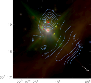
Figure 1: Integrated intensity map of [C ii] overlaid on a Spitzer IRAC false-color image of the same region. The IRAC map uses the logarithmic intensities of the 3.6, 5.6 and 8$\,\mathrm{\mu m}$ channels. The integrated intensity contours are drawn at 50, 70, 90, 120, 150, 180 K $\,\mathrm{km\,s^{-1}}$. The external cloud interface is visible in the south-west. The arrow shows the direction towards the illuminating source HD 211880. The red marks indicate the position of the known infrared sources: south-west is IRS 1, the northern one is IRS 2, and the south-east we find IRS 3 (Evans et al., 1989), the yellow marks show position of known submm cores (Minchin et al., 1995; Maud et al., 2013). The IRAC peak falls at the location of IRS 1.

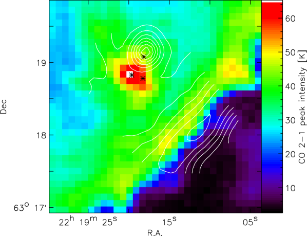
Figure 2: Peak intensity map of [C ii] overlaid on a IRAM 30m map of the CO 2–1 peak intensity. The [C ii] contours are drawn at 15, 20, 25, 30, 35, 40, 45 K. The black marks indicate the positions of IRS 1-3.

Figure 1 shows the observed integrated intensity map of the [C ii] line superimposed on a Spitzer IRAC image of the cloud composed of the 3.6, 5.6 and 8$\,\mathrm{\mu m}$ channels. The IRAC image emphasizes two structures in the cloud. The peak in all bands is given by the embedded source IRS 1, relatively deep in the cloud. The embedded cluster produces about $10^{4}$ solar luminosities, $L_{\odot}$, heating the dust to temperatures of up to 1400 K (Koumpia et al., 2015). In the south-west we see the cloud surface illuminated by HD 211880 as a red band-like structure due to the excitation of PAHs at this external PDR. On top of these dominant features, we see some smaller spots east of IRS 1 close to IRS 3, bright in 5.6 $\,\mathrm{\mu m}$ emission. The [C ii] emission traces the front of the PDR in the south-west through a secondary peak, but has a clear maximum 20^′′ north of IRS 1, slightly north of IRS 2.

To compare the fine structure lines with the molecular cloud material we use the maps of CO 1–0, 2–1, C¹⁸O 1–0, and ¹³CO 1–0 taken with the IRAM 30m telescope, presented and discussed by Koumpia et al. (2015). Figure 2 compares the [C ii] peak intensities with the CO 2–1 peak intensity map. The spatial distribution of the CO 2–1 line shows a behavior similar to the mid-infrared continuum. CO 2–1 peaks about 20^′′ south of the [C ii] peak in a region covering IRS 1 and IRS 3. The CO 2–1 maximum falls close to IRS 3 and at the cloud surface the line is brighter than deep in the cloud. There is a clear layering with [C ii] peaking closer to the illuminating star and CO 2–1 deeper in the molecular cloud, as expected from standard PDR models (see e.g. Hollenbach & Tielens, 1999). The location of the peak of [C ii] emission at the cloud surface therefore represents an expected morphology, but the relative shift of the emission peak to the north of IRS 1 is a striking unexpected feature in the [C ii] maps.

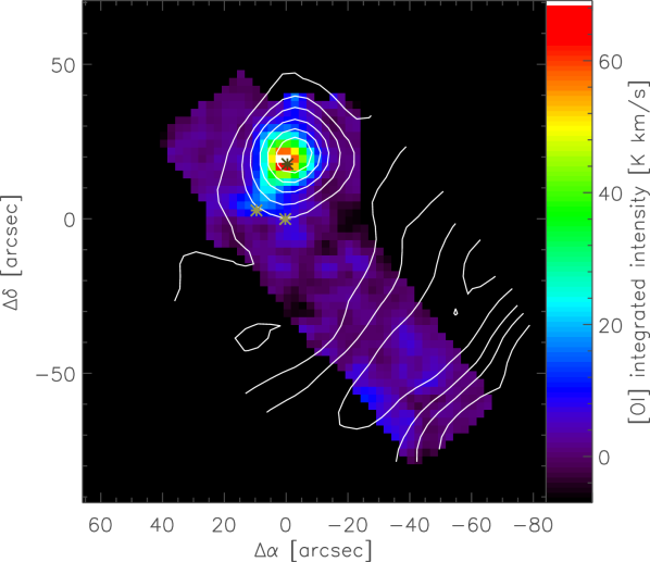
Figure 3: Integrated intensity map of the [O i] 63 $\,\mathrm{\mu m}$ line (colors) overlaid by contours of the [C ii] integrated intensity (levels as in Fig. 1). The black marks indicate the positions of IRS 1-3. All coordinates are taken relative to the position of IRS 1 at R.A.$=22^{\rm h}{}19^{\rm m}{}18^{\rm s}{}.21$, Dec$=63^{\circ}{}18^{\prime}46^{\prime\prime}.9$ (J2000)

Figure 3 compares the [C ii] with the [O i] 63 $\,\mathrm{\mu m}$ line integrated intensity. The [O i] map shows a good match of the emission peak with that of [C ii]. The peak is strongly concentrated and dominates the overall map. [O i] also peaks slightly north of IRS 2; it may be offset from the center of the [C ii] peak by about 2^′′, but this is close to our pointing accuracy. The location of the [C ii] and [O i] peak indicates an association with IRS 2, similar to an already known small continuum feature visible at mid-infrared wavelengths (Harvey et al., 2012). The [O i] peak is slightly elongated towards the south-east in the direction towards IRS 3. IRS 1 is not prominent at all in [O i]. We also see a slightly increased [O i] intensity at the cloud interface in the region where [C ii] peaks. Unfortunately, the data quality does not allow to discriminate whether there is any relative offset between the two fine structure line peaks in that region.

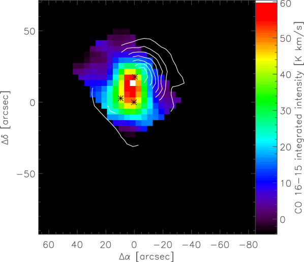
Figure 4: Integrated intensity map of CO 16–15 with contours of CO 13–12 drawn at levels of 10, 20, 30, 40, 50, 60, 70 K $\,\mathrm{km\,s^{-1}}$. Only the region around IRS 1 has been observed in CO 16–15; in CO 13–12 only two outer strips have been covered avoiding the center. The black marks indicate the positions of IRS 1-3.

Figure 4 shows the integrated intensities of the CO 13–12 and 16–15 lines. Unfortunately, only complementary regions were mapped in the two lines with narrow overlapping strips. Therefore, the CO 13–12 observations are hardly useful to understand the nature of the peak seen in the fine-structure lines. We see, however, that both high-$J$ CO lines show a more extended emission around the central sources compared to the fine-structure lines. The CO 16–15 peak falls between IRS 1 and IRS 2, i.e. we see a superposition of hot CO emission from both IRS 1 and from the fine-structure line peak close to IRS 2. The high-$J$ CO lines trace both components in a similar way; they show an intermediate behavior between the fine-structure lines and the low-$J$ CO.

3.1 Line profiles

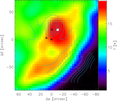
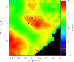
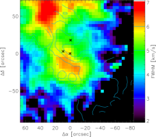
Figure 5: Peak intensity, first moment (centroid velocity) and second moment (translated to FWHM) of the lines of ¹³CO 1–0 (colors) and [C ii] contours. The black marks indicate the positions of IRS 1-3. The contour levels for the [C ii] peak intensity match those from Fig. 2, for the line position they are given at -9.5, -8.5, -7.5, -6.5 $\,\mathrm{km\,s^{-1}}$, and for the line width at 3, 4, 5, 6 $\,\mathrm{km\,s^{-1}}$. Velocities are given in LSR and intensities in main beam temperatures.

In all the published maps of S 140 only the ¹³CO 1–0 line peak intensity also has a global maximum close to IRS 2. To understand the nature of the fine-structure line peak it is, therefore, worth to compare our observations with the ¹³CO 1–0 data more carefully, including the velocity structure. ¹³CO 1–0 is optically thin over most parts of the map. Koumpia et al. (2015) measured optical depths of about 0.3 for most of the gas and a maximum value of 0.8 that is still marginally optically thin. Figure 5 compares the distribution of the peak intensity, the mean line velocity, and the line width of the ¹³CO 1–0 line with the corresponding parameters from the [C ii] line.

The relative proximity of the ¹³CO 1–0 peak and the [C ii] and [O i] peaks seem to be accidental as the overall morphology of the line maps shows no other similarities. The ¹³CO 1–0 emission is much more extended and has about the same level at the positions of IRS 2 and IRS 1. When inspecting the ¹³CO 1–0 integrated intensity, we find the same behavior as seen in the other molecular line tracers with a maximum close to IRS 1. A second similarity in the peak intensities of ¹³CO 1–0 and [C ii] are the relatively low values south of IRS 1. The spot matches the southern part of the molecular outflow discussed e.g. by Maud et al. (2013). The outflow is driven from IRS 1 pointing towards the north-west and south-east, leading to the velocity gradient seen e.g. in the ¹³CO 1–0 line position map around IRS 1. At the location of the southern outflow [C ii] is hardly present at all, but the ¹³CO 1–0 line is prominent, tracing the outflow through broad line wings (see Fig. 5c) that lead to a large integrated intensity there in spite of the lower peak intensity.

The [C ii] line shows the largest line width north-west of IRS 1, in the direction of the northern outflow, but only a moderate line width at the location of the intensity peak close to IRS 2. We find a trend of anti-correlation between the [C ii] lines and the ¹³CO 1–0 lines. The ¹³CO 1–0 lines are broad in a ridge south-east and north-east of the cluster that is associated with low center velocities while [C ii] shows the broadest lines west of the cluster. Except for the southern outflow region and the north-eastern boundary of the map, the [C ii] profiles are always somewhat broader than the ¹³CO 1–0 profiles. We interpret this as being due to optical depth broadening (see below).

When inspecting the line positions, the ¹³CO 1–0 profiles are dominated by the outflow pattern with slightly blue shifted velocities south-east of IRS 1 and red shifted velocities in the opposite direction. Overall, the variations are relatively small. In contrast, [C ii] shows a clear offset in the line velocity for the bright emission component close to IRS 2. While in most of the map the [C ii] line has the same velocity of about $-8$ $\,\mathrm{km\,s^{-1}}$ as the bulk of the ¹³CO gas, the peak source has a significantly lower velocity of about $-6.5$ $\,\mathrm{km\,s^{-1}}$. This indicates that the bright emission source is only weakly associated with the rest of the gas and not seen in ¹³CO.

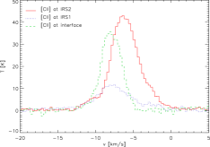
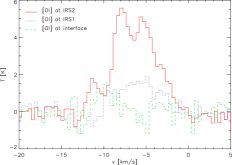
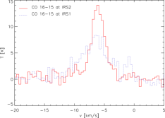
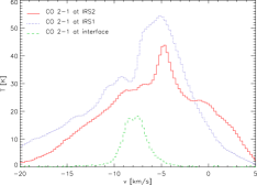
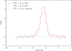
Figure 6: Line profiles of the [C ii], [O i], CO 16–15, CO 2–1, C¹⁸O 1–0, and ¹³CO 1–0 lines at the position of the [O i] peak (0,20 close to IRS 2), at IRS 1 (0,0), and at the interface (-40,-54). The lines are averaged in a Gaussian beam of 17.3^′′ FWHM (telescope + convolution kernel) except for the ¹³CO and C¹⁸O lines that can be only treated at the lower resolution of 23^′′.

Figure 6 shows the line profiles of [C ii], [O i], CO 16–15, CO 2–1, C¹⁸O 1–0 and ¹³CO 1–0 at the location of the fine-structure line peak close to IRS 2, at the position of the main heating source IRS 1, and at the external cloud interface. All lines trace the interface at a velocity of about $-8$ $\,\mathrm{km\,s^{-1}}$. The [O i] line is only marginally detected there, [C ii] and the CO lines are narrow with a width of 3–4 $\,\mathrm{km\,s^{-1}}$. The velocity of this PDR surface is slightly different from the large scale velocity field of the thin surrounding medium measured through the broad H i line in the $36^{\prime}$ beam of the Leiden/Dwingeloo survey to peak at -7 $\,\mathrm{km\,s^{-1}}$ (Kalberla et al., 2005).

Towards IRS 2, [C ii] peaks at -6.5 $\,\mathrm{km\,s^{-1}}$, offset in velocity from the bulk of the gas, as seen already in Fig. 5. The [O i] line shows a dip at this velocity and two peaks at the velocities of $-5.5$ $\,\mathrm{km\,s^{-1}}$ and $-8$ $\,\mathrm{km\,s^{-1}}$ coinciding with the peak velocities seen in CO 2–1 towards IRS 2 and towards the interface. However, as there is only weak [O i] emission from the interface, we think that this coincidence is accidental and we rather see in [O i] the same material that we trace in [C ii], indicating that [O i] exhibits a self-absorption dip where [C ii] peaks instead of two velocity components.

CO 2–1 traces mainly other gas. We find broad outflow wings from the molecular outflow (Maud et al., 2013), only seen in the low-$J$ CO lines. The optically thin lines of CO 16–15 and ¹³CO 1–0 are narrow at the peak suggesting that even the [C ii] line is broadened by a significant optical depth. The comparison of the fine structure lines and CO 16–15 at IRS 1 shows that [C ii] only traces the velocity component matching the interface velocity there, but no emission at $-6$ $\,\mathrm{km\,s^{-1}}$, while CO 16-15 and [O i] show a stronger emission in the $-6$ $\,\mathrm{km\,s^{-1}}$ component and a weaker emission with the interface velocity there. This means that we find several gas components with different velocities and chemical properties towards IRS 1.

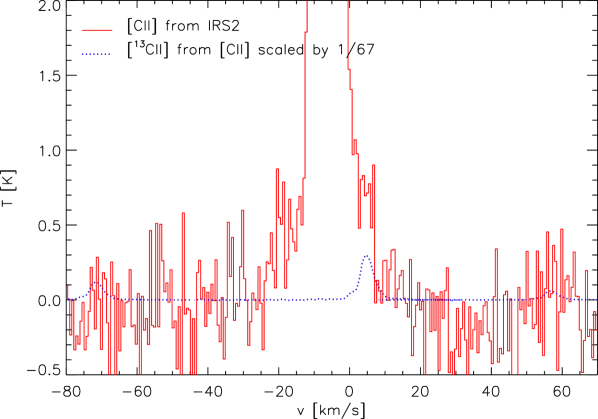
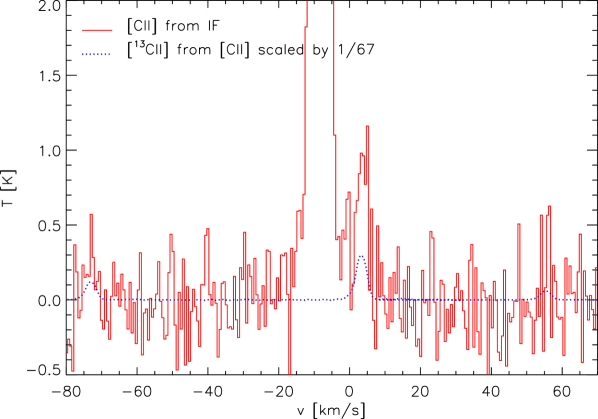
Figure 7: Baseline of the [C ii] profiles showing the hyperfine components of the [¹³C ii] transitions. The upper plots shows the sum spectrum from all spectra with integrated intensities above 100 K $\,\mathrm{km\,s^{-1}}$ from the IRS 1-3 region, the lower plot from the interface region. The blue lines represent the same spectra scaled by an abundance ratio of 1/67 and the corresponding line ratio and frequency of the three hyperfine transitions, i.e. they represent the spectrum that we expect in case of an optically thin [C ii] line.

To estimate the optical depth of the [C ii] line, based on the line profiles, we can use two approaches: derive the optical-depth line broadening by comparing the line width with an optically thin tracer, and to compare the line intensity with an optically thin tracer not affected by abundance or excitation uncertainties, namely the [¹³C ii] transitions. In the first approach, we assume a Gaussian velocity dispersion and obtain the optical depth at the line peak from the measured line broadening $\sigma_{\rm line}\approx(1+0.115\hat{\tau})\;\sigma_{\rm vel}$ where $\hat{\tau}$ is the line-center optical depth (Phillips et al., 1979; Ossenkopf et al., 2013). Using the optically thin ¹³CO 1-0 to measure the true velocity dispersion, we can translate Fig. 5c into a [C ii] optical depth map, except for the region south of IRS 1 where the ¹³CO 1–0 line is broader than [C ii] due to the molecular outflow. For the interface, we obtain a ¹³CO 1–0 line width of 3 $\,\mathrm{km\,s^{-1}}$ and a [C ii] line width of 4 $\,\mathrm{km\,s^{-1}}$, in the region between IRS 1 and IRS 2, the line widths are 5 and 6 $\,\mathrm{km\,s^{-1}}$, respectively. This translates into [C ii] peak optical depths of three towards the interface and two towards the central cluster.

Figure 7 shows the corresponding [¹³C ii] spectra measured in the two regions. They are compared with a scaled version of the [C ii] line, reduced in intensity by the typical ¹³C/¹²C abundance ratio of 1/67 in the solar neighborhood (Langer & Penzias, 1990, 1993) and the relative weights of the hyperfine components (0.625 at 11 $\,\mathrm{km\,s^{-1}}$, 0.25 at -65 $\,\mathrm{km\,s^{-1}}$, 0.125 at 63 $\,\mathrm{km\,s^{-1}}$ relative to [C ii], Ossenkopf et al., 2013). Towards the interface the two stronger hyperfine components are clearly detected. The peak intensity of the [¹³C ii] is 3.1 times as high as expected from the [C ii] line when assuming optically thin [C ii] emission. This can be translated into a line-center optical depth of about three. Towards the embedded cluster, the strongest component appears as a shoulder of the broader [C ii] line and the two weaker components are barely visible. The factor 2.2 difference between observed intensity and scaled optically thin [C ii] emission is also in agreement with a line-center optical depth of two as measured from the line broadening. Both approaches, therefore provide matching results for the [C ii] optical depth towards the two peaks of [C ii] emission.

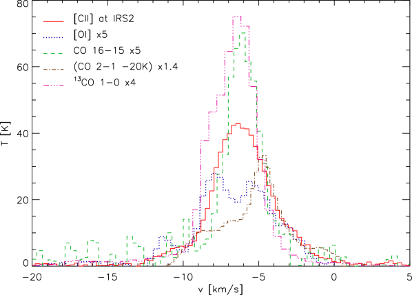
Figure 8: Line profiles of the [C ii], [O i], CO 2–1, CO 16–15, and ¹³CO 1–0 lines at the position of the [O i] peak (0,20). The lines were scaled to similar intensities at -4 $\,\mathrm{km\,s^{-1}}$. For CO 2-1, a constant emission of 20 K is subtracted to exclude the extended outflow emission.

To resolve the intrinsic velocity profile of the main emission source at IRS 2 we compare scaled versions of the different profiles towards this source in Fig. 8. The scaling factors in the plot were adjusted to allow for a comparison of the red wing of the profiles at sufficiently high velocities to not be affected by self-absorption or saturation from high optical depths. For CO 2-1 we also had to subtract the very extended outflow contribution (see Fig. 6). The C¹⁸O 1–0 line is not shown here as it matches almost exactly the shape of the CO 16–15 line. A comparison of the blue wing of the profiles provides no information on the source at IRS 2 as this velocity interval is heavily affected by emission and (self-) absorption from the bulk of the gas in S 140 at -8 $\,\mathrm{km\,s^{-1}}$.

We find an almost perfect match of the red wing shape of the three (partially) optically thick lines of [C ii], [O i], and CO 2–1. In contrast, the thin lines of ¹³CO 1–0 and CO 16–15 are clearly narrower, not allowing to fit the same wing. Optical depth broadening of the lines must play a significant role. The peak of the CO 16–15 line coincides with the absorption dip seen in [O i] and CO 2–1. The narrow shape of the peak of the CO 2–1 line at -4.7 $\,\mathrm{km\,s^{-1}}$ results from this absorption out of a broader emission component. The shoulder seen in the ¹³CO 1-0 and CO 2–1 lines at -8 $\,\mathrm{km\,s^{-1}}$ probably traces emission from IRS 1 or the extended molecular cloud material. Overall, the lines are consistent with the velocity dispersion as measured by the CO 16–15 and C¹⁸O 1–0 lines of only 2.4 $\,\mathrm{km\,s^{-1}}$ (FWHM), but an optical-depth broadening of the fine-structure lines.

For the optically thick lines, the intrinsic line intensity from the emission peak therefore should be higher than our observed integrated intensity. For [C ii], the profiles are consistent with the optical depth of about two, leading to a 45 % reduction of the integrated line intensity compared to optically thin emission. For [O i], we see, however, a clear self-absorption signature due to gas in the foreground with lower excitation temperature. That makes an estimate of the intrinsic intensity from the emission peak difficult. If we assume that the red wing is not affected by self absorption, we can use the ratio of the integrated line intensity between [C ii] and [O i] seen in Fig. 8 as an estimate for the missing flux in the [O i] line. This indicates that the source intrinsic line flux should be higher by about 50 % without foreground absorption.

From the information given in the line profiles we can already conclude that the [O i] and [C ii] emission does not seem to be related to the known outflow activity in S 140, probably rather tracing PDR interfaces. While [C ii] and [O i] are both bright at IRS 2, only [C ii] is bright at the cloud surface and [O i] is barely detected there. As the [O i] line has a critical density of $5\times 10^{5}$ cm^-3 (Jaquet et al., 1992, see Tab.LABEL:tab_greatlines), 100 times the critical density of the [C ii] line, this probably reflects the lower density of the interface region. In contrast, at the fine structure line peak position, the gas must be dense and optically thick for [O i] so that the same material produces an almost Gaussian line in [C ii] and a double-peak-shaped line in [O i]. The optically very thick CO 2–1 line only reveals a prominent red shifted wing towards IRS 2. This would be consistent with an expansion scenario of the source.

4 Properties of the gas

4.1 Gas parameters across the GREAT map

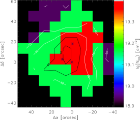
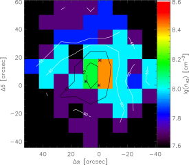
Figure 9: CO column density (upper plot: colors), gas density (lower plot: colors), and kinetic temperature (both plots: contours) derived from the RADEX fit of the integrated intensities of the observed lines of CO 1–0, 2–1, 16–15 and the isotopologues ¹³CO 1–0 and C¹⁸O 1–0.

As a first step to understand the nature of the fine structure lines we need to know the properties of the gas across the map. This can be done by analyzing the molecular lines of CO and its isotopologues based on our high-$J$ CO observations and the complementary low-$J$ CO, ¹³CO, and C¹⁸O IRAM data from Koumpia et al. (2015). When knowing the column density, the volume density and kinetic temperature of the gas we can compute column density maps of [C ii] and [O i] from the measured fine-structure line intensities.

We performed a fit of the CO (and isotopologues) line intensities using the non–LTE radiative transfer code RADEX (van der Tak et al., 2007) that computes the line intensities of a molecule for a set of physical parameters: kinetic temperature, H₂ gas density, molecular column density, background temperature and line width. We used the maps of CO 1–0, 2–1, ¹³CO 1–0, C¹⁸O 1–0, and CO 16–15 to perform a $\chi^{2}$ minimization fit for a range of kinetic temperatures (30–700 K), column densities (10¹⁷ – 4$\times$ 10¹⁹ cm^-2) and volume H₂ densities (10⁵ – 5$\times$ 10¹⁰ cm^-3). In the area covered by the CO 16–15 map we have enough observational constraints to determine those 3 free fitting parameters. For all calculations we used a fixed line width value of 3.5 km s^-1. We adopted a cosmic background radiation field of 2.73 K and used the molecular data from the LAMDA database (Schöier et al., 2005).

Figure 9 shows the resulting distributions of the gas temperature, density, and column density of CO. As the CO 16–15 line has an upper level energy of 750 K and a critical density of $10^{6}$ $\,\mathrm{cm^{-3}}$ (see Table LABEL:tab_greatlines), one would expect that the strong line drives the solution to high temperatures and densities in the order of the critical density. However, it turns out that the low-$J$ lines can only be fitted with lower temperatures. To excite the CO 16-15 line, RADEX then has to increase the gas density to values in the order of $10^{8}$ $\,\mathrm{cm^{-3}}$, a value much higher than derived in all other ways. This is a strong indication that the assumption of uniform gas parameters within the individual pixels of our map is not justified in S 140. It is much more likely that the true gas composition consists of a cooler component, mainly traced by the low-$J$ CO (and isotopologues) lines, while a second hot component is responsible for the CO 16–15 line.

As all other lines discussed here are insensitive to gas densities above $10^{6}$$\,\mathrm{cm^{-3}}$, the overestimate of the gas density obtained in this way should be irrelevant for the further analysis. The RADEX fit shows that the gas temperature peaks between IRS 1 and IRS 2, roughly matching the CO 16–15 intensity map. The density structure shows a density peak at the positions of IRS 1 and IRS 2. The column density follows mainly the distribution of the isotopologues which is higher towards the west region of the sources. It matches roughly the column density structure that was determined from FORCAST, PACS, and SCUBA dust observations in Koumpia et al. (2015). They also found a column density peak about 20^′′ west of IRS 1 and IRS 2 and a smaller peak somewhat east of IRS 2.

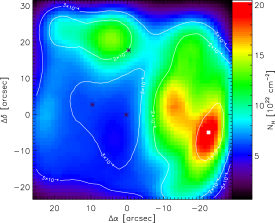
Figure 10: Column density map of gas derived from FORCAST, PACS, and SCUBA continuum observations in the center of the region (colors), overlaid by contours of the CO abundance, running from $1\times 10^{-4}$ to $3\times 10^{-4}$.

The CO column densities can be translated into abundances if we know the gas column from the dust observations of the central region. To derive gas column densities from the 100$\,\mathrm{\mu m}$ dust opacity map, we use the dust properties of model 5 from Ossenkopf & Henning (1994) following the discussion in Koumpia et al. (2015) and the standard conversion factor of $N_{\rm H}/A_{V}=1.9\times 10^{21}$ cm^-2 (Bohlin et al., 1978). This provides a 100 $\,\mathrm{\mu m}$ optical depth of $1.30\times 10^{-24}$ cm${}^{2}\times(N_{\rm H}+2N_{\rm H_{2}})$. The resulting column density map is shown in Fig. 10.

The contours in the figure give the CO abundance computed by dividing the CO column from Fig.9 by the dust-based gas column density. For most of the cloud we find values of $X($CO$)=N_{\rm CO}/(N_{\rm H}+2N_{\rm H_{2}})$ around $2-3\times 10^{-4}$. Lower values of about $1\times 10^{-4}$ are found at the submm-peak west of IRS 1. Somewhat lower values are also found towards IRS 2 and somewhat higher values occur at the positions of IRS 1 and IRS 3. A reduction of the CO abundance towards IRS 2 would be consistent with the conversion of molecular material to atomic and ionized material seen in the bright fine-structure lines. The stronger decrease towards the submm peak could indicate CO freeze-out in very cold and dense material. But overall, the abundance variations within the map are about as large as the uncertainty from the dust column.

A CO abundance of more than $2\times 10^{-4}$ would actually exceed the total amount of carbon available in the gas phase (see e.g. Cardelli et al., 1993). Blake et al. (1987) measured values $X($CO$)$ of only $6\times 10^{-5}$ towards the dense molecular material in the Orion molecular cloud and $2.5-3\times 10^{-5}$ in several clouds on larger scales, probably involving more atomic and ionized carbon. A higher CO abundance of $1.3\times 10^{-4}$ has been measured towards NGC 2024 by Lacy et al. (1994). Our systematically higher abundances can be explained by the uncertainty of the dust properties covering a factor 2–3 in the 100 $\,\mathrm{\mu m}$ opacity (Ossenkopf & Henning, 1994). When assuming a dust model with a two times lower 100 $\,\mathrm{\mu m}$ opacity, the columns in Fig. 10 increase by a factor two, the abundance values decrease by the same factor, and we obtain values close to those from Lacy et al. (1994). Unfortunately, the resolution of the low-$J$ CO maps is insufficient to determine the gas column density with the same resolution as the dust opacity. Hence, we can only conclude that the CO column densities are close to the upper edge of the range expected from the dust column densities. This means that most of the gas must be molecular so that we can use CO as a proxy for the total gas column in S140. This is consistent with the strong spatial confinement of the fine-structure line emission in S140 indicating that CO provides a reasonable measure for the total gas column density, even if not all gas is molecular. Assuming $X($CO$)=1.3\times 10^{-4}$ we obtain hydrogen column densities $N_{\rm H}=N_{\rm H}+2N_{\rm H_{2}}$ between $7\times 10^{22}$ cm^-2 and $1.97\times 10^{23}$ cm^-2 within the map covered by the CO 16-15 observations.

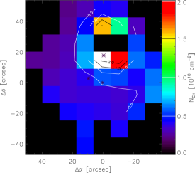
Figure 11: Column density map of C⁺ derived from the measured [C ii] intensities using the gas parameters from the RADEX fit to the CO lines. The contours show the [C ii] line optical depth a levels of $\tau=0.5,1.0,1.5,2.0$. In the two pixels north of IRS 2, the optical depth is too large for a reliable column density estimate.

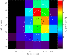
Figure 12: Column density map of atomic oxygen derived from the measured [O i] intensities using the gas parameters from the RADEX fit to the CO lines. The contours show the [O i] line optical depth at levels of $\tau=0.05,0.10,0.15,0.20$.

In the next step we can use the kinetic temperature and volume density from the RADEX fit of the CO lines (Fig. 9) to compute the C⁺ and atomic oxygen column densities from the [C ii] and [O i] observations. This allows to compare the abundance of the different species in the gas within the telescope beam along the line of sight. Actually, we do not expect that all species are spatially co-existing – we rather expect abundance gradients along the path and within the area of the beam – but the volume-integrated abundances can be easily compared with the results from more complex models and other Galactic and extragalactic observations. The CO 16–15 line provides strong constraints on the parameters derived from the RADEX fit and it is mainly stemming from hot and dense gas, the same gas that should also provide the main contribution to the fine-structure line emission. Therefore, the error made in assuming the same excitation conditions as seen by CO for deriving the C⁺ and oxygen column densities should be smaller than the factor two uncertainty that we have to face for the gas column anyway. To be consistent with the RADEX fit, we restrict the integration to the same velocity interval from -8.4 to -4.4 km s^-1. Fig. 11 and Fig. 12 show the resulting column densities and the optical depths of the lines. Although the line profiles of [O i] indicate optically thick line (Fig. 6), our resulting optical depths are $\tau<1$. This is probably due to the strong self-absorption in the line creating an intensity dip for the considered velocity range, leading to too low column densities and optical depths. The [C ii] analysis results in column densities 2.2$\times$10¹⁷ – 2$\times$10¹⁸ cm^-3 and a range of optical depths 0.28–2.31 with the higher values to be closer to IRS 2 in agreement with the estimate from the line profile in Sect. 3.1.

With the hydrogen column densities from CO the C⁺ column density map translates into C⁺/H abundances, $X($C${}^{+})$, between $1.1\times 10^{-5}$ around the fine-structure line peak and $2-3\times 10^{-6}$ for the rest of the map. For the oxygen abundance, we find values between $4\times 10^{-5}$ around IRS 2 and $1.0-1.5\times 10^{-5}$ for the rest of the map. For both species the abundance at IRS 1 is as low as in the rest of the map outside of the fine-structure line emission peak.

These values can be compared to PDR models (Röllig et al., 2007). At a PDR surface, almost all carbon is in the form of C⁺. For diffuse clouds, Sofia et al. (2004) measured a C⁺ abundance of $X($C${}^{+})=1.6\times 10^{-4}$, but in dense regions a larger fraction of carbon is incorporated in dust and PAHs leading to a PDR surface abundance of $X($C${}^{+})=1.2\times 10^{-4}$ in dense clouds (Wakelam & Herbst, 2008). Deeper in the clouds where the UV is sufficiently shielded, C⁺ turns into atomic carbon and subsequently into CO, so that the C⁺ abundance falls by three to four orders of magnitude, depending on the cosmic ray ionization rate. Even our value for IRS 2 falls much below the PDR surface limit, confirming that only in a small gas fraction carbon is ionized through UV radiation while most of the gas is molecular. The column of molecular material should be at least ten times deeper than the C⁺ column produced in a PDR around IRS 2.

Depending on the local conditions the oxygen abundance in dense clouds should not vary by more than a factor three. In the high-UV field limit, almost all gas-phase oxygen is in atomic oxygen, resulting in an abundance of $X($O$)=3\times 10^{-4}$ relative to hydrogen. Deep in molecular clouds, most oxygen is incorporated in CO so that only $X($O$)=1\times 10^{-4}$ is left in the gas phase. Our measured abundance still falls below this lower limit. This can be explained by the fact that most oxygen is probably at temperatures below the range of 50–70 K fitted by RADEX for a homogeneous gas. The colder oxygen does not contribute to the fitted emission, but rather creates the absorption seen in our [O i] line profiles.

4.2 The [C ii] and [O i] peak

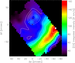
Figure 13: Intensity map of [O i] (top), [C ii] (center), and CO 16–15 (bottom) after subtracting a Gaussian intensity distribution of FWHM$=8.3^{\prime\prime}$ from the observed map. The overlaid contours show the original intensity maps at levels of 8, 24, 40, 56, 72 K $\,\mathrm{km\,s^{-1}}$ ([O i]), 50,70,90,120,150,180 K $\,\mathrm{km\,s^{-1}}$ (CII), and 10, 20, 30, 40, 50, 60 K (CO 16–15).

To estimate the size of the region responsible for the fine-structure line emission peak, we fitted the observed [O i] integrated intensity map by a Gaussian intensity distribution peaking close to IRS 2 convolved with the telescope beam at 4.7 THz. The [O i] map provides the main constraint to the source size due to the smaller beam compared to [C ii] and the CO lines. We allowed for a 2 arcsec pointing jitter in the fit when adjusting the location of the peak. The best fit leading to a relatively smooth background after the source subtraction is obtained for a source FWHM of 8.3^′′ and a peak intensity of 76 K $\,\mathrm{km\,s^{-1}}$. Figure 13 (top panel) shows the result. We see that the subtracted source covered 80 % of the intensity at the position of the peak, but that there remains a somewhat more extended emission structure north of IRS 1. IRS 1 is part of that structure, but shows no concentrated [O i] emission associated with the infrared source. In contrast, we find a secondary [O i] peak slightly north of IRS 3, the weakest infrared source in the field.

A priori, the spatial extent of the emission in [O i] and [C ii] can be different, but if we subtract a source with the same size and the peak intensity of 212 K $\,\mathrm{km\,s^{-1}}$ from the [C ii] map we also obtain a very smooth map with no further indications of the IRS 2 contribution (Figure 13, central panel). This suggests that we see about the same gas responsible for the peak in [O i] and [C ii] spatially well confined to a region close to IRS 2. Repeating the same experiment for the CO 16–15 map, provides a peak intensity of 46 K $\,\mathrm{km\,s^{-1}}$, but a clear residual of emission from IRS 1 and IRS 3 (Figure 13, bottom panel). This agrees with the previous analysis of Koumpia et al. (2015) finding extended hot molecular gas around IRS 1.

The identification of a spatially well confined emission structure close to IRS 2, responsible for the observed strong fine-structure line emission allows to quantify the properties of the emitting gas. With an FWHM of 8.3^′′ we obtain a spatial angle of the emitting region of $1.8\times 10^{-9}$ sr and a diameter of 0.03 pc. This allows to compute absolute luminosities from the integrated intensities and the source projected area of $1.0\times 10^{34}$ cm² assuming isotropic radiation. For the [O i] line we obtain 0.28 $L_{\rm\odot}$ and for the [C ii] line 0.05 $L_{\rm\odot}$. This can be compared to the total energy input at that location. Koumpia et al. (2015) estimated a total luminosity of the source at IRS 2 of 2000 $L_{\rm\odot}$. This means that only 0.016 % of the source luminosity is radiated away in the two fine-structure cooling lines. We will further discuss this in Sect. 4.4.

For the CO 16–15 line we obtain a corresponding luminosity of only 0.01 $L_{\rm\odot}$, but over the full CO ladder this will add up to a considerable net cooling. If we make the extremely conservative assumption that all CO line intensities are constant at the value of the 16–15 transition for lower $J$ transitions and zero for higher transitions, we obtain a lower limit for the CO cooling luminosity of 0.045 $L_{\rm\odot}$ already matching the [C ii] luminosity. If we use the full SED ladder fit to the narrowest line component from the next section (4.3), we obtain instead a cooling power of 0.096 $L_{\rm\odot}$ and if we include the emission over the total line width, the CO luminosity sums up to 0.13 $L_{\rm\odot}$, i.e. a value that is about half the cooling power in the [O i] line. In spite of the prominent fine-structure line peak at IRS 2, we thus find a situation where the molecular line cooling is relatively important next to the fine structure line cooling. This is similar to the situation found in other protostars (Karska et al., 2013). Obviously, the situation is even more extreme for IRS1, where we measure strong high-$J$ CO emission, but basically no [C ii].

We can estimate the gas column density from the integrated [C ii] line intensity, by using the relatively constant [C ii] emissivity per column density (Eq. (2) from Ossenkopf et al., 2013). For a temperature of about 200 K we obtain:

$$\int\!\!\epsilon\,dv\approx 560\;\frac{\rm K\,kms^{-1}}{\rm cm^{-3}\leavevmode\nobreak\ pc}\times N_{{\rm C}^{+}}$$ (1)

As the emissivity is only weakly temperature-dependent, this value applies within a 15 % error bar to all excitation temperatures between 100 K and 500 K, covering the typical range expected in PDRs. Eq. (1) provides a direct translation of intensity to column density for optically thin emission. Because we know the optical depth from Sect. 3.1 the equation can also be used with the corresponding optical depth correction of 45 % to compute the C⁺ column density for IRS 2.

We obtain a C⁺ column density of $1.7\times 10^{18}$ cm^-2. This is slightly lower than the value of $2\times 10^{18}$ cm^-2 obtained for the total [C ii] emission towards IRS 2 measured in the RADEX simulation for the full map in Sect. 4.1. However, here we consider only the 73 % of the [C ii] emission at that position that are attributed to the compact source ignoring a small part of the total column density. Using the carbon gas-phase abundance of $1.2\times 10^{-4}$ for dense clouds (Wakelam & Herbst, 2008) (see Sect.4.1) and assuming that all carbon is ionized, the C⁺ column density of $1.7\times 10^{18}$ cm^-2 provides a lower limit for the total column density of the [C ii] emitting gas of $1.4\times 10^{22}$ cm^-2. Higher values result for partial ionization. If we assume that the [C ii]-emitting gas fills the observed emitting volume of $1.0\times 10^{51}$ $\,\mathrm{cm^{3}}$, we deduce a minimum gas density of $1.4\times 10^{5}$ $\,\mathrm{cm^{-3}}$. The derived optical depth of the clump seen in dust emission close to IRS 2 is, however, $A_{\rm V}\approx 100$ (Koumpia et al., 2015) corresponding to gas column densities of $2\times 10^{23}$ $\,\mathrm{cm^{-2}}$. That means, that only 7 % of the gas is emitting in [C ii]. This could be explained by clumpiness of the gas within the 8.3^′′ peak and high-density clumps, or more naturally, by a PDR layering structure where the [C ii] emission only stems from gas with $A_{\rm V}\la 2$ facing the embedded sources.

Unfortunately, it is not possible to perform the same estimate for the [O i] emission. The high-temperature LTE limit of the [O i] emissivity is about three times as large as for [C ii] (Eq. 1), but it only applies to densities above $10^{6}$ $\,\mathrm{cm^{-3}}$ and temperatures above 200 K, and it also requires optically thin emission or an accurate estimate. The line profiles showed already that [O i] is optically very thick and the intensity of the [O i] line is three times lower than that of [C ii]. To check the consistency of the parameters in the frame of a real radiative transfer computation we perform RADEX runs in the next section.

4.3 RADEX fit of individual sources

Table 2: Line parameters of the narrow component of CO and isotopologues towards IRS 1 and IRS 2 – GREAT, IRAM & HIFI data.

		IRS 1			IRS 2			interface
Line	$v_{\rm LSR}$	FWHM	$\int$ T${}_{mb}dv$	$v_{\rm LSR}$	FWHM	$\int$ T${}_{mb}dv$	$v_{\rm LSR}$	FWHM	$\int$ T${}_{mb}dv$
	[km s-1]	[km s-1]	[K $\,\mathrm{km\,s^{-1}}$]	[km s-1]	[km s-1]	[K $\,\mathrm{km\,s^{-1}}$]	[km s-1]	[km s-1]	[K $\,\mathrm{km\,s^{-1}}$]
CO 9–8	$-5.78\pm 0.01$	$4.87\pm 0.06$	$117\pm 2$	…	…	…	$-7.80\pm 0.07$	$2.50\pm 0.20$	$1.20\pm 0.20$
CO 13–12	…	…	…	$-6.76\pm 0.03$	$3.30\pm 0.08$	$71.1\pm 1.4$	…	…	…
CO 16–15	$-6.55\pm 0.06$	$3.5\pm 0.2$	$40.3\pm 1.7$	$-6.43\pm 0.04$	$2.7\pm 0.1$	$37.2\pm 1.3$	…	…	…
13CO 1–0	$-6.45\pm 0.03$	$2.48\pm 0.09$	$28.7\pm 1.9$	$-6.54\pm 0.06$	$2.6\pm 0.1$	$49.4\pm 1.8$	$-8.12\pm 0.37$	$1.34\pm 0.70$	$0.84\pm 0.26$
13CO 10–9	$-6.71\pm 0.02$	$2.41\pm 0.08$	$12.8\pm 1.1$	…	…	…	…	…	$<3\sigma$
C18O 1–0	$-6.52\pm 0.05$	$2.4\pm 0.1$	$6.8\pm 0.6$	$-6.64\pm 0.04$	$2.36\pm 0.1$	$8.4\pm 0.1$	…	…	$<3\sigma$
C18O 9–8	$-6.7\pm 0.1$	$2.6\pm 0.2$	$2.8\pm 0.3$	…	…	…	…	…	$<3\sigma$
[C ii] ${}^{3}P_{3/2}-^{3}P_{1/2}$	$-7.44\pm 0.04$	$5.94\pm 0.09$	$72\pm 1$	$-6.27\pm 0.01$	$4.62\pm 0.03$	$159.5\pm 0.9$	$-7.92\pm 0.01$	$3.24\pm 0.02$	$119.6\pm 0.7$
[O i] ${}^{3}P_{1}-^{3}P_{2}$	$-5.9\pm 0.2$	$5.3\pm 0.4$	$9.5\pm 0.7$	$-6.4\pm 0.1$	$5.9\pm 0.2$	$25.4\pm 0.7$	$-9.1\pm 0.6$	$2.7\pm 0.5$	$3.1\pm 0.9$

A more accurate estimate can be obtained when using the known gas parameters from a fit to the observed CO transitions and taking the line optical depth into account in the frame of a RADEX computation. As all lines are bright towards the central sources, IRS 1 (0,0) and IRS 2 (0,20), we can avoid the low–J CO lines there that show complex line profiles and are very optically thick and fit only the higher transitions of CO and all available transitions of the isotopologues in RADEX. For the interface (-40,54), the RADEX analysis was already performed in Koumpia et al. (2015) using the low-$J$ CO lines and an additional HIFI cut measuring CO 9-8 and ¹³CO 10-9. As our CO 16–15 observations do not cover this region, no further constraints are provided to the fit so that we can reuse the results obtained there. The HIFI cut also covered IRS 1 so that we have the most complete data set for this source. Table 7 contains all transitions and line properties that were used for the RADEX fit and the further analysis.

Table 3: Physical conditions as derived with RADEX for selected positions

Position	$T_{\rm kin}$	$N($CO)	$N_{\rm H}$	$n_{\rm H_{2}}$
	[K]	[$10^{18}$ cm-2]	[$10^{22}$ cm-2]	[cm-3]
IRS 1	75	6.6	11	3$\times$109
IRS 2	73	16	27	7.1$\times$108
Interface	40	1.0	1.5	4$\times$105

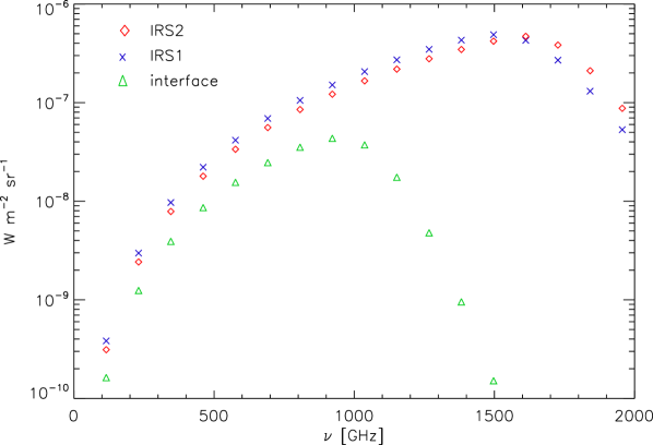
Figure 14: CO ladder from the RADEX fit to the line intensities at the three prominent positions.

Figure 14 shows the resulting CO SED from the RADEX fit for all lines up to $J=17-16$ and Table 8 summarizes the resulting gas parameters. In the fourth column, we translated the CO column density into an equivalent hydrogen column density using the abundance factor of $6\times 10^{-5}$ from Sect.4.1. The higher column density towards IRS 2 compared to that of IRS 1 is driven by the spatial distribution of the low–J CO isotopologues and the high–J CO that is stronger towards IRS 2 (see Fig. 6). The hydrogen column densities towards the two sources approximately match the visual extinction of $A_{\rm V}\approx 50$ towards IRS 1, and $A_{\rm V}\approx 100$ towards IRS 2 measured by Koumpia et al. (2015) when assuming a standard conversion factor of $N_{\rm H}/A_{V}=1.9\times 10^{21}$ cm^-2 (Bohlin et al., 1978).

The IRS 1 and IRS 2 are warmer than the interface and have a similar temperature. The absolute value of the temperature is, however, questionable as it depends on the assumption of the uniform gas parameters within the beam. As discussed already in Sect. 4.1 this also leads to very high densities. The volume density estimates for IRS 1 and IRS 2 are much higher than the ones found in Koumpia et al. (2015) ($\sim$ 10 ⁶ cm^-3) due to the inclusion the high–J CO transitions in the fit (13–12, 16–15). We should rather expect that the different transitions arise from different layers around the infrared sources. The fit produces a good match to all observed lines, so that we have an accurate estimate of the total cooling through all CO lines from the observed sources.

We use again the RADEX gas parameters to compute the C⁺ and oxygen column density from the line intensities given in Table 7. For IRS 1, we get column densities for C⁺ and O of $7\times 10^{17}$ cm^-2 and $1.8\times 10^{18}$ cm^-2, respectively, for IRS 2 $5\times 10^{18}$ cm^-2 cm^-2 and $6\times 10^{18}$ cm^-2 cm^-2. When comparing these values with the map analysis, we notice that the C⁺ column density towards IRS 2 is increased by a factor two because we use the full line width now and extract the intensity exactly at the position of the fine-structure line peak. All other values are basically unchanged. At the interface, we obtain a C⁺ column density of $5\times 10^{18}$ cm^-2 and an oxygen column density of $3\times 10^{19}$ cm^-2. We can compare these values with the column density that we obtain from the total gas column density measured by CO and the upper limits of the abundance of the two species discussed in Sect.4.1. In this way we obtain column densities of $N($C${}^{+})=2\times 10^{18}$ cm^-2 and $N($O$)=5\times 10^{18}$ cm^-2, i.e. much lower than computed here. The explanation must be given by the PDR nature of the cloud interface. As most CO is dissociated there, it is no longer a good measure for the total column density. The actual column density must be at least a factor six higher when using the gas temperature obtained from CO.

4.4 Cooling balance

The ratio of the energy emitted by the interstellar gas in the two main far-infrared cooling lines ([O i] and [C ii]) relative to the integrated far-infrared continuum emitted by the dust can be used to estimate the gas-heating efficiency when assuming that the far-infrared flux reflects the total energy of the incident stellar radiation field by converting it to infrared-wavelengths through absorption and re-emission in an optically thick medium (see e.g. Okada et al., 2013). As access to the [O i] line became possible only very recently, the [C ii]/FIR intensity ratio is often used to measure the efficiency of the gas heating. This allows to address variations in the efficiency of the photoelectric heating from dust grains because photoelectric heating is the most important gas heating process in PDRs (Hollenbach & Tielens, 1999).

Although the definition of the far-infrared varies between different papers (e.g. as FIR integrated from 42 to 122 $\,\mathrm{\mu m}$, or as TIR integrated from 3 to 1100 $\,\mathrm{\mu m}$; Dale & Helou, 2002), the typical range of the gas heating efficiency in Galactic PDRs, star-forming regions in LMC and M33 is $10^{-3}$–$10^{-2}$ both in case of being traced by [O i]$+$[C ii] (Okada et al., 2013; Lebouteiller et al., 2012; Mookerjea et al., 2011; Mizutani et al., 2004) and traced only by [C ii] (Okada et al., 2015; Lebouteiller et al., 2012; Mookerjea et al., 2011). As an extreme case, Vastel et al. (2001) found an efficiency of $10^{-4}$ in W49N, which is illuminated by an intense UV field.

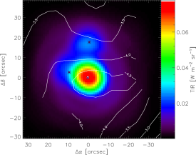
Figure 15: Comparison of the line cooling with the infrared continuum cooling. The background colors show the total infrared flux integrated from wavelengths starting at 11 $\,\mathrm{\mu m}$ (Koumpia et al., 2015). The contours give the decadic logarithm of the ratio of the integrated line flux relative to the continuum flux. In the top panel we use the sum of the [O i] and [C ii] fluxes, in the lower panel, we only show the [C ii]/TIR ratio as used in many existing investigations.

For the region around the embedded sources, the far-infrared luminosity was derived from PACS and SOFIA-FORECAST observations by Koumpia et al. (2015). It was integrated from the observed intensities between 11 and 187 $\,\mathrm{\mu m}$ further extrapolated linearly to zero flux levels at longer wavelengths. Figure 15 compares the energy radiated in our fine structure lines with the total infrared flux ($\lambda>11\,\mathrm{\mu m}$) at the resolution of 13^′′ from the PACS continuum data In the background we see the infrared flux from the three embedded sources with luminosities of 10000 $L_{\odot}$ (IRS 1), 2000 $L_{\odot}$ (IRS 2), and 1300 $L_{\odot}$ (IRS 3), respectively (Koumpia et al., 2015). The contours show the ratio of the sum of the [O i] and [C ii] fluxes relative to the total infrared (upper plot) and the [C ii] line only (lower plot) in logarithmic units.

The [C ii]/TIR ratio shows an almost spherically symmetric picture around IRS 1, being dominated by the variation of the infrared continuum flux. The values of $10^{-3}$–$10^{-2}$, typically observed in other Galactic PDRs, are only seen at the south-western edge of the mapped area closest to the illumination by HD 211880. Around the embedded sources, the infrared luminosity grows without a corresponding growth of the fine-structure line luminosity resulting in [C ii]/TIR ratios below $10^{-5}$ close to IRS 1. The fine structure peak at IRS 2 only weakens this global scenario slightly, resulting in a “dip” in the contours next to IRS 2.

When including the [O i] line in the comparison, the ratio increases by a factor three close to the sources and the fine-structure line peak close to IRS 2 creates a plateau in the energy ratio a about $2\times 10^{-4}$ in agreement to the results obtained in Sect.4.2. At lower densities towards the map boundaries the [O i] contribution is negligible. For IRS 1, even the cooling through the lines of the CO ladder is four times stronger than the sum of the [C ii] and [O i] cooling power (see. Fig. 14), for IRS 2 CO sums up to half of the fine-structure line cooling. Including the CO rotational ladder in the gas cooling budget raises the line-to-continuum ratio to $1-3\times 10^{-4}$, i.e. values that are still extremely small in Galactic context and that would be interpreted as FIR line deficit when observed in external galaxies (e.g. Luhman et al., 1998; Malhotra et al., 2001; Herrera-Camus et al., 2015). However, none of the proposed explanations for the FIR line deficit in external galaxies applies to our case (see Sec. 5).

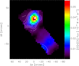
Figure 16: Comparison of the total line cooling flux provided by the sum of the [O i] and [C ii] lines (colors) to the [O i]/[C ii] line flux ratio (contours from 0.4 to 2.8 in steps of 0.4). The computation is performed in a common effective beam of 15^′′.

The ratio between the [O i] and [C ii] intensities is considered as one of the main characteristics of PDRs. For high UV fields, the gas temperature is always above the upper level energy of both transitions so that the ratio between the two lines directly measures the density (Kaufman et al., 1999). However, due to the higher energy of the [O i] transition it falls off quite fast at low UV fields resulting in negligible [O i] cooling for low densities and UV fields (Röllig et al., 2006).

As visible already from Fig. 15, the relative contribution of [O i] and [C ii] to the cooling changes significantly over the cloud. Figure 16 shows the total line cooling budget of the [O i] and [C ii] lines in colors and the [O i]/[C ii] line ratio in contours. We find a relatively constant ratio of 2.5–3 in the whole area of the central cluster connecting IRS 1 and IRS 2. Here, [O i] is dominating the gas cooling. A value of three is representative for either very high UV fields and low densities or low UV fields and very high densities. For the high densities and UV fields around the central cluster, we would however expect much higher values due to the high abundance and emissivity of oxygen in that regime.

When leaving the area of the central cluster, the contribution of [O i] to the total line cooling budget quickly drops off. This should reflect a combination of a reduced density and temperature as measured by CO (Fig. 9). While the density drops more quickly south of IRS 1, the temperature drops more quickly north of IRS 2. The asymmetry of the [O i]/[C ii] ratio plot indicates that the density is the dominating factor here. In the bulk of the cloud and the interface, the cooling strength of the [O i] line can be completely neglected. [C ii] is the only relevant gas cooling line there.

4.5 PDR model interpretation

To overcome the RADEX assumption of constant excitation conditions within the emitting region as an oversimplification we switch to theoretical models for PDR structures that self-consistently compute the temperature and chemical structure of PDR layers around illuminating sources, allowing us to compare the line observations with the model predictions for different densities and radiation fields.

One critical input parameter is the strength of the impinging UV radiation field. It can be computed by assuming that in an optically thick configuration all UV photons are eventually converted into observable infrared photons. Then we obtain the strength of the incident radiation field in terms of the Draine field (Draine, 1978) as:

$$\chi=\frac{I_{\rm TIR}\times 4\pi}{2\times 2.7\times 10^{-6}{\rm W/m^{2}}}$$ (2)

where the factor two in the denominator accounts for half of the heating photons at wavelengths out of the UV band (e.g. Röllig et al., 2011). Using the total infrared flux values from Sect. 4.4 results in $\chi=5.6\times 10^{4}\chi_{0}$ for IRS 2 and $1.2\times 10^{5}\chi_{0}$ for IRS 1. For the interface, the UV field has been derived previously to fall between $140\,\chi_{0}$ (Poelman & Spaans, 2005) and $230\,\chi_{0}$ (Timmermann et al., 1996).

As a simple and straight-forward model, we can treat the PDRs in S 140 as plane-parallel slabs simulated by Kaufman et al. (1999). In the model line and continuum intensities are self-consistently computed for a face-on configuration taking the optical depths of the lines into account. This allows us to directly read the source parameters from the [C ii] line intensity, the [O i]/[C ii] intensity ratio, and the ([O i]+[C ii])/TIR ratio (Figs. 3-6 from Kaufman et al., 1999). As the model has only the two parameters gas density and incident radiation field, the problem is over-determined allowing us to assess the consistency of the description. Depending on the source geometry, we may, however, introduce the inclination angle as an additional free parameter providing a line-of-sight increase of the column densities because the model is only computed for a face-on PDR.

This model is clearly appropriate for the external cloud surface representing an almost edge-on PDR illuminated by HD 211880. The main [C ii] and [O i] emission from a plane-parallel PDR stems from gas within $A_{V}\leq 2$ from the cloud surface (Röllig et al., 2007). This is also the approximate scale of chemical stratification in the PDRs (Hollenbach & Tielens, 1999). In Fig. 2 we can directly measure the stratification between CO 2-1 and [C ii] as 15^′′ or 0.05 pc. This allows to estimate the gas density as $n_{\rm H}\approx 2\times(N_{\rm H}/A_{V})/0.05\;{\rm pc}=2.5\,10^{4}$ cm^-3.

When reading the model predictions for the given parameter combination of density and previously fitted UV field for the interface, we obtain a [C ii] line intensity of $3\times 10^{-7}$ W sr^-1 m^-2, a [O i]/[C ii] energy ratio of 5, and a line-to-continuum ratio of 0.02. Unfortunately, we do not have numbers for the infrared continuum flux at the interface position as it was outside of the region observed by FORECAST and PACS. We can, however, assume that the ([O i]+[C ii])/TIR ratio falls above the value of $10^{-2}$ seen in the south-western edge of the mapped area (Fig. 15). The measured [C ii] line intensity is, however, $10^{-6}$ W sr^-1 m^-2, a value that is obtained in the model only for UV fields above $2\times 10^{4}\chi_{0}$ and high densities. In contrast, the measured [O i](63 $\,\mathrm{\mu m}$)/[C ii] energy ratio is 0.3, a value that is found in the model only for UV fields of about 30 $\chi_{0}$ and below.

A solution can be achieved by introducing the inclination angle of the PDR as additional parameter and changing the assumption on the impinging UV field. If the PDR inclination provides a geometrical magnification of the [C ii] intensity in the optically thin case and we assume that [O i] is optically thick so that it is not amplified in the same way, the observed [C ii] intensity can be corrected downwards and the [O i]/[C ii] ratio upwards. For an amplification factor of eight, we obtain a match of both quantities with the model at a UV field of 60 $\chi_{0}$. This is lower than obtained in the previous PDR model fits, but still six times higher than measured deeper in the S 140 region by Li et al. (2002). Because our gas density value is based on a rough estimate only, we should assume a a factor two error bar for all numbers for a conservative approach. The geometrical amplification of a factor eight is obtained by an inclination angle of 80–85 degrees relative to the face-on orientation. The study of the [O i](145 $\,\mathrm{\mu m}$)/[O i](63 $\,\mathrm{\mu m}$) line ratio based on PACS data in Appx. B suggests a somewhat lower amplification factor of four.

We can try to use the same model as an approximation for the internal PDR around the cluster at IRS 2 that gives rise to the observed [C ii] and [O i] peak. Here, we assume that the PDR will form a shell around the cluster with a face-on front and back side. For the gas density, the value of $1.4\times 10^{5}$ $\,\mathrm{cm^{-3}}$ from Sect. 4.2 provides a lower limit. Reading the observables from the model for this density and the UV field of $5.6\times 10^{4}\chi_{0}$ gives a [C ii] line intensity of $1\times 10^{-6}$ W sr^-1 m^-2, a [O i]/[C ii] energy ratio of 40, and a ([O i]+[C ii])/TIR ratio of $3\times 10^{-3}$. Comparing this to our measured values of $1.5\times 10^{-6}$ W sr^-1 m^-2, 5.6, and $2\times 10^{-4}$ we find a good agreement for the [C ii] line intensity when assuming that the radiation from both surfaces adds up in the optically moderately thick line ($\hat{\tau}=2$, see Sect. 3.1). However, the observed [O i] line intensity and is about seven times lower than predicted resulting in a line-to-continuum ratio that is also six times lower.

The much lower [O i] intensity in the observations may stem from the shell configuration where we expect a decreasing [O i] excitation temperature towards the observer in contrast to the face-on configuration of the PDR model where we directly observe the illuminated side of the PDR. For [C ii] both configurations do not make a big difference as C⁺ is only abundant in the narrow $A_{V}<2$ layer, but atomic oxygen is also abundant in the cool environment at the back side of the PDR, potentially absorbing a large fraction of the [O i] emission from the PDR. If we assume that this self-absorption is as strong as a factor seven, much higher than estimated from the line profiles in Sect. 3.1, we obtain a self-consistent picture for the PDR of IRS 2 in the frame of the PDR model from Kaufman et al. (1999). This self-absorption by a factor of seven is also consistent with the [O i](145 $\,\mathrm{\mu m}$)/[O i](63 $\,\mathrm{\mu m}$) ratio observed by PACS (Appx. B).

By further inspecting the model output as a function of density, we can also constrain the maximum density of the PDR. When increasing the density by a factor ten above our lower limit, the [C ii] intensity drops by a factor two while the predicted [O i] intensity remains approximately constant. In the shell configuration this cannot be compensated by a variable inclination angle so that we can constrain the actual density range to densities below $10^{6}$ $\,\mathrm{cm^{-3}}$. This is consistent with the central density estimate of $9\times 10^{5}$ $\,\mathrm{cm^{-3}}$ from the dust modelling in Koumpia et al. (2015). With the assumption of a very strong [O i] self-absorption, the fine-structure line peak at IRS 2 is thus still consistent with the standard PDR picture in a UV field of $5.6\times 10^{4}\chi_{0}$ and a density between $1.4\times 10^{5}$ and $1\times 10^{6}$ $\,\mathrm{cm^{-3}}$.

However, we do not succeed any more in providing a consistent PDR model explanation for the fine structure line deficit from IRS 1. The combination of the [C ii] intensity of $4\times 10^{-7}$ W sr^-1 m^-2, the [O i]/[C ii] energy ratio of 1.6, the line-to-continuum ratio of $2\times 10^{-5}$, and the known UV field of $1.2\times 10^{5}\chi_{0}$ provides a solution for a gas density of $50$ $\,\mathrm{cm^{-3}}$ and a factor 1.5 self-absorption of the [O i] 63 $\,\mathrm{\mu m}$ line only, but this low density is in clear contradiction to the analysis of the CO lines in Sect. 4.1 and the dust emission profile in Koumpia et al. (2015). In fact, the density around IRS 1 should be at least as high as towards IRS 2.

5 Discussion

Our observational results raise two main questions:

• Why is the fine-structure line cooling from IRS 1 so weak compared to the continuum, with [C ii]/TIR ratios as low as $10^{-5}$?

• Why do we see significantly more fine-structure line emission from the weaker sources IRS 2 compared to IRS 1?

We can discard a number of easy explanations for the lack of [C ii] emission from IRS 1 and the relative weakness of the [O i] and [C ii] emission from IRS 2:

High resolution radio continuum observations using the VLA and MERLIN (Tofani et al., 1995; Hoare, 2006) showed ultracompact H ii regions at the positions of IRS 1 and IRS 2. This shows that the embedded sources produce enough UV photons with energies above 13.6 eV to ionize hydrogen. Therefore, they should also be able to ionize carbon (11.2 eV) and PAHs and dust grains leading to C⁺ production and a significant photoelectric heating of the gas. In the same direction Malhotra et al. (2001) proposed radiation from an older stellar population with an overall redder spectrum to explain the [C ii] deficit, but in our sources we can be sure to find a rather very young cluster.

PACS observations of the [N iii] 57 $\,\mathrm{\mu m}$ line in the frame of the Herschel key project WADI (Ossenkopf et al., 2011) did not provide any detection of the line in $47^{\prime\prime}\times 47^{\prime\prime}$ area centered at IRS 1. Because of the similarity of the second ionization potential of nitrogen and carbon, the lack of N⁺⁺ rules out that carbon is also in the form of C⁺⁺ not contributing to the [C ii] line. Together with the non-detection of the [O iii] line, this rules out that a high ionization parameter explains the lack of [C ii] and [O i] emission. Unfortunately, the existing Spitzer IRS spectra do not allow to constrain the abundance of other ionized species as they are saturated in most of the field due to the large continuum flux. Future observations of infrared lines might show whether there is a general line deficit from the H ii regions that might be due to strong UV absorption by dust within the H ii regions preventing any FUV photons from arriving at the molecular gas around them.

The intensity of the far-infrared lines may be reduced by dust extinction for very large column densities (see e.g. Etxaluze et al., 2013). Mainly constrained by 450 $\,\mathrm{\mu m}$ SCUBA observations we derived in Koumpia et al. (2015) a total visual extinction of $A_{\rm V}\approx 50$ towards IRS 1, and of up to $A_{\rm V}\approx 100$ towards IRS 2. The dust opacities should fall between the values for diffuse clouds (82 cm${}^{2}/g$ at 63 $\,\mathrm{\mu m}$, 12 cm${}^{2}/g$ at 158 $\,\mathrm{\mu m}$, Li & Draine, 2001) and those for dense clumps (211 cm${}^{2}/g$ at 63 $\,\mathrm{\mu m}$, 41 cm${}^{2}/g$ at 158 $\,\mathrm{\mu m}$, Ossenkopf & Henning, 1994, model 5) providing optical depths of $\tau_{\rm 63\,\mathrm{\mu m}}=0.1-0.25$ and $\tau_{\rm 158\,\mathrm{\mu m}}=0.01-0.05$ for IRS 1 and $\tau_{\rm 63\,\mathrm{\mu m}}=0.2-0.5$ and $\tau_{\rm 158\,\mathrm{\mu m}}=0.03-0.2$ for IRS 2 when we assume that half of the dust is located in front of the line-emitting gas. This may provide a reduction of up to 40 % for the [O i] intensity towards IRS 2, but only a negligible effect for all other cases, in particular for the [C ii] line, not explaining the overall large deficiency.

Herrera-Camus et al. (2015) proposed a redistribution of the cooling power from [C ii] to the [O i] 63 $\,\mathrm{\mu m}$ line in dense material as an explanation for the [C ii] deficit, but as we observed both lines, we can be sure that this can only apply for the self-absorbed part of the [O i] line as all other photons are measured. We find, however, a redistribution of cooling power to the CO rotational lines. They can carry as much as half of the energy of the [O i] line, but clearly do not account for a factor 100 difference.

Based on the spatial and spectral information in our data we can exclude a shock-origin of our fine structure peak. It is about 5^′′ apart from the outflow knots from IRS 1 mapped by Weigelt et al. (2002) and the fine-structure lines do not show the outflow wings seen e.g. in [C i] by Minchin et al. (1994) or seen in our low-$J$ CO data. In case of outflow-excited [O i] emission we expect a wider line width in [O i] compared to CO, as observed e.g. in G5.89-0.39 by Leurini et al. (2015) and not the opposite behavior. Moreover, the [O i] line has a slightly blue-skewed profile that is rather representative for infall than for outflow.

In the frame of PDRs, low line-to-continuum cooling ratios are explained by either very high or very low charging parameters $\chi/n$ (e.g. Kaufman et al., 1999). High $\chi/n$ values lead to positively charged dust grains and PAHs, lowering the photoelectric efficiency . They are obtained for very high UV fields at low densities. In the opposite case all material remains cold and no C⁺ is produced so that most energy is emitted in CO lines. However, our CO and dust observations exclude low densities around the infrared sources (Sect. 4.3), the measured [C ii] intensity excludes the cold-gas solution, and the UV fields are constrained by the measured infrared luminosity.

Alternatively, the photoelectric efficiency can be reduced by the destruction of PAHs since PAHs are the dominant carrier of the photoelectric heating (Bakes & Tielens, 1994). As mentioned above, the saturation of the IRS spectra around infrared sources prevent us to examine the PAH spectra directly, but when we compare the relative strength of the PAH 11.3$\,\mathrm{\mu m}$ feature against the underlying continuum southwest of IRS 1, we find some reduction in the area closer area to IRS 1 (20–30^′′ from IRS 1) compared to 30–50^′′ from IRS 1. However, the spectra show still an infrared excess from very small dust grains indicating that the reduction in the PAH abundance can only weakly reduce the overall surface for the photoelectric effect.

The relative weakness of the fine structure lines and the low [O i]/[C ii] ratio must be explained by deviations of the conditions in S 140 from that “standard PDR”. For the [O i] line the low intensity can be explained by a scenario with a decreasing [O i] excitation temperature towards the observer, resulting from a decreasing gas temperature and/or density. Due to the high column density of atomic oxygen at low temperatures, this geometry can provide a strong self-absorption, explaining the factor seven reduction of the [O i] line intensity observed towards IRS 2. However, this mechanism can hardly be responsible for the same kind of reduction in the [C ii] line intensity towards IRS 1. As C⁺ quickly recombines in a dense gas at low temperatures, finally forming CO, we do not expect large quantities of cold C⁺ in the line of sight that can produce the same kind of self-absorption for the [C ii] fine-structure line. A very special configuration would be needed that allows for a significant amount of cold low-density C⁺ gas in a clumpy medium behind a layer of dense and warm gas facing the H ii region around the embedded cluster.

Beyond the relative weakness of the fine-structure lines relative to the continuum flux, we find puzzling combinations of detections:

1. IRS 2, with 2000 $L_{\odot}$ shows strong [O i], [C ii], and CO (and isotopologues) emission at about -6.5 $\,\mathrm{km\,s^{-1}}$ and has associated ultracompact H ii regions.

2. IRS 1, with 10000 $L_{\odot}$ shows only weak [C ii] and [O i] emission at the main velocity of the cloud of -8 $\,\mathrm{km\,s^{-1}}$. The CO lines have a somewhat smaller intensity than on IRS 2 and the optically thin lines are centered at the IRS 2 velocity, showing only an emission wing at -8 kms indicating also a relative lack of CO emission from IRS 1. An ultracompact H ii region and an outflow were detected.

3. IRS 3, with 1300 $L_{\odot}$ shows [O i], but hardly any [C ii], CO is comparable to IRS 1, but spatially not separated in our beam. The source, however shows no associated H ii region.

6 Summary

Our GREAT observations of S 140 showed a pronounced peak of the emission of the [O i] 63 $\,\mathrm{\mu m}$ and [C ii] lines 20^′′ north of IRS 1, the main embedded source dominating the infrared field in the whole region. The fine-structure-line peak can be associated with a weaker infrared source, IRS 2, and the GREAT observations resolve the size of the emitting region to have a diameter of 0.03 pc. The velocity of the gas at that position is offset by about 1.5 $\,\mathrm{km\,s^{-1}}$ from the bulk of the molecular material in S 140. The gas density of the emitting gas must be at least $1.4\times 10^{5}$ $\,\mathrm{cm^{-3}}$ to allow for the observed strength of the [C ii] line. In spite of its absolute strength, the [O i] 63 $\,\mathrm{\mu m}$ line, is however, relatively weak when compared with [C ii] and the infrared continuum. This can only be explained by a strong self-absorption in the foreground medium with a large optical depth. For [C ii] we measured an optical depth of $\hat{\tau}\approx 2$.

From IRS 1 we find only relatively weak [C ii] and almost no [O i] emission in spite of its high luminosity of $10^{4}L_{\odot}$ and a know ultracompact H i region. The main heating source of dust and large scale-gas in S 140 is not responsible for the [C ii] and [O i] peak, but shows an extreme fine-structure line deficit. While for IRS 2, the low value line of the ([C ii]+[O i])/TIR ratio, also matching the criterion for a line deficit, can be explained by the strong [O i] self absorption, this explanation does not work for IRS 1, and in particular not for the low [C ii] intensity observed there. Solving the puzzle of the extremely low fine-structure in S 140 may be the puzzle to a general explanation of the fine-structure line deficit in galaxies with high infrared luminosities.

At the cloud surface of S 140 we find a classical PDR, showing the expected stratification in the line tracers and producing strong [C ii] emission. The [C ii] line is narrower there, having an optical depth of $\hat{\tau}\approx 3$. The combination of the observed stratification and line intensities of [C ii] and [O i] can be explained by a plane-parallel PDR model with a density of $2.5\,10^{4}$ cm^-3 if we assume that the surface is tilted by an inclination angle of 80–85 degrees relative to the face-on orientation and illuminated by a a UV field of 60 $\chi_{0}$, a value that is lower than obtained in the previous PDR model fits in the literature.

Appendix A Comparison to Herschel data

In the frame of the WADI key project (Ossenkopf et al. 2011), S140 was observed with the HIFI and PACS instrument, also covering the [C ii] and [O i] lines. Part of the results were used e.g. in the papers of Dedes et al. (2010) and Koumpia et al. (2015). Due to the limited observing time in the key project only a small part of the source was covered. In the overlapping part we use the data here to check the consistency with our new, more extended observations with GREAT.

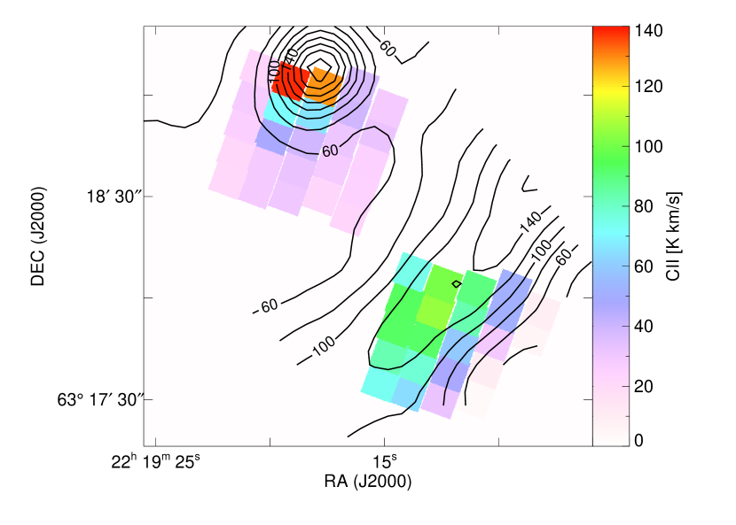
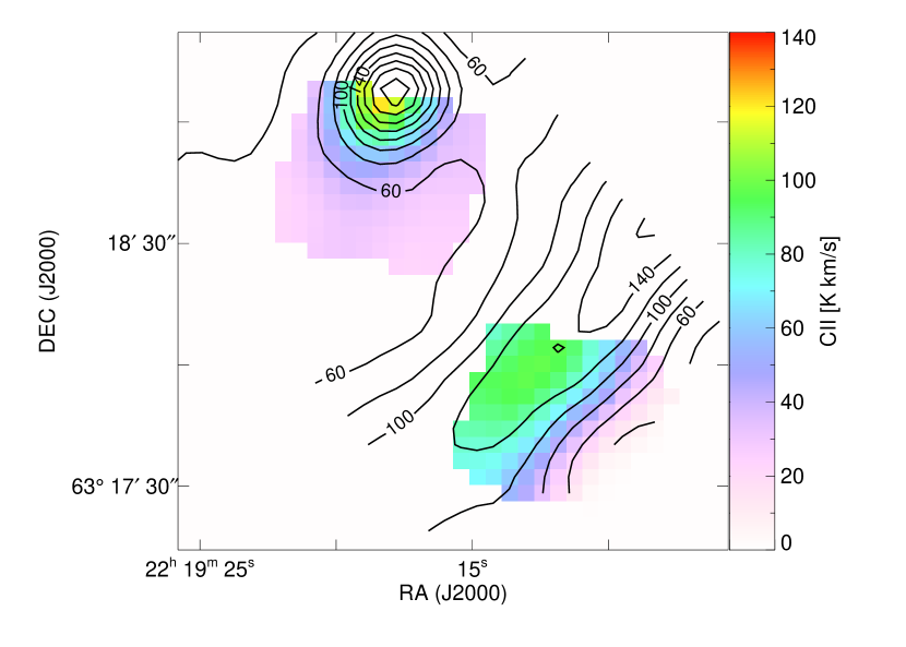
Figure 17: Integrated map of [C ii] obtained in the GREAT observations (contours) overlaid by colors of the [C ii] line intensity from the two PACS footprints. The top image shows the intensities in the original PACS footprints. In the bottom version this is resampled to the positions of the GREAT map with an effective resolution of 17.2^′′ beam.

A.1 PACS spectroscopy

The [O i] and [C ii] lines were observed earlier in S 140 through the PACS instrument onboard Herschel in the frame of a spectral scan at two individual pointing, one centered at IRS 1 and the other one close to the cloud surface towards HD 211880. The PACS footprint is not fully-sampled so that it may miss part of the flux between the pixels, but if we assume a source size of 5.5^′′ or above that missing flux should be small so that we can use the data to check the consistency with the GREAT observations. The spectral resolution of PACS was insufficient to resolve the line, so that we can only compare integrated intensities.

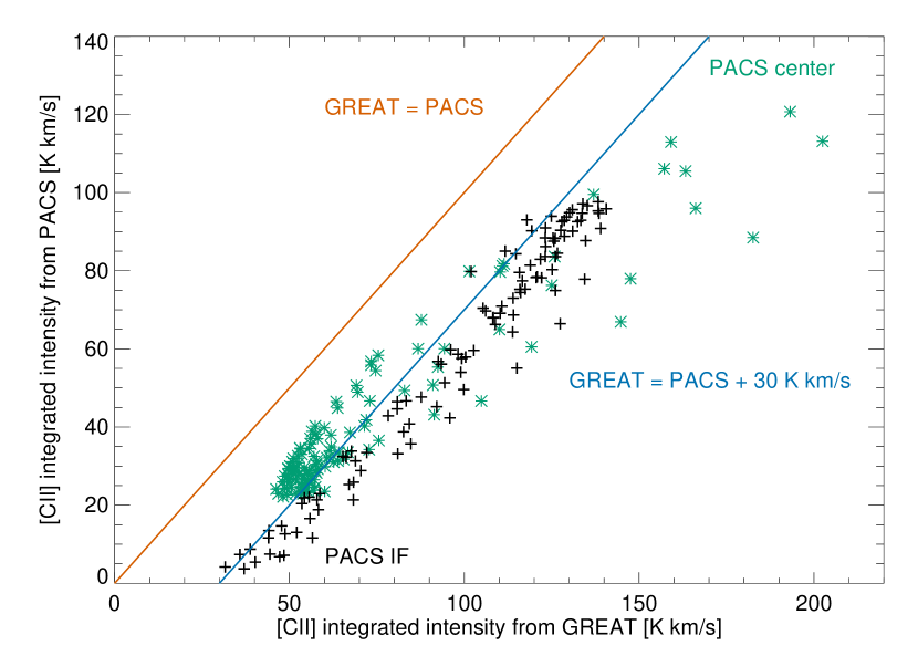
Figure 18: Measured intensities in the different pixels from Fig. 17b as seen by GREAT and PACS. Green asterisks represent the footprint around IRS 1, black plus signs the footprint at the outer interface. The brown line shows the identity, the blue line represent an identity with an offset of 30 K $\,\mathrm{km\,s^{-1}}$.

Figure 17 compares our new intensity map with the PACS data for the two footprints. We see that the spatial structure of the emission peaks around IRS 2 and the interface is consistent between PACS and GREAT data. The PACS data just miss the global emission peak, but they peak at the position closest to the true maximum and they also trace the structure of the extended emission at the outer cloud interface. When comparing absolute intensities, however, we find systematically somewhat lower intensities in the PACS data compared to GREAT data.

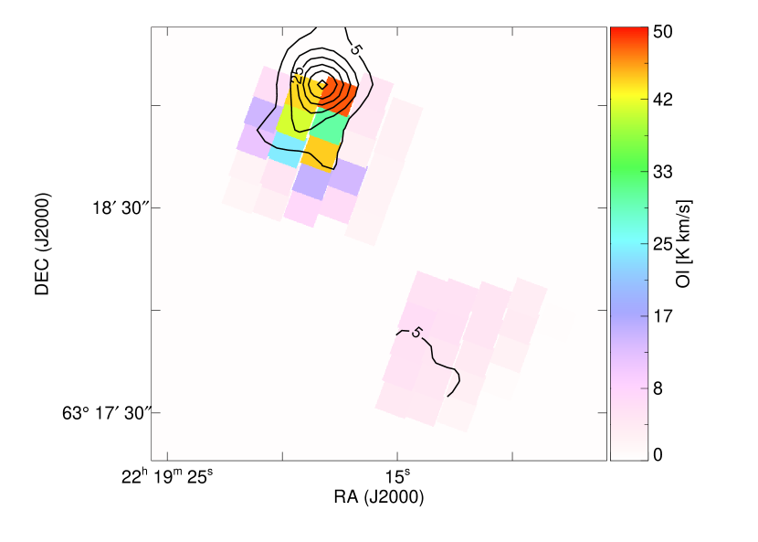
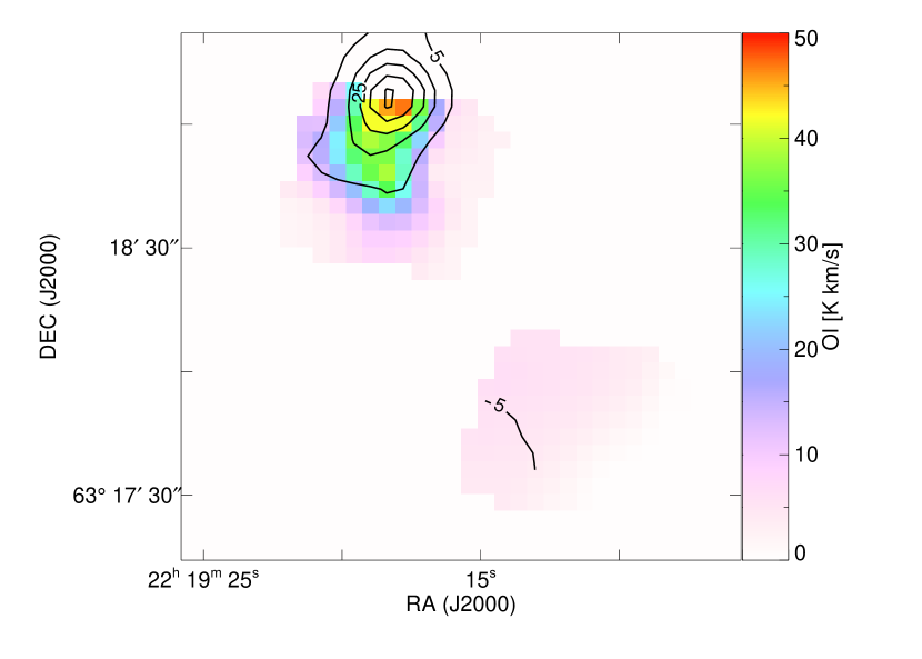
Figure 19: Integrated map of [O i] obtained in the GREAT observations (contours) overlaid colors of the [O i] line intensity from the two PACS footprints. The top image shows the intensities in the original PACS footprints with GREAT data convolved to 10^′′ resolution. In the bottom version both maps are resampled to the positions of the GREAT map for the effective resolution of a circular 12^′′ beam.

To understand whether this is a calibration problem, we computed the pixel-to-pixel statistics in the resampled map. This is shown in Fig. 18. We find a uniform behavior between both footprints; the PACS intensity is offset from the identity by about 30 K $\,\mathrm{km\,s^{-1}}$. This means that we do not have a calibration difference, but a difference in the absolute level. This can be naturally explained if there is a 30 K $\,\mathrm{km\,s^{-1}}$ contamination of the OFF position used as the reference in the PACS observations. The GREAT observations use a well controlled OFF position 6.5^′ south-west of the molecular cloud, while the chopped PACS observations involve a reference that falls 6^′ into the molecular cloud. Some [C ii] emission from that region is quite likely and would explain the constant absolute offset between the GREAT and PACS intensities.

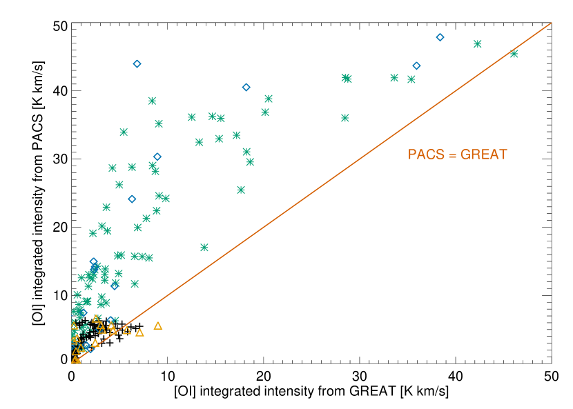
Figure 20: Measured intensities in the different pixels of Fig. 19 as seen by GREAT and PACS. Green asterisks represent the footprint around IRS 1 and black plus signs the footprint at the outer interface when both data sets are resampled to a common 12^′′ resolution (Fig. 19b). Blue diamonds and orange triangles are obtained when we resample instead the GREAT data to the 25 pixels of the PACS array using the 9^′′ PSF of PACS for the IRS 1 region and the interface respectively (Fig. 19a). The brown line shows the identity.

As the [O i] emission is much less extended, we expect no OFF contamination in the PACS data for this line. Figure 19 compares the spatial distribution of the [O i] integrated line emission measured by PACS with our GREAT observations. The spatial distributions of the emission seen through GREAT and PACS agree relatively well, having the peak again around IRS2. But for the individual intensities we find some significant deviations. Fig. 20 compares PACS and GREAT intensities from two different ways of resampling. One is shown in the lower panel of Fig. 19, namely both maps are resampled to a common 4^′′ grid with 12^′′ resolution (green asterisk and black plus sings in Fig. 20). Since the PACS map is not fully-sampled, we extracted the flux based on the geometrical overlap. In the second method, we used the integrated intensity of the original $5\times 5$ PACS spaxels, and resampled the GREAT data to each spaxel position (blue diamonds and orange triangles in Fig. 19. In both ways the resulting trend is the same. There is a good match for the map around the interface and for the highest intensities close to IRS 2 at the northern boundary of the PACS field. However, across the PACS array centered at IRS 1, the intensities seem to by systematically too high. Off-contamination on the GREAT side can be excluded as it would show up as a constant offset like seen in the [C ii] case. Moreover, we used the same reference position as for [C ii] and [O i] is rather less extended than [C ii] due to the higher critical density. On can see in Fig. 20 that the different ways of resampling the data do not make any significant difference. The PACS observer’s manual (v2.3) does not provide any direct explanation. 63$\,\mathrm{\mu m}$ is not listed as a ghost wavelength from other strong emission lines and it is not in the leakage wavelength range. We can only speculate that this may be a stray-light problem where the strong [O i] emission just at the edge of the PACS footprint is partially picked up in the adjacent spaxels. Unfortunately, there are no calibration data available to verify that situation as the calibration observations were not set up to just miss the target. Hence, we cannot provide a quantitative explanation for the mismatch.

A.2 HIFI cut

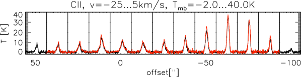
Figure 21: [C ii] spectra taken with HIFI (black) and GREAT (red) along a 37 degrees cut through IRS 1 and the cloud surface. The HIFI cut extends deeper into the cloud and only every second spectrum is plotted. The corresponding GREAT spectra were averaged in a 6^′′ circle around the HIFI position.

The [C ii] line was also observed by HIFI (Dedes et al. 2010) in a single strip going through IRS 1 and the surface also oriented in the same angle of 37 degrees east of north as our GREAT map. In Fig. 21 we compare individual HIFI spectra along that cut at a half-sampled spacing with the corresponding GREAT spectra obtained by averaging all data in a 6^′′ circle around the HIFI positions.

We find a generally very good match between HIFI and GREAT spectra, in particular the line shapes agree in all details, but at some positions the GREAT peak intensities are larger by a few up to 15 %. First of all this confirms the good relative calibration and pointing accuracy of both instruments/telescopes. The higher intensity of GREAT at an offset of $-50^{\prime\prime}$ and $+12^{\prime\prime}$ could be due to the somewhat larger telescope beam of SOFIA leading to more intensity pickup from the surface at $-50^{\prime\prime}$ and from the newly detected intensity peak north of IRS 1 at $+12^{\prime\prime}$.

Appendix B The [O i] 145 $\,\mathrm{\mu m}$/63 $\,\mathrm{\mu m}$ ratio

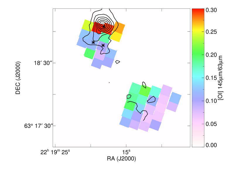
Figure 22: Observed ratio of the [O i] 145 $\,\mathrm{\mu m}$ to [O i] 63 $\,\mathrm{\mu m}$ line integrated intensity seen by PACS (colors) overlaid on the contours of the [O i] 63 $\,\mathrm{\mu m}$ emission measured by GREAT.

In spite of the possible stray-light issue of the PACS [O i] map (see Appx. A.1), we can also try to use the [O i](145 $\,\mathrm{\mu m}$)/[O i](63 $\,\mathrm{\mu m}$) line ratio to constrain the parameters of the PDRs in S 140, assuming that the ratio between both lines should be more robust than the simple integrated line intensity.

Because the excitation energy of the 145 $\,\mathrm{\mu m}$ line of 325 K lies above that of the 63 $\,\mathrm{\mu m}$ line (228 K) the [O i](145 $\,\mathrm{\mu m}$)/[O i](63 $\,\mathrm{\mu m}$) measures temperature (or gas heating through the UV field) in the temperature range of about 300 K. In many cases, however, this ratio may be dominated by the optical depth in the 63 $\,\mathrm{\mu m}$ line (Kaufman et al. 1999; Malhotra et al. 2001). A low [O i](145 $\,\mathrm{\mu m}$)/[O i](63 $\,\mathrm{\mu m}$) compared to the PDR model prediction is observed in many PDRs, and the foreground absorption, opacity effect of the [O i] 63 $\,\mathrm{\mu m}$, and the cloud geometry are proposed as possible explanations (Liseau et al. 1999; Caux et al. 1999; Giannini et al. 2000; Okada et al. 2003). Liseau et al. (2006) provided the theoretical estimates of this ratio for different physical conditions. In case of the optically thin emission, the ratio over 0.1 can be achieved only when the gas temperature is $>500$ K and the collision partner is H₂, which is unlikely. For optically thick case, their calculation with the density of $3\times 10^{4}$ cm^-3 shows that the column density of $N$(H)$>10^{24}$ cm^-2 would be required to make the [O i](145 $\,\mathrm{\mu m}$)/[O i](63 $\,\mathrm{\mu m}$) ratio above 0.1.

Figure 22 shows the integrated intensity ratio of [O i](145 $\,\mathrm{\mu m}$)/[O i](63 $\,\mathrm{\mu m}$) from the two PACS footprints centered at IRS 1 and at the interface observed in the frame of the Herschel key project WADI (Ossenkopf et al. 2011). For the interface parameters discussed above, the face-on PDR model produces a [O i](145 $\,\mathrm{\mu m}$)/[O i](63 $\,\mathrm{\mu m}$) ratio of 0.04, whereas the observed value is 0.17, i.e. about four times higher. If we interpret it through the inclination of the PDR in the same way as for the [C ii] line, the ratio asks for a geometrical amplification of the [O i] 145 $\,\mathrm{\mu m}$ line by a factor four, tow times lower than inferred from the [O i](63 $\,\mathrm{\mu m}$)/[C ii] ratio in Sect. 4.5.

At IRS 2, [O i](145 $\,\mathrm{\mu m}$)/[O i](63 $\,\mathrm{\mu m}$) from PACS observations is 0.3. For the PDR with a UV field of $5.6\times 10^{4}\chi_{0}$ and a density between $1.4\times 10^{5}$ and $10^{6}$ cm^-3 (Sect. 4.5), the predicted ratio is 0.03–0.045. Since the absorption by the cold gas at the back side of the PDR should affect only the 63$\,\mathrm{\mu m}$ transition, a factor 7-10 of self-absorption is required to be consistent with the model predicted [O i](145 $\,\mathrm{\mu m}$)/[O i](63 $\,\mathrm{\mu m}$.

At IRS 1, the observed [O i](145 $\,\mathrm{\mu m}$)/[O i](63 $\,\mathrm{\mu m}$) is 0.1, which suggests the PDR gas with a density of $10^{3}$–$10^{4}$ cm^-3 and a UV field of $>10^{6}$. But as discussed in Sect. 4.5, there is no consistent model for IRS 1.