060006 2014 A. Marti 060006

Using extended Layzer’s potential flow model, we investigate the effects of surface tension on the growth of the bubble and spike in combined Rayleigh-Taylor and Kelvin-Helmholtz instability. The nonlinear asymptotic solutions are obtained analytically for the velocity and curvature of the bubble and spike tip. We find that the surface tension decreases the velocity but does not affect the curvature, provided surface tension is greater than a critical value. For a certain condition, we observe that surface tension stabilizes the motion. Any perturbation, whatever its magnitude, results stable with nonlinear oscillations. The nonlinear oscillations depend on surface tension and relative velocity shear of the two fluids.

Influence of surface tension on two fluids shearing instability

99 inst1 St. Paul’s Cathedral Mission College, 33/1, Raja Rammohan Roy, Sarani, 700 009 Kolkata, India.

1 Introduction

When two different density fluids are divided by an interface, the interface becomes unstable with exponential growth under the action of a constant acceleration acting in the direction perpendicular to the interface from the heavier to lighter fluid or under the action of relative velocity shear of two fluids. These two types of instabilities are known as Rayleigh-Taylor and Kelvin-Helmholtz instabilities, respectively. Temporal development of the nonlinear structure of the interface consequent to Rayleigh-Taylor or Kelvin-Helmholtz instability is currently a topic of interest both from theoretical and experimental points of view. The nonlinear structure is called a bubble if the lighter fluid penetrates across the unperturbed interface into the heavier fluid and it is called a spike if the opposite takes place. The instabilities arise in connection with a wide range of problems ranging from direct or indirect laser driven experiments in the ablation region at compression front during the process of inertial confinement fusion [1, 2] to mixing of plasmas in space plasma systems, such as boundary of planetary magnetosphere, solar wind and cluster of galaxies [3]. In high energy density physics(HEDP), formation of supernova remnant or formation of astrophysical jets [4, 5, 6, 7, 8] are also seen in these types of instabilities. In high energy density plasma experiments using Omega laser [9], Kelvin-Helmholtz instability growth has recently been observed .

There are several methods to describe the nonlinear structure of the interface of two constant density fluids under potential theory and the associated nonlinear dynamics has been studied by many authors [10, 11, 12, 13]. Layzer [10] described the formation of the structure using an expansion near the tip of the bubble or the spike up to second order in the transverse coordinates in two dimensional motion and this approach was extended in Ref. [14] for Kelvin-Helmholtz instability. It is well known [15] that the surface tension reduces the linear Rayleigh-Taylor Growth rate. The lowering in the growth rate is seen to increase with increase in the wave number $k$ up to a critical wave number $k_{c}=\sqrt{\frac{(\rho_{h}-\rho_{l})g}{T}}$, where $T$ denotes surface tension, and $\rho_{h}$ and $\rho_{l}$ are the densities of the heavier and lighter fluids, respectively. The same effect has been described by Mikaelian [16] for Rayleigh–Taylor instability in finite thickness and Sung-Ik Sohn [17] described the effect using the Layzer nonlinear potential model. The nonlinear theory influence of surface tension was elaborately studied by Pullin [18] and Garnier et al. [19] using numerical methods.

The present paper addresses to the problem of the time development of the nonlinear interfacial structure caused by combined Rayleigh–Taylor and Kelvin–Helmholtz instability in presence of surface tension. It is shown that the growth rate of the instabilities is affected by the surface tension. The growth rate of the tip of the bubble or spike are significantly reduced due to the surface tension. We observed an oscillatory stabilization of the interface for large surface tension. This oscillation depends on the relative velocity shear also. Section II deals with the basic hydrodynamical equations together with the geometry involved. Here we assume that the fluids are inviscid and the motion is irrotational. The investigation of the nonlinear aspect of the structure of the two fluids interface is facilitated by Bernoull’s equation together with the pressure balance equation at the interface. The long time asymptotic behavior of the bubble and spike tip for combined Rayleigh–Taylor and Kelvin–Helmholtz instabilities is derived in section III.A and III.B, respectively. We have also discussed the characteristics of the tip of the bubble and the spike derived analytically and numerically. Finally, we have concluded the results in section IV.

2 Basic mathematical model

We have considered two incompressible fluids separated by an interface located at $y=0$ in a two-dimensional $x-y$ plane, where $x$ axis lying normal to the unperturbed fluid interface. The fluid with density $\rho_{h}$ is assumed to overlie the fluid with density $\rho_{l}$ and gravity is taken along negative $y$-axis. In the following discussion, we shall denote the properties of the fluid above the interface by the subscript $h$ and below the interface by the subscript $l$. After perturbation, the nonlinear interface is assumed to take up a parabolic shape, given by

$$y=\eta(x,t)=\eta_{0}(t)+\eta_{2}(t)(x-\eta_{1}(t))^{2}$$ (1)

The perturbed interface forms a bubble or spike according to $\eta_{0}(t)>0$, $\eta_{2}(t)<0$ or $\eta_{0}(t)<0$, $\eta_{2}(t)>0$. Functions $\eta_{0}(t)$ and $\eta_{1}(t)$ are related to the position of the tip of the bubble from the unperturbed interface, i.e, at time $t$ the position of the bubble tip is $(\eta_{1}(t),\eta_{0}(t))$ and $\eta_{2}(t)$ is related to the bubble curvature.

In our previous works [14, 20, 21, 22, 23], we have considered $\eta_{1}(t)=0$ due to the absence of velocity shear parallel to the unperturbed interface. However, in presence of streaming motion of the fluids, the tip of the bubble moves parallel to unperturbed interface with velocity $\dot{\eta_{1}}(t)$.

According to the extended Layzer model [10, 11, 14, 20], the velocity potentials describing the motion for the upper (heavier) and lower (lighter) fluids are assumed to be given by

$$\phi_{h}(x,y,t) =a_{1}(t)\cos{(k(x-\eta_{1}(t))}e^{-k(y-\eta_{0}(t))}$$

$$+a_{2}(t)\sin{(k(x-\eta_{1}(t))}e^{-k(y-\eta_{0}(t))}$$

$$-xU_{h}$$ (2)

$$\phi_{l}(x,y,t) =b_{0}(t)y$$

$$+b_{1}(t)\cos{(k(x-\eta_{1}(t))}e^{k(y-\eta_{0}(t))}$$

$$+b_{2}(t)\sin{(k(x-\eta_{1}(t))}e^{k(y-\eta_{0}(t))}$$

$$-xU_{l}$$ (3)

where $U_{h}$ and $U_{l}$ are streaming velocities of upper and lower fluids, respectively, and $k$ is the perturbed wave number.

The evolution of the interface $y=\eta(x,t)$ can be determined by the kinematical and dynamical boundary conditions. The kinematical boundary conditions are

$$\frac{\partial\eta}{\partial t}-\frac{\partial\eta}{\partial x}\frac{\partial\phi_{h}}{\partial x}=-\frac{\partial\phi_{h}}{\partial y}$$ (4)

$$\frac{\partial\eta}{\partial x}(\frac{\partial\phi_{h}}{\partial x}-\frac{\partial\phi_{l}}{\partial x})=\frac{\partial\phi_{h}}{\partial y}-\frac{\partial\phi_{l}}{\partial y}$$ (5)

and the dynamical boundary condition (first integral of the momentum equation) is of the form

$$-\rho_{h(l)}\frac{\partial\phi_{h(l)}}{\partial t}+\frac{1}{2}\rho_{h(l)}(\vec{\nabla}\phi_{h(l)})^{2}+\rho_{h(l)}gy$$

$$=-p_{h(l)}+f_{h(l)}(t)$$ (6)

The pressure boundary condition at two fluid interface including surface tension [17, 22] is

$$p_{h}-p_{l}=\frac{T}{R}$$ (7)

where $T$ is the surface tension and $R$ is the radius of curvature.

Plugging the condition (7) at the interface $y=\eta(x,t)$ in Eq. (6), we obtain the following equation.

$$\rho_{h}[-\frac{\partial\phi_{h}}{\partial t}+\frac{1}{2}(\vec{\nabla}\phi_{h})^{2}]-\rho_{l}[-\frac{\partial\phi_{l}}{\partial t}+\frac{1}{2}(\vec{\nabla}\phi_{l})^{2}]$$

$$+g(\rho_{h}-\rho_{l})y=-\frac{T}{R}+f_{h}-f_{l}$$ (8)

We have restricted our study near the peak of the perturbed structure where $|k(x-\eta_{1}(t))|\ll 1$. Thus, we can neglect the terms of $O(|x-\eta_{1}|^{i})$ $(i\geq 3)$ [14]. With this point of view, we have

$$\frac{1}{R} =2\eta_{2}\left(1+4\eta_{2}^{2}(x-\eta_{1})^{2}\right)^{-\frac{3}{2}}$$

$$\approx 2\eta_{2}\left(1-6\eta_{2}^{2}(x-\eta_{1})^{2}\right)$$ (9)

We substitute all the parameters $\eta$, $\phi_{h}$ and $\phi_{l}$ in the kinematic and dynamic boundary conditions represented by Eqs. (4), (5), (8) and (9), and equate coefficients of $(x-\eta_{1})^{i}$,$(i=0,1,2)$ and neglect terms $O(|x-\eta_{1}|^{i})$ $(i\geq 3)$. This yields the following equations.

$$\frac{d\xi_{1}}{d\tau}=\xi_{4}$$ (10)

$$\frac{d\xi_{2}}{d\tau}=V_{h}-\frac{\xi_{5}(2\xi_{3}+1)}{2\xi_{3}}$$ (11)

$$\frac{d\xi_{3}}{d\tau}=-\frac{1}{2}(6\xi_{3}+1)\xi_{4}$$ (12)

$$\frac{kb_{0}}{\sqrt{kg}}=-\frac{12\xi_{3}\xi_{4}}{6\xi_{3}-1}$$ (13)

$$\frac{k^{2}b_{1}}{\sqrt{kg}}=\frac{6\xi_{3}+1}{6\xi_{3}-1}\xi_{4}$$ (14)

$$\frac{k^{2}b_{2}}{\sqrt{kg}}=\frac{(2\xi_{3}+1)\xi_{5}-2\xi_{3}(V_{h}-V_{l})}{2\xi_{3}-1}$$ (15)

$$\frac{d\xi_{4}}{d\tau} =\frac{N_{1}(\xi_{3},r)}{D_{1}(\xi_{3},r)}\frac{\xi_{4}^{2}}{(6\xi_{3}-1)}$$

$$+\frac{2(1-r)\xi_{3}(6\xi_{3}-1)}{D_{1}(\xi_{3},r)}\left(1-12\xi_{2}^{2}\frac{k^{2}}{k_{c}^{2}}\right)$$

$$+\frac{N_{2}(\xi_{3},r)}{D_{1}(\xi_{3},r)}\frac{(6\xi_{2}-1)\xi_{5}^{2}}{2\xi_{3}(2\xi_{3}-1)^{2}}$$

$$+\frac{2(4\xi_{3}-1)(6\xi_{3}-1)}{D_{1}(\xi_{3},r)(2\xi_{3}-1)^{2}}$$

$$\times[(V_{h}-V_{l})^{2}\xi_{3}-(V_{h}-V_{l})(2\xi_{3}+1)\xi_{5}]$$ (16)

and

$$\frac{d\xi_{5}}{d\tau} =-\frac{(2\xi_{3}-1)r\xi_{4}\xi_{5}}{2\xi_{3}D_{2}(\xi_{3},r)}$$

$$+\frac{\xi_{4}(6\xi_{3}+1)}{2D_{2}(\xi_{3},r)(6\xi_{3}-1)(2\xi_{3}-1)}$$ (17)

$$\times[4(V_{h}-V_{l})(4\xi_{3}-1)-\frac{\xi_{5}}{\xi_{3}}(28\xi_{3}^{2}-4\xi_{3}-1)]$$

where $r=\frac{\rho_{h}}{\rho_{l}}$; $\xi_{1}=k\eta_{0}$; $\xi_{2}=k\eta_{1}$; $\xi_{3}=\frac{\eta_{2}}{k}$; $\xi_{4}=\frac{k^{2}a_{1}}{\sqrt{kg}}$; $\xi_{5}=\frac{k^{2}a_{2}}{\sqrt{kg}}$; $\tau=t\sqrt{kg}$; $k_{c}^{2}=\frac{(\rho_{h}-\rho_{l})g}{T}$ and $V_{h(l)}=\frac{kU_{h(l)}}{\sqrt{kg}}$ are corresponding dimensionless quantities. The function $N_{1,2}(\xi_{3},r)$ and $D_{1,2}(\xi_{3},r)$ are given by

$$N_{1}(\xi_{3},r)=36(1-r)\xi_{3}^{2}+12(4+r)\xi_{3}+(7-r);$$

$$D_{1}(\xi_{3},r)=12(r-1)\xi_{3}^{2}+4(r-1)\xi_{3}-(r+1)$$ (18)

and

$$N_{2}(\xi_{3},r)=16(1-r)\xi_{3}^{3}+12(1+r)\xi_{3}^{2}-(1+r);$$

$$D_{2}(\xi_{3},r)=2(1-r)\xi_{3}+(r+1)$$ (19)

The temporal development of the combined effect of Rayleigh–Taylor and Kelvin–Helmholtz instability is given by Eqs. (10)–(12), (16) and (17).

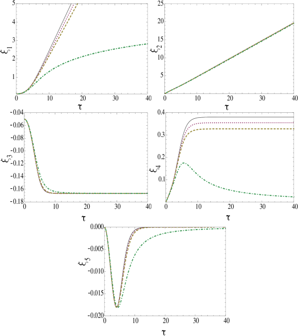
Figure 1: Bubble- variation of $\xi_{1}$, $\xi_{2}$, $\xi_{3}$, $\xi_{4}$ and $\xi_{5}$ with $\tau$. Initial value $\xi_{1}=$0.1, $\xi_{2}=$0, $\xi_{3}=$-0.05, $\xi_{4}=0$, and $\xi_{5}=0$ with $\rho_{h}=3$, $\rho_{l}=2$, $V_{h}$=0.5, $V_{l}=0.1$, $\frac{k^{2}}{k_{c}^{2}}$=0 (line), 0.5 (dot), 1 (dash), 3.9 (dash-dot).

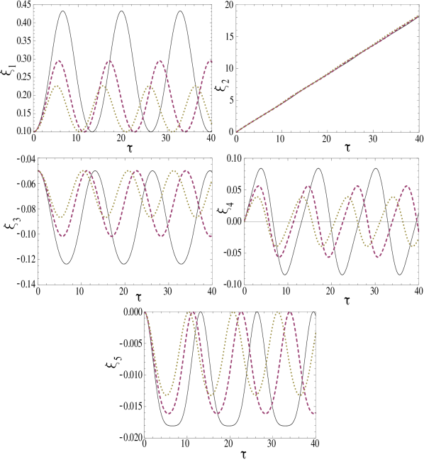
Figure 2: Bubble- variation of $\xi_{1}$, $\xi_{2}$, $\xi_{3}$, $\xi_{4}$ and $\xi_{5}$ with $\tau$. Initial value $\xi_{1}=$0.1, $\xi_{2}=$0, $\xi_{3}=$-0.05, $\xi_{4}=0$, and $\xi_{5}=0$ with $\rho_{h}=3$, $\rho_{l}=2$, $V_{h}$=0.5, $V_{l}=0.1$, $\frac{k^{2}}{k_{c}^{2}}$=10 (line), 15 (dot), 20 (dash).

Figure 3: Bubble- variation of $\xi_{1}$, $\xi_{2}$, $\xi_{3}$, $\xi_{4}$ and $\xi_{5}$ with $\tau$. Initial value $\xi_{1}=$0.1, $\xi_{2}=$0, $\xi_{3}=$-0.05, $\xi_{4}=0$, and $\xi_{5}=0$ with $\rho_{h}=3$, $\rho_{l}=2$, $\frac{k^{2}}{k_{c}^{2}}$=20, $V_{h}$=0, $V_{l}=0$ (line), $V_{h}$=0.5, $V_{l}=0.1$(dot), $V_{h}$=1, $V_{l}=0.1$ (dash), $V_{h}$=1.5, $V_{l}=0.1$ (dash-dot).

3 Numerical results and discussions

3.1 Effect of surface tension on bubble growth

In this section, we present the effect of surface tension on the nonlinear growth rate of the bubble tip for combined Rayleigh–Taylor and Kelvin–Helmholtz instability. To describe the dynamics of the bubble tip, it is essential to integrate Eqs. (10)–(12), (15) and (16) by numerical simulation. To obtain the initial conditions of the numerical integration, we assume that the initial interface is given by $y=\eta_{0}(t=0)cos(kx)$. The expansion of the cosine function gives $(\xi_{2})_{initial}=0$ and $(\xi_{3})_{initial}=-\frac{1}{2}(\xi_{1})_{initial}$, where $(\xi_{1})_{initial}$ is the arbitrary initial amplitude. Since the perturbation starts from rest, we may often choose $(\xi_{4})_{initial}=(\xi_{5})_{initial}=0$. The non-dimensionalized time development plots of $\xi_{1}$, $\xi_{2}$, $\xi_{3}$,$\xi_{4}$ and $\xi_{5}$ are shown in Figs. 1, 2 and 3.

Before we describe the nature of the bubble tip, consider the asymptotic behavior of the tip. As $\tau\rightarrow\infty$, the asymptotic values of $\xi_{3}$, $\xi_{4}$ and $\xi_{5}$ for bubble are obtained by setting $\frac{d\xi_{3}}{d\tau}=0$, $\frac{d\xi_{4}}{d\tau}=0$ and $\frac{d\xi_{5}}{d\tau}=0$. Note that, if $k^{2}<3\left(1+\frac{15}{16}\frac{\rho_{l}}{\rho_{h}-\rho_{l}}(\Delta V)^{2}\right)k_{c}^{2}$, where $\Delta V=V_{h}-V_{l}$, the asymptotic values are

$$[(\xi_{3})_{asymp}]_{bubble}=-\frac{1}{6}$$ (20)

$$[(\xi_{4})_{asymp}]_{bubble}$$ (21)

$$=\sqrt{\frac{2A}{3(1+A)}\left(1-\frac{k^{2}}{3k_{c}^{2}}\right)+\frac{5}{16}\frac{1-A}{1+A}(\Delta V)^{2}}$$

and

$$[(\xi_{5})_{asymp}]_{bubble}=0$$ (22)

where, $A=\frac{\rho_{h}-\rho_{l}}{\rho_{h}+\rho_{l}}$ is the Atwood number.

It is clear form Fig. 1 that surface tension suppresses the velocity and growth of the bubble tip significantly, provided surface tension is larger than a critical threshold, $T<T_{c}^{bubble}$, where

$$T_{c}^{bubble}=3\left((\rho_{h}-\rho_{l})+\frac{15}{16}\rho_{l}(\Delta V)^{2}\right)\frac{g}{k^{2}}$$ (23)

Here the critical value depends on the magnitude of relative velocity shear of two fluids and the growth and velocity of the tip reduced if $T<T_{c}^{bubble}$.

When there is no tangential velocity difference (i.e., $V_{h}=V_{l}$) between the two fluids initially, the fluids are purely prone to the Rayleigh–Taylor instability and the critical value becomes $\frac{3(\rho_{h}-\rho_{l})g}{k^{2}}$. These results agree with the argument in Ref. [17]. In absence of surface tension, the asymptotic values coincide with the results obtained in our previous work [14].

Further, if $T>T_{c}^{bubble}$ , oscillatory state emerges even for $r>1$. Figures 2 and 3 describe the oscillatory state of the motion. The amplitude and the period of oscillation decrease monotonically for large surface tension (Fig. 2), while the amplitude of oscillation increases for large relative velocity shear (Fig. 3). In this respect, Figs. 2 and 3 show that there always exists a self generated oscillatory transverse velocity component ($-\xi_{5}$) due to perturbation and this depends upon surface tension as well as the relative velocity shear $\Delta V$ at the two fluids interface. For negative velocity shear (i.e, $\Delta V<0$), the self generated oscillatory transverse velocity of the bubble peak acts opposite to the direction of $V_{h}$ and the amplitude of oscillation increases for large surface tension.

If $T=T_{c}^{bubble}$, equilibrium is attained, i.e,

$$\dot{\xi}_{3}=\dot{\xi}_{4}=\dot{\xi}_{5}=0$$

$$\mbox{ when }\xi_{3}=-\frac{1}{6}\mbox{ and }\xi_{4}=\xi_{5}=0$$ (24)

and the equilibrium becomes unstable. This feature is shown with a dot-dash line in Fig. 1. Thus, the combined Rayleigh–Taylor and Kelvin–Helmholtz instability is stabilized when

$$k^{2}>3\left(1+\frac{15}{16}\frac{\rho_{l}}{\rho_{h}-\rho_{l}}(\Delta V)^{2}\right)k_{c}^{2},$$

$$\mbox{i.e., }T>T_{c}^{bubble}$$ (25)

while the instability however persists but with reduced growth rate for

$$k^{2}\leq 3\left(1+\frac{15}{16}\frac{\rho_{l}}{\rho_{h}-\rho_{l}}(\Delta V)^{2}\right)k_{c}^{2},$$

$$\mbox{i.e., }T\leq T_{c}^{bubble}$$ (26)

According to the condition (25), for $\rho_{h}=3$, $\rho_{l}=2$, $V_{h}=0.5$ and $V_{l}=0.1$, the motion is stabilized when $\frac{k^{2}}{k_{c}^{2}}>3.9$. These results are exhibited in Fig. 2, where $\frac{k^{2}}{k_{c}^{2}}>3.9$. For $\frac{k^{2}}{k_{c}^{2}}=3.9$, the growth rate of the instability is asymptotically diminished and becomes $0$ (dash-dot line of Fig. 1). However, Fig. 1 shows the suppression of growth rate of the instability due to surface tension, when $\frac{k^{2}}{k_{c}^{2}}<3.9$.

Figure 4: Spike- variation of $\xi_{1}$, $\xi_{2}$, $\xi_{3}$, $\xi_{4}$ and $\xi_{5}$ with $\tau$. Initial value $\xi_{1}=$-0.1, $\xi_{2}=$0, $\xi_{3}=$0.05, $\xi_{4}=0$, and $\xi_{5}=0$ with $\rho_{h}=3$, $\rho_{l}=2$, $V_{h}$=0.5, $V_{l}=0.1$, $\frac{k^{2}}{k_{c}^{2}}$=0 (line), 0.5 (dot), 1 (dash), 4.35 (dash-dot).

Figure 5: Spike- variation of $\xi_{1}$, $\xi_{2}$, $\xi_{3}$, $\xi_{4}$ and $\xi_{5}$ with $\tau$. Initial value $\xi_{1}=$-0.1, $\xi_{2}=$0, $\xi_{3}=$0.05, $\xi_{4}=0$, and $\xi_{5}=0$ with $\rho_{h}=3$, $\rho_{l}=2$, $V_{h}$=0.5, $V_{l}=0.1$, $\frac{k^{2}}{k_{c}^{2}}$=10 (line), 15 (dot), 20 (dash).

3.2 Effect of surface tension on spike growth

The temporal evolution of spike state is exhibited in Figs. 4, 5 and 6; the results follow from the numerical integration of Eqs. (10)–(12), (15) and (16) using the transformation $\xi_{1}\rightarrow-\xi_{1}$, $\xi_{3}\rightarrow-\xi_{3}$, $g\rightarrow-g$, $r\rightarrow\frac{1}{r}$ and $V_{h}\rightleftharpoons V_{l}$. The saturation curvature and velocity of the spike tip are given by

$$[(\xi_{3})_{asymp}]_{spike}=\frac{1}{6}$$ (27)

$$[(\xi_{4})_{asymp}]_{spike}$$ (28)

$$=\sqrt{\frac{2A}{3(1-A)}\left(1-\frac{k^{2}}{3k_{c}^{2}}\right)+\frac{5}{16}\frac{1+A}{1-A}(\Delta V)^{2}}$$

and

$$[(\xi_{5})_{asymp}]_{spike}=0$$ (29)

provided $k^{2}<3\left(1+\frac{15}{16}\frac{\rho_{h}}{\rho_{h}-\rho_{l}}(\Delta V)^{2}\right)k_{c}^{2}$.

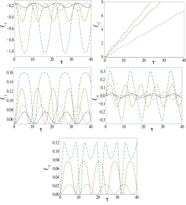
Figure 6: Spike- variation of $\xi_{1}$, $\xi_{2}$, $\xi_{3}$, $\xi_{4}$ and $\xi_{5}$ with $\tau$. Initial value $\xi_{1}=$-0.1, $\xi_{2}=$0, $\xi_{3}=$0.05, $\xi_{4}=0$, and $\xi_{5}=0$ with $\rho_{h}=3$, $\rho_{l}=2$, $\frac{k^{2}}{k_{c}^{2}}$=20, $V_{h}$=0, $V_{l}=0$ (line), $V_{h}$=0.5, $V_{l}=0.1$ (dot), $V_{h}$=1, $V_{l}=0.1$ (dash), $V_{h}$=1.5, $V_{l}=0.1$ (dash-dot).

Figure 4 describes that large surface tension suppresses the growth rate of the spike tip, as well as the bubble. The nonlinear oscillation of the spike tip is observed for $k^{2}>3\left(1+\frac{15}{16}\frac{\rho_{h}}{\rho_{h}-\rho_{l}}(\Delta V)^{2}\right)k_{c}^{2}$ and the equilibrium state arises when equality holds. The pattern of amplitude and period of oscillation are identical to that for the bubble (Figs. 5 and 6). Figure 5 shows the oscillatory behavior of the spike structure for different values of surface tension while the dependency of the relative velocity shear is demonstrated in Fig. 6.

4 Conclusion

In this paper, we have studied a potential flow model to describe the nature of the nonlinear structure of a two-fluid interface under the combined action of Rayleigh–Taylor and Kelvin–Helmholtz instabilities due to surface tension. The analytic expressions for bubble and spike growth rates at asymptotic stage are obtained for arbitrary Atwood number and velocity shear. Surface tension becomes a stabilizing factor of the instability, provided it is larger than a critical value. In this case, oscillatory behavior of motion described by numerical integration of governing equations. The nature of oscillations depends on both surface tension and relative velocity shear of two fluids. On the other hand, below the critical value, surface tension dominates the growth and growth rate of the instability. This result is expected to improve the understanding of the stabilization factor for the astrophysical instability.

- [1] D K Bradley, D G Barun, S G Glendinning, M J Edwards, J L Milovich, C M Sorce, G W Collins, S W Hann, R H Page, R J Wallace, Very-high-growth-factor planar ablative Rayleigh–Taylor experiments, Phys. Plasmas 14, 056313 (2007).
- [2] K S Budil, B A Remington, T A Peyser, K O Mikaelian, P L Miller, N C Woolsey, W M Wood-Vasey, A M Rubenchik, Experimental comparison of classical versus ablative Rayleigh–Taylor instability, Phys. Rev.Lett. 76, 4536 (1996).
- [3] H Hasegawa, M Fujimoto, T-D Phan, H Reme, A Balogh, M W Dunlop, C Hashimoto, R TanDokoro, Transport of solar wind into Earth’s magnetosphere through rolled-up Kelvin–Helmholtz vortices, Nature 430, 755 (2004).
- [4] R P Drake, Hydrodynamic instabilities in astrophysics and in laboratory high-energy–density systems, Plasma Phys. Control. Fusion 47, B419 (2005).
- [5] J O Kane, H F Robey, B A Remington, R P Drake, J Knauer, D D Ryutov, H Louis, R Teyssier, O Hurricane, D Arnett, R Rosner, A Calder, Interface imprinting by a rippled shock using an intense laser, Phys. Rev. E 63, 055401R (2001).
- [6] D D Ryutov, B A Remington, Scaling astrophysical phenomena to high-energy-density laboratory experiments, Plasma Phys. Control. Fusion 44, B407 (2002).
- [7] L Spitzer, Behavior of matter in space, Astrophys. J. 120, 1 (1954).
- [8] B A Remington, R P Drake, H Takabe, D Arnett, A review of astrophysics experiments on intense lasers, Phys. Plasma 7, 1641 (2000).
- [9] E C Harding, J F Hansen, O A Hurricane, R P Drake, H F Robey, C C Kuranz, B A Remington, M J Bono, M J Grosskopf, R S Gillespie, Observation of a Kelvin–Helmholtz instability in a high-energy-density plasma on the omega laser, Phys. Rev.Lett. 103, 045005 (2009).
- [10] D Layzer, On the Instability of Superposed Fluids in a Gravitational Field, Astrophys. J. 122, 1 (1955).
- [11] V N Goncharov, Analytical model of nonlinear, single-mode, classical Rayleigh–Taylor instability at arbitrary Atwood numbers, Phys. Rev. Lett. 88, 134502 (2002).
- [12] Sung-Ik Sohn, Simple potential-flow model of Rayleigh–Taylor and Richtmyer–Meshkov instabilities for all density ratios, Phys. Rev. E 67, 026301 (2003).
- [13] Q Zhang, Analytical solutions of Layzer-type approach to unstable interfacial fluid mixing, Phys. Rev. Lett. 81, 3391 (1998).
- [14] R Banerjee, L Mandal, M Khan, M R Gupta, Effect of viscosity and shear flow on the nonlinear two fluid interfacial structures, Phys. Plasmas 19, 122105 (2012).
- [15] S Chandrasekhar, Hydrodynamic and hydromagnetic stability, Dover, New York (1961).
- [16] K O Mikaelian, Rayleigh–Taylor instability in finite-thickness fluids with viscosity and surface tension, Phys. Rev. E 54, 3676 (1996).
- [17] Sung-Ik Sohn, Effects of surface tension and viscosity on the growth rates of Rayleigh–Taylor and Richtmyer–Meshkov instabilities, Phys. Rev. E 80, 055302(R) (2009).
- [18] D I Pullin, Numerical studies of surface tension effects in nonlinear Kelvin–Helmholtz and Rayleigh–Taylor instability, J. Fluid Mech. 119, 507 (1982).
- [19] J Garnier, C Cherfils-Clerouin, A P Holstein, Statistical analysis of multimode weakly nonlinear Rayleigh–Taylor instability in the presence of surface tension, Phys. Rev. E 68, 036401 (2003).
- [20] R Banerjee, L Mandal, S Roy, M Khan, M R Gupta, Combined effect of viscosity and vorticity on single mode Rayleigh–Taylor instability bubble growth, Phys. Plasmas 18, 022109 (2011).
- [21] M R Gupta, R Banerjee, L K Mandal, R Bhar, H C Pant, M Khan, M K Srivastava, Effect of viscosity and surface tension on the growth of Rayleigh–Taylor instability and Richtmyer–Meshkov instability induced two fluid interfacial nonlinear structure, Indian J. Phys. 86, 471 (2012).
- [22] R Banerjee, L Mandal, M Khan, M R Gupta, Bubble and spike growth rate of Rayleigh Taylor and Richtmeyer Meshkov instability in finite layers, Indian J. Phys. 87, 929 (2013).
- [23] R Banerjee, L Mandal, M Khan, M R Gupta, Spiky Development at the Interface in Rayleigh–Taylor Instability: Layzer Approximation with Second Harmonic, J. Morden Phys. 4, 174 (2013).