Analytic models of the Rossiter-McLaughlin effect for arbitrary eclipser/star size ratios and arbitrary multiline stellar spectra

Abstract

We present an attempt to improve models of the Rossiter-McLaughlin effect by relaxing several restrictive assumptions. We consider the entire multiline stellar spectrum rather than just a single line, use no assumptions about the shape of the lines profiles, and allow arbitrary size ratio for the star and its eclipser. However, we neglect the effect of macro-turbulence and differential rotation. We construct our model as a power series in the stellar rotation velocity, $V\sin i$, giving a closed set of analytic formulae for up to three terms, and assuming quadratic limb-darkening law. We consider three major approaches of determining the Doppler shift: cross-correlation with a predefined template, cross-correlation with an out-of-transit stellar spectrum, and parametric modelling of the spectrum.

A numerical testcase revels that our model preserves good accuracy for the rotation velocity of up to the limit of $2-3$ times the average linewidth in the spectrum. We also apply our approach to the Doppler data of HD 189733, for which we obtain an improved model of the Rossiter-McLaughlin effect with two correction terms, and derive a reduced value for $V\sin i$.

1 Introduction

Whereas the number of the discovered exoplanets grows continuously, the importance of their cross-characterization by independent observation techniques increases. There are two mostly productive planet detection methods: by radial velocity (RV) variations and by a photometric fadening during a transit. Consequently, the joint analysis of the combined RV+transit data gained a special value in the recent years.

This task is not reduced to a mere combination of the RV and transit data, with their respective separate models. In such cases we may also observe hybrid events, like the Rossiter-McLaughlin (RM) effect, which is basically a spectrosopic view of a planetary transit before a rotating star.

The most simple model of this effect is based on the assumption that the measured Doppler anomaly is equal to the average RV of the occulted stellar disk (Kopal, 1942; Ohta et al., 2005; Giménez, 2006). We will call this as classic RM model. This average velocity is given by an exact formula

$$V_{\mathrm{mean}}=-\frac{fv_{\mathrm{p}}}{1-f},$$ (1.1)

where $f$ is a fraction of the flux blocked by the planet, and $v_{\mathrm{p}}$ is the average “subplanet” RV, computed with an account for the stellar limb darkening. The remaining problem here is to compute $f$ and $v_{\mathrm{p}}$ for an assumed limb-darkening law. However, $V_{\mathrm{mean}}$ in this formula is not the same physical quantity as the Doppler anomaly that we seek. Instead of averaging the RV over the stellar disk, we must average the stellar spectrum first, and then determine the Doppler anomaly from this average spectrum.

The average of a function is not equal to the function of an averaged argument, unless the function is linear or well-linearizable. Therefore, the formulae (1.1) approximates the RM anomaly only if the stellar rotation velocity $V\sin i$ is very small. Ideally, it should be much smaller than the typical width of the spectral lines (scaled in the velocity units). In this case, stellar spectrum can be linearized with respect to the rotational Doppler shift. In the remaining cases, the formula (1.1) cannot be used to predict the RM anomaly, with enough accuracy at least.

There are works in which an attempt is made to construct more accurate approximation than (1.1), see e.g. (Hirano et al., 2010, 2011; Boué et al., 2013). They succeeded a lot in this field, but the problem is still far from being solved due to some restrictive asumptions adopted by these authors. A major one is that their analytic results refer to a simplified single-line model of the stellar spectra. In practice, however, Doppler shift is determined from rich spectra that contain thousands of lines or more. Assumption of a single line cannot leave no implications on the reliability of the model. Another important assumptions are that line profiles should be symmetric (Boué et al., 2013) and the planet is assumed small in all these works.

Our aim here is to consider the full stellar spectrum containing multiple lines, and discuss the differences with a single-line model. Also, we tried to avoid decompositions in planet radius, whenever possible. This may be useful for red dwarfs transited by a giant planet. In this case, the planet/star radii ratio may exceed $1/10$. As far as we could learn, the largest or one of the largest values for this ratio currently belongs to the unique circumbinary planet KIC 9632895 (Welsh et al., 2015). Here this ratio reaches $0.26$ for one of the binary components, although the absolute planet radius is only $6.2R_{\earth}$. In theory, a red dwarf star can be even smaller than a giant planet, so such a ratio can even be comparable to or exceed unit.

The structure of the paper is summarized as follows. In Sect. 2 we give general mathematical formulation and present several methods and main formulae that are useful for analytic modelling the RM effect under different assumptions. In Sect. 3 we derive our main results of the RM effect. In Sect. 4 we describe an analytic computation of the RV momenta in an occulted stellar disk, which appear in our RM model. In Sect. 5 we present results of a simulation to test the accuracy and usefullness of the model. In Sect. 6 we apply our models of the RM effect to the public data of the MS star HD 189733, using it as a testcase.

2 Main mathematical methods and techniques for modelling the Rossiter-McLaughlin anomaly

2.1 General formulae and definitions

Let us adopt the logarithmic scale in the wavelength, $s=\ln\lambda$, and denote the spectrum of the star surface near the disk centre as $\mathcal{F}(s)$. The Doppler-shifted spectrum should then be $\mathcal{F}(s-\tau)$, where the Doppler shift is $\tau=v_{z}/c+\mathcal{O}(v^{2}/c^{2})$, with $v_{z}$ being the radial velocity of an emitting point (the $z$ axis directed along the line of sight). This is a non-relativistic approximation. Light coming from different points in the visible stellar disk is combined with different Doppler shifts and different local brightness, forming two auxiliary spectra: the cumulative star spectrum $\mathcal{F}_{\star}(s)$ and the “subplanet” spectrum $\mathcal{F}_{\mathrm{p}}(s)$, which is generated by a portion of the surface blocked by the transiting object. These spectra can be expressed as follows:

$$\mathcal{F}_{\star}(s)=\int\limits_{|\textbf{{R}}|<1}\mathcal{F}(s-\upsilon x)I(|\textbf{{R}}|,s)d\textbf{{R}},\qquad\mathcal{F}_{\mathrm{p}}(s)=\int\limits_{\mathcal{S}_{\mathrm{p}}}\mathcal{F}(s-\upsilon x)I(|\textbf{{R}}|,s)d\textbf{{R}},\qquad\qquad\textbf{{R}}=\{x,y\}.$$ (2.1)

where $\upsilon=\frac{V\sin i}{c}$ is a renormalized rotation velocity, $I(R,s)$ is the limb-darkening law normalized to $I(0)=1$. This law may depend on the wavelength. The integration is done either over the entire star disk $|\textbf{{R}}|<1$ or over the subplanet portion of the disk $\mathcal{S}_{\mathrm{p}}$. The star radius is assumed unit here, meaning that radial velocity of each point of the surface is equal to just $\upsilon x$. The observed star spectrum during a transit is then expressed as $\mathcal{F}_{\mathrm{t}}(s)=\mathcal{F}_{\star}(s)-\mathcal{F}_{\mathrm{p}}(s)$. The formulae (2.1) assume that their integrad does not depend on the point in the stellar disk, except for via the rotational Doppler shift and limb darkening law that may vary with wavelength. Some effects may induce additional changes. For example, macro-turbulence in the stellar atmosphere makes lines characteristics different in the disk centre and near the limb due to different projected geometry of the turbulent motions (e.g. Hirano et al., 2011; Boué et al., 2013). Here we do not take into account effects of this type.

From (2.1), the spectrum of a non-rotating star would be

$$\mathcal{F}_{\star}^{0}(s)=\mathcal{F}(s)\int\limits_{|\textbf{{R}}|<1}I(|\textbf{{R}}|,s)d\textbf{{R}},$$ (2.2)

which slightly differs from the surface spectrum $\mathcal{F}(s)$ due to the wavelength dependence of the limb-darkening law. However, the multiplier near $\mathcal{F}$ is a slowly varying function, so in practice the difference between $\mathcal{F}_{\star}^{0}$ and $\mathcal{F}$ is not important. Below, we will often say “non-rotating star spectrum” actually meaning $\mathcal{F}$.

Contrary to Boué et al. (2013), we do not make an assumption that $\mathcal{F}(s)$ contains only a single line, and also we honor the dependence of the limb-darkening law on the spectral range. Concerning the notations, we do not introduce an explicit Doppler shift to the argument of $\mathcal{F}_{\mathrm{p}}$ at this stage, and we do not normalize our spectra to unit.

2.2 Modelling the procedure of determining the Doppler shift from the spectrum

Now assume that we have a comparison, or template, spectrum $\mathcal{F}_{\mathrm{T}}(s)$ and seek the best fitting Doppler shift by minimizing the goodness-of-fit function as follows:

$$\chi^{2}(\hat{s},a)=\int\limits_{-\infty}^{+\infty}\left(\mathcal{F}_{\mathrm{t}}(s)-a\mathcal{F}_{\mathrm{T}}(s-\hat{s})\right)^{2}ds\longmapsto\min_{\hat{s},a}.$$ (2.3)

From now on, let us introduce the scalar product of functions $\langle f,g\rangle$ and the norm $||f||^{2}$ in the sense of the $L_{2}$ metric. With these definitions we may write the following:

$$\chi^{2}(\hat{s},a)=||\mathcal{F}_{\mathrm{t}}||^{2}-2a\left\langle\mathcal{F}_{\mathrm{t}}(s)\mathcal{F}_{\mathrm{T}}(s-\hat{s})\right\rangle+a^{2}||\mathcal{F}_{\mathrm{T}}||^{2}.$$ (2.4)

The first and the third terms here do not depend on $\hat{s}$, so to fit $\hat{s}$ means to maximize the cross-correlation function (CCF):

$$C_{\mathrm{tT}}(\hat{s})=\left\langle\mathcal{F}_{\mathrm{t}}(s)\mathcal{F}_{\mathrm{T}}(s-\hat{s})\right\rangle\longmapsto\max_{\hat{s}}\quad\implies\quad\left\langle\mathcal{F}_{\mathrm{t}}(s)\mathcal{F}_{\mathrm{T}}^{\prime}(s-\hat{s})\right\rangle=0.$$ (2.5)

Note that without loss of generality we may assume that CCF of $\mathcal{F}_{\star}$ with $\mathcal{F}_{\mathrm{T}}$ is maximized at $\hat{s}=0$, implying that

$$\left\langle\mathcal{F}_{\star}\mathcal{F}_{\mathrm{T}}^{\prime}\right\rangle=0.$$ (2.6)

This means that the template $\mathcal{F}_{\mathrm{T}}$ is centred so that for an uneclipsed star the fitted RV is zero, and during the transit we deal with only the RV offset due to the RM effect.

The comparison template $\mathcal{F}_{\mathrm{T}}$ may be either an a priori given mask, or we may adopt it be equal to the uneclipsed star spectrum $\mathcal{F}_{\mathrm{T}}=\mathcal{F}_{\star}$. Up to a certain degree, these cases model the classic CCF approach, and to the iodine cell technique of Doppler measurements, respectively (Hirano et al., 2010, 2011; Boué et al., 2013). Note that Boué et al. (2013) say that the line profile should be symmetric to have (2.3) be equivalent to (2.5). We believe this requirement is excessive, because their integral $I_{2}$ in their eqs. (18,19) is always zero, even when the profile is asymmetric. This can be established by integrating it by parts, taking into account that boundary effects are negligible if the total integration range is large (they actually assume it is infinite). In fact, this integral is equal to the derivative of our $||\mathcal{F}_{\mathrm{T}}||^{2}$ over $\hat{s}$, but this norm does not depend on any shift in the integration variable (again, neglecting the boundary effects).

Of course, the practical procedures of determining $\hat{s}$ are always more complicated than in the approximations adopted above. For example, when dealing with a predefined template mask $\mathcal{F}_{\mathrm{T}}$, the CCF $C_{\mathrm{tT}}(s)$ is actually not directly maximized but first fitted by a Gaussian $\mathcal{G}_{\sigma}(s-\hat{s})$ via $\hat{s}$ and $\sigma$, and then the fitted value of $\hat{s}$ is adopted as a Doppler shift estimate (Baranne et al., 1996; Pepe et al., 2002). In this case we should solve a secondary $\chi^{2}$-minimization task:

$$\chi^{2}_{\mathrm{CCF}}(\hat{s},\sigma,a)=\int\limits_{-\infty}^{+\infty}\left(C_{\mathrm{tT}}(s)-a\mathcal{G}_{\sigma}(s-\hat{s})\right)^{2}ds=||C_{\mathrm{tT}}||^{2}-2a\left\langle C_{\mathrm{tT}}(s)\mathcal{G}_{\sigma}(s-\hat{s})\right\rangle+a^{2}||\mathcal{G}_{\sigma}||^{2}\longmapsto\min_{\hat{s},\sigma,a}.$$ (2.7)

Obviously, finding $\hat{s}$ is again equivalent to maximizing just a CCF, but already of a second-level one:

$$\tilde{C}_{\mathrm{tT}}(\hat{s}|\sigma)=\left\langle C_{\mathrm{tT}}(s)\mathcal{G}_{\sigma}(s-\hat{s})\right\rangle=\iint\limits_{-\infty}^{+\infty}\mathcal{F}_{\mathrm{t}}(u)\mathcal{F}_{\mathrm{T}}(u-s)\mathcal{G}_{\sigma}(s-\hat{s})\,du\,ds=\left\langle\mathcal{F}_{\mathrm{t}}(s)\tilde{\mathcal{F}}_{\mathrm{T}}(s-\hat{s}|\sigma)\right\rangle,\quad\tilde{\mathcal{F}}_{\mathrm{T}}(s|\sigma)=\int\limits_{-\infty}^{+\infty}\mathcal{F}_{\mathrm{T}}(s-u)\mathcal{G}_{\sigma}(u)\,du.$$ (2.8)

As we can see, this method becomes equivalent to the one with direct CCF maximization, if we replace the original template $\mathcal{F}_{\mathrm{T}}$ by $\mathcal{F}_{\mathrm{T}}$ convolved with the fitted Gaussian (thus imposing some broadening effect on the lines of $\mathcal{F}_{\mathrm{T}}$). But now it becomes important that $\tilde{\mathcal{F}}_{\mathrm{T}}$ depends on the parameter $\sigma$, which should be fitted simultaneously with $\hat{s}$. The best fitting values of $a$ and $\sigma$ can be obtained by equating the partial derivatives of (2.7) to zero. Taking into account the transformation (2.8) we finally obtain an implicit equation for $\sigma$:

$$\left\langle\mathcal{F}_{\mathrm{t}}(s)\tilde{\mathcal{F}}_{\mathrm{T}}(s-\hat{s}|\sigma)\right\rangle=\frac{a}{2\sigma\sqrt{\pi}},\quad\left\langle\mathcal{F}_{\mathrm{t}}(s)\tilde{\mathcal{F}}^{\prime\prime}_{\mathrm{T}}(s-\hat{s}|\sigma)\right\rangle=-\frac{a}{4\sigma^{3}\sqrt{\pi}}\qquad\implies\quad 2\sigma^{2}=-\frac{\left\langle\mathcal{F}_{\mathrm{t}}(s)\tilde{\mathcal{F}}_{\mathrm{T}}(s-\hat{s}|\sigma)\right\rangle}{\left\langle\mathcal{F}_{\mathrm{t}}(s)\tilde{\mathcal{F}}^{\prime\prime}_{\mathrm{T}}(s-\hat{s}|\sigma)\right\rangle}.$$ (2.9)

Here we used an identity $\partial\mathcal{G}_{\sigma}/\partial\sigma=\sigma\partial^{2}\mathcal{G}_{\sigma}/\partial s^{2}$, implying that $\partial\tilde{\mathcal{F}}_{\mathrm{T}}/\partial\sigma=\sigma\tilde{\mathcal{F}}_{\mathrm{T}}^{\prime\prime}$. By a convention, the stroke always refers to derivatives with respect to $s$, not $\sigma$. Additionally, instead of (2.6), we must satisfy analogous equation for $\tilde{\mathcal{F}}_{\mathrm{T}}$:

$$\left\langle\mathcal{F}_{\star}(s)\tilde{\mathcal{F}}_{\mathrm{T}}^{\prime}(s|\sigma_{0})\right\rangle=0,\qquad 2\sigma_{0}^{2}=-\frac{\left\langle\mathcal{F}_{\star}(s)\tilde{\mathcal{F}}_{\mathrm{T}}(s|\sigma_{0})\right\rangle}{\left\langle\mathcal{F}_{\star}(s)\tilde{\mathcal{F}}^{\prime\prime}_{\mathrm{T}}(s|\sigma_{0})\right\rangle}$$ (2.10)

The iodine cell techniques (Butler et al., 1996; Anglada-Escudé & Butler, 2012) are also much more complicated then the simplified fitting like (2.3). In particular, the number of spectral parameters is much larger than two. In this work we adopt (2.3) with $\mathcal{F}_{\mathrm{T}}=\mathcal{F}_{\star}$ as an approximation to the reality. In this approximation, the resulting Doppler shift should become the same as if we plainly maximized the CCF with $\mathcal{F}_{\star}$. The method of cross-correlating with a reference star spectrum $\mathcal{F}_{\star}$ is, by the way, another independent Doppler technique that is used in practice sometimes (Lanotte et al., 2014).

2.3 Two types of approximations leading to a “small” RM anomaly

To move any further from (2.5), we may need to assume that $\hat{s}$ is small enough to justify the power series decomposition in $\hat{s}$. This assumption becomes valid when one of the following is satisfied:

1. Rotation velocity $V\sin i$ is small enough in comparison with typical line widths (in the spectrum of a non-rotating star). In this case we can decompose both spectra $\mathcal{F}_{\star}$ and $\mathcal{F}_{\mathrm{p}}$ into powers of $\upsilon$. Regardless of this restriction, the size of the transiting object can be arbitrary here, e.g. comparable to the star itself or even larger. Also, this approach does not need to make assumptions about shapes of spectral lines.

2. Relative flux drop $f$ during the transit is small enough, so that $\mathcal{F}_{\mathrm{p}}$ causes only a small anomaly to each line in the combined spectrum $\mathcal{F}_{\mathrm{t}}$. However, this anomaly may be shifted significantly, even by a quantity larger or much larger than typical line widths for a non-rotating star. In this case we can introduce various power-series decompositions in $f$, but we cannot decompose $\mathcal{F}_{\star}$, and hence $\mathcal{F}_{\mathrm{t}}$. So, we have to either use more or less realistic approximations of the line shapes (e.g. assume they are Gaussian) or to use numeric computations where required. This is the approach adopted by Boué et al. (2013). Note that in this method it is still legal to decompose $\mathcal{F}_{\mathrm{p}}$ into powers of Doppler shift after a proper centering, because if the planet is small it blocks only a small range of surface rotation velocities, well below the typical line widths.

Note that e.g. Hirano et al. (2010) uses both these assumptions simultaneously.

Regardless of which of the above assumptions is adopted, let us first handle the necessary decomposition of $\mathcal{F}_{\mathrm{T}}^{\prime}$ in (2.5):

$$\left\langle\mathcal{F}_{\mathrm{t}}\mathcal{F}_{\mathrm{T}}^{\prime}\right\rangle-\hat{s}\left\langle\mathcal{F}_{\mathrm{t}}\mathcal{F}_{\mathrm{T}}^{\prime\prime}\right\rangle+\frac{\hat{s}^{2}}{2}\left\langle\mathcal{F}_{\mathrm{t}}\mathcal{F}_{\mathrm{T}}^{\prime\prime\prime}\right\rangle-\frac{\hat{s}^{3}}{6}\left\langle\mathcal{F}_{\mathrm{t}}\mathcal{F}_{\mathrm{T}}^{\prime\prime\prime\prime}\right\rangle+\mathcal{O}({\hat{s}}^{4})=0.$$ (2.11)

Note that by using (2.6) we may derive that $\langle\mathcal{F}_{\mathrm{t}}\mathcal{F}_{\mathrm{T}}^{\prime}\rangle=-\langle\mathcal{F}_{\mathrm{p}}\mathcal{F}_{\mathrm{T}}^{\prime}\rangle$. Also, we may perform an integration by parts in any scalar product of the type $\langle F^{(k)}G^{(m)}\rangle$ to move differentiations from one its operand to another, when necessary.

The solution for $\hat{s}$ can be derived from (2.11) by successive approximations, and the first three terms look like:

$$\hat{s}\simeq-\frac{\langle\mathcal{F}_{\mathrm{p}}\mathcal{F}_{\mathrm{T}}^{\prime}\rangle}{\langle\mathcal{F}_{\mathrm{t}}\mathcal{F}_{\mathrm{T}}^{\prime\prime}\rangle}+\frac{1}{2}\left(\frac{\langle\mathcal{F}_{\mathrm{p}}\mathcal{F}_{\mathrm{T}}^{\prime}\rangle}{\langle\mathcal{F}_{\mathrm{t}}\mathcal{F}_{\mathrm{T}}^{\prime\prime}\rangle}\right)^{2}\frac{\langle\mathcal{F}_{\mathrm{t}}\mathcal{F}_{\mathrm{T}}^{\prime\prime\prime}\rangle}{\langle\mathcal{F}_{\mathrm{t}}\mathcal{F}_{\mathrm{T}}^{\prime\prime}\rangle}-\frac{1}{2}\left(\frac{\langle\mathcal{F}_{\mathrm{p}}\mathcal{F}_{\mathrm{T}}^{\prime}\rangle}{\langle\mathcal{F}_{\mathrm{t}}\mathcal{F}_{\mathrm{T}}^{\prime\prime}\rangle}\right)^{3}\left(\frac{\langle\mathcal{F}_{\mathrm{t}}\mathcal{F}_{\mathrm{T}}^{\prime\prime\prime}\rangle}{\langle\mathcal{F}_{\mathrm{t}}\mathcal{F}_{\mathrm{T}}^{\prime\prime}\rangle}\right)^{2}+\frac{1}{6}\left(\frac{\langle\mathcal{F}_{\mathrm{p}}\mathcal{F}_{\mathrm{T}}^{\prime}\rangle}{\langle\mathcal{F}_{\mathrm{t}}\mathcal{F}_{\mathrm{T}}^{\prime\prime}\rangle}\right)^{3}\frac{\langle\mathcal{F}_{\mathrm{t}}\mathcal{F}_{\mathrm{T}}^{\prime\prime\prime\prime}\rangle}{\langle\mathcal{F}_{\mathrm{t}}\mathcal{F}_{\mathrm{T}}^{\prime\prime}\rangle}$$ (2.12)

The first-order approximation $\hat{s}_{1}=-\langle\mathcal{F}_{\mathrm{p}}\mathcal{F}_{\mathrm{T}}^{\prime}\rangle/\langle\mathcal{F}_{\mathrm{t}}\mathcal{F}_{\mathrm{T}}^{\prime\prime}\rangle$ is a small quanitity, so (2.12) represents actually a power series in $\hat{s}_{1}$. Its error is then $\mathcal{O}(\hat{s}_{1}^{4})$.

If the Doppler shift is determined by fitting the CCF with a Gaussian, as in (2.7), we should replace $\mathcal{F}_{\mathrm{T}}$ with $\tilde{\mathcal{F}}_{\mathrm{T}}$ and also need to provide an approximation for two variables $\hat{s},\sigma$. To reach this goal, we consider the system of two equations, $\tilde{C}_{\mathrm{tT}}^{\prime}(\hat{s})=0$ and the last one in (2.9) for $\sigma$, and linearize them about the point $\hat{s}=0$ and $\sigma=\sigma_{0}$. Taking into account (2.10), this yielded the following first-order approximation:

$$\frac{\sigma^{2}-\sigma_{0}^{2}}{2}\simeq\frac{\left\langle\mathcal{F}_{\mathrm{p}}\tilde{\mathcal{F}}_{\mathrm{T}}^{\prime}\right\rangle\left\langle\mathcal{F}_{\mathrm{t}}\tilde{\mathcal{F}}_{\mathrm{T}}^{\prime\prime\prime}\right\rangle+\left\langle\mathcal{F}_{\mathrm{t}}\tilde{\mathcal{F}}_{\mathrm{T}}^{\prime\prime}\right\rangle\left(\left\langle\mathcal{F}_{\mathrm{p}}\tilde{\mathcal{F}}_{\mathrm{T}}\right\rangle+2\sigma_{0}^{2}\left\langle\mathcal{F}_{\mathrm{p}}\tilde{\mathcal{F}}_{\mathrm{T}}^{\prime\prime}\right\rangle\right)}{5\left\langle\mathcal{F}_{\mathrm{t}}\tilde{\mathcal{F}}_{\mathrm{T}}^{\prime\prime}\right\rangle\left\langle\mathcal{F}_{\mathrm{t}}\tilde{\mathcal{F}}_{\mathrm{T}}^{\prime\prime\prime}\right\rangle-2\sigma_{0}^{2}\left(\left\langle\mathcal{F}_{\mathrm{t}}\tilde{\mathcal{F}}_{\mathrm{T}}^{\prime\prime\prime}\right\rangle^{2}-\left\langle\mathcal{F}_{\mathrm{t}}\tilde{\mathcal{F}}_{\mathrm{T}}^{\prime\prime}\right\rangle\left\langle\mathcal{F}_{\mathrm{t}}\tilde{\mathcal{F}}_{\mathrm{T}}^{\prime\prime\prime\prime}\right\rangle\right)},\quad\hat{s}\simeq\frac{-\left\langle\mathcal{F}_{\mathrm{p}}\tilde{\mathcal{F}}_{\mathrm{T}}^{\prime}\right\rangle+\left\langle\mathcal{F}_{\mathrm{t}}\tilde{\mathcal{F}}_{\mathrm{T}}^{\prime\prime\prime}\right\rangle\frac{\sigma^{2}-\sigma_{0}^{2}}{2}}{\left\langle\mathcal{F}_{\mathrm{t}}\tilde{\mathcal{F}}_{\mathrm{T}}^{\prime\prime}\right\rangle}.$$ (2.13)

For shortness, $\tilde{\mathcal{F}}_{\mathrm{T}}$ without arguments corresponds to $\sigma=\sigma_{0}$ here. In what follows below, we do not need more terms in the decomposition (2.13).

2.4 Comparison with (Boué et al., 2013)

Boué et al. (2013) assume that $\mathcal{F}_{\mathrm{p}}\propto f$ and use only the first-order approximation in $f$. In this case our formula (2.12) can be reduced as follows

$$\hat{s}\simeq-\frac{\left\langle\mathcal{F}_{\mathrm{p}}\mathcal{F}_{\mathrm{T}}^{\prime}\right\rangle}{\left\langle(\mathcal{F}_{\star}-\mathcal{F}_{\mathrm{p}})\mathcal{F}_{\mathrm{T}}^{\prime\prime}\right\rangle}\simeq-\frac{\left\langle\mathcal{F}_{\mathrm{p}}\mathcal{F}_{\mathrm{T}}^{\prime}\right\rangle}{\left\langle\mathcal{F}_{\star}\mathcal{F}_{\mathrm{T}}^{\prime\prime}\right\rangle},$$ (2.14)

and formulae (2.13) turns in the similar way into

$$\frac{\sigma^{2}-\sigma_{0}^{2}}{2}\simeq\frac{\left\langle\mathcal{F}_{\mathrm{p}}\tilde{\mathcal{F}}_{\mathrm{T}}^{\prime}\right\rangle\left\langle\mathcal{F}_{\star}\tilde{\mathcal{F}}_{\mathrm{T}}^{\prime\prime\prime}\right\rangle+\left\langle\mathcal{F}_{\star}\tilde{\mathcal{F}}_{\mathrm{T}}^{\prime\prime}\right\rangle\left\langle\mathcal{F}_{\mathrm{p}}\tilde{\mathcal{F}}_{\mathrm{T}}\right\rangle-\left\langle\mathcal{F}_{\star}\tilde{\mathcal{F}}_{\mathrm{T}}\right\rangle\left\langle\mathcal{F}_{\mathrm{p}}\tilde{\mathcal{F}}_{\mathrm{T}}^{\prime\prime}\right\rangle}{5\left\langle\mathcal{F}_{\star}\tilde{\mathcal{F}}_{\mathrm{T}}^{\prime\prime}\right\rangle\left\langle\mathcal{F}_{\star}\tilde{\mathcal{F}}_{\mathrm{T}}^{\prime\prime\prime}\right\rangle-2\sigma_{0}^{2}\left(\left\langle\mathcal{F}_{\star}\tilde{\mathcal{F}}_{\mathrm{T}}^{\prime\prime\prime}\right\rangle^{2}-\left\langle\mathcal{F}_{\star}\tilde{\mathcal{F}}_{\mathrm{T}}^{\prime\prime}\right\rangle\left\langle\mathcal{F}_{\star}\tilde{\mathcal{F}}_{\mathrm{T}}^{\prime\prime\prime\prime}\right\rangle\right)},\quad\hat{s}\simeq\frac{-\left\langle\mathcal{F}_{\mathrm{p}}\tilde{\mathcal{F}}_{\mathrm{T}}^{\prime}\right\rangle+\left\langle\mathcal{F}_{\star}\tilde{\mathcal{F}}_{\mathrm{T}}^{\prime\prime\prime}\right\rangle\frac{\sigma^{2}-\sigma_{0}^{2}}{2}}{\left\langle\mathcal{F}_{\star}\tilde{\mathcal{F}}_{\mathrm{T}}^{\prime\prime}\right\rangle}.$$ (2.15)

Furthermore, Boué et al. (2013) consider the model with only single-lined spectra, in particular a plain Gaussian profile in $\mathcal{F}_{\mathrm{T}}$. Also, they consider that line profiles are symmetric. This necessitates that $\left\langle\mathcal{F}_{\star}\tilde{\mathcal{F}}_{\mathrm{T}}^{\prime\prime\prime}\right\rangle=0$ and hence $\hat{s}$ is finally expressed by almost the same formulae in (2.14) and (2.15), while the value of $\sigma$ becomes not important.

However, Boué et al. (2013) do not mimic the procedures of Baranne et al. (1996); Pepe et al. (2002) strictly. Instead of constructing the CCF with a predefined template and subsequent fit of this CCF by a Gaussian, they assume that the template is a fittable Gaussian itself. We follow the sequence by Baranne et al. (1996); Pepe et al. (2002) more strictly, considering no fittable parameters in $\mathcal{F}_{\mathrm{T}}$ but instead performing a Gaussian fit of the resulting CCF. Therefore, our results for the CCF technique should not necessarily coincide with those by Boué et al. (2013) in general. Nonetheless, it is possible to bridge them. Using eqs. (6) from Boué et al. (2013) for the case $f=0$ (out-of-transit state) we can derive that $\langle\mathcal{F}_{\star}\mathcal{F}_{\mathrm{T}}^{\prime\prime}\rangle=a_{0}\langle\mathcal{F}_{\mathrm{T}}\mathcal{F}_{\mathrm{T}}^{\prime\prime}\rangle=-a_{0}||\mathcal{F}_{\mathrm{T}}^{\prime}||^{2}=-a_{0}/(4\sigma_{0}^{2}\sqrt{\pi})$. In this formulae, $a_{0}$ and $\sigma_{0}$ are the best-fit parameters of the Gaussian template, as defined in (Boué et al., 2013), and is different from our definition. This additional relation allows us to reproduce entirely the main formula (12) from (Boué et al., 2013) work, based on our formula (2.14).

Whenever $\mathcal{F}_{\mathrm{T}}$ coincides with $\mathcal{F}_{\star}$, we obtain from (2.14):

$$\hat{s}\simeq-\frac{\left\langle\mathcal{F}_{\mathrm{p}}\mathcal{F}_{\star}^{\prime}\right\rangle}{\left\langle\mathcal{F}_{\star}\mathcal{F}_{\star}^{\prime\prime}\right\rangle}=\frac{\left\langle\mathcal{F}_{\mathrm{p}}\mathcal{F}_{\star}^{\prime}\right\rangle}{||\mathcal{F}_{\star}^{\prime}||^{2}}.$$ (2.16)

Taking into account all differences in the notation, this replicates eq. (27) from (Boué et al., 2013) that expresses the RM anomaly for the iodine cell technique.

Thus, our formulae allow to confidently reproduce the main results from (Boué et al., 2013), but rely on more general formulations (except for the effect of macro-turbulence that we neglect).

2.5 Approximations of the star and subplanet spectra

Let us first provide the least restrictive decomposition for $\mathcal{F}_{\mathrm{p}}$:

$$\mathcal{F}_{\mathrm{p}}(s) = \int\limits_{\mathcal{S}_{\mathrm{p}}}\mathcal{F}(s-\upsilon x)I(|\textbf{{R}}|,s)d\textbf{{R}}=\int\limits_{\mathcal{S}_{\mathrm{p}}}\left[\mathcal{F}(s-s_{\mathrm{p}})+\mathcal{F}^{\prime}(s-s_{\mathrm{p}})(s_{\mathrm{p}}-\upsilon x)+\frac{1}{2}\mathcal{F}^{\prime\prime}(s-s_{\mathrm{p}})(s_{\mathrm{p}}-\upsilon x)^{2}+\ldots\right]I(|\textbf{{R}}|,s)d\textbf{{R}}=$$ (2.17)

$$= \mathcal{F}(s-s_{\mathrm{p}})M_{0}+\mathcal{F}^{\prime}(s-s_{\mathrm{p}})(s_{\mathrm{p}}M_{0}-\upsilon M_{1})+\frac{1}{2}\mathcal{F}^{\prime\prime}(s-s_{\mathrm{p}})(\upsilon^{2}M_{2}-2\upsilon s_{\mathrm{p}}M_{1}+s_{\mathrm{p}}^{2}M_{0})+\ldots,$$

$$M_{k}(s)=\int\limits_{\mathcal{S}_{\mathrm{p}}}x^{k}I(|\textbf{{R}}|,s)\,d\textbf{{R}}.$$

Note that $M_{k}$ defined above are unrelated to $M_{k}$ defined by Boué et al. (2013). Currently the decomposition point $s_{\mathrm{p}}$ is rather arbitrary, and we still can choose it as we like. We may notice that whenever $s_{\mathrm{p}}=\upsilon M_{1}/M_{0}$, the linear term in this series vanishes, leaving only the quadratic and higher terms. Therefore, this is the natural reference point for the decomposition. It coincides with the “subplanet velocity” defined in (Boué et al., 2013). Thus, we can write down

$$\frac{\mathcal{F}_{\mathrm{p}}(s)}{M_{0}(s)}=\mathcal{F}(s-s_{\mathrm{p}}(s))+\frac{1}{2}\mathcal{F}^{\prime\prime}(s-s_{\mathrm{p}}(s))\sigma_{\mathrm{p}}^{2}(s)-\frac{1}{6}\mathcal{F}^{\prime\prime\prime}(s-s_{\mathrm{p}}(s))\gamma_{\mathrm{p}}(s)+\mathcal{O}(\upsilon^{4},r^{4}),$$

$$s_{\mathrm{p}}(s)=\upsilon\frac{M_{1}(s)}{M_{0}(s)},\quad\sigma_{\mathrm{p}}^{2}(s)=\upsilon^{2}\frac{M_{2}(s)}{M_{0}(s)}-s_{\mathrm{p}}^{2}(s),\quad\gamma_{\mathrm{p}}(s)=\upsilon^{3}\frac{M_{3}(s)}{M_{0}(s)}-3s_{\mathrm{p}}(s)\sigma_{\mathrm{p}}^{2}(s)-s_{\mathrm{p}}^{3}(s).$$ (2.18)

This decomposition of $\mathcal{F}_{\mathrm{p}}$ remains equally valid for the both limiting cases introduced above, slow rotation or small planet. In both these cases, $\sigma_{\mathrm{p}}^{2}$ and $\gamma_{\mathrm{p}}$ appear small. The argument $\upsilon x-s_{\mathrm{p}}$ in (2.17) is either of the order $\mathcal{O}(\upsilon)$ or $\mathcal{O}(r)$, where $r$ is the planet/star radii ratio. This implies that $\sigma_{\mathrm{p}}^{2}$ is either $\mathcal{O}(\upsilon^{2})$ or $\mathcal{O}(r^{2})$, and $\gamma_{\mathrm{p}}$ is either $\mathcal{O}(\upsilon^{3})$ or $\mathcal{O}(r^{3})$, and the remaining terms of (2.18) are by an order higher. The quantity $s_{\mathrm{p}}$ is either $\mathcal{O}(\upsilon)$ or $\mathcal{O}(r^{0})$, so it is small only in the case of slow rotation. In fact, the first two terms in (2.18) only reflect the effect of Doppler shift by $s_{\mathrm{p}}$ and the rotational line broadening effect, characterized by $\sigma_{\mathrm{p}}^{2}$. The third term characterizes the asymmetry effect of the rotational broadening. Note that all characteristics $s_{\mathrm{p}},\sigma_{\mathrm{p}}^{2},\gamma_{\mathrm{p}}$ depend on the wavelength, due to the dependence of the limb-darkening law from the wavelength.

Till this point, we did not assume that $s_{\mathrm{p}}$ is small enough to justify spectra expansions involving powers of $s_{\mathrm{p}}$. Now we assume that $\upsilon$ is small in comparison with the line widths of $\mathcal{F}$ then hence $s_{\mathrm{p}}$ is small enough to perform such a decomposition. In this case it is also legal to process the rotating star spectrum $\mathcal{F}_{\star}$ in the way similar to (2.17). Then we have

$$\frac{\mathcal{F}_{\mathrm{p}}(s)}{M_{0}(s)} = \mathcal{F}(s)-\mathcal{F}^{\prime}(s)s_{\mathrm{p}}(s)+\frac{1}{2}\mathcal{F}^{\prime\prime}(s)[\sigma_{\mathrm{p}}^{2}(s)+s_{\mathrm{p}}^{2}(s)]-\frac{1}{6}\mathcal{F}^{\prime\prime\prime}(s)[\gamma_{\mathrm{p}}(s)+3s_{\mathrm{p}}(s)\sigma_{\mathrm{p}}^{2}(s)+s_{\mathrm{p}}^{3}(s)]+\mathcal{O}(\upsilon^{4}),$$

$$\frac{\mathcal{F}_{\star}(s)}{M^{\star}_{0}(s)} = \mathcal{F}(s)+\frac{1}{2}\mathcal{F}^{\prime\prime}(s)\sigma_{\star}^{2}(s)+\mathcal{O}(\upsilon^{4}),\qquad\sigma_{\star}^{2}(s)=\upsilon^{2}\frac{M^{\star}_{2}(s)}{M^{\star}_{0}(s)},\quad M^{\star}_{k}(s)=\int\limits_{|\textbf{{R}}|<1}x^{k}I(|\textbf{{R}}|,s)\,d\textbf{{R}}.$$ (2.19)

As follows from (2.19), the stellar rotation does not introduce a systematic Doppler shift or additional asymmetry of line profiles in the uneclipsed star spectrum.

Another method to approximate these spectra is to assume that they have a simple enough functional shape with some parameters to be defined. For example Boué et al. (2013) use extensively approximations by the Gaussian profile $\mathcal{G}_{\beta}(s-u)$. We consider here multiline spectra, so we introduce the following multi-Gaussian function:

$$\mathcal{G}_{\bm{\beta}}(s,\textbf{{u}},\textbf{{c}})=\sum_{i=1}^{N}c_{i}\mathcal{G}_{\beta_{i}}(s-u_{i}).$$ (2.20)

Whenever deemed appropriate, we may try to approximate $\mathcal{F}_{\mathrm{p}}$ or $\mathcal{F}_{\star}$ by a function from this family. Note that in this way of modelling all line profiles become symmetric by definition, whereas (2.18) and (2.19) may handle asymmetric lines too. If we approximate $\mathcal{F}$ in such a way than from (2.18) we can obtain

$$\frac{\mathcal{F}_{\mathrm{p}}(s)}{M_{0}(s)} = \mathcal{G}_{\bm{\beta}}(s-s_{\mathrm{p}}(s),\textbf{{u}},\textbf{{c}})+\frac{1}{2}\frac{\partial^{2}\mathcal{G}_{\bm{\beta}}}{\partial s^{2}}(s-s_{\mathrm{p}}(s),\textbf{{u}},\textbf{{c}})\sigma_{\mathrm{p}}^{2}(s)+\ldots=$$ (2.21)

$$= \sum_{i=1}^{N}c_{i}\left[\mathcal{G}_{\beta_{i}}(s-u_{i}-s_{\mathrm{p}}(s))+\sigma_{\mathrm{p}}^{2}(s)\frac{\partial\mathcal{G}_{\beta_{i}}}{\partial(\beta_{i}^{2})}(s-u_{i}-s_{\mathrm{p}}(s))\right]+\ldots=$$

$$= \sum_{i=1}^{N}c_{i}\mathcal{G}_{\sqrt{\beta_{i}^{2}+\sigma_{\mathrm{p}}^{2}(s)}}(s-u_{i}-s_{\mathrm{p}}(s))+\ldots=\mathcal{G}_{\bm{\beta}_{\mathrm{p}}(s)}(s-s_{\mathrm{p}}(s),\textbf{{u}},\textbf{{c}})+\ldots,\qquad\beta_{p,i}^{2}(s)=\beta_{i}^{2}+\sigma_{\mathrm{p}}^{2}(s).$$

Here we applied an easy identity $\partial\mathcal{G}_{\sigma}(s)/\partial\sigma=\sigma\partial^{2}\mathcal{G}_{\sigma}(s)/\partial s^{2}$ for each individual line profile. As we can see, formula (2.21) reflect nothing more than the line broadening effect by $\sigma_{\mathrm{p}}^{2}$. The approximation (2.21) is valid as far as the multi-Gaussian model for $\mathcal{F}$ is justified, and the decomposition (2.18) is legal. The remaining terms in (2.21) have the same order as in (2.18), namely either $\mathcal{O}(\upsilon^{3})$ or $\mathcal{O}(r^{3})$. When neither $\upsilon$ nor $r$ is small, i.e. when we deal with a large object eclipsing a fast rotating star then the spectrum $\mathcal{F}_{\mathrm{p}}$ is not Gaussian even if $\mathcal{F}$ is. Moreover, its lines might gain significant asymmetry and their shift might become different from $s_{\mathrm{p}}$. Likely, this case can be only processed numerically, and we do not consider it in our work.

Based on (2.19), we may construct a similar Gaussian approximation to the star spectrum:

$$\frac{\mathcal{F}_{\star}(s)}{M^{\star}_{0}(s)}=\mathcal{G}_{\bm{\beta}_{\star}}(s,\textbf{{u}},\textbf{{c}})+\mathcal{O}(\upsilon^{3}),\qquad\beta_{\star,i}^{2}=\beta_{i}^{2}+\sigma_{\star}^{2},$$ (2.22)

but it has more restrictions than (2.21): it is only legal for small rotation velocities. If this is not fulfilled then $\mathcal{F}_{\star}$ is not Gaussian actually, even if $\mathcal{F}$ and $\mathcal{F}_{\mathrm{p}}$ are, and to obtain $\mathcal{F}_{\star}$ we should convolve $\mathcal{F}$ with a specialized rotation kernel, see e.g. (Boué et al., 2013). The result still might be approximated by a multi-Gaussian function $\mathcal{G}_{\bm{\beta}_{\star}}(s,\textbf{{u}},\textbf{{c}}_{\star})$ with a satisfactory accuracy:

$$\mathcal{F}_{\star}(s)\approx M^{\star}_{0}(s)\mathcal{G}_{\bm{\beta}_{\star}}(s,\textbf{{u}},\textbf{{c}}_{\star}),\qquad\beta_{\star,i}^{2}=\beta_{i}^{2}+\sigma_{\star}^{2}$$ (2.23)

but there is no guarantee that the broadening parameter $\sigma_{\star}$ is the here same as defined in (2.19), although it should be of the same order at least. Also, we should introduce the best fitting values of line intensities, $\textbf{{c}}_{\star}$, which may become somewhat different from the original c.

In our computations we often deal with various convolutions, where the following property might be helpful:

$$\left\langle\mathcal{G}_{\beta_{1}}^{(k)}(s-u_{1})\mathcal{G}_{\beta_{2}}^{(m)}(s-u_{2})\right\rangle=(-1)^{k}\mathcal{G}_{\sqrt{\beta_{1}^{2}+\beta_{2}^{2}}}^{(k+m)}(u_{1}-u_{2}).$$ (2.24)

This identity can be proved by applying a Fourier transform to its left-hand side as to a function of $u_{1}-u_{2}$. In particular, scalar product of two multi-Gaussian spectra can be represented as

$$\left\langle\frac{\partial^{k}\mathcal{G}_{\bm{\beta}_{1}}}{\partial s^{k}}(s,\textbf{{u}}_{1},\textbf{{c}}_{1})\frac{\partial^{m}\mathcal{G}_{\bm{\beta}_{2}}}{\partial s^{m}}(s,\textbf{{u}}_{2},\textbf{{c}}_{2})\right\rangle=(-1)^{k}\sum_{i,j=1}^{N}c_{1i}c_{2j}\mathcal{G}_{\sqrt{\beta_{1i}^{2}+\beta_{2j}^{2}}}^{(k+m)}(u_{1i}-u_{2j}).$$ (2.25)

In practice we often compare same or close line patterns with $\textbf{{u}}_{1}=\textbf{{u}}_{2}$ or $\textbf{{u}}_{1}\approx\textbf{{u}}_{2}$. In this case (2.25) can be simplified further. If all or the most of spectral lines are well separated from each other (do not overlap), the diagonal terms of (2.25) are dominating, while off-diagonal ones can be neglected:

$$\left\langle\frac{\partial^{k}\mathcal{G}_{\bm{\beta}_{1}}}{\partial s^{k}}(s,\textbf{{u}}_{1},\textbf{{c}}_{1})\frac{\partial^{m}\mathcal{G}_{\bm{\beta}_{2}}}{\partial s^{m}}(s,\textbf{{u}}_{2},\textbf{{c}}_{2})\right\rangle \simeq (-1)^{k}\sum_{i=1}^{N}c_{1i}c_{2i}\mathcal{G}_{\sqrt{\beta_{1i}^{2}+\beta_{2i}^{2}}}^{(k+m)}(u_{1i}-u_{2i})=(-1)^{k}\mathcal{G}_{\bm{\beta}^{\prime}}^{(k+m)}(0,\textbf{{u}}^{\prime},\textbf{{c}}^{\prime}),$$ (2.26)

$$(\beta_{i}^{\prime})^{2}=\beta_{1i}^{2}+\beta_{2i}^{2},\qquad\textbf{{u}}^{\prime}=\textbf{{u}}_{2}-\textbf{{u}}_{1},\qquad c_{i}^{\prime}=c_{1i}c_{2i}.$$

3 Rossiter-McLaughlin anomaly for a “small” rotation velocity

We consider two types of approximations:

1. Small transiting planet. This means small planet/star radii ratio and small relative subplanet flux drop $f=M_{0}/M_{0}^{\star}$. However, the rotation velocity $\upsilon$ and hence the subplanet velocity $s_{\mathrm{p}}$ are not necessarily small and may be comparable and even exceed the typical width of the spectral lines in $\mathcal{F}$. Due to the small planet radius, the subplanet spectrum can be approximated by (2.18). But the expansions (2.19) are not applicable. To process this case, we assume multiline spectra models with Gaussian line profiles, implying representations (2.21) and (2.23). We consider only first-order approximation in $f$.

2. Small rotation velocity. This means that $\upsilon$ and $s_{\mathrm{p}}$ are smaller than the typical width of the spectrum $\mathcal{F}$ lines. The transiting object (and hence the flux drop $f$) is not necessarily small and can be comparable in size to the star itself. The subplanet and rotating star spectra both can be represented via (2.18) and (2.19).

In this section we only give our results for the second case, because it is the case in which our results are neat and their practical use is easy. The approximation of the first type is considered in Appendix A.

3.1 Cross-correlation with a predefined template

In the approximation of small rotation velocity we use (2.19) to obtain

$$\left\langle\mathcal{F}_{\mathrm{p}}\mathcal{F}_{\mathrm{T}}^{(k)}\right\rangle = \left\langle M_{0}\mathcal{F},\mathcal{F}_{\mathrm{T}}^{(k)}\right\rangle-\left\langle s_{\mathrm{p}}M_{0}\mathcal{F}^{\prime},\mathcal{F}_{\mathrm{T}}^{(k)}\right\rangle+\frac{1}{2}\left\langle(\sigma_{\mathrm{p}}^{2}+s_{\mathrm{p}}^{2})M_{0}\mathcal{F}^{\prime\prime},\mathcal{F}_{\mathrm{T}}^{(k)}\right\rangle-\frac{1}{6}\left\langle(\gamma_{\mathrm{p}}+3s_{\mathrm{p}}\sigma_{\mathrm{p}}^{2}+s_{\mathrm{p}}^{3})M_{0}\mathcal{F}^{\prime\prime\prime},\mathcal{F}_{\mathrm{T}}^{(k)}\right\rangle+\mathcal{O}(\upsilon^{4}),$$

$$\left\langle\mathcal{F}_{\star}\mathcal{F}_{\mathrm{T}}^{(k)}\right\rangle = \left\langle M_{0}^{\star}\mathcal{F},\mathcal{F}_{\mathrm{T}}^{(k)}\right\rangle+\frac{1}{2}\left\langle\sigma_{\star}^{2}M_{0}^{\star}\mathcal{F}^{\prime\prime},\mathcal{F}_{\mathrm{T}}^{(k)}\right\rangle+\mathcal{O}(\upsilon^{4}).$$ (3.1)

To transform these expressions to a bit more simple form, we use the property that quantities $M_{0},s_{\mathrm{p}},\sigma_{\mathrm{p}},\sigma_{\star},\gamma_{\mathrm{p}}$ are all slowly varying functions of wavelength, in comparison with the spectra $\mathcal{F}$ and $\mathcal{F}_{\mathrm{T}}$ that contains numerous narrow lines and vary quickly. We make an additional assumption that spectral lines are distributed more or less uniformly in the spectral range of interest and do not reveal systematic changes of characteristics over the spectrum. In this case variations of any selected slowly-varying function $A(s)$ are uncorrelated with variations of $\mathcal{F}(s)$ and $\mathcal{F}_{\mathrm{T}}(s)$, justifying approximations of the type

$$\left\langle A(s),\mathcal{F}^{(m)}(s)\mathcal{F}_{\mathrm{T}}^{(k)}(s)\right\rangle\simeq\left(\frac{1}{s_{\max}-s_{\min}}\int\limits_{s_{\min}}^{s_{\max}}A(s)ds\right)\left\langle\mathcal{F}^{(m)}\mathcal{F}_{\mathrm{T}}^{(k)}\right\rangle.$$ (3.2)

This implies that we can just replace the integrals $M_{k}(s)$ and $M_{k}(s)$ by their wavelength averages $\bar{M}_{k}$ and $\bar{M}_{k}^{\star}$ and define averaged quantities $\bar{s}_{\mathrm{p}},\bar{\sigma}_{\mathrm{p}},\bar{\sigma}_{\star},\bar{\gamma}_{\mathrm{p}}$ in exactly the same manner as in (2.18) and (2.19), but replacing $M_{k}$ with $\bar{M}_{k}$. For the sake of simplicity, we will omit these averaging overlines from our further notations. Now we can write down:

$$\left\langle\mathcal{F}_{\mathrm{p}}\mathcal{F}_{\mathrm{T}}^{(k)}\right\rangle = M_{0}\left[\left\langle\mathcal{F},\mathcal{F}_{\mathrm{T}}^{(k)}\right\rangle-s_{\mathrm{p}}\left\langle\mathcal{F}^{\prime},\mathcal{F}_{\mathrm{T}}^{(k)}\right\rangle+\frac{1}{2}(\sigma_{\mathrm{p}}^{2}+s_{\mathrm{p}}^{2})\left\langle\mathcal{F}^{\prime\prime},\mathcal{F}_{\mathrm{T}}^{(k)}\right\rangle-\frac{1}{6}(\gamma_{\mathrm{p}}+3s_{\mathrm{p}}\sigma_{\mathrm{p}}^{2}+s_{\mathrm{p}}^{3})\left\langle\mathcal{F}^{\prime\prime\prime},\mathcal{F}_{\mathrm{T}}^{(k)}\right\rangle+\mathcal{O}(\upsilon^{4})\right],$$

$$\left\langle\mathcal{F}_{\star}\mathcal{F}_{\mathrm{T}}^{(k)}\right\rangle = M_{0}^{\star}\left[\left\langle\mathcal{F},\mathcal{F}_{\mathrm{T}}^{(k)}\right\rangle+\frac{1}{2}\sigma_{\star}^{2}\left\langle\mathcal{F}^{\prime\prime},\mathcal{F}_{\mathrm{T}}^{(k)}\right\rangle+\mathcal{O}(\upsilon^{4})\right].$$ (3.3)

The wavelength averaging operation on $M_{k}(s)$ is equivalent to making the same averaging on the limb-darkening law $I(R,s)$. The limb-darkening is usually represented as a linear combination of several simple functional terms that are independent of the wavelength, but their coefficients are. Therefore, such an averaging can be reduced to an averaging of only the limb-darkening coefficients in $I(R,s)$.

Now, using formulae (2.12) and (3.3), and the constraint (2.6), we can finally derive an approximation of the RM anomaly:

$$\hat{s} = V_{1}+\nu V_{2}+\mu V_{3}+\mathcal{O}(\upsilon^{4}),\qquad\nu=\frac{1}{2}\frac{\langle\mathcal{F}\mathcal{F}_{\mathrm{T}}^{\prime\prime\prime}\rangle}{\langle\mathcal{F}\mathcal{F}_{\mathrm{T}}^{\prime\prime}\rangle},\quad\mu=-\frac{1}{6}\frac{\langle\mathcal{F}\mathcal{F}_{\mathrm{T}}^{\prime\prime\prime\prime}\rangle}{\langle\mathcal{F}\mathcal{F}_{\mathrm{T}}^{\prime\prime}\rangle},$$ (3.4)

$$V_{1}=-\frac{fs_{\mathrm{p}}}{1-f}=-\frac{M_{1}\upsilon}{M_{0}^{\star}-M_{0}},$$

$$V_{2}=\frac{f}{1-f}\left(\sigma_{\star}^{2}-\sigma_{\mathrm{p}}^{2}-\frac{s_{\mathrm{p}}^{2}}{1-f}\right)=\frac{\upsilon^{2}}{M_{0}^{\star}-M_{0}}\left(\frac{M_{0}}{M_{0}^{\star}}M_{2}^{\star}-M_{2}-\frac{M_{1}^{2}}{M_{0}^{\star}-M_{0}}\right),$$

$$V_{3}=\frac{f}{1-f}\left(\gamma_{\mathrm{p}}+3s_{\mathrm{p}}\frac{\sigma_{\mathrm{p}}^{2}-\sigma_{\star}^{2}}{1-f}+s_{\mathrm{p}}^{3}\frac{1+f}{(1-f)^{2}}\right)=\frac{\upsilon^{3}}{M_{0}^{\star}-M_{0}}\left(M_{3}-3M_{1}\frac{M_{2}^{\star}-M_{2}}{M_{0}^{\star}-M_{0}}+\frac{2M_{1}^{3}}{(M_{0}^{\star}-M_{0})^{2}}\right).$$

The coefficients $\nu$ and $\mu$ only depend on the star spectrum and on the cross-correlation template. They do not depend on the transit geometry and do not vary during the transit. The quantities that vary during the transit are $V_{k}$.

It follows from (2.8) that in the case when the CCF is fitted by a Gaussian, we may use the same formulae for $\hat{s}$ as in the case of a direct CCF minimization, but replacing $\mathcal{F}_{\mathrm{T}}(s)$ by its gaussian-broadened convolution $\tilde{\mathcal{F}}_{\mathrm{T}}(s|\sigma)$. The broadening parameter $\sigma$ should be set to the best fitting value, defined by (2.9) or approximated in (2.13). Here we must take care of the mutual correlation dependence between $\sigma$ and $\hat{s}$. In the formulae (3.4), the template $\mathcal{F}_{\mathrm{T}}$ is present in the coefficients $\nu$ and $\mu$, so via $\sigma$ they become also dependent on the transit geometry and phase as $V_{k}$. To solve the task rigorously, we should decompose both $\sigma$ and $\hat{s}$ into powers of $\upsilon$, solving two equations jointly. Fortunately, such a complicated procedure becomes unnecessary. Substituting (3.3) in (2.13) and (2.10) it can be easily obtained that the first-order $\mathcal{O}(\upsilon)$ term in $\sigma$ actually vanishes, so that $\sigma=\sigma_{0}+\mathcal{O}(\upsilon^{2})$. This means that in the definitions of $\nu$ and $\mu$ we may just replace $\mathcal{F}_{\mathrm{T}}(s)$ by $\tilde{\mathcal{F}}_{\mathrm{T}}(s|\sigma_{0})$, which does not depend on the transit geometry again. This would introduce an additional error in (3.4) of $\mathcal{O}(\upsilon^{4})$, which we neglect anyway. Therefore, formulae (3.4) remain almost the same for the both flavours of the cross-correlation technique.

To perform a fitting of RV data with the model (3.4), we likely need to compute partial derivatives with respect its parameters, which are necessary for gradient minimization of the chi-square function or other goodness-of-fit statistic. Therefore, we simultaneously give expressions for partial derivatives of $V_{k}$ over $M_{k}$ and $M_{k}^{\star}$:

$$V_{1} : \quad-\frac{\partial V_{1}}{\partial M_{0}}=\frac{\partial V_{1}}{\partial M_{0}^{\star}}=\frac{M_{1}\upsilon}{(M_{0}^{\star}-M_{0})^{2}}=\frac{1}{M_{0}^{\star}}\frac{fs_{\mathrm{p}}}{(1-f)^{2}},\qquad\frac{1}{\upsilon}\frac{\partial V_{1}}{\partial M_{1}}=-\frac{1}{M_{0}^{\star}-M_{0}}=-\frac{1}{M_{0}^{\star}}\frac{1}{1-f},$$

$$V_{2} : \quad\frac{\partial V_{2}}{\partial M_{0}}=\frac{\upsilon^{2}}{(M_{0}^{\star}-M_{0})^{2}}\left(M_{2}^{\star}-M_{2}-\frac{2M_{1}^{2}}{M_{0}^{\star}-M_{0}}\right)=\frac{1}{M_{0}^{\star}}\frac{1}{(1-f)^{2}}\left(\sigma_{\star}^{2}-f\sigma_{\mathrm{p}}^{2}-fs_{\mathrm{p}}^{2}\frac{1+f}{1-f}\right),$$

$$\quad\frac{\partial V_{2}}{\partial M_{0}^{\star}}=-\frac{\partial V_{2}}{\partial M_{0}}+\upsilon^{2}\frac{M_{2}^{\star}}{{M_{0}^{\star}}^{2}}=-\frac{\partial V_{2}}{\partial M_{0}}+\frac{\sigma_{\star}^{2}}{M_{0}^{\star}},\qquad\frac{\partial V_{2}}{\partial M_{1}}=2\upsilon\frac{\partial V_{1}}{\partial M_{0}},\qquad\frac{\partial V_{2}}{\partial M_{2}}=\upsilon\frac{\partial V_{1}}{\partial M_{1}},$$

$$\quad\frac{1}{\upsilon^{2}}\frac{\partial V_{2}}{\partial M_{2}^{\star}}=\frac{M_{0}}{(M_{0}^{\star}-M_{0})M_{0}^{\star}}=\frac{1}{M_{0}^{\star}}\frac{f}{1-f},$$

$$V_{3} : \quad\frac{\partial V_{3}}{\partial M_{0}}=-\frac{\partial V_{3}}{\partial M_{0}^{\star}}=\frac{\upsilon^{3}}{(M_{0}^{\star}-M_{0})^{2}}\left(M_{3}-6M_{1}\frac{M_{2}^{\star}-M_{2}}{M_{0}^{\star}-M_{0}}-\frac{6M_{1}^{3}}{(M_{0}^{\star}-M_{0})^{2}}\right)=$$ (3.5)

$$\quad\phantom{\frac{\partial V_{3}}{\partial M_{0}}=-\frac{\partial V_{3}}{\partial M_{0}^{\star}}}=\frac{1}{M_{0}^{\star}}\frac{f}{(1-f)^{2}}\left(\gamma_{\mathrm{p}}+3s_{\mathrm{p}}\frac{(1+f)\sigma_{\mathrm{p}}^{2}-2\sigma_{\star}^{2}}{1-f}+s_{\mathrm{p}}^{3}\frac{1+4f+f^{2}}{(1-f)^{2}}\right),$$

$$\quad\frac{\partial V_{3}}{\partial M_{1}}=-3\upsilon\frac{\partial V_{2}}{\partial M_{0}},\qquad\frac{\partial V_{3}}{\partial M_{2}}=3\upsilon^{2}\frac{\partial V_{1}}{\partial M_{0}^{\star}},\qquad\frac{\partial V_{3}}{\partial M_{2}^{\star}}=3\upsilon^{2}\frac{\partial V_{1}}{\partial M_{0}},\qquad\frac{\partial V_{3}}{\partial M_{3}}=-\upsilon^{2}\frac{\partial V_{1}}{\partial M_{1}}.$$

The momenta $M_{k}$ with their partial derivatives will be computed in the following sections of the paper.

Although the coefficients $\nu$ and $\mu$ in (3.4) are expressed by explicit formulae here, we believe that in practice it is difficult to predict them reliably, especially in those works where a reanalysis of public releases of Doppler data is performed, and authors do not have access to the full internal characteristics of the Doppler reduction pipeline. In such a case, we suggest to treat $\nu$ and $\mu$ as additional free parameters of the RV curve fit, similarly to e.g. the limb-darkening coefficients. In this case, three fittable coefficients of the decomposition should better be defined as

$$\upsilon^{\prime}=\upsilon c=V\sin i,\qquad\nu^{\prime}=\nu\upsilon^{2}c=\nu\upsilon V\sin i,\qquad\mu^{\prime}=\mu\upsilon^{3}c=\mu\upsilon^{2}V\sin i,$$ (3.6)

because $V_{k}$ imbed the power factors $\upsilon^{k}$, and in practice we measure unnormalized Doppler shift $v_{z}$ rather than $v_{z}/c$. The quantities $\nu\upsilon$ and $\mu\upsilon^{2}$ are adimensional, while $\nu^{\prime}$ and $\mu^{\prime}$ have the dimension of velocity.

Note that $\nu$ and $\mu$ in (3.4) are defined via the surface spectrum $\mathcal{F}$, which is not observable in practice. Here it is admissible to substitute the observable $\mathcal{F}_{\star}$ spectrum in place of $\mathcal{F}$, because the error caused in $\hat{s}$ by such a substitution is only $\mathcal{O}(\upsilon^{4})$, which is neglected anyway.

Recall that the template $\mathcal{F}_{\mathrm{T}}$ should be shifted in such a way as to satisfy (2.6), which in the approximation of small $\upsilon$ turnes to

$$\langle\mathcal{F}\mathcal{F}_{\mathrm{T}}^{\prime}\rangle+\frac{\sigma_{\star}^{2}}{2}\langle\mathcal{F}\mathcal{F}_{\mathrm{T}}^{\prime\prime\prime}\rangle+\mathcal{O}(\upsilon^{4})=0.$$ (3.7)

We expect that for any reasonably chosen template the value of $\mu$ should be positive. This is because we can also rewrite $6\mu=\langle\mathcal{F}^{\prime\prime}\mathcal{F}_{\mathrm{T}}^{\prime\prime}\rangle/\langle\mathcal{F}^{\prime}\mathcal{F}_{\mathrm{T}}^{\prime}\rangle$, and if $\mathcal{F}_{\mathrm{T}}$ and $\mathcal{F}$ have lines in the same or close positions then the both products of the derivatives remain positive over the most of the wavelengths range. The value of $\mu$ can be negative only if the lines positions in $\mathcal{F}_{\mathrm{T}}$ have little common with those in $\mathcal{F}$, or e.g. if there are many emission lines that are wrongly modelled as absorption ones.

In other words, if the value of $\mu$ determined from the observations of the RM effect appeared negative in a particular case, this indicates that something is wrong with our model, rendering it unreliable. The coefficient $\nu$ may have any sign, however.

Non-zero $\nu$ may indicate either an imperfect match of the cross-correlation template lines with those in the star spectrum, or systematic asymmetry of the line profiles. The latter fact is of a high importance, because this means that asymmetric line profiles may require additional correction of the RM curve exceeding, and the order of this correction is larger than of the corrections considered by Hirano et al. (2010) and Boué et al. (2013). The quanitity $1/\sqrt{\mu}$ is a characteristic of an averaged width of line profiles. For example, for multi-Gaussian $\mathcal{F}$ and $\mathcal{F}_{\mathrm{T}}$ (see App. A for definitions) we have

$$\nu \simeq \frac{1}{2}\frac{\sum_{i=1}^{N}c_{i}c_{\mathrm{T},i}\mathcal{G}_{\sqrt{\beta_{i}^{2}+\beta_{\mathrm{T},i}^{2}}}^{\prime\prime\prime}(-\Delta u_{i})}{\sum_{i=1}^{N}c_{i}c_{\mathrm{T},i}\mathcal{G}_{\sqrt{\beta_{i}^{2}+\beta_{\mathrm{T},i}^{2}}}^{\prime\prime}(-\Delta u_{i})}=\frac{3}{2}\frac{\sum_{i=1}^{N}\frac{c_{i}c_{\mathrm{T},i}}{(\beta_{i}^{2}+\beta_{\mathrm{T},i})^{5/2}}\Delta u_{i}}{\sum_{i=1}^{N}\frac{c_{i}c_{\mathrm{T},i}}{(\beta_{i}^{2}+\beta_{\mathrm{T},i}^{2})^{3/2}}}+\mathcal{O}(\Delta\textbf{{u}}^{2}),$$

$$\mu \simeq -\frac{1}{6}\frac{\sum_{i=1}^{N}c_{i}c_{\mathrm{T},i}\mathcal{G}_{\sqrt{\beta_{i}^{2}+\beta_{\mathrm{T},i}^{2}}}^{\prime\prime\prime\prime}(-\Delta u_{i})}{\sum_{i=1}^{N}c_{i}c_{\mathrm{T},i}\mathcal{G}_{\sqrt{\beta_{i}^{2}+\beta_{\mathrm{T},i}^{2}}}^{\prime\prime}(-\Delta u_{i})}=\frac{1}{2}\frac{\sum_{i=1}^{N}\frac{c_{i}c_{\mathrm{T},i}}{(\beta_{i}^{2}+\beta_{\mathrm{T},i})^{5/2}}}{\sum_{i=1}^{N}\frac{c_{i}c_{\mathrm{T},i}}{(\beta_{i}^{2}+\beta_{\mathrm{T},i}^{2})^{3/2}}}+\mathcal{O}(\Delta\textbf{{u}}^{2}),$$ (3.8)

while the constraint (3.7) can be reduced to

$$\sum_{i=1}^{N}\frac{c_{i}c_{\mathrm{T},i}}{(\beta_{i}^{2}+\beta_{\mathrm{T},i}^{2})^{3/2}}\Delta u_{i}+\mathcal{O}(\upsilon^{2})+\mathcal{O}(\Delta\textbf{{u}}^{2})=0.$$ (3.9)

Thus, in the approximation of Gaussian profiles, the quanitiy $1/(2\mu)$ characterizes an average value for $\beta_{i}^{2}+\beta_{\mathrm{T},i}^{2}$.

3.2 Cross-correlation with an out-of-transit stellar spectrum or parametric modelling of the stellar spectrum (iodine cell technique)

Now we should just substitute $\mathcal{F}_{\star}$ in place of $\mathcal{F}_{\mathrm{T}}$ in the formulae presented above. Formulae (3.4) can be transformed to the following:

$$\hat{s}=V_{1}+\mu V_{3}+\mathcal{O}(\upsilon^{4}),\qquad\mu=\frac{1}{6}\frac{||\mathcal{F}^{\prime\prime}||^{2}}{||\mathcal{F}^{\prime}||^{2}}.$$ (3.10)

We can see that now the term with $V_{2}$, which was responsible for either template imperfections or asymmetry of spectral lines, disappeared. The coefficient $\mu$ is now guaranteedly positive. As before, we may treat $\mu$ as a fittable parameter of the model, if we do not have enough knowledge of the spectra details. We however have a concern that in practice a subtle violation of our simplificating assumptions may cause additional disturbing effects in $\hat{s}$. Therefore, it might appear reasonable to use in practice the full three-term formula (3.4) even for Doppler data obtained with the iodine cell technique. At least, it might be a matter of practical verification with real data, whether the term with $V_{2}$ indeed becomes negligible in this case.

For multi-Gaussian $\mathcal{F}$ we obtain

$$\mu\simeq\frac{1}{4}\left.\left(\sum_{i=1}^{N}\frac{c_{i}^{2}}{\beta_{i}^{5}}\right)\right/\left(\sum_{i=1}^{N}\frac{c_{i}^{2}}{\beta_{i}^{3}}\right).$$ (3.11)

In this approximation, $1/(4\mu)$ measures an average value for $\beta_{i}^{2}$.

4 Computing the RV momenta

We need to compute the integral momenta

$$M_{k}(\delta,r,\lambda)=\int\limits_{S(\delta,r,\lambda)}x^{k}I(|\textbf{{R}}|)\,d\textbf{{R}},\qquad M_{k}^{\star}=\left.M_{k}\right|_{\delta=0,r=1}=\int\limits_{|\textbf{{R}}|<1}x^{k}I(|\textbf{{R}}|)\,d\textbf{{R}}\qquad k=0,1,2,3.$$ (4.1)

Here we consider them as functions of three parameters $\delta,r,\lambda$. Their definition and geometrical layout are given in Fig. 1. The star radius is assumed unit.

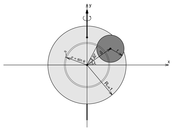
Figure 1: Geometry of the transit illustrating the Rossiter-McLaughling effect.

To compute these momenta, we apply an adaptation of the approach developed by Abubekerov & Gostev (2013) for transit lightcurve modeling. Define auxiliary functions

$$\mathcal{A}(x)=\Re\arccos x=\left\{\begin{array}[]{@{}l@{\;}l@{}}\pi,&x<-1,\\ \arccos x,&|x|<1,\\ 0,&x>1,\end{array}\right.\quad\mathcal{Q}(x)=\Re\sqrt{x}=\left\{\begin{array}[]{@{}l@{\;}l@{}}\sqrt{x},&x>0,\\ 0,&x<0,\end{array}\right.\quad\frac{d\mathcal{A}}{dx}=-\mathcal{Q}\left(\frac{1}{1-x^{2}}\right),\quad\Psi(\delta,x,y)=\mathcal{A}\left(\frac{\delta^{2}+x^{2}-y^{2}}{2x\delta}\right).$$ (4.2)

Then, extending formula (7) from (Abubekerov & Gostev, 2013) to take into account additional factor $x^{k}$, we can write down:

$$M_{k}=\int\limits_{0}^{1}I(\rho)\rho^{k+1}d\rho\int\limits_{-\Psi(\delta,\rho,r)}^{\Psi(\delta,\rho,r)}\cos^{k}(\varphi+\lambda)\,d\varphi.$$ (4.3)

Abubekerov & Gostev (2013) computed $M_{0}$ and its derivatives with respect to $r$ and $\delta$, which are necessary to express the flux reduction $\Delta L$ and its parametric gradient (for further fitting of the model by a gradient descent). Here we also compute $M_{k}$ with their derivatives for $k=1,2,3$.

Let us put $\rho=\sin\theta$. The limb-darkening law is often modelled by a polynomial in $\cos\theta$. Then $M_{k}$ can be expressed via linear combinations of the following integrals

$$H_{nk}=\int\limits_{0}^{\frac{\pi}{2}}\sin^{k+1}\theta\cos^{n+1}\theta\,d\theta\int\limits_{\lambda-\hat{\Psi}}^{\lambda+\hat{\Psi}}\cos^{k}\varphi\,d\varphi,\qquad\hat{\Psi}=\Psi(\delta,\sin\theta,r),\\$$

Assuming at first that $k$ is odd, rewrite $\cos^{k}\varphi$ as a trigonometric sum of multiple argument and compute the inner integral:

$$H_{nk} = \int\limits_{0}^{\frac{\pi}{2}}\sin^{k+1}\theta\cos^{n+1}\theta\,d\theta\int\limits_{\lambda-\hat{\Psi}}^{\lambda+\hat{\Psi}}\frac{1}{2^{k-1}}\sum_{j=0}^{[k/2]}C_{k}^{j}\cos(k-2j)\varphi\,d\varphi=$$ (4.4)

$$= \frac{1}{2^{k-2}}\int\limits_{0}^{\frac{\pi}{2}}\sin^{k+1}\theta\cos^{n+1}\theta\sum_{j=0}^{[k/2]}\frac{C_{k}^{j}}{k-2j}\sin(k-2j)\hat{\Psi}\,\cos(k-2j)\lambda\,d\theta=$$

$$= \frac{1}{2^{k-2}}\sum_{j=0}^{[k/2]}\frac{C_{k}^{j}}{k-2j}\cos(k-2j)\lambda\int\limits_{0}^{\frac{\pi}{2}}\sin^{k+1}\theta\,\cos^{n+1}\theta\,U_{k-2j-1}(\cos\hat{\Psi})\sin\hat{\Psi}\,d\theta.$$

where $U_{n}$ are Chebyshev polynomials of the second kind. If $k$ is even, then the procedure is similar, but the sum should also contain a term with $j=k/2$, which must be handled separately due to a degeneracy. In general, we can represent $H_{nk}$ via the following trigonometric polynomial in $\lambda$:

$$H_{nk}=\sum_{j=0}^{[k/2]}\mathcal{I}_{nkj}\cos(k-2j)\lambda,$$ (4.5)

where

$$\mathcal{I}_{nkj}=\frac{1}{2^{k-2}}\frac{C_{k}^{j}}{k-2j}\int\limits_{0}^{\frac{\pi}{2}}\sin^{k+1}\theta\,\cos^{n+1}\theta\,U_{k-2j-1}(\cos\hat{\Psi})\sin\hat{\Psi}\,d\theta,\quad 2j<k,\qquad\mathcal{I}_{n,2j,j}=\frac{C_{2j}^{j}}{2^{2j-1}}\int\limits_{0}^{\frac{\pi}{2}}\sin^{2j+1}\theta\cos^{n+1}\theta\,\hat{\Psi}\,d\theta.$$ (4.6)

By extracting from $\cos^{n+1}\theta$ a multiplier $\cos^{2}\theta=1-\sin^{2}\theta$, we can obtain the following recurrent relation:

$$\mathcal{I}_{nkj}=\mathcal{I}_{n-2,k,j}-4\frac{(j+1)(k-j+1)}{(k+1)(k+2)}\mathcal{I}_{n-2,k+2,j+1},\qquad 2j\leq k.$$ (4.7)

This can be used to reduce the index $n$ to either $n=0$ or $n=1$, by the cost of increasing $k$ and $j$. In practice we only need this formula to reduce $n=2$ (quadratic limb-darkening term) to $n=0$.

Now let us define

$$a=1-(\delta-r)^{2},\quad a(\theta)=a-\cos^{2}\theta,\qquad b=(\delta+r)^{2}-1,\quad b(\theta)=b+\cos^{2}\theta.$$ (4.8)

This yields

$$\cos\hat{\Psi}\sin\theta=(\delta-r)+\frac{a(\theta)}{2\delta},\qquad\sin\hat{\Psi}\sin\theta=\frac{\mathcal{Q}[a(\theta)b(\theta)]}{2\delta}.$$ (4.9)

In fact, the integration range can be limited to only the range where $\sin\hat{\Psi}\neq 0$, corresponding to $-b\leq\cos^{2}\theta\leq a\leq 1$. For convenience, we need to transform this variable range to a constant one. The case $a<0$ is trivial, as $\sin\hat{\Psi}\equiv 0$ everywhere. In the case $a>0$ we can introduce the following replacement $\theta\mapsto t$:

$$\cos^{2}\theta=a-\min(a,a+b)t^{2},\quad\sin\theta\cos\theta\,d\theta=\min(a,a+b)\,t\,dt.$$ (4.10)

After this replacement, the new integration variable $t$ always spans the same segment $[0,1]$. By making this replacement, expanding Chebyshev polynomials as $U_{n}(x)=\sum_{l=0}^{[n/2]}u_{nl}x^{n-2l}$, and introducing additional auxiliary designations, we may rewrite the integrals $\mathcal{I}_{nkj}$ as follows:

$$\mathcal{I}_{nkj} = \frac{(1-q^{2})^{\frac{n}{2}}}{2^{k-2}}\frac{C_{k}^{j}}{k-2j}\frac{p}{2\delta}\int\limits_{0}^{1}P_{k-j}\left(pt^{2}\right)\sqrt{\max(1,m)-t^{2}}\,\left(1-\min(m,1)t^{2}\right)^{\frac{n}{2}}\,dt,\qquad 2j<k,$$

$$P_{k-j}(x) = x\left(q^{2}+x\right)^{\frac{k-1}{2}}U_{k-2j-1}\left(\frac{q+\frac{x}{2\delta}}{\sqrt{q^{2}+x}}\right)=x\sum_{l=0}^{\left[\frac{k-1}{2}\right]-j}u_{k-2j-1,l}\left(q+\frac{x}{2\delta}\right)^{k-2j-2l-1}\left(q^{2}+x\right)^{j+l}$$ (4.11)

$$q=\delta-r,\qquad m=\frac{4r\delta}{1-q^{2}},\qquad p=\min(4r\delta,1-q^{2})=4r\delta\min\left(1,\frac{1}{m}\right)=(1-q^{2})\min(1,m).$$

Note that although there is a division by $\delta$ in $p/(2\delta)$ and $x/(2\delta)$, in actuality there is no pecularity at $\delta=0$, because by definition $p<4r\delta$ and thus $p/(2\delta)<2r$. Note that $0<m<1$ corresponds to full phase of a transit ($r+\delta<1$), while $m>1$ corresponds to a partial occultation $|r-\delta|<1<r+\delta$. The cases of a full eclipse or no eclipse ($|r-\delta|>1$) would correspond to $m<0$, which are illegal in these formulae by definition. In the latter case, $\mathcal{I}_{nkj}=0$ for $2j<k$.

The case $k=2j$ is more complicated due to a “naked” $\hat{\Psi}$ in the integrad. We may apply two ways of integration by parts:

$$\mathcal{I}_{n,2j,j} = -\frac{C_{2j}^{j}}{2^{2j-1}}\int\limits_{0}^{\frac{\pi}{2}}\hat{\Psi}\sin^{2j}\theta\,\frac{d\cos^{n+2}\theta}{n+2}=\delta_{0j}\frac{2\pi\Theta(-q)}{n+2}+\frac{2j-1}{n+2}\mathcal{I}_{n+2,2j-2,j-1}+\frac{1}{n+2}\frac{C_{2j}^{j}}{2^{2j-1}}\int\limits_{0}^{\frac{\pi}{2}}\sin^{2j}\theta\cos^{n+2}\theta\frac{d\hat{\Psi}}{d\theta}d\theta=$$ (4.12)

$$= \frac{C_{2j}^{j}}{2^{2j-1}}\int\limits_{0}^{\frac{\pi}{2}}\hat{\Psi}\cos^{n}\theta\,\frac{d\sin^{2j+2}\theta}{2j+2}=\delta_{0n}\frac{C_{2j}^{j}}{2^{2j}}\frac{\Psi(\delta,1,r)}{j+1}+\frac{n}{2j+1}\mathcal{I}_{n-2,2j+2,j+1}-\frac{1}{j+1}\frac{C_{2j}^{j}}{2^{2j}}\int\limits_{0}^{\frac{\pi}{2}}\sin^{2j+2}\theta\cos^{n}\theta\frac{d\hat{\Psi}}{d\theta}d\theta,$$

where $\delta_{ik}$ is Kronecker delta (not to be mixed with the planet-star distance $\delta$, which is unindexed), and we use that $\lim_{\rho\to+0}\Psi(\delta,\rho,r)=\pi\Theta(-q)$ (with $\Theta$ being the Heaviside function). Taking into account (4.7), both formulae (4.12) appear to yield the same recurrent relation, if $n\neq 0$:

$$(n+2j+2)\mathcal{I}_{n,2j,j}=(2j-1)\mathcal{I}_{n,2j-2,j-1}+G_{n+2,j},\quad j>0,\qquad G_{nj}=\frac{C_{2j}^{j}}{2^{2j-1}}\int\limits_{0}^{\frac{\pi}{2}}\sin^{2j}\theta\cos^{n}\theta\frac{d\hat{\Psi}}{d\theta}d\theta.$$ (4.13)

For $n=0$ this relation is still valid thanks to the first of eq. (4.12), but we also obtain from the second eq. of (4.12) an independent non-recurrent formula

$$\mathcal{I}_{0,2j,j}=\frac{C_{2j}^{j}}{2^{2j}}\frac{\Psi(\delta,1,r)}{j+1}-\frac{G_{0,j+1}}{2j+1},\quad j\geq 0.$$ (4.14)

It can be verified by direct substitution that this formula satisfies (4.13). The recursion (4.13) can be used to reduce $j$ until we meet $j=0$. For $j=0$ we may use one of the following schemes:

$$(n+2)\mathcal{I}_{n,0,0}=2\pi\Theta(-q)+G_{n+2,0},\qquad\mathcal{I}_{0,0,0}=\Psi(\delta,1,r)-G_{0,1}.$$ (4.15)

We use the second formula of (4.15) for $n=0$, because this simplifies some computations.

To compute $G_{nj}$, we express the derivative of $\hat{\Psi}$ by differentiating $\cos\hat{\Psi}$ and then apply the substitution (4.10):

$$G_{nj}=r(1-q^{2})^{\frac{n}{2}}\frac{C_{2j}^{j}}{2^{2j-2}}\int\limits_{0}^{1}\left(q-\frac{p}{2r}t^{2}\right)\left(q^{2}+pt^{2}\right)^{j-1}\frac{\left(1-\min(1,m)t^{2}\right)^{\frac{n}{2}}}{\sqrt{\max(1,m)-t^{2}}}\,dt.$$ (4.16)

Note that $p/(2r)<2\delta$, so there is no pecularity at $r=0$. Note that in the case of a full eclipse or no eclipse, $|r-\delta|>1$, we have $m<0$ and put $G_{nj}=0$ by definition.

Now let us review the results. Our final useable formulae are (4.5,4.7,4.11,4.13,4.15,4.16). For even $n$ all integrals are elementary, because their integrads are rational functions of $t$ and of the radical $\sqrt{\max(m,1)-t^{2}}$. For odd $n$, the integrands are rational functions of $t$ and $\sqrt{(1-t^{2})(1-\min(m,1/m)t^{2})}$, implying that all integrals are elliptic and can be expressed via Legendre complete elliptic integrals with the parameter $\min(m,1/m)$. In the most cases, this should be only the Legendre integrals of the first and second kind, and only in $G_{1,0}$ we meet the Legendre integral of the third kind, where $t$ is present in a denominator of the integrand’s rational part. This integral, however, affects $\mathcal{I}_{1,2j,j}$ for all $j$, due to the recursion (4.13).

Our approach allows to give exact and explicit formulae for all velocity momenta for any polynomial limb-darkening law. However, in this work we only need momenta up to cubic order ($k=0,1,2,3$) and up to quadratic limb-darkening law ($n=0,1,2$). From now on, we stop using generic notations and focus on the computation of $H_{nk}$ for the specified indices $n$ and $k$.

Consider the quadratic limb-darkening model

$$I(\rho) = I^{\mathrm{c}}(\rho)-\Lambda_{l}I^{\mathrm{l}}(\rho)-\Lambda_{q}I^{\mathrm{q}}(\rho)=(1-\Lambda_{l}-2\Lambda_{q})I^{\mathrm{c}}+(\Lambda_{l}+2\Lambda_{q})(I^{\mathrm{c}}-I^{\mathrm{l}})+\Lambda_{q}(2I^{\mathrm{l}}-I^{\mathrm{q}}),$$ (4.17)

$$I^{\mathrm{c}}=1,\qquad I^{\mathrm{l}}=1-\cos\theta,\quad I^{\mathrm{c}}-I^{\mathrm{l}}=\cos\theta,\qquad I^{\mathrm{q}}=(1-\cos\theta)^{2},\quad 2I^{\mathrm{l}}-I^{\mathrm{q}}=1-\cos^{2}\theta.$$

Therefore, using (4.7) for terms with $n=2$, we have:

$$\begin{array}[]{lll}\lx@intercol M_{k}=(1-\Lambda_{l}-2\Lambda_{q})M_{k}^{\mathrm{c}}+(\Lambda_{l}+2\Lambda_{q})(M_{k}^{\mathrm{c}}-M_{k}^{\mathrm{l}})+\Lambda_{q}(2M_{k}^{\mathrm{l}}-M_{k}^{\mathrm{q}}),\qquad k=0,1,2,3,\hfil\lx@intercol\\ M_{0}^{\mathrm{c}}=\mathcal{I}_{0,0,0},&M_{0}^{\mathrm{c}}-M_{0}^{\mathrm{l}}=\mathcal{I}_{1,0,0},&2M_{0}^{\mathrm{l}}-M_{0}^{\mathrm{q}}=2\mathcal{I}_{0,2,1},\\ M_{1}^{\mathrm{c}}=\mathcal{I}_{0,1,0}\cos\lambda,&M_{1}^{\mathrm{c}}-M_{1}^{\mathrm{l}}=\mathcal{I}_{1,1,0}\cos\lambda,&2M_{1}^{\mathrm{l}}-M_{1}^{\mathrm{q}}=\frac{4}{3}\mathcal{I}_{0,3,1}\cos\lambda,\\ M_{2}^{\mathrm{c}}=\mathcal{I}_{0,2,0}\cos 2\lambda+\mathcal{I}_{0,2,1},&M_{2}^{\mathrm{c}}-M_{2}^{\mathrm{l}}=\mathcal{I}_{1,2,0}\cos 2\lambda+\mathcal{I}_{1,2,1},&2M_{2}^{\mathrm{l}}-M_{2}^{\mathrm{q}}=\mathcal{I}_{0,4,1}\cos 2\lambda+\frac{4}{3}\mathcal{I}_{0,4,2},\\ M_{3}^{\mathrm{c}}=\mathcal{I}_{0,3,0}\cos 3\lambda+\mathcal{I}_{0,3,1}\cos\lambda,&M_{3}^{\mathrm{c}}-M_{3}^{\mathrm{l}}=\mathcal{I}_{1,3,0}\cos 3\lambda+\mathcal{I}_{1,3,1}\cos\lambda,&2M_{2}^{\mathrm{l}}-M_{2}^{\mathrm{q}}=\frac{4}{5}\mathcal{I}_{0,5,1}\cos 3\lambda+\frac{6}{5}\mathcal{I}_{0,5,2}\cos\lambda.\end{array}$$ (4.18)

Thus, we need to compute $16$ integrals $\mathcal{I}_{nkj}$ in total: $11$ of them are of type $k>2j$ (with $7$ elementary, and $4$ elliptic) and $5$ are of type $k=2j$ ($3$ elementary, $2$ elliptic). Note that

$$\mathcal{I}_{0,0,0}=\Psi(\delta,1,r)-G_{0,1},\quad\mathcal{I}_{0,2,1}=\frac{\mathcal{I}_{0,0,0}+G_{2,1}}{4},\quad\mathcal{I}_{0,4,2}=\frac{3\mathcal{I}_{0,2,1}+G_{2,2}}{6},\quad\mathcal{I}_{1,0,0}=\frac{2\pi\Theta(-q)+G_{3,0}}{3},\quad\mathcal{I}_{1,2,1}=\frac{\mathcal{I}_{1,0,0}+G_{3,1}}{5}.$$ (4.19)

The remaining part is to compute integrals (4.11,4.16) for the indices specified above. This is a routine but difficult work due to quickly growing formulae. We used MAPLE computer algebra to compute these integrals in a symbolic form. The results are given in Table 1. We represent all $\mathcal{I}_{nkj}$ and their derivatives as linear combinations of the following functions: elementary $\psi,\varphi$, and $Q$ for $n=0,2$ and elliptic $\tilde{K},\tilde{E}$, and $\tilde{\Pi}$ (or $\tilde{J}$) for $n=1$. The coefficients are algebraic polynomials in $r$ and $\delta$. The degree of these polynomials may reach $8$, and we tried to reduce them by reusing an auxiliary function $W$, whenever possible. All these analytic expressions were verified by comparison with numeric calculation of the integrals.

In this work we adopt the following definition of the complete elliptic integrals (Legendre normal forms):

$$K(m)=\int\limits_{0}^{\frac{\pi}{2}}\frac{d\theta}{\sqrt{1-m\sin^{2}\theta}},\qquad E(m)=\int\limits_{0}^{\frac{\pi}{2}}\sqrt{1-m\sin^{2}\theta}\,d\theta,\qquad\Pi(n|m)=\int\limits_{0}^{\frac{\pi}{2}}\frac{d\theta}{(1+n\sin^{2}\theta)\sqrt{1-m\sin^{2}\theta}}.$$ (4.20)

Note that the sign of $n$ here is opposite to what is adopted by (Abubekerov & Gostev, 2013) and by MAPLE, but it coincides with what is adopted by Carlson (1994) and by the GNU Scientific Library. This choice allows to keep the argument $n$ always positive in our formulae. To compute these integrals we recommend the algorithms by Fukushima (2013). This method appears faster by the factor of a few in comparison with the Carlson (1994) symmetric forms approach, which was selected by Abubekerov & Gostev (2013) and also adopted in the GNU Scientific Library. Fukushima (2013) uses the following “associated” forms of elliptic integrals (note that we also changed sign of $n$ here):

$$B(m)=\int\limits_{0}^{\frac{\pi}{2}}\frac{\cos^{2}\theta\,d\theta}{\sqrt{1-m\sin^{2}\theta}},\qquad D(m)=\int\limits_{0}^{\frac{\pi}{2}}\frac{\sin^{2}\theta\,d\theta}{\sqrt{1-m\sin^{2}\theta}},\qquad J(n|m)=\int\limits_{0}^{\frac{\pi}{2}}\frac{\sin^{2}\theta\,d\theta}{(1+n\sin^{2}\theta)\sqrt{1-m\sin^{2}\theta}}.$$ (4.21)

This implies:

$$K(m)=B(m)+D(m),\quad E(m)=B(m)+(1-m)D(m),\quad\Pi(n|m)=K(m)-nJ(n|m).$$ (4.22)

Additionally, the following identity from (Fukushima, 2013) becomes useful for us:

$$J(n|m)=-\frac{\pi}{2}\frac{1}{\sqrt{n(1+n)(n+m)}}+\frac{1}{n}K(m)-\frac{m}{n^{2}}J\left(\frac{m}{n}\Big{|}m\right).$$ (4.23)

This identity was used to remove an undesired discontinuity near $\delta=r$ that appeared in the original MAPLE output, which was expressed via $\Pi$ (see intermediary quantity $\Omega$ in Table 1).

Some formulae in Table 1 contain an apparent pecularity near $\delta=0$ due to division by $\delta$. All functions are actually smooth at $\delta=0$, but the pecularity is associated with the subtraction of close number like $K(\epsilon)-E(\epsilon)$ for $\epsilon\approx 0$. This leads to an accuracy loss near $\delta=0$. To get rid of it, we might rewrite the formulae using some non-standard elliptic functions as a basis, but this is not convenient, so we choose to consider the case $\delta\approx 0$ separately and provide in Table 2 the relevant Taylor series about $\delta=0$. These series are more preferred than general formulae, if $\delta<0.05(1-r^{2})$. We give these series only for elliptic integrals $n=1$ and only for the case of the full phase of a transit, $r+\delta<1$. The case of a partial occultation is possible with small $\delta$ only if an additional condition $r\approx 1$ is satisfied. In practice it is a rare condition when simultaneously $\delta$ is small and $r$ is close to unit (a close-to-ring eclipse). Besides, numerical tests did not reveal significant loss of precision in this parametric domain.

Note that our results for $M_{0}$ (which is responsible only for the flux decrease) are in agreement with Abubekerov & Gostev (2013). Also, substituting $\delta=0$ and $r=1$ in $M_{k}$ we obtain values for the whole-disk momenta $M_{k}^{\star}$:

$$M_{0}^{\star}=\pi-\frac{\pi}{3}\Lambda_{l}-\frac{\pi}{6}\Lambda_{q},\qquad M_{2}^{\star}=\frac{\pi}{4}-\frac{7\pi}{60}\Lambda_{l}-\frac{\pi}{15}\Lambda_{q},\qquad M_{1,3}^{\star}=0.$$ (4.24)

In addition to the expressions (4.18) we may also need to compute partial derivatives of $M_{k}$ with respect to $\lambda$, which are trivial, or with respect to the planet coordinates $x,y$ in the projection plane. We can use the following formulae for this goal:

$$\delta^{2}=x^{2}+y^{2},\quad\frac{\partial\delta}{\partial x}=\frac{x}{\delta},\quad\frac{\partial\delta}{\partial y}=\frac{y}{\delta},\quad\cos n\lambda=T_{n}\left(\frac{x}{\delta}\right),\quad\frac{\partial\cos n\lambda}{\partial x}=n\frac{y^{2}}{\delta^{3}}U_{n-1}\left(\frac{x}{\delta}\right),\quad\frac{\partial\cos n\lambda}{\partial y}=-n\frac{xy}{\delta^{3}}U_{n-1}\left(\frac{x}{\delta}\right).$$ (4.25)

Here $T_{n}$ and $U_{n}$ are Chebyshev polynomials of the first and second kind.

Table 1: Integrals $\mathcal{I}_{nkj}(\delta,r)$ and their derivatives: general formulae.

Function $f$	$f(\delta,r)$	$\partial f/\partial r$	$\partial f/\partial\delta$
$\mathcal{I}_{000}$	$\psi+r^{2}\varphi-\frac{Q}{2}$	$2r\varphi$	$-\frac{Q}{\delta}$
$\mathcal{I}_{010}$	$r^{2}\delta\varphi+(1-\delta^{2}-r^{2})\frac{Q}{4\delta}$	$2r\delta\varphi-\frac{rQ}{\delta}$	$r^{2}\varphi+(r^{2}-3\delta^{2}-1)\frac{Q}{4\delta^{2}}$
$\mathcal{I}_{020}$	$r^{2}\delta^{2}\frac{\varphi}{2}+\left[3\delta^{2}(1-r^{2}-\delta^{2})-W\right]\frac{Q}{24\delta^{2}}$	$r\delta^{2}\varphi+(r^{2}-3\delta^{2}-1)\frac{rQ}{4\delta^{2}}$	$r^{2}\delta\varphi+\left[W-3\delta^{2}(r^{2}+\delta^{2}+1)\right]\frac{Q}{12\delta^{3}}$
$\mathcal{I}_{030}$	$\begin{aligned} r^{2}\delta^{3}\frac{\varphi}{4}+&\left[6\delta^{2}(r^{4}-3r^{2}\delta^{2}-2r^{2}-\delta^{2}+1)-\right.\\ &\left.-(1-r^{2}-3\delta^{2})W\right]\frac{Q}{96\delta^{3}}\end{aligned}$	$r\delta^{3}\frac{\varphi}{2}+\left[2W+3\delta^{2}(r^{2}-3\delta^{2}-3)\right]\frac{rQ}{24\delta^{3}}$	$\begin{aligned} r^{2}\delta^{2}\frac{3\varphi}{4}+&\left[2\delta^{2}(3r^{4}-9r^{2}\delta^{2}-4r^{2}-5\delta^{2}+1)+\right.\\ &\left.+(1-r^{2}+5\delta^{2})W\right]\frac{Q}{32\delta^{4}}\end{aligned}$
$\mathcal{I}_{021}$	$\frac{\psi}{4}+r^{2}(r^{2}+2\delta^{2})\frac{\varphi}{4}-(5r^{2}+\delta^{2}+1)\frac{Q}{16}$	$r(r^{2}+\delta^{2})\varphi-rQ$	$r^{2}\delta\varphi-(r^{2}+\delta^{2}+1)\frac{Q}{4\delta}$
$\mathcal{I}_{031}$	$r^{2}\delta(r^{2}+\delta^{2})\frac{3\varphi}{4}+\left[3(r^{2}+\delta^{2})(1-r^{2}-\delta^{2})-2W\right]\frac{Q}{16\delta}$	$r\delta(2r^{2}+\delta^{2})\frac{3\varphi}{2}-(1+r^{2}+5\delta^{2})\frac{3rQ}{8\delta}$	$r^{2}(r^{2}+3\delta^{2})\frac{3\varphi}{4}+(r^{4}-5\delta^{4}-20r^{2}\delta^{2}+r^{2}-5\delta^{2}-2)\frac{Q}{16\delta^{2}}$
$\mathcal{I}_{041}$	$\begin{aligned} r^{2}\delta^{2}(3r^{2}+2\delta^{2})\frac{\varphi}{4}-\left[(r^{2}-3\delta^{2}+3)W+\right.\\ \left.+6\delta^{2}(r^{4}+9r^{2}\delta^{2}+2\delta^{2}+r^{2}-2)\right]\frac{Q}{96\delta^{2}}\end{aligned}$	$\begin{aligned} &r\delta^{2}(3r^{2}+\delta^{2})\varphi+\\ &+(r^{4}-17\delta^{4}-8r^{2}\delta^{2}+r^{2}-5\delta^{2}-2)\frac{rQ}{12\delta^{2}}\end{aligned}$	$\begin{aligned} r^{2}\delta(3r^{2}+4\delta^{2})\frac{\varphi}{2}+\left[(r^{2}+9\delta^{2}+3)W+\right.\\ \left.+6\delta^{2}(r^{4}-15r^{2}\delta^{2}-5r^{2}-4\delta^{2})\right]\frac{Q}{48\delta^{3}}\end{aligned}$
$\mathcal{I}_{051}$	$\begin{aligned} &r^{2}\delta^{3}(2r^{2}+\delta^{2})\frac{5\varphi}{16}+\left[30\delta^{4}(2r^{2}+\delta^{2})(1-r^{2}-\delta^{2})-\right.\\ &\left.-(1+5\delta^{4}+2\delta^{2}-r^{2}+r^{2}\delta^{2})5W-W^{2}\right]\frac{Q}{384\delta^{3}}\end{aligned}$	$\begin{aligned} &r\delta^{3}(4r^{2}+\delta^{2})\frac{5\varphi}{8}+\left[(3+r^{2}+37\delta^{2})W+\right.\\ &\left.+6\delta^{2}(7r^{4}-17r^{2}\delta^{2}-13r^{2}-14\delta^{2}+4)\right]\frac{5rQ}{192\delta^{3}}\end{aligned}$	$\begin{aligned} r^{2}\delta^{2}(6r^{2}+5\delta^{2})\frac{5\varphi}{16}-\left[(r^{2}\delta^{2}-9\delta^{4}+3r^{2}-24\delta^{2}-3)5W-3W^{2}+\right.\\ \left.+30\delta^{2}(r^{4}\delta^{2}+21r^{2}\delta^{4}-5r^{4}+14r^{2}\delta^{2}+8r^{2}+7\delta^{2}-3)\right]\frac{Q}{384\delta^{4}}\end{aligned}$
$\mathcal{I}_{042}$	$\begin{aligned} &\frac{\psi}{8}+r^{2}(r^{4}+6r^{2}\delta^{2}+3\delta^{4})\frac{\varphi}{8}-\\ &-(10r^{4}+\delta^{4}+19r^{2}\delta^{2}+4r^{2}+\delta^{2}+1)\frac{Q}{48}\end{aligned}$	$r(r^{4}+4r^{2}\delta^{2}+\delta^{4})\frac{3\varphi}{4}-(1+3r^{2}+3\delta^{2})\frac{3rQ}{8}$	$r^{2}\delta(r^{2}+\delta^{2})\frac{3\varphi}{2}+\left[W-3(4r^{2}\delta^{2}+r^{2}+\delta^{2})\right]\frac{Q}{8\delta}$
$\mathcal{I}_{052}$	$\begin{aligned} r^{2}\delta&(r^{4}+3r^{2}\delta^{2}+\delta^{4})\frac{5\varphi}{8}+\left[(3+r^{2}+\delta^{2})W-\right.\\ &\left.-6(5r^{2}\delta^{4}+5r^{4}\delta^{2}+3r^{2}\delta^{2}+r^{2}+\delta^{2}-1)\right]\frac{5Q}{192\delta}\end{aligned}$	$\begin{aligned} r\delta&(3r^{4}+6r^{2}\delta^{2}+\delta^{4})\frac{5\varphi}{4}+\\ &+\left[W-3(7r^{2}\delta^{2}+3\delta^{4}+r^{2}+2\delta^{2})\right]\frac{5rQ}{24\delta}\end{aligned}$	$\begin{aligned} r^{2}&(r^{4}+9r^{2}\delta^{2}+5\delta^{4})\frac{5\varphi}{8}-\left[(r^{2}-7\delta^{2}+3)W+\right.\\ &\left.+6(7r^{4}\delta^{2}+23r^{2}\delta^{4}+5r^{2}\delta^{2}+4\delta^{4}-r^{2}-\delta^{2}+1)\right]\frac{5Q}{192\delta^{2}}\end{aligned}$
$\mathcal{I}_{100}$	$\frac{2}{3}\Omega+\frac{2}{9}\left[(7r^{2}+\delta^{2}-4)\tilde{E}-W\tilde{K}\right]$	$4r\tilde{E}$	$\frac{2}{3\delta}\left[(r^{2}+\delta^{2}-1)\tilde{E}-W\tilde{K}\right]$
$\mathcal{I}_{110}$	$\frac{2}{15\delta}\left[(16r^{2}\delta^{2}-W)\tilde{E}+(1-\delta^{2}-r^{2})W\tilde{K}\right]$	$\frac{2r}{3\delta}\left[(r^{2}+7\delta^{2}-1)\tilde{E}-W\tilde{K}\right]$	$\frac{2}{15\delta^{2}}\left\{(r^{2}-4\delta^{2}-1)W\tilde{K}+\left[\delta^{2}(19r^{2}+5\delta^{2}-5)+W\right]\tilde{E}\right\}$
$\mathcal{I}_{120}$	$\begin{aligned} &\frac{1}{105\delta^{2}}\left\{-\left[\delta^{2}(9r^{2}+7\delta^{2}-7)+2W\right]W\tilde{K}+\right.\\ &\left.+\left[8r^{2}\delta^{2}(r^{2}+15\delta^{2}-1)+(2r^{2}-5\delta^{2}-2)W\right]\tilde{E}\right\}\end{aligned}$	$\begin{aligned} \frac{2r}{15\delta^{2}}&\left\{(r^{2}-4\delta^{2}-1)W\tilde{K}+\right.\\ &\left.+\left[\delta^{2}(4r^{2}+20\delta^{2}-5)+W\right]\tilde{E}\right\}\end{aligned}$	$\begin{aligned} \frac{1}{105\delta^{3}}&\left\{\left[4W-\delta^{2}(17r^{2}+21\delta^{2}+14)\right]W\tilde{K}-\left[(4r^{2}+25\delta^{2}-4)W+\right.\right.\\ &\left.\left.+\delta^{2}(16r^{4}-35\delta^{2}-320r^{2}\delta^{2}-51r^{2}+35)\right]\tilde{E}\right\}\end{aligned}$
$\mathcal{I}_{130}$	$\begin{aligned} &\frac{1}{1890\delta^{3}}\left\{-\left[\delta^{2}(224r^{2}\delta^{2}+63\delta^{2}-64r^{4}+127r^{2}-63)+\right.\right.\\ &\left.\left.+(8-8r^{2}-35\delta^{2})W\right]W\tilde{K}+\left[16r^{2}\delta^{4}(8r^{2}+72\delta^{2}-9)+\right.\right.\\ &\left.\left.+\delta^{2}(29r^{2}-27\delta^{2}-36)W+8W^{2}\right]\tilde{E}\right\}\end{aligned}$	$\begin{aligned} &\frac{r}{210\delta^{3}}\left\{\left[3\delta^{2}(5r^{2}-21\delta^{2}-14)+8W\right]W\tilde{K}-\right.\\ &\left.-\left[3\delta^{2}(104r^{4}-232r^{2}\delta^{2}-175\delta^{2}-209r^{2}+105)+\right.\right.\\ &\left.\left.\phantom{-\big{[}}+(8r^{2}+281\delta^{2}-8)W\right]\tilde{E}\right\}\end{aligned}$	$\begin{aligned} &\frac{1}{630\delta^{4}}\left\{\left[\delta^{4}(40r^{4}+1368r^{2}\delta^{2}+39r^{2}-105+105\delta^{2})+\right.\right.\\ &\left.\left.+\delta^{2}(13r^{2}-78\delta^{2}+36)W-8W^{2}\right]\tilde{E}+\left[(8-8r^{2}+70\delta^{2})W+\right.\right.\\ &\left.\left.+\delta^{2}(83r^{4}-259r^{2}\delta^{2}-125r^{2}-147\delta^{2}+42)\right]W\tilde{K}\right\}\end{aligned}$
$\mathcal{I}_{121}$	$\begin{aligned} &\frac{2}{15}\Omega-\frac{1}{225}\left[(39r^{2}+9\delta^{2}+1)W\tilde{K}-\right.\\ &\left.-(129r^{4}+9\delta^{4}-68r^{2}+246r^{2}\delta^{2}-8\delta^{2}-31)\tilde{E}\right]\end{aligned}$	$\frac{2r}{3}\left[(4r^{2}+4\delta^{2}-1)\tilde{E}-W\tilde{K}\right]$	$\frac{1}{15\delta}\left[(48r^{2}\delta^{2}+5r^{2}+5\delta^{2}-5-3W)\tilde{E}-(3r^{2}+3\delta^{2}+2)W\tilde{K}\right]$
$\mathcal{I}_{131}$	$\begin{aligned} &-\frac{1}{70\delta}\left\{(32r^{2}\delta^{2}+7r^{2}+7\delta^{2}-7-3W)W\tilde{K}+\right.\\ &\left.+\left[16r^{2}\delta^{2}(1-8r^{2}-8\delta^{2})+(4+3r^{2}+3\delta^{2})W\right]\tilde{E}\right\}\end{aligned}$	$\begin{aligned} \frac{r}{10\delta}&\left[(88r^{2}\delta^{2}+40\delta^{4}+5r^{2}-5\delta^{2}-5-3W)\tilde{E}-\right.\\ &\left.-(3r^{2}+13\delta^{2}+2)W\tilde{K}\right]\end{aligned}$	$\begin{aligned} &\frac{1}{70\delta^{2}}\left\{-(59r^{2}\delta^{2}+21\delta^{4}-7r^{2}+7\delta^{2}+7+3W)W\tilde{K}+\right.\\ &\left.+\left[\delta^{2}(152r^{4}+488r^{2}\delta^{2}-19r^{2}+35\delta^{2}-35)+(4+3r^{2}-18\delta^{2})W\right]\tilde{E}\right\}\end{aligned}$
Auxiliary	$\psi=\Psi(\delta,1,r)\in\left[0,\pi\right],\quad\varphi=\Psi(\delta,r,1)\in\left[0,\pi\right],\qquad a=1-(\delta-r)^{2},\quad b=(\delta+r)^{2}-1,\quad W=ab,\qquad Q=\mathcal{Q}[W],\quad Q\text{ nonzero only if }r+\delta>1\text{ and }|r-\delta|<1;$
	$\tilde{K}=K\left(\frac{4r\delta}{a}\right)\big{/}\sqrt{a},\qquad\tilde{E}=\sqrt{a}\,E\left(\frac{4r\delta}{a}\right),\qquad\qquad\tilde{\Pi}=\Pi\left(\frac{4r\delta}{(\delta-r)^{2}},\frac{4r\delta}{a}\right)\big{/}\sqrt{a},\qquad\tilde{J}=a^{-3/2}J\left(\frac{(\delta-r)^{2}}{a},\frac{4r\delta}{a}\right)-\tilde{K}\qquad\quad\mathrm{if}\;r+\delta<1\;(\text{implies }|r-\delta|<1);$
	$\tilde{K}=K\left(\frac{a}{4r\delta}\right)\big{/}\sqrt{4r\delta},\qquad\tilde{E}=\sqrt{4r\delta}\,E\left(\frac{a}{4r\delta}\right)-b\tilde{K},\qquad\tilde{\Pi}=\Pi\left(\frac{a}{(\delta-r)^{2}},\frac{a}{4r\delta}\right)\big{/}\sqrt{4r\delta},\qquad\tilde{J}=(4r\delta)^{-3/2}J\left(\frac{(\delta-r)^{2}}{4r\delta},\frac{a}{4r\delta}\right)-\tilde{K}\qquad\mathrm{if}\;r+\delta>1\text{ and }|r-\delta|<1;$
	$\tilde{K}=\tilde{E}=\tilde{\Pi}=0\qquad\mathrm{if}\;|r-\delta|>1\;(\text{implies }r+\delta>1);\qquad\Omega(\delta,r)=\pi\Theta(r-\delta)+\frac{\delta+r}{\delta-r}\tilde{\Pi}+(r^{2}-\delta^{2})\tilde{K}=\frac{\pi}{2}+(\delta^{2}-r^{2})\tilde{J}\quad(\text{see text for proof}).$

Table 2: Integrals $\mathcal{I}_{nkj}$ and their derivatives near $\delta=0$.

function $f$	$f(\delta,r)$	$\frac{\partial f}{\partial r}$	$\frac{\partial f}{\partial\delta}$
$\mathcal{I}_{100}$	$\frac{2\pi}{3}\left[1-(1-r^{2})^{3/2}\right]-\frac{\pi r^{2}\delta^{2}}{2\sqrt{1-r^{2}}}\left[1+\frac{4-r^{2}}{(1-r^{2})^{2}}\frac{\delta^{2}}{16}\right]+\mathcal{O}(\delta^{6})$	$2\pi r\sqrt{1-r^{2}}\left[1+\frac{r^{2}-2}{(1-r^{2})^{2}}\frac{\delta^{2}}{4}+\frac{r^{4}-8r^{2}-8}{(1-r^{2})^{4}}\frac{\delta^{4}}{64}\right]+\mathcal{O}(\delta^{6})$	$-\frac{\pi r^{2}\delta}{\sqrt{1-r^{2}}}\left[1+\frac{4-r^{2}}{(1-r^{2})^{2}}\frac{\delta^{2}}{8}\right]+\mathcal{O}(\delta^{5})$
$\mathcal{I}_{110}$	$\pi r^{2}\delta\sqrt{1-r^{2}}\left[1+\frac{3r^{2}-4}{(1-r^{2})^{2}}\frac{\delta^{2}}{8}-\frac{r^{4}-4r^{2}+8}{(1-r^{2})^{4}}\frac{\delta^{4}}{64}\right]+\mathcal{O}(\delta^{7})$	$\begin{aligned} \frac{2\pi r\delta}{\sqrt{1-r^{2}}}&\left[1-\frac{3}{2}r^{2}-\frac{3r^{4}-8r^{2}+8}{(1-r^{2})^{2}}\frac{\delta^{2}}{16}-\right.\\ &-\left.\frac{r^{6}-6r^{4}+24r^{2}+16}{(1-r^{2})^{4}}\frac{\delta^{4}}{128}\right]+\mathcal{O}(\delta^{7})\end{aligned}$	$\begin{aligned} \pi r^{2}\sqrt{1-r^{2}}&\left[1+\frac{3r^{2}-4}{(1-r^{2})^{2}}\frac{3\delta^{2}}{8}-\right.\\ &\left.-\frac{r^{4}-4r^{2}+8}{(1-r^{2})^{4}}\frac{5\delta^{4}}{64}\right]+\mathcal{O}(\delta^{6})\end{aligned}$
$\mathcal{I}_{120}$	$\frac{\pi r^{2}\delta^{2}}{2\sqrt{1-r^{2}}}\left[1-\frac{5}{4}r^{2}-\frac{5r^{4}-12r^{2}+8}{(1-r^{2})^{2}}\frac{\delta^{2}}{16}\right]+\mathcal{O}(\delta^{6})$	$\begin{aligned} \frac{\pi r\delta^{2}}{(1-r^{2})^{3/2}}&\left[1-3r^{2}+\frac{15}{8}r^{4}+\right.\\ &\left.+\frac{5r^{6}-18r^{4}+24r^{2}-16}{(1-r^{2})^{2}}\frac{\delta^{2}}{32}\right]+\mathcal{O}(\delta^{6})\end{aligned}$	$\frac{\pi r^{2}\delta}{\sqrt{1-r^{2}}}\left[1-\frac{5}{4}r^{2}-\frac{5r^{4}-12r^{2}+8}{(1-r^{2})^{2}}\frac{\delta^{2}}{8}\right]+\mathcal{O}(\delta^{5})$
$\mathcal{I}_{130}$	$\begin{aligned} \frac{\pi r^{2}\delta^{3}}{4(1-r^{2})^{3/2}}&\left[\vphantom{\frac{r^{6}}{(1-r^{2})^{2}}}1-\frac{5}{2}r^{2}+\frac{35}{24}r^{4}+\right.\\ &\left.+\frac{35r^{6}-120r^{4}+144r^{2}-64}{(1-r^{2})^{2}}\frac{\delta^{2}}{128}\right]+\mathcal{O}(\delta^{7})\end{aligned}$	$\begin{aligned} &\frac{\pi r\delta^{3}}{2(1-r^{2})^{5/2}}\left[\vphantom{\frac{r^{8}}{(1-r^{2})^{2}}}1-\frac{9}{2}r^{2}+\frac{45}{8}r^{4}-\frac{35}{16}r^{6}-\right.\\ &\left.\phantom{ww}-\frac{35r^{8}-160r^{6}+288r^{4}-256r^{2}+128}{(1-r^{2})^{2}}\frac{\delta^{2}}{256}\right]+\mathcal{O}(\delta^{7})\end{aligned}$	$\begin{aligned} \frac{3\pi r^{2}\delta^{2}}{4(1-r^{2})^{3/2}}&\left[\vphantom{\frac{r^{6}}{(1-r^{2})^{2}}}1-\frac{5}{2}r^{2}+\frac{35}{24}r^{4}+\right.\\ &\left.+\frac{35r^{6}-120r^{4}+144r^{2}-64}{(1-r^{2})^{2}}\frac{5\delta^{2}}{384}\right]+\mathcal{O}(\delta^{6})\end{aligned}$
$\mathcal{I}_{121}$	$\begin{aligned} \frac{2\pi}{15}&\left[1-\left(1+\frac{3}{2}r^{2}\right)(1-r^{2})^{3/2}\right]+\\ &+\frac{\pi r^{2}\delta^{2}}{2\sqrt{1-r^{2}}}\left[1-\frac{3}{2}r^{2}-\frac{9r^{4}-22r^{2}+16}{(1-r^{2})^{2}}\frac{\delta^{2}}{32}\right]+\mathcal{O}(\delta^{6})\end{aligned}$	$\begin{aligned} \pi r\sqrt{1-r^{2}}&\left[r^{2}+\frac{9r^{4}-14r^{2}+4}{(1-r^{2})^{2}}\frac{\delta^{2}}{4}+\right.\\ &\left.+\frac{9r^{6}-32r^{4}+40r^{2}-32}{(1-r^{2})^{4}}\frac{\delta^{4}}{64}\right]+\mathcal{O}(\delta^{6})\end{aligned}$	$\frac{\pi r^{2}\delta}{\sqrt{1-r^{2}}}\left[1-\frac{3}{2}r^{2}-\frac{9r^{4}-22r^{2}+16}{(1-r^{2})^{2}}\frac{\delta^{2}}{16}\right]+\mathcal{O}(\delta^{5})$
$\mathcal{I}_{131}$	$\begin{aligned} \frac{3\pi}{4}r^{2}\delta\sqrt{1-r^{2}}&\left[r^{2}+\frac{15r^{4}-24r^{2}+8}{(1-r^{2})^{2}}\frac{\delta^{2}}{8}+\right.\\ &\left.+\frac{15r^{6}-52r^{4}+64r^{2}-32}{(1-r^{2})^{4}}\frac{\delta^{4}}{64}\right]+\mathcal{O}(\delta^{7})\end{aligned}$	$\begin{aligned} \frac{3\pi r\delta}{\sqrt{1-r^{2}}}&\left[r^{2}-\frac{5}{4}r^{4}-\frac{45r^{6}-114r^{4}+88r^{2}-16}{(1-r^{2})^{2}}\frac{\delta^{2}}{32}-\right.\\ &\left.-\frac{15r^{8}-68r^{6}+120r^{4}-96r^{2}+64}{(1-r^{2})^{4}}\frac{\delta^{4}}{256}\right]+\mathcal{O}(\delta^{7})\end{aligned}$	$\begin{aligned} \frac{3\pi}{4}r^{2}\sqrt{1-r^{2}}&\left[r^{2}+\frac{15r^{4}-24r^{2}+8}{(1-r^{2})^{2}}\frac{3\delta^{2}}{8}+\right.\\ &\left.+\frac{15r^{6}-52r^{4}+64r^{2}-32}{(1-r^{2})^{4}}\frac{5\delta^{4}}{64}\right]+\mathcal{O}(\delta^{6})\end{aligned}$
	Assuming that $r+\delta<1$ (full phase of a transit) that implies $r,\delta<1$ and $|r-\delta|<1$.

5 Investigating model applicability by numerical tests

As far as our model employs power-series decompositions in $\upsilon$, it should be applicable only if $\upsilon$ is below some limit. However, such a limit is difficult to predict theoretically. To determine the actual domain of the applicability, we use numerical simulations.

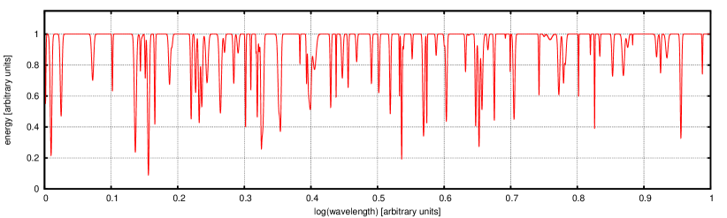
Figure 2: Synthetic star surface spectrum used in the test simulation (Sect. 5). The spectrum contains $100$ Gaussian lines with random characteristics.

First of all, we construct a simulated spectrum $\mathcal{F}$ containing only Gaussian lines with randomly chosen characteristics (Fig. 2). This spectrum we use to perform direct numerical integrations in (2.1). We compute the out-of-transit spectrum $\mathcal{F}_{\star}$ on a grid of $\upsilon$, and the in-transit ones $\mathcal{F}_{\mathrm{p}}$ on a $4$-dimensional grid of the parameters $\upsilon,r,\delta,\lambda$. After that, we fit numerically each in-transit spectrum $\mathcal{F}_{\mathrm{t}}=\mathcal{F}_{\star}-\mathcal{F}_{\mathrm{p}}$ with a shifted $\mathcal{F}_{\star}$, determining the best fitting shift. In such a way, we obtain a set of simulated Doppler shifts as a table function of the gridded values $(\upsilon,r,\delta,\lambda)$. Simultaneously, we compute our analytic RM model (3.4) on the same grid, and then compare the results.

However, it is very difficult to seize a four-dimensional space, so we need to convolve some of the dimensions somehow. We consider $\upsilon$ as our primary parameter of interest, and for each selected $\upsilon$ we compute only r.m.s. of the RM model residuals, corresponding to $(r,\delta,\lambda)$ from the grid. The domain of the grid was constructed as follows: $r\in[0.05,1.22]$, $\delta\in[\max(r-1,0),1+r]$, $\lambda\in[0,\pi]$. The values of $\upsilon$ were ranged approximately from $1/3$ to $10$ times the average line width. A subtle but important detail in this algorithm is that different $r$ imply different amplitudes of the RM curve, scaling roughly as $r^{2}$. Therefore, we introduced an additional descaling factor of $\propto 1/r^{2}$ to equibalance the contribution of different curves in the cumulative r.m.s.

To compute the RM model (3.4), we apply three distinct methods to determine the coefficients $\nu$ and $\mu$. In the first case, we derive them from the original spectrum $\mathcal{F}$, which in practice would not be accessible to the observer. In the second case, we derive $\nu$ and $\mu$ from the observable spectrum $\mathcal{F}_{\star}$. And finally, in the third method we just fit our simulated RM curves with (3.4), assuming that $\upsilon$, $\nu$, and $\mu$ are all free regression coefficients. As we discussed above, the first two methods are equivalent for small $\upsilon$, whenever only the three decomposition terms (3.4) are significant. But for larger $\upsilon$ more terms enter in the game, making it important, which of the spectra was in use for $\nu$ and $\mu$. The third method is the one that can be most easily implemented in practice, if the original spectra are not available at all.

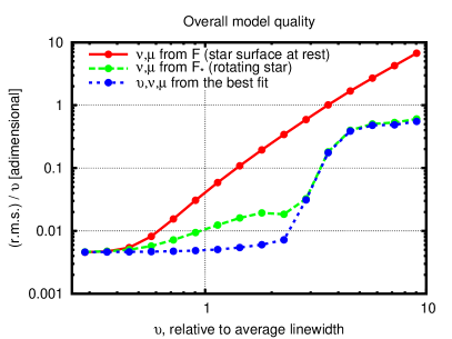
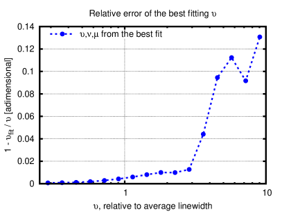
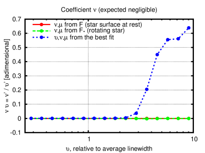
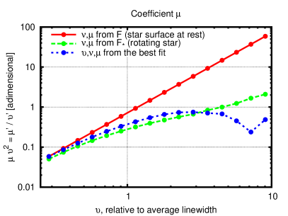
Figure 3: Results of the test simulation from Sect. 5. The abscissa is the value of $\upsilon$ normalized by the average linewidth for lines in the original spectrum $\mathcal{F}$ (not the rotation-broadened $\mathcal{F}_{\star}$). The ordinate in the first plot is a normalized value (r.m.s.)/$\upsilon$. The value of r.m.s. also contains an internal normalization by $1/r^{2}$ (see text), so the graph virtually shows an average relative error of the model (i.e., residuals are normalized by the amplitudes of the relevant RM curves). In the last two plots we show adimensional quantities $\nu\upsilon$ and $\mu\upsilon^{2}$, which reflect the relative contribution of the corresponding correction terms in the model (3.4). See text for details and discussion.

Our main results of the simulation are demonstrated in Fig. 3. In this figure, we have four plots that show how the following quantities depend on $\upsilon$: (i) normalized r.m.s., (ii) relative bias of the best fitting $\upsilon$, (iii) predicted and best fitting values of $\nu$ (all must be negligible in our model), (iv) predicted and best fitting values of $\mu$. From these plots, we can draw the following main conclusions:

1. It is much better to use $\mathcal{F}_{\star}$ for computation of the coefficients $\nu$ and $\mu$, while using $\mathcal{F}$ infers larger errors. It is very favourable to us, because the spectrum that we obtain from observations is also $\mathcal{F}_{\star}$, and not $\mathcal{F}$.

2. If we use $\mathcal{F}$ to compute $\nu$ and $\mu$, the maximum value of the rotation velocity, after which our model becomes inacceptable, is only about the average linewidth (for the lines in the original spectrum $\mathcal{F}$). If we use $\mathcal{F}_{\star}$ to compute $\nu$ and $\mu$, this limit increases to $2-3$ times the average linewidth.

3. The best fitting values of $\nu$ and $\mu$ are close to those derived from $\mathcal{F}_{\star}$.

In the summary we may note, that the range of applicability for our model appears rather optimistic. Even though we used spectra decompositions into powers of $\upsilon$, our model remains accurate even if $\upsilon$ exceeds the average linewidth. In fact, it is more adequate to say that our model requires that “$\upsilon$ is not so large” instead of “$\upsilon$ is small”.

6 Practical application: the case of HD 189733

As the number of formulae appearing above was large, let us now describe a concise step-by-step scheme to compute the RM anomaly:

1. Compute $\mathcal{I}_{nkj}$ based on formulae from Table 1 or 2, if $\delta<0.05(1-r^{2})$. Depending on the expected degree of RM anomaly approximation ($1,2$, or $3$) and degree of the limb-darkening model ($0,1$, or $2$), not all of these $16$ integrals may be actually needed. Whenever the RM anomaly curve is not plainly modelled but also fitted based on the RV data, also compute partial derivatives of $\mathcal{I}_{nkj}$ to be used in the gradient minimization of the chi-square or other goodness-of-fit function.

2. Compute momenta $M_{k}$ from (4.18). Again, not all of them may be necessary, depending on the particular practical task. If needed for further fitting of the anomaly, simultaneously compute the derivatives of $M_{k}$ with respect to $x,y$, and $r$, based on eq. (4.25).

3. Use formulae (3.4) or (3.10) to finally compute the RM anomaly. If necessary, the gradient of the model with respect to the parameters can be obtained based on (3.5) and on partial derivatives from the previous steps. The coefficients near $V_{1,2,3}$ can all be treated as free parameters of the fit.

During the transit, the quantities $\delta$ and $\lambda$ are varying along the projected planet trajectory. This algorithm is not responsible for modelling the planetary orbital motion during the transit, which must be carried out separately, e.g. based on a Keplerian or $N$-body model. We omit a consideration of such models in our paper, as this topic is already investigated quite well.

We do not take into account the effect of finite light speed that may cause a subtle time delay between the RV variation due to the planetary orbitaly motion and the RM anomaly. This delay appears because the former RV shift is imprinted when the light is emitted from the stellar surface, while the latter one appears when the light is blocked but the transiting planet, which occurs closer to the observer. This delay should be usually small, e.g. $\sim 10-20$ sec for a typical hot Jupiter. This effect is not very hard to model, but this falls out of the scope of the present paper, so we neglect it.

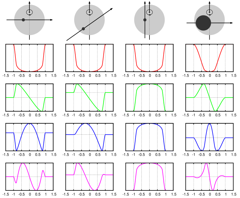
Figure 4: Light curves ($1-f$) for several sample transit configurations shown on top, and plots of the RM anomaly terms $V_{1}$, $V_{2}$, and $V_{3}$ exposed in successive rows downwards. In each graph, the abscissa is a normalized time with first contact at $-1$ and fourth contact at $+1$. The scale and labels of the ordinates are omitted, because we intend to demonstrate only shapes of the curves here. The plots assume the limb darkening with $\Lambda_{l}=\Lambda_{q}=0.25$.

First of all, let us gain some impression of the behaviour of the basis functions $V_{1,2,3}$. During the transit, they can be viewed as functions of the time, and they also depend on the transit geometry. We plot them in Fig. 4 for several sample cases of the planetary orbit orientation. As we can see, the case in which the planet motion is parallel to the projected star rotation axis, is degenerate. In this case all $V_{1,2,3}$ have the same or almost the same shape, so it would be impossible to fit the relevant coefficients separately. But in other cases the shapes of the basis functions are different, and their coefficients can be fitted independently.

Now we apply our RM effect models to the transiting planet of HD 189733. This is indended to be just a preliminary and demonstrative study. Full analysis of this and other objects with the RM effect is prepared for a separate work. HD 189733 is studied very well already, and it offers an ideally suited a testcase. We use TERRA (Anglada-Escudé & Butler, 2012) Doppler data derived from the HARPS and SOPHIE spectroscopy and published in (Baluev et al., 2015). Additionally, we use public Keck RV data given by Winn et al. (2006), and public transit photometry from (Bakos et al., 2006; Winn et al., 2007; Pont et al., 2007). We do not use a few HARPS-N measurements of this star from (Baluev et al., 2015), because they appeared entirely erratic after a closer look (this is being investigated). Also, we do not use vast photometry available for this object in the Exoplanet Transit Database, as was used in (Baluev et al., 2015). Including this photometry slows the computations down dramatically without making significant changes to the models of the RM effect in Doppler data.

We split HARPS data in $5$ independent subsets, corresponding to $4$ transit series and $1$ out-of-transit one. The Keck data were split in two subsets, corresponding to $1$ in-transit series and to the remaining randomly distributed measurements. Finally, three Keck points that were obtained before its CCD upgrade in 2004 were removed. The splitting in such subsets is necessary because the RV scatter on the timescale of a single in-transit run is only about $\pm 2$ m/s, but on larger transit-to-transit timescales it increases to $10-20$ m/s. This is likely an activity-induced red noise effect similar to the one considered e.g. by (Baluev, 2013b). In the our case of HD 189733 it is easier to assign fittable RV offsets to different in-transit runs instead of dealing with correlated noise models as in (Baluev, 2013b). All Doppler and transit data were transformed to the same $\text{BJD}_{\text{TDB}}$ time system using the public software by Eastman et al. (2010). Note that Winn et al. (2006) published their Keck data without performing the barycentric reduction having amplitude of $\sim 4$ min, and RV data from (Baluev et al., 2015) are in the UTC system, which currently differs from TDB by approximately 1 min. Such differences of a few minutes become important for self-consistent RV+transits fits.

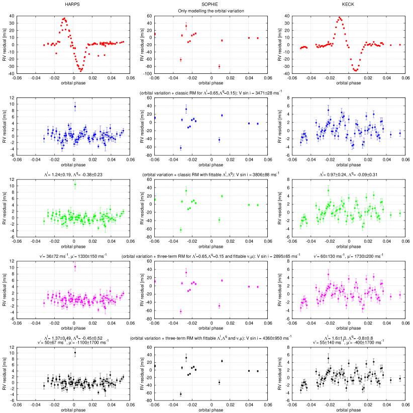
Figure 5: Residuals of the Doppler data for HD 189733, computed in the vicinity of the transit epoch, corresponding to zero abscissa. Each raw of plots corresponds to a best fitting model labelled above the raw, together with the main best fitting parameters. See text for a detailed discussion.

In Fig. 5 we show RV residuals corresponding to different models, in the vicinity of the transit, and separately for the HARPS, SOPHIE, and Keck datasets. We can see that the RM effect is obvious, its curve is well sampled and measured with high accuracy both by HARPS and Keck, whereas SOPHIE has only sporadic data in this phase range (top raw of plots).

In the second raw we plot RV residuals of the classic RM model with the limb-darkening coefficients fixed at $\Lambda^{\mathrm{l}}=0.65$ and $\Lambda^{\mathrm{q}}=0.15$. These values are close to those adopted by Triaud et al. (2009). And confirming (Triaud et al., 2009), the classic model of the RM effect leaves certain systematic wave-like variation in the residuals, which is clear in HARPS and less clear but noticeable in Keck data. Note that all $4$ HARPS transit runs are plotted over each other in a single graph. Their systematic variation cannot be due to the effects like asteroseismologic oscillations, which would change the shape from one transit to another. This variation definitely reflects an inaccuracy of the classic RM model.

Formally, this variation can be equally fitted by either (i) adjusting the limb-darkening coefficients or by (ii) using the correction terms of (3.4). These ways offer practically equivalent models. The residuals look almost identical for these fits, and in the both cases they leave no significant hints of any other systematic variation (third and fourth raws in Fig. 5). However, in the case (i), their estimations of the limb darkening coefficients appear too different from the theoretically predicted values, and actually do not look physically reasonable. This indicates that the case (ii) is more realistic. In this case we obtain a well-constrained estimations of the coefficients $\nu^{\prime}$ and $\mu^{\prime}$. The value of $\nu^{\prime}$ is close to zero, while $\mu^{\prime}$ appears comparable to $V\sin i$ (see labels in Fig. 5). From (3.11), this value of $\mu^{\prime}$ corresponds to the average width of the spectral lines of $\sim 2/3$ of $V\sin i$, or $\sim 1800$ m/s (before the rotational broadening).

The estimation of $V\sin i$ in the case (ii) is reduced by $\sim 25$ per cent in comparison with the case (i). This reduced value of $\sim 2900$ m/s is significantly smaller than the one obtained by Triaud et al. (2009) with the classic RM model ($\sim 3300$ m/s) and even smaller than the value of $\sim 3100$ m/s, obtained by Cameron et al. (2010) based on the line-profile tomography. We need to emphasize that our model is sensitive to the adopted values of the limb-darkening coefficients, and by increasing of $\Lambda^{\mathrm{l}}$ we would obtain an estimate of $V\sin i$ closer to Cameron et al. (2010). From the other side, Cameron et al. (2010) use only a linear term in their limb-darkening model, so at the current stage it is still unclear, which of the two latter estimates is closer to the truth. It is however definite that all values of $V\sin i$ that rely on the classic RM model are overestimated.

We also tried to fit simultaneously the RM correction and the limb-darkening coefficients (fifth raw in Fig. 5). In this case we obtained an ill-conditioned fit with large uncertainties, and the residuals did not change. However we point out that the coefficient $\nu$ is always determined robustly and with a good accuracy, so it does not seem that there is large correlation between $\nu$ and $\mu$ or between $\nu$ and the limb-darkening coefficients. Also $\nu$ is always consistent with zero within narrow limits. This is exactly what theory predicts, because all Doppler data that we used here are obtained by means of the spectrum modelling rather than by correlating with a template. In fact, a zero value of $\nu$ indicates that these spectral models are of a perfect quality.

7 Conclusions and discussion

This paper represents an attempt to construct more general but still analytic models of the RM effect with a particular focus to an improved practical usability, especially by a third-party analysis work. Although our primary new model (3.4) does not depend on several important restrictions, like the single-line spectrum, or specific line profiles, or small planet, there is still much to be done in this topic. The main vulnerability of this model is that it relies on decompositions in $V\sin i$, requiring it to be small. In fact, we considered both modelling approaches: employ power-series decompositions in $V\sin i$, as in (Hirano et al., 2010), or avoid such decompositions by assuming a simple Gaussian line profile, as in (Boué et al., 2013). However, our most useful results correspond to only the first case. In the second case we did not succeed very much, just showing that the actuality is significantly more complicated than explicated e.g. by Boué et al. (2013). Nevertheless, we believe that our primary model can prove a quick and practical workhorse, because most stars that are involved in planet search programmes are rather quiet, implying that their rotation should be relatively slow.

Also, we do not consider the effect of macro-turbulence, which was considered e.g. by Hirano et al. (2011); Boué et al. (2013), and do not take into account differential rotation of the star. These and more subtle effects are left for future work.

Regardless of all the remaining limitations, we believe that our model can be useful in practice, as it is fully analytic, requires nothing but the Doppler data, and can be applied without detailed knowledge of the spectrum reduction pipelines that depend on a particular practical case. This paper gives a comprehensive set of all necessary formula, and we are going to release their implementation with the next version 3.0 of the PlanetPack package (Baluev, 2013a).

Appendix A Rossiter-McLaughlin anomaly for a small planet, arbitrary rotation velocity, and multi-Gaussian spectra

See Sect. 3 for the details of the approximation method.

A.1 Cross-correlation with a predefined template

Let us assume Gaussian approximation for all our spectra:

$$\mathcal{F}_{\star}(s)=\mathcal{G}_{\bm{\beta}_{\star}}(s,\textbf{{u}},\textbf{{c}}_{\star}),\qquad\mathcal{F}_{\mathrm{p}}(s)=\mathcal{G}_{\bm{\beta}_{\mathrm{p}}(s)}(s-s_{\mathrm{p}}(s),\textbf{{u}},\textbf{{c}}),\qquad\mathcal{F}_{\mathrm{T}}(s)=\mathcal{G}_{\bm{\beta}_{\mathrm{T}}}(s,\textbf{{u}}_{\mathrm{T}},\textbf{{c}}_{\mathrm{T}}).$$ (A.1)

Here the spectral lines positions u are the same for $\mathcal{F}_{\star}$ and $\mathcal{F}_{\mathrm{p}}$, but we admit that they may be slightly different from those used in the template, $\textbf{{u}}_{\mathrm{T}}=\textbf{{u}}+\Delta\textbf{{u}}$. In this manner we model possible template imperfections.

Using the expression (2.26) and (2.22), and approximating all slowly varying functions like $M_{0}^{\star}(s)$, and $\sigma_{\star}(s)$ in the vicinity of each line by a constant, we can transform equation (2.6) to the following:

$$0=\left\langle\mathcal{F}_{\star}\mathcal{F}_{\mathrm{T}}^{\prime}\right\rangle\simeq\sum_{i=1}^{N}M_{0}^{\star}(u_{i})c_{\star,i}c_{\mathrm{T},i}\mathcal{G}_{\sqrt{\beta_{i}^{2}+\sigma_{\star}^{2}+\beta_{\mathrm{T},i}^{2}}}^{\prime}(-\Delta u_{i})=\frac{1}{\sqrt{2\pi}}\sum_{i=1}^{N}\frac{M_{0}^{\star}(u_{i})c_{\star,i}c_{\mathrm{T},i}\Delta u_{i}}{(\beta_{i}^{2}+\sigma_{\star}^{2}+\beta_{\mathrm{T},i}^{2})^{3/2}}+\mathcal{O}(\Delta\textbf{{u}}^{3}).$$ (A.2)

If $\Delta u_{i}=0$ than this equality is satisfied automatically, and otherwise it sets a balancing requirement for $\Delta u_{i}$. For example, it is illegal if all $\Delta u_{i}$ only introduce a common systematic shift, because this would just result in a biasing effect on the RV absolute zero point, which does not affect relative RV measurements that we consider here.

Various quantities appearing in (2.12) can be expressed analogously. Dropping the terms having relative magnitude $\mathcal{O}(\Delta\textbf{{u}}^{2})$ and smaller, we obtain:

$$\left\langle\mathcal{F}_{\mathrm{p}}\mathcal{F}_{\mathrm{T}}^{\prime}\right\rangle \simeq \sum_{i=1}^{N}M_{0}(u_{i})c_{i}c_{\mathrm{T},i}\mathcal{G}_{\sqrt{\beta_{i}^{2}+\sigma_{\mathrm{p}}^{2}(u_{i})+\beta_{\mathrm{T},i}^{2}}}^{\prime}(s_{\mathrm{p}}(u_{i}))-\sum_{i=1}^{N}M_{0}(u_{i})c_{i}c_{\mathrm{T},i}\Delta u_{i}\mathcal{G}_{\sqrt{\beta_{i}^{2}+\sigma_{\mathrm{p}}^{2}(u_{i})+\beta_{\mathrm{T},i}^{2}}}^{\prime\prime}(s_{\mathrm{p}}(u_{i})),$$

$$\left\langle\mathcal{F}_{\star}\mathcal{F}_{\mathrm{T}}^{\prime\prime}\right\rangle \simeq -\frac{1}{\sqrt{2\pi}}\sum_{i=1}^{N}\frac{M_{0}^{\star}(u_{i})c_{\star,i}c_{\mathrm{T},i}}{(\beta_{i}^{2}+\sigma_{\star}^{2}(u_{i})+\beta_{\mathrm{T},i}^{2})^{3/2}},\qquad\hat{s}\simeq-\frac{\left\langle\mathcal{F}_{\mathrm{p}}\mathcal{F}_{\mathrm{T}}^{\prime}\right\rangle}{\left\langle\mathcal{F}_{\star}\mathcal{F}_{\mathrm{T}}^{\prime\prime}\right\rangle}.$$ (A.3)

As we can see, the formulae for multiline spectra are significantly more complicated than for the single-line case considered in previous works. But before discussing them, let us consider the case of a single line. For $N=1$ the formulae (A.3) reduce to

$$\hat{s}\simeq-fs_{\mathrm{p}}\frac{c}{c_{\star}}\left(\frac{\beta_{\star}^{2}+\beta_{\mathrm{T}}^{2}}{\beta_{\mathrm{p}}^{2}+\beta_{\mathrm{T}}^{2}}\right)^{\frac{3}{2}}\exp\left(-\frac{s_{\mathrm{p}}^{2}}{2(\beta_{\mathrm{p}}^{2}+\beta_{\mathrm{T}}^{2})}\right),\qquad f=\frac{M_{0}}{M_{0}^{\star}}.$$ (A.4)

This appears almost equivalent to the formula (15) by (Boué et al., 2013). As they also fit the template via $\beta_{\mathrm{T}}$, it becomes equal to $\beta_{\star}$ in their work. We obtain an additional factor of $c/c_{\star}$, the ratio of line intensities in the spectra of rotating star and stellar surface at rest. This ratio does not appear in Boué et al. (2013). We believe this factor might be “lost” because they put an additional condition that $\mathcal{F}_{\star}$ and $\mathcal{F}_{\mathrm{p}}$ both should be pre-normalized, and consider them containing just a single line without even a continuum. This looks illegal, because the spectrum normalization mainly depends on its continuum, and not on the lines. Because line intensity $a_{\star}$ may be different from $a$, the normalizations of $\mathcal{F}_{\star}$ and $\mathcal{F}_{\mathrm{p}}$ become different and cannot not be directly combined in $\mathcal{F}_{\mathrm{t}}$. Instead, it is better to consider unnormalized spectra treated as energy distributions, as we do in the present work. In this case we still do not need to take care of the continuum, but spectra normalizations become mutually consistent.

The multiline approximation (A.3) appears even more complicated. First, the summation over the lines in (A.3) should likely introduce additional broadening effect in comparison with the single-line formula (A.4). Second, the multiline expression (A.3) contains terms depending on $\Delta u_{i}$. This should introduce additional effect that depends on the quality of the template. This effect was not characterized previously, because it can be only revealed when working with the multiline model. Note that the functional shape of this template imperfection effect should be significantly different from the single-line formula (A.4). Instead of the dependence on $s_{\mathrm{p}}$ like $G^{\prime}(s_{\mathrm{p}})\sim s_{\mathrm{p}}\exp(-s_{\mathrm{p}}^{2})$ (qualitatively), we should now deal with something like $G^{\prime\prime}(s_{\mathrm{p}})\sim(s_{\mathrm{p}}^{2}-1)\exp(-s_{\mathrm{p}}^{2})$. In fact, we cannot even guarantee that $\hat{s}=0$ for $s_{\mathrm{p}}=0$ in this case: template imperfections introduce a bias.

Unfortunately, this type of models is very difficult for practical use. It requires a comprehencive knowledge of deep internals of the spectra processing technique applied in the particular case. This is not available for authors who want to e.g. reanalyse some public Doppler data. Moreover, even when such a knowledge is available, the multiline model becomes mathematically complicated. Therefore, in this work we do not consider this type of approximations in more details.

We do not give detailed expressions for the case in which the CCF is fitted by a Gaussian, described by the formula (2.15). Clearly, the final formulae for this case should be much more complicated than (A.3). Note that due to the template imperfections, $\Delta\textbf{{u}}$, appearing for multiline spectra, the term $\langle\mathcal{F}_{\star}\mathcal{F}_{\mathrm{T}}^{\prime\prime\prime}\rangle$ in (2.15) is non-zero even for symmetric lines and thus cannot be neglected.

A.2 Cross-correlation with an out-of-transit stellar spectrum or parametric modelling of the stellar spectrum (iodine cell technique)

Now we should just substitute $\mathcal{F}_{\star}$ in place of $\mathcal{F}_{\mathrm{T}}$ in the formulae presented above. Formulae (A.3) turn into

$$\left\langle\mathcal{F}_{\mathrm{p}}\mathcal{F}_{\star}^{\prime}\right\rangle\simeq\sum_{i=1}^{N}M_{0}(u_{i})M_{0}^{\star}(u_{i})c_{i}c_{\star,i}\mathcal{G}_{\sqrt{2\beta_{i}^{2}+\sigma_{\mathrm{p}}^{2}(u_{i})+\sigma_{\star}^{2}(u_{i})}}^{\prime}(s_{\mathrm{p}}(u_{i})),\quad\left\langle\mathcal{F}_{\star}\mathcal{F}_{\star}^{\prime\prime}\right\rangle\simeq-\frac{1}{4\sqrt{\pi}}\sum_{i=1}^{N}\frac{M_{0}^{\star}(u_{i})^{2}c_{\star,i}^{2}}{(\beta_{i}^{2}+\sigma_{\star}^{2}(u_{i}))^{3/2}},\quad\hat{s}\simeq-\frac{\left\langle\mathcal{F}_{\mathrm{p}}\mathcal{F}_{\star}^{\prime}\right\rangle}{\left\langle\mathcal{F}_{\star}\mathcal{F}_{\star}^{\prime\prime}\right\rangle}.$$ (A.5)

Here the template lines misplacements $\Delta u_{i}$ all vanish, because the new template coincides with $\mathcal{F}_{\star}$. Doppler anomaly can be expressed as follows:

$$\hat{s}\simeq-\left[\sum_{i=1}^{N}\frac{M_{0}(u_{i})M_{0}^{\star}(u_{i})c_{i}c_{\star,i}}{(\beta_{\mathrm{p}}^{2}(u_{i})+\beta_{\star}^{2}(u_{i}))^{3/2}}s_{\mathrm{p}}(u_{i})\exp\left(-\frac{s_{\mathrm{p}}^{2}(u_{i})}{2(\beta_{\mathrm{p}}^{2}(u_{i})+\beta_{\star}^{2}(u_{i}))}\right)\right]\left/\left(\sum_{i=1}^{N}\frac{M_{0}^{\star}(u_{i})^{2}c_{\star,i}^{2}}{(2\beta_{\star}^{2}(u_{i}))^{3/2}}\right)\right..$$ (A.6)

Now the formula is more simple than (A.3): the template imperfections are irrelevant, and the RM effect is not biased: $s_{\mathrm{p}}=0$ implies $\hat{s}=0$. However, it still requires a very detailed knowledge of the stellar spectrum.

For a single line, we obtain

$$\hat{s}\simeq-fs_{\mathrm{p}}\frac{c}{c_{\star}}\left(\frac{2\beta_{\star}^{2}}{\beta_{\mathrm{p}}^{2}+\beta_{\star}^{2}}\right)^{\frac{3}{2}}\exp\left(-\frac{s_{\mathrm{p}}^{2}}{2(\beta_{\mathrm{p}}^{2}+\beta_{\star}^{2})}\right),\qquad f=\frac{M_{0}}{M_{0}^{\star}}.$$ (A.7)

This basically agrees with Boué et al. (2013) and Hirano et al. (2010). But again, the summations in (A.6) should introduce an additional broadening effect in comparison with (A.7).