Thermal and electrical properties of a solid through Fibonacci oscillators

Abstract

We investigate the thermodynamics of a crystalline solid applying $q$-deformed algebra of Fibonacci oscillators through the generalized Fibonacci sequence of two real and independent deformation parameters $q_{1}$ and $q_{2}$. We based part of our study on both Einstein and Debye models, exploring primarily $(q_{1},q_{2})$-deformed thermal and electric conductivities as a function of Debye specific heat. The results revealed that $q$-deformation acts as a factor of disorder or impurity, modifying the characteristics of a crystalline structure. Specially, one may find the possibility of adjusting the Fibonacci oscillators to describe the change of thermal and electrical conductivities of a given element as one inserts impurities. Each parameter can be associated to different types of deformations such as disorders and impurities.

I Introduction

The interaction between atoms allows propagation of elastic waves in the solid medium which can be both transverse and longitudinal. If the oscillations of the atoms around the equilibrium positions are small, which should occur at lower temperatures, the potential energy of interaction can be approximated by a quadratic form of the displacements of atoms from their equilibrium positions. A crystalline solid, whose atoms interact according to this potential, is called a harmonic solid. In harmonic solids, elastic waves are harmonics and the normal modes of vibration in crystalline solids kit2 . A large number of phenomena involve quantum mechanical motion, in particular thermally-activated particles, obeying the $T^{3}$ law. Thermal excitations in the system are responsible for phonon excitation patt ; hua .

The study conducted by Anderson, Lee and Elliot ande ; lee ; ell shows that the presence of defects or impurities in a crystal modifies the electrostatic potential in their neighborhood, breaking the translational symmetry of the periodic potential. This perturbation can produce electronic wave functions located near the impurity, ceasing to be propagated throughout the crystal.

A possible way to generate a deformed version of the classical statistical mechanics consists in replacing the Gibbs-Boltzmann distribution by a deformed version. In this respect it is postulated a form of deformed entropy tsalis which implies a generalized theory of thermodynamics.

We apply the $q$-deformation in the models of Einstein and Debye bri2 ; bri3 ; bri6 , and our results show that the factor $q$ acts as an impurity, modifying the thermodynamic quantities such as entropy, specific heat, thermal conductivity, etc.

In this work we insert the given parameters of deformation $q_{1}$ and $q_{2}$, called Fibonacci oscillators arik2 , which is a formalism recently proposed in the $q$-calculation that has been investigated in aba ; amg1 ; bri4 . They provide a unification of quantum oscillators with quantum groups, keeping the degeneration property of the spectrum invariant under the symmetries of the quantum group bie1 ; mac ; fuc ; erz ; anat . The quantum algebra with two deformation parameters may have a greater flexibility when it comes to applications in realistic phenomenological physical models dao ; gong and may increase interest in physical applications.

The paper is organized as follows. In Sec. II we present the deformed algebra. In Sec. III we apply the Fibonacci oscillators, in the Einstein III.1 and Debye III.2 models, and finally, in Sec. (IV) we make our final comments.

II Algebra of the Fibonacci oscillators

It is well-known that the generalization of integers in general is given by a sequence. A basic procedure in $q$-algebra jac1 is a generalization of integers. Two well-known ways to describe a sequence are the arithmetic and geometric progressions. A simple generalization that encompasses both of is the Fibonacci sequence, which as we know is a linear combination where the third number is the sum of two predecessors, and so on. Here, the numbers are in that sequence of generalized Fibonacci oscillators, where new parameters $(q_{1},q_{2})$ are introduced. Thus, the generalized spectrum may be given by the whole Fibonacci number.

The algebraic symmetry of the quantum oscillator is defined by the Heisenberg algebra in terms of the annihilation and creation operators $c$, $c^{\dagger}$, respectively, and the number operator $N$ aba ; lav1 via

$$c_{i}c_{i}^{\dagger}-q_{1}^{2}c_{i}^{\dagger}c_{i}=q_{2}^{2n_{i}}\qquad\mbox{and}\qquad c_{i}c_{i}^{\dagger}-q_{2}^{2}c_{i}^{\dagger}c_{i}=q_{1}^{2n_{i}},$$ (1)

$$[N,c^{\dagger}]=c^{\dagger},\qquad\qquad[N,c]=-c.$$ (2)

In addition, the operators obey the relations

$$c^{\dagger}c=[N],\;\;\qquad cc^{\dagger}=[1+N],$$ (3)

$$[1+n_{i,q_{1},q_{2}}]=q_{1}^{2}[n_{i,q_{1},q_{2}}]+q_{2}^{2n_{i}},\;\quad\mbox{or}\quad\;[1+n_{i,q_{1},q_{2}}]=q_{2}^{2}[n_{i,q_{1},q_{2}}]+q_{1}^{2n_{i}}.$$ (4)

The oscillator bie1 ; mac allows us to write the $(q_{1},q_{2})$-deformed Hamiltonian anat as follows

$${\cal H}=\frac{1}{2}\Big{\{c,c^{\dagger}\Big{\}}}.$$ (5)

The Fibonacci basic number is defined by arik

$$[n_{i,q_{1},q_{2}}]=c_{i}^{\dagger}c_{i}=\frac{q_{2}^{2n_{i}}-q_{1}^{2n_{i}}}{q_{2}^{2}-q_{1}^{2}},$$ (6)

where $q_{1}$ and $q_{2}$ are real positive and independent parameters of deformation.

III Application of Fibonacci Oscillators

III.1 ($q_{1},q_{2}$)-deformed Einstein solid

We consider the solid in contact with a thermal reservoir at temperature $T$, where we have $n_{j}$ labeling the $j$-th oscillator Given a microscopic state $\{n_{j}\}=\{n_{1},n_{2},\ldots,n_{N}\}$, the energy of this state can be written as,

$$E\{n_{j}\}=\displaystyle\sum_{j=1}^{\infty}\left(n_{j}+\frac{1}{2}\right)\hbar\omega_{E},$$ (7)

where $\omega_{E}$ is the Einstein frequency characteristic. We can obtain $(q_{1},q_{2})$-deformed energies from the definition of the Hamiltonian (5), and the definitions provided earlier,

$$E_{n_{i,q_{1},q_{2}}}=\frac{\hbar\omega_{E}}{2}\Big{(}[n_{i,q_{1},q_{2}}]+[n_{i,q_{1},q_{2}}+1]\Big{)}=\frac{\hbar\omega_{E}}{2}+\frac{\hbar\omega_{E}\left(2\ln(q_{2})-2\ln(q_{1})\right)n}{q_{2}^{2}-q_{1}^{2}},$$ (8)

and when $q_{1}=q_{2}=1$, we recover the usual spectrum

$$E_{n}=\frac{\hbar\omega_{E}}{2}\left(2n+1\right).$$ (9)

With the result of the Eq.(8), we can rewrite the partition function in the form,

$$\Xi_{(q_{1},q_{2})}=\Bigg{\{}\displaystyle\sum_{n=0}^{\infty}\exp\left[-\beta E_{n_{i,q_{1},q_{2}}}\right]\Bigg{\}}^{N}=\Xi_{(1,q_{1},q_{2})}^{N},$$ (10)

where

$$\Xi_{(1,q_{1},q_{2})}=\frac{q_{1}^{2\alpha}}{\exp\left(\frac{\alpha(q_{1}^{2}-q_{2}^{2})}{2}\right)(q_{1}^{2\alpha}-q_{2}^{2\alpha})}.$$ (11)

We define a $(q_{1},q_{2})$-deformed Einstein function $E(\alpha)_{q_{1},q_{2}}$,

$$E(\alpha)_{q_{1},q_{2}}=\left(\frac{2\alpha q_{1}q_{2}[\ln(q_{1})-\ln(q_{2})]}{(q_{1}^{2\alpha}-q_{2}^{2\alpha})}\right)^{2},\qquad\mbox{where}\qquad\alpha=\left(\frac{\Theta_{E}}{T(q_{1}^{2}-q_{2}^{2})}\right).$$ (12)

As one knows $\Theta_{E}$ is the Einstein temperature, defined by

$$\Theta_{E}=\left(\frac{\hbar\omega_{E}}{\kappa_{B}}\right),$$ (13)

and $\kappa_{B}$ is the Boltzmann constant. When $q_{1}=q_{2}\to 1$, we have the undeformed function

$$E(\alpha^{*})=\frac{\exp(\alpha^{*})\alpha^{2*}}{(\exp{\alpha^{*}}-1)^{2}},\qquad\;\mbox{where}\qquad\alpha^{*}=\frac{\Theta_{E}}{T}.$$ (14)

We can determine ($q_{1},q_{2}$)-deformed the Helmholtz free energy per oscillator and entropy, respectively

$$f_{q_{1},q_{2}}=-\frac{1}{\beta}\;\displaystyle\lim_{N\to\infty}\frac{1}{N}\ln\Xi_{(q_{1},q_{2})}=-\kappa_{B}T\ln\left[\frac{q_{1}^{2\alpha}}{\exp\left(\frac{\alpha(q_{1}^{2}-q_{2}^{2})}{2}\right)(q_{1}^{2\alpha}-q_{2}^{2\alpha})}\right].$$ (15)

$$S_{q_{1},q_{2}} = -\frac{\partial f_{q_{1},q_{2}}}{\partial T}=\kappa_{B}\Biggl{\{}\ln\Bigg{[}\frac{q_{1}^{2\alpha}}{\exp\Big{(}\frac{\alpha(q_{1}^{2}-q_{2}^{2})}{2}\Big{)}(q_{1}^{2\alpha}-q_{2}^{2\alpha})}\Bigg{]}+$$ (16)

$$+ \Bigg{[}\frac{2\alpha q_{2}^{2\alpha}(\ln(q_{1})-\ln(q_{2}))}{(q_{1}^{2\alpha}-q_{2}^{2\alpha})}+\frac{\alpha(q_{1}^{2}-q_{2}^{2})}{2}\Bigg{]}\Biggl{\}}.$$

In Fig. (1) is shown the behavior of the entropy as a function of temperature variation. We observe that all the curves have the same behavior at low temperature. However, as the temperature increases the role of the $q$-deformation becomes much more evident. For instance, note that $q_{2}$ tends do decrease the entropy more than $q_{1}$. As we anticipated, these parameters can play different roles. While one can affect disorders the other may control impurities.

Now we determine ($q_{1},q_{2}$)-deformed specific heat, and we can do it by inserting the Einstein function $E(\alpha)_{q_{1},q_{2}}$, defined by Eq.(12), into equation below

$$c_{V_{q_{1},q_{2}}}(T)=T\left(\frac{\partial S_{q_{1},q_{2}}}{\partial T}\right)=\kappa_{B}\,\left(\frac{2\alpha q_{1}q_{2}[\ln(q_{1})-\ln(q_{2})]}{(q_{1}^{2\alpha}-q_{2}^{2\alpha})}\right)^{2}.$$ (17)

$$c_{V_{q_{1},q_{2}}}(T)=3\kappa_{B}E(\alpha)_{q_{1},q_{2}}.$$ (18)

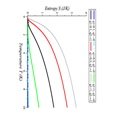
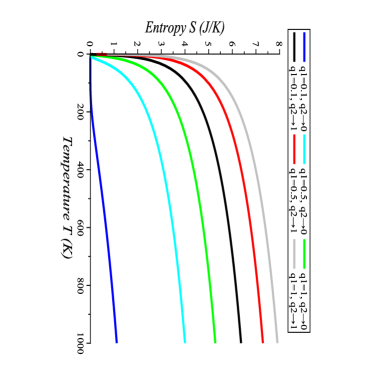
Figure 1: ${q_{1},q_{2}}$-deformed entropy $S_{q_{1},q_{2}}$ vs temperature T in the following intervals: (T=$0,\cdots,10K$) (left) and (T=$0,\cdots,1000K$) (right)

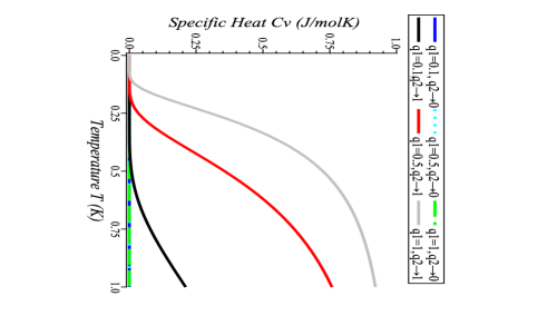
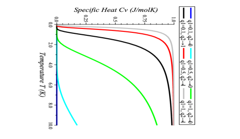
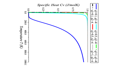
Figure 2: ${q_{1},q_{2}}$-deformed specific heat $c_{V_{q_{1},q_{2}}}$ vs temperature T in the following intervals: (T=$0,\cdots,1K$) (left), (T=$0,\cdots,10K$) (center) and (T=$0,\cdots,1000K$) (right).

The complete behavior is depicted in Fig. (2). One should note that when $T\gg\Theta_{E}$, and thus the ratio $\alpha=\frac{\Theta_{E}}{T}\ll 1$, and $\Theta_{E}$ around $100K$ for common crystals, one recovers the classical result $c_{V_{q_{1},q_{2}}}\to 3\kappa_{B}$, known as the Dulong-Petit law. However, for sufficiently low temperatures, where $T\ll\Theta_{E}$ and therefore $\alpha\gg 1$, specific heat decreases exponentially with temperature patt , as

$$c_{V}\rightarrow\kappa_{B}\left(\frac{\theta_{E}}{T}\right)^{2}\exp\left(-\frac{\theta_{E}}{T}\right).$$ (19)

In general, the invariance of specific heat at high temperatures and its decrease at low temperatures show that the Einstein model is in agreement with experimental results. However, at sufficiently low temperatures, specific heat does not experimentally follow the exponential function given in Eq.(19). As for the $(q_{1},q_{2})$-deformed case we see a significant change in the curves at intermediate temperatures.

III.2 ($q_{1},q_{2}$)-deformed Debye solid

Corrections of Einstein model are given by the Debye model, allowing us to integrate from a continuous spectrum of frequencies up to the Debye frequency $\omega_{D}$, giving the total number of normal modes of vibration patt ; hua ; kit2

$$\int_{0}^{\omega_{D}}g(\omega)d\omega=3N,$$ (20)

where $g(\omega)d\omega$ denotes the number of normal modes of vibration whose frequency is in the range $(\omega,\omega+d\omega)$. The function $g(\omega)$, can be given in terms of the Rayleigh expression as follows

$$8\pi\left(\frac{1}{\lambda}\right)^{2}d\left(\frac{1}{\lambda}\right)=\frac{\omega^{2}d\omega}{\pi^{2}c^{3}},$$ (21)

where $c$ is the speed of light and $\lambda$ wavelength. The expected energy value of the Planck oscillator with frequency $\omega_{s}$ is

$$\langle E_{s}\rangle=\frac{\hbar\omega_{s}}{\exp\left(\frac{\hbar\omega_{s}}{\kappa_{B}T}\right)-1}.$$ (22)

Using Eqs.(21) and (22), we obtain the energy density associated with the frequency range $(\omega,\omega+d\omega)$,

$$u(\omega)d\omega=\frac{\hbar}{\pi^{2}c^{3}}\frac{\omega^{3}d\omega}{\exp\left(\frac{\hbar\omega}{\kappa_{B}T}\right)-1}.$$ (23)

To obtain the number of photons between $\omega$ and $\omega+d\omega$, one makes use of the volume of the region on the phase space patt , which results in

$$g(\omega)d\omega\approx\frac{2V}{h^{3}}\left[4\pi\left(\frac{\hbar\omega}{c}\right)^{2}\left(\frac{\hbar d\omega}{c}\right)\right]=\frac{V\omega^{2}d\omega}{\pi^{2}c^{3}}.$$ (24)

Thus, replacing Eq.(24) into Eq.(21), we can write the specific heat for any temperature. We now apply ($q_{1},q_{2}$)-deformation in the same way as in Eq.(18),

$$c_{V_{q_{1},q_{2}}}(T)=3\kappa_{B}D(\alpha_{0_{q_{1},q_{2}}}),$$ (25)

where $D(\alpha_{0_{q_{1},q_{2}}})$ is the ($q_{1},q_{2}$)-deformed Debye function, defined by

$$D(\alpha_{0_{q_{1},q_{2}}})=\frac{3}{(\alpha_{0_{q_{1},q_{2}}})^{3}}\int_{0}^{\alpha_{0_{q_{1},q_{2}}}}\frac{\alpha^{4}\exp{(\alpha)}}{[\exp(\alpha)-1]^{2}}d\alpha,\qquad\;{\alpha_{0_{q_{1},q_{2}}}}=\frac{\hbar\omega_{D_{q_{1},q_{2}}}}{\kappa_{B}T}=\frac{\theta_{D_{q_{1},q_{2}}}}{T},$$ (26)

$$\omega_{D_{q_{1},q_{2}}}=2\omega_{D}\left(\frac{\ln(q_{2})-\ln(q_{1})}{q_{2}^{2}-q_{1}^{2}}\right),$$ (27)

where $\omega_{D_{q_{1},q_{2}}}$ and $\theta_{D_{q_{1},q_{2}}}$, are the $(q_{1},q_{2})$-deformed Debye frequency and temperature, respectively, and $\omega_{D}$ is the Debye frequency characteristic. Integrating Eq.(26) by parts one finds

$$D(\alpha_{0_{q_{1},q_{2}}})=-\frac{3{\alpha_{0_{q_{1},q_{2}}}}}{\exp({\alpha_{0_{q_{1},q_{2}}}})-1}+\frac{12}{\alpha_{0_{q_{1},q_{2}}}^{3}}\int_{0}^{\alpha_{0_{q_{1},q_{2}}}}{\frac{\alpha^{3}d\alpha}{\exp(\alpha)-1}},$$ (28)

which can be integrated out to give the full expression

$$D(\alpha_{0_{q_{1},q_{2}}}) = -\frac{3{\alpha_{0_{q_{1},q_{2}}}}}{\exp({\alpha_{0_{q_{1},q_{2}}}})-1}+\frac{12}{\alpha_{0_{q_{1},q_{2}}}^{3}}\Bigg{\{}-\frac{\pi^{4}}{15}-\frac{\alpha_{0_{q_{1},q_{2}}}^{4}}{4}+\alpha_{0_{q_{1},q_{2}}}^{3}\ln[1-\exp(\alpha_{0_{q_{1},q_{2}}})]$$ (29)

$$+ 3\alpha_{0_{q_{1},q_{2}}}^{2}{\rm Li}_{2}[\exp(\alpha_{0_{q_{1},q_{2}}})]-6\alpha_{0_{q_{1},q_{2}}}{\rm Li}_{3}[\exp(\alpha_{0_{q_{1},q_{2}}})]+6{\rm Li}_{4}[\exp(\alpha_{0_{q_{1},q_{2}}})]\Bigg{\}},$$

where

$${\rm Li}_{n}(z)=\displaystyle\sum_{k=0}^{\infty}{\frac{z^{n}}{k^{n}}},$$ (30)

is the polylogarithm function. For $T\gg\theta_{D_{q}}$, $\alpha_{0{(q_{1},q_{2})}}\ll 1$, then the function $D(\alpha_{0})_{q}$ can be expressed in a power series in $\alpha_{0_{q}}$

$$D(\alpha_{0})_{q}=1-\frac{\alpha_{0_{q}}^{2}}{20}+\cdots$$ (31)

so that for

$$T\to\infty\;,\qquad c_{V{q}}\to 3\kappa_{B}.$$ (32)

On the other hand, for $T\ll\theta_{D_{q}}$, $\alpha_{0_{q}}\gg 1$, then we can write function $D(\alpha_{0})_{q}$ as

$$\frac{12}{\alpha_{0_{q}}^{3}}\displaystyle\int_{0}^{\infty}{\frac{\alpha^{3}d\alpha}{\exp(\alpha)-1}+O[\exp(-\alpha_{0_{q}})]},$$ (33)

$$\approx\frac{4\pi^{4}}{5\alpha_{0_{q}}^{3}}=\frac{4\pi^{4}}{5}\left(\frac{T}{\theta_{D_{q}}}\right)^{3}.$$ (34)

Thus, as in the usual Debye solid, the low-temperature specific heat in a q-deformed Debye solid is proportional to $T^{3}$, due to phonon excitation, a fact that is in agreement with experiments. Thus, let us express the ($q_{1},q_{2}$)-deformed specific heat for low temperatures as follows:

$$c_{V_{q_{1},q_{2}}}=\frac{12\pi^{4}\kappa_{B}}{5}\left(\frac{T}{\theta_{D_{q_{1},q_{2}}}}\right)^{3}=1944\left(\frac{T}{\theta_{D_{q_{1},q_{2}}}}\right)^{3}\frac{J}{molK}.$$ (35)

For the ($q_{1},q_{2}$)-deformed case one can observe the changes that occur with Debye temperature, specific heat, thermal and electrical conductivies. By using the relationship established for thermal conductivity $(\kappa)$ — see zim , we obtain

$$\kappa=\frac{1}{3}C_{V}vl,$$ (36)

where $v$ is the average velocity of the particle, $C_{V}$ is the molar heat capacity and $l$ is the space between particles. We can deduce a relationship between the thermal and electrical $(\sigma)$ conductivities through the elimination of $l$ (as $\sigma=\frac{ne^{2}l}{mv}$, where $m$ is the electron mass, $n$ is the number of electrons per volume unit and $e$ is the electron charge), such that

$$\frac{\kappa}{\sigma}=\frac{1}{3}\frac{C_{V}mv^{2}}{ne^{2}}.$$ (37)

In a classical gas the average energy of a particle is $\frac{1}{2}mv^{2}=\frac{3}{2}\kappa_{B}T$, whereas the heat capacity is $\frac{3}{2}n\kappa_{B}$, so that

$$\frac{\kappa}{\sigma}=\frac{3}{2}\left(\frac{\kappa_{B}}{e}\right)^{2}T.$$ (38)

The ratio $\frac{\kappa}{\sigma T}$ is called the Lorenz number and should be a constant, independent of the temperature and the scattering mechanism. This is the famous Wiedemann-Franz law, which is often well satisfied experimentally, and the Lorenz number correctly given zim . By using the $(q_{1},q_{2})$-deformed relations presented above, we start from Eqs.(36) and (38) to determine the important relations for $(q_{1},q_{2})$-deformed thermal and electrical conductivities

$$\kappa_{q_{1},q_{2}}=\frac{\kappa c_{V_{q_{1},q_{2}}}}{c_{V}}\qquad\qquad\mbox{and}\qquad\qquad\sigma_{q_{1},q_{2}}=\frac{\kappa_{{q_{1},q_{2}}}\sigma}{\kappa}.$$ (39)

Recall that to compute these deformed quantities in terms of the specific heat $c_{V_{q_{1},q_{2}}}$ we make use of Eq.(29) and its suitable limits. We present in Tab. (1), changes that occur with the Debye temperature, specific heat, thermal conductivity and electrical conductivity, of some chemical elements.

Element	$\theta_{D_{q}}^{(a)}$			$C_{V_{q}}^{(b)}$			$\kappa_{q}^{(c)}$			$\sigma_{q}^{(d)}$
	$q_{2}$=1	$q_{2}$=0.5	$q_{2}$=0.1	$q_{2}$=1	$q_{2}$=0.5	$q_{2}$=0.1	$q_{2}$=1	$q_{2}$=0.5	$q_{2}$=0.1	$q_{2}$=1	$q_{2}$=0.5	$q_{2}$=0.1
Pb	105	194	488	4.53$\times 10^{4}$	7.2$\times 10^{3}$	450	0.35	0.06	0.003	0.48	0.076	0.00477
Bi	119	220	554	3.11$\times 10^{4}$	4.9$\times 10^{3}$	309	0.08	0.013	0.0008	0.09	0.0143	0.00089
Yb	120	222	558	3.04$\times 10^{4}$	4.8$\times 10^{3}$	302	0.35	0.055	0.0035	0.38	0.06	0.0038
Pt	240	444	1116	3.8$\times 10^{3}$	601	38	0.72	0.11	0.007	0.96	0.15	0.01
Pd	274	506	1275	2.55$\times 10^{3}$	404	25	0.72	0.11	0.007	0.95	0.15	0.01
Y	280	518	1302	2.39$\times 10^{3}$	379	24	0.17	0.027	0.002	0.17	0.027	0.002
Zn	327	604	1521	1.5$\times 10^{3}$	238	15	1.16	0.18	0.01	1.69	0.27	0.017
Mn	410	758	1907	762	121	7.6	0.08	0.013	0.0008	0.072	0.011	0.0007
Ti	420	776	1954	708	112	7	0.46	0.073	0.005	0.23	0.04	0.002
Ni	450	832	2093	576	91	5.7	0.91	0.14	0.009	1.43	0.23	0.014
Fe	470	869	2186	506	80	5	0.80	0.13	0.008	1.02	0.016	0.01
Os	500	924	2326	420	66	4.2	0.88	0.14	0.009	1.10	0.17	0.011
Ru	600	1109	2791	243	38	2.4	1.17	0.18	0.01	1.35	0.22	0.013
Cr	630	1165	2931	210	33	2	0.94	0.15	0.009	0.78	0.12	0.0077
Si	645	1192	3000	196	31	1.9	1.48	0.23	0.015	-	-	-
Be	1440	2662	6698	18	2.8	0.17	2.00	0.32	0.02	3.08	0.49	0.03
C	2230	4122	10374	4.7	0.75	0.048	1.29	0.2	0.01	-	-	-

Table 1: Chemical elements and their respective Debye temperatures ^a$(K)$, Specific heat ^b$\left(\frac{J}{molK}\right)$, thermal conductivity ^c$\left(\frac{W}{cm\dot{K}}\right)$, Electrical conductivity ^d$(ohm\cdot cm)^{-1}\times 10^{5}$, for $T=300K$ and the $q$-deformed values for $q_{1}\to 1$ and $q_{2}=0.1$, $q_{2}=0.5$ and $q_{2}=1$. kit2

For illustration purposes, we choose iron (Fe) and chromium (Cr), two materials that can be employed in many areas of interest. In Figs.(3, 4) we present deformed values of $Fe$ ($Fe_{q-def}$) (black) and $Cr$ ($Cr_{q-def}$) (green), for values $q_{1}=1$ and $q_{2}=0.1,\cdots,1$, where for this range we assume the maximum deformation ($q_{1}=1$ and $q_{2}=0.1$) and the pure element (bulk) ($q_{1}=1$ and $q_{2}=1$). The other elements are represented by colors and indicated in the very figure.

On the left side of the Fig.(3), we can observe that before reaching their limits, black and green curves can assume the values of Debye temperatures ($\theta_{D}$) of other elements. The $Fe_{q-def}$ e.g., equates to: beryllium (Be) when $q_{2}\approx 0.23$, chromium (bulk) (Cr) $q_{2}\approx 0.75$ and osmium (Os) $q_{2}\approx 0.94$. On the right, we have the behavior of the curves obtained for the specific heat $c_{V}$. We note that the behavior is quite different from the previous curves $\theta_{D}$, i.e., the curves start at lower values (maximum deformation) until they reach their pure values. Having $Fe_{q-def}$ as an example again, it is possible to see, as it reaches the value of specific heat capacity of all the elements, including $Cr$ (bulk) when $q_{2}\approx 0.74$.

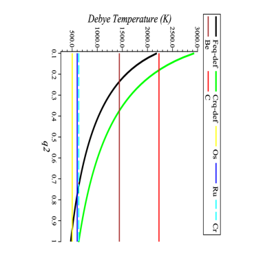
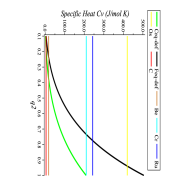
Figure 3: Debye Temperature $\theta_{D}$ depending on the variation $q_{2}=0.1,\cdots,1$ and $q_{1}=1$, (left). Specific Heat $c_{V}$ depending on the variation $q_{2}=0.1,\cdots,1$ and $q_{1}=1$, (right)

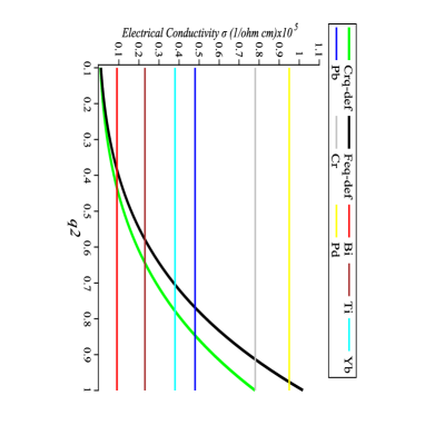
Figure 4: Thermal Conductivity $\kappa$ depending on the variation $q_{2}=0.1,\cdots,1$ and $q_{1}=1$, (left). Electrical Conductivity $\sigma$ depending on the variation $q_{2}=0.1,\cdots,1$ and $q_{1}=1$, (right)

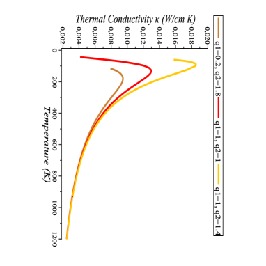
Figure 5: Thermal conductivity $\kappa$ of $Fe$ as a function of temperature in the range of $T=0,\cdots,1200K$, and values for $q_{1}$ and $q_{2}$ given explicitly.

On the left side of the Fig.(4), we have the $Cr_{q-def}$ taking over values: manganese (Mn) when $q_{2}\approx 0.4$, titanium (Ti) with $q_{2}\approx 0.77$ and $Fe$ bulk $q_{2}\approx 0.95$. On the right, we have the behavior of the curves obtained for the electrical conductivity ($\sigma$), where we observe that the ytterbium (Yb) e.g., has its value reached by $Fe_{q-def}$ for $q_{2}\approx 0.7$ and the $Cr_{q-def}$ $q_{2}\approx 0.78$. Notice that in the present case $q_{2}$ develops an effect of impurity of the material. Such that the more $q$ approaches zero the less thermal and electric conductivities approaches zero too. This is in accord with the experimental measures of conductivity of some good conductor that reduces e.g., its electrical conductivity by doping it with impurities.

Let us now return to Eq.(29), where we have the complete Debye function $D(\alpha_{0_{q_{1},q_{2}}})$ to see the behavior of the thermal conductivity. Thus, in the Fig.(5), we show a comparison to the thermal conductivity $\kappa$ for a pure and impure material. We have the thermal conductivity as a function of temperature (T) for $Fe$ (bulk) and a combination of the values $q_{1}$ and $q_{2}$ for the $Fe_{q-def}$ (impure). Therefore, we have the $Fe$ (red) when $q_{1}=q_{2}=1$ (pure), and when $q_{1}=0.2$ and $q_{2}=1.8$, we have a similar behavior to silicon (Si) (golden), whose value for the Debye temperature is $\theta_{D}=645K$. Finally, for a combination of values $q_{1}=1$ and $q_{2}=1.4$ we have a curve that is similar to that of zinc (Zn) (orange), with $\theta_{D}=327K$.

We note that there are a large number of combinations of $q_{1}$ and $q_{2}$ parameter values to be tested. In Tab. (1) we show only two options ($q_{1}=1,q_{2}=0.1$) and ($q_{1}=1,q_{2}=0.5$) and Figs.(3, 4) it is shown that one pure material gets impurities by doping, for instance, it may present properties of other kit2 . The results of this study with two deforming parameters differ from the results previously obtained in bri2 by considering only one parameter. Now is clear there exists another one parameter that can play a different role of the other.

IV Conclusions

We apply the Fibonacci oscillators through the energy spectrum in the Einstein solid and thus expanded to the Debye model, where our results show that the ($q_{1},q_{2}$)-deformed Debye temperature, specific heat, thermal and electrical conductivity of ‘deformed’ chemical elements can assume similar values of other pure elements. The results obtained in our study show that by inserting two deformation parameters $q_{1}$ and $q_{2}$, rather than of a parameter $q$, increases the adjustment range, i.e., we can have different combinations of values as present in Fig. (5). The existence of more degrees of freedom as in the present case of two deformation parameters, $q_{1}$ and $q_{2}$, can be well associated with different types of deformations related to two distinct phenomena of disorders or impurities such as, for instance, one due to pressure generating disorders and other due to doping, respectively.

References

• (1) C. Kittel, Introduction to Solid State Physics, John Wiley & Sons, (1996)
• (2) R.K. Patthria, Statistical Mechanics, Pergamon press, Oxford (1972)
• (3) K. Huang, Statistical Mechanics, John Wiley & Sons, (1987)
• (4) P.W. Anderson, Phys. Rev. 5, 109 (1958).
• (5) P.A. Lee, T.V. Ramakrishnan, Rev. Mod. Phys. 2, 57 (1985).
• (6) Elliott et al., Rev. Mod. Phys. 3, 46 (1974).
• (7) C. Tsallis, J. Stat. Phys. 52, 479 (1988).
• (8) A.A. Marinho, F.A. Brito, C. Chesman, Physica A 391, 3424-3434 (2012).
• (9) D. Tristant, F.A. Brito, Physica A 407, 276-286 (2014).
• (10) A.A. Marinho, F.A. Brito, C. Chesman, J. Phys. Conf. Series 568, 012009 (2014).
• (11) F.H. Jackson, Proc. Edin. Math. Soc. 22, 28-39(1904).
• (12) M. Arik, et al., Z. Phys. C 55, 89-95 (1992).
• (13) A. Algin, Phys. Lett. A 292, 251-255 (2002); A. Algin, B. Deviren, J. Phys. A: Math. Gen. 38, 5945-5956 (2005); A. Algin, J. Stat. Mech. Theor. Exp. P10009, 10 (2008); A. Algin, E. Arslan, J. Phys. A: Math. Theor. 41, 365006 (2008); A. Algin, E. Arslan, Phys. Lett. A 372, 2767-2773 (2008); A. Algin , M. Arik, D. Kocabicakoglu, Int. J. Theor. Phys.47, 1322-1332 (2008); A. Algin, J. Stat. Mech. Theor. Exp. P04007, 04 (2009); A. Algin, J. CNSNS 15, 1372-1377 (2010).
• (14) A.M. Gavrilik, A.P. Rebesh, Mod. Phys. Lett. A 22, 949-960 (2007).
• (15) A.A. Marinho, F.A. Brito, C. Chesman, Physica A 411, 74-79 (2014).
• (16) L. Biedenharn, J. Phys. A: Math. Gen. 22, L873 (1989).
• (17) A. Macfarlane, J. Phys. A: Math. Gen. 22, 4581 (1989).
• (18) J. Fuchs, Affine Lie Algebras and Quantum Groups, Cambridge University Press (1992).
• (19) A. Erzan, Phys. Lett. A 225, 235 (1997).
• (20) A.U. Klimyk, Spectra of Observables in the $q$-Oscillator and $q$-Analogue of the Fourier Transform, Methods and Applications, 1, 8, (2005).
• (21) Daoud M., Kibler M., Phys. Lett A 206, 13-17 (1995).
• (22) Gong R S, Phys. Lett A 199, 81-85 (1995).
• (23) A. Lavagno and N.P. Swamy, Phys. Rev. E 61, 1218 (2000); A. Lavagno and N.P. Swamy, Phys. Rev. E 65, 036101 (2002); A. Lavagno, P.N. Swamy, Found Phys. 40, 814-828 (2010); A. Lavagno, P.N. Swamy, Physica A 389, 993-1001 (2010); A. Lavagno, A. M. Scarfone and P. N. Swamy, J. Phys. A: Math. Theor. 40, 8635-8654 (2007); A. Lavagno, J. Phys. A: Math. Theor. 41, 244014 (2008); A. Lavagno, Int. J. Mod. Phys. B 23, 235-250 (2009); A. Lavagno,G. Gervino, J. Phys. Conf. Series 174, 012071 (2009).
• (24) M. Arik, D.D.Coon, J. Math. Phys. 17, 524 (1976).
• (25) J.M. Ziman, Electron and Phonons - The Theory of Transport Phenomena in Solids, Oxford Univ. Press, (1960).