Stout: Cloudy’s Atomic and Molecular Database

Abstract

We describe a new atomic and molecular database we developed for use in the spectral synthesis code Cloudy. The design of Stout is driven by the data needs of Cloudy, which simulates molecular, atomic, and ionized gas with kinetic temperatures $2.8{\rm\thinspace K}<T<10^{10}~{}{\rm\thinspace K}$ and densities spanning the low to high-density limits. The radiation field between photon energies $10^{-8}$ Ry and 100 MeV is considered, along with all atoms and ions of the lightest 30 elements, and $\sim 10^{2}$ molecules. For ease of maintenance, the data are stored in a format as close as possible to the original data sources. Few data sources include the full range of data we need. We describe how we fill in the gaps in the data or extrapolate rates beyond their tabulated range. We tabulate data sources both for the atomic spectroscopic parameters and for collision data for the next release of Cloudy. This is not intended as a review of the current status of atomic data, but rather a description of the features of the database which we will build upon.

1 Introduction

Cloudy is an openly available spectral simulation code based on detailed microphysics, most recently reviewed by Ferland et al. (2013a). It considers microphysical processes from first principles to determine the excitation, ionization, and thermal properties of a mix of gas and dust. Much of this physics is described in Osterbrock & Ferland (2006), hereafter AGN3. A very wide range of densities and temperatures can be modeled, and the full radiation between $10^{-8}$ Ry and 100 MeV is considered.

Massive amounts of atomic and molecular data are needed to do such simulations. These include energy levels; transition probabilities; collision rates with electrons, protons, and atoms; photoionization cross sections; collisional ionization rate coefficients; recombination rate coefficients, along with charge exchange ionization/recombination data. There are several spectral databases available, including Chianti (Dere et al., 1997; Landi et al., 2012) LAMDA (Schöier et al., 2005), JPL (Pickett et al., 1998), and CDMS (Müller et al., 2001, 2005). These provide energy levels, and transition probabilities. Chianti and LAMDA also include collision rates with a particular emphasis on certain applications. Chianti and LAMDA are included in the Cloudy distribution and are used in our simulations (Ferland et al., 2013a; Lykins et al., 2013).

At times during the development of Cloudy, we have need to create additional models of atoms or molecules. What format should we use? Chianti comes closest to providing the data we need, but its format does not allow for more than 999 levels and the collision rates are presented in a format that is far removed from the original published form. Only a few spline points are given for collision rates, and they emphasize temperatures higher than those found in photoionization equilibrium, so the fits are sometimes not valid at the low temperatures we need (Ercolano et al., 2008). Chianti’s use of spline interpolation can lead to unphysical negative collision strengths in Chianti version 7. Furthermore, we must include collisions with atoms and molecules, which are important for photodissociation regions (PDR) calculations. Hence the need for our own database.

This paper describes how we implemented our spectral line database. It is not intended as a definitive reference for the state of the art in atomic and molecular data today. Continuous updates to the database will occur and be described in future papers.

2 The Stout Database

The new database was designed to have the following properties:

• The data format must be easy for a person to maintain since continual updating is necessary.

• It must provide for different types of data. For example, radiative rates might be specified as oscillator strengths, transition probabilities, or line strengths.

• Collision data should, if possible, cover the temperature range considered by Cloudy, currently 2.8 K to 10¹⁰ K. This is seldom available so we need to have a strategy to extrapolate beyond the limits of the tabulated data.

• We must be able to reliably interpolate upon tables of rate coefficients without producing unphysical negative values, which may introduce negative collision rates.

• Both resonance and subordinate lines must be included since Cloudy is applied to dense environments where subordinate lines are important.

• Both molecular and atomic data must be considered.

• A broad range of collision partners, including electrons, H₂, H⁰, He, and H⁺, must be considered.

• Each file must explain its provenance by documentation at the end of the file.

• As far as possible, the data must be presented in their original format. We use the tabulated collision rates, collision strengths, energies, etc, as they appear in the original publication. This makes the data much easier to maintain.

• Numbers within data files are free format. Each number need only be surrounded by a space or tab character to distinguish separate entries. This makes it both easier to maintain and to remain close to the format of the original data source.

• There must be no limit to the number of levels in a model.

2.1 Spectral models in Cloudy

We begin with a description of the atomic models in Cloudy. Cloudy has two distinctly different types of atomic models due to the different level structures of various isoelectronic sequences (Ferland et al., 2013a). The H- and He-like isoelectronic sequences have excited states that are closer to the continuum than the ground state. As a result, these states are strongly coupled to the continuum, with levels populated following recombination or collisions between excited states or the continuum. Excited states are relatively weakly coupling to the ground state. The H- and He-like isoelectronic sequences use the models described by the series of papers starting with Bauman et al. (2005) and Porter et al. (2005). Porter et al. (2009, 2012, 2013) give the most recent updates.

For more complex ions, the lowest excited states are close to the ground state and are strongly coupled to it. The influence of the continuum is weak. The remaining atoms and ions are treated with the atomic models described in this paper or with Chianti. The Appendix contains Table 5 that summarizes the data sources we use. We describe how we use these data in the following subsections.

The data for the atomic species, contained in the Stout database, are located in separate directories for each species with a structure similar to that of Chianti. Each data set consists of three files - energy levels (the file with the extension “nrg”), transition probabilities (extension “tp”), and collision data (extension “coll”).

2.2 Energy levels

We use the experimental level energies from NIST (Kramida et al., 2014) if possible. Experimental data are available for most species. The level energies given in the NIST database are usually derived from measured line wavelengths. If there are no experimental data, we utilize theoretical data which often are of lower accuracy.

Transition rates that come from theoretical calculations must be corrected for any differences between experimental and theoretical energies. The level ordering may not agree so it is absolutely important to match the level assignments given in different data sources. When this issue is overcome, the integrity of the particular system is assured, and the calculated collisional parameters and radiative parameters are consistent with the experimental energy levels.

By default we report wavelengths, in Ångström that are derived from the stored energy levels (so-called Ritz wavelengths). We do allow the wavelength to be specified to override this default. The convention in atomic physics is to use air wavelengths for $\lambda>2000$ Å and vacuum wavelengths for $\lambda<2000$ Å. More recently, work has started to appear which uses vacuum for all wavelengths. The Sloan project (see The Sloan Digital Sky Survey at http://www.sdss.org) is an example. By default we follow the atomic physics convention but provide an option to report only vacuum wavelengths. The index of refraction of air is taken from Peck & Reeder (1972).

Table 1: A sample of the level energies file (s_2.nrg) for S II from Stout. The first column represents the level index that is used in the transition probability and collision data files, the second column gives level energies (in cm^-1), the third column gives level statistical weights $g$, and the last two columns give a level designation with “*” standing for odd-parity levels.

We present a sample of a file with columns description for the energy level data in Stout in Table 1. Just a small part of the file s_2.nrg with the S II ion level energies are given here. The complete data table is given by Kisielius et al. (2014a), whereas level data are taken from the NIST database (Kramida et al., 2014). Only the level numbers, energies, and the statistical weights are utilized for deriving of the transition probability or collision strengths, whereas the configuration and $LS\pi$ are given for information purposes.

2.3 Radiative transitions

The radiative transition between the upper level $u$ and the lower level $l$ can be parameterized as a line strength $S$, oscillator strength $f$ (or $gf$), or transition probability $A$, although only the latter enters in a calculation of level populations and emission spectra. Different data sources will provide different parameters, and we accept all three.

We prefer to utilize the transition line strength $S$ over the weighted oscillator strengths $gf$ or transition probabilities $A$. The advantage to $S$ is that it does not depend explicitly on the transition energy $\Delta E$ (or the transition wavelength $\lambda$), whereas $gf$ and $A$ do. Many published transition data are the result of theoretical calculations and use theoretical energies while we use experimental energies where possible. Therefore, a correction due to the uncertainty in the calculated transition energy $\Delta E$, or wavelength $\lambda$, values must be done. The conversion to the experimental transition energies $\Delta E_{\mathrm{exp}}$ or observed transition wavelengths $\lambda_{\mathrm{exp}}$ is:

$$A_{\mathrm{corr}}^{k}=A_{\mathrm{th}}^{k}(\Delta E_{\mathrm{exp}}/\Delta E_{\mathrm{th}})^{2k+1}=A_{\mathrm{th}}^{k}(\lambda_{\mathrm{th}}/\lambda_{\mathrm{exp}})^{2k+1}$$ (1)

where $k$ is the transition multipole order ($k=1,2,3,...$), $A$ is the transition probability, $\lambda_{\mathrm{th}}$ is the theoretical transition wavelength.

Table 2: Conversion factors and coefficients from the transition line strengths $S$ (in a.u.) to the radiative transition probabilities $A$ (in s^-1).

type	factor $C_{\lambda}$	$C_{\lambda}$	$C_{\Delta E}$
$E1$	$\frac{64\pi^{4}e^{2}a_{0}^{2}}{3h}$	$2.02613\times 10^{18}$	$2.14200\times 10^{10}$
$M1$	$\frac{64\pi^{4}\mu_{\mathrm{B}}^{2}}{3h}$	$2.69735\times 10^{13}$	$2.85161\times 10^{5}$
$E2$	$\frac{64\pi^{6}e^{2}a_{0}^{4}}{15h}$	$1.11995\times 10^{18}$	$5.70322\times 10^{4}$
$M2$	$\frac{64\pi^{6}\mu_{\mathrm{B}}^{2}a_{0}^{2}}{15h}$	$1.49097\times 10^{13}$	$7.59260\times 10^{-1}$
$E3$	$\frac{2048\pi^{8}e^{2}a_{0}^{6}}{4725h}$	$3.14441\times 10^{17}$	$7.71311\times 10^{-2}$
$M3$	$\frac{2048\pi^{8}\mu_{\mathrm{B}}^{2}a_{0}^{4}}{4725h}$	$4.18610\times 10^{12}$	$1.02683\times 10^{-6}$

The transition line strength $S$ is expressed in atomic units (a.u.). It is symmetric in relation to the initial and final states, and is obtained as a square of the corresponding $E1$, $M1$, $E2$, $M2$, $E3$, $M3$ transition matrix elements. In this case, the electric multipole emission transition probability (Einstein $A$-coefficient) $A_{ul}^{k}$ (in s^-1) can be determined as

$$A_{ul}^{k}=C_{\lambda}S/(g_{u}\lambda^{2k+1})$$ (2)

where $g_{u}$ is the statistical weight of the upper level, and $C_{\lambda}$ is the conversion factor. The expressions of the factor $C_{\lambda}$ for various multipole transitions are presented in Table 2. We provide numerical values of the conversion coefficients when $\lambda$ is expressed in Å and the line strength $S$ is calculated in a.u. In the case when we have the transition energy $\Delta E$ instead of wavelength, we can use similar expression for $A_{ul}^{k}$:

$$A_{ul}^{k}=C_{\Delta E}(\Delta E)^{2k+1}S/g_{u}.$$ (3)

The conversion coefficients $C_{\Delta E}$ are given in Table 2 for $\Delta E$ determined in a.u. For different energy units, one must rely on these standard relations: 1 a.u.$=2$ Ry$=27.211385$ eV$=219474.63$ cm^-1, and the inverse relations: 1 Ry$=0.5$ a.u.; 1 eV$=0.036749324$ a.u.; 1 cm${}^{-1}=4.5563353\cdot 10^{-6}$ a.u. Having the radiative transition probabilities of various multipole orders, one can simply derive the absorption oscillator strengths $f_{lu}$ using a simple expression:

$$f_{lu}=1.4992\times 10^{-16}\lambda^{2}(g_{u}/g_{l})A_{ul}$$ (4)

where $g_{l}$ is the statistical weight of the lower level. The relation between the oscillator strength $f$ and transition probability $A$ does not depend on the radiative transition type.

Table 3: A sample of the transition probabilities file (s_2.tp) for S II from Stout. The first column represents radiative transition data type (“A” for a transition probability, “f” for weighted oscillator strength, “S” for a line strength), the second column gives the lower level index, the third column gives the upper level index, the fourth column gives a transition parameter value, and the final column points to the radiative transition type ($E1$, $E2$, $E3$, …, $M1$, $M2$, …).

Table 3 gives a sample of the transition data file for S II, with the data coming from Kisielius et al. (2014a). The transition line strengths $S$ are given as the basic radiative transition data as they do not depend explicitly on the transition energy. The NIST database traditionally provides the radiative transition probabilities (rates) $A$. Conversion from the transition line strengths $S$ to the transition probabilities $A$ depends on the transition type. It can be performed with the help of Table 2.

2.4 Collisions

Collisional data can be given as collision strengths, effective collision strengths, collision cross sections, and rate coefficients. In the electron-impact excitation:

$$\mathrm{A}^{N+}(E_{l})+e(\varepsilon_{l})\rightarrow\mathrm{A}^{N+}(E_{u})+e(\varepsilon_{u}),$$ (5)

the energy conservation law leads to

$$E_{l}+\varepsilon_{l}=E_{u}+\varepsilon_{u}.$$ (6)

Here $E_{l}$ and $E_{u}$ are the energies of the lower and upper levels, $\varepsilon_{l}$ and $\varepsilon_{u}$ are the kinetic energies of the incident and the scattered electron.

Maxwellian-averaged effective collision strengths are utilized in Stout. Here we provide the basic relations for these parameters, whereas data sources are given in Table 5. Our preferred method is to use collision data calculated in the close-coupling (CC) approach, e.g., the R-matrix method. Unfortunately, such data are not available for many ions. Even in the case when some data exist, these usually deal with only a few of the lowest levels or even the $LS$ terms with unresolved fine-structure levels. So one must resort to less elaborate approaches, such as the distorted-wave method, the plane-wave approximation, or a $\bar{g}$ (g-bar) formula, for the remaining data.

The dimensionless collision strength $\Omega$ is the best to describe the electron-impact excitation process from the lower level $E_{l}$ to the excited level $E_{u}$. It is symmetrical in regard to the initial and final states parameter, i.e, $\Omega_{lu}=\Omega_{ul}$. For ions, it has a finite value at the excitation threshold and varies only slightly with the incident electron energy if autoionization resonances are not considered. For neutral atoms, the collision strength $\Omega_{lu}$ goes to zero at the excitation threshold.

At high incident electron energies, the behavior of the collision strength depends on the transition (line) type and has a different form for allowed or forbidden transitions. The collision strength $\Omega_{lu}$ is determined as a square of the excitation operator’s matrix element. It is connected to the excitation cross-section $\sigma_{lu}$ and the de-excitation cross-section $\sigma_{ul}$ by simple relations:

$$\sigma_{lu}(\varepsilon_{l})=\Omega_{lu}\frac{\pi\mathrm{a}_{0}^{2}}{g_{l}E_{l}}$$ (7)

and

$$\sigma_{ul}(\varepsilon_{u})=\Omega_{ul}\frac{\pi\mathrm{a}_{0}^{2}}{g_{u}E_{u}},$$ (8)

where $\pi\mathrm{a}_{0}^{2}=8.7972\times 10^{-17}$ cm²  is the atomic cross-section unit. For electric dipole allowed transitions, one can express the excitation cross section $\sigma_{lu}$ through an effective Gaunt factor ${\bar{g}}_{lu}(\varepsilon_{l})$ (as in Mewe, 1972), often called the “g-bar approximation”:

$$\sigma_{lu}(\varepsilon_{l})=\frac{8\pi f_{lu}{\bar{g}}_{lu}(\varepsilon_{l})}{\sqrt{3}\varepsilon_{l}(E_{u}-E_{l})}$$ (9)

with $f_{lu}$ being the absorption oscillator strength.

The collision strengths are integrated over a Maxwellian distribution of free-electron energies in order to determine the effective collision strengths $\Upsilon_{lu}$ = $\Upsilon_{ul}$ (or rate parameters) at some electron temperature $T_{e}$:

$$\Upsilon_{lu}=\int_{0}^{\infty}\Omega_{lu}(\varepsilon_{u})\exp(-\varepsilon_{u}/k_{\mathrm{B}}T_{e})d(-\varepsilon_{u}/k_{\mathrm{B}}T_{e}).$$ (10)

Here $k_{\mathrm{B}}$ refers to Boltzmann’s constant. In this case, the excitation rate coefficient $q_{lu}$ (in cm³ s^-1) is expressed as

$$q_{lu}=8.629\times 10^{-6}\frac{\exp((E_{l}-E_{u})/k_{\mathrm{B}}T_{e})\Upsilon_{lu}}{{\rm\thinspace g}_{l}T_{e}^{1/2}},$$ (11)

whereas the de-excitation rate coefficient $q_{lu}$ is determined by formula:

$$q_{ul}=8.629\times 10^{-6}\frac{\Upsilon_{lu}}{{\rm\thinspace g}_{u}T_{e}^{1/2}}.$$ (12)

Table 4: A fragment of the effective collision strength file s_2.coll for the ion S II from Stout. The first column represents data type, e.g., “TEMP” stands for a temperature grid (in  K), “CSELECTRON” for the effective electron-impact excitation strength $\Upsilon$, “RATE PROTON” for the proton excitation rate, etc. The data types and their sources are provided in the same file in the comments lines. The second column gives the lower level index, the third column gives the upper level index, and next columns give a particular collision parameter for the corresponding temperature.

Table 4 gives a fragment of the collision data file s_2.coll for S II. For this ion we employ the electron-impact excitation data from Tayal & Zatsarinny (2010). There can be several temperature grids in one data file, especially when different projectiles, such as electrons, protons, hydrogen atoms, or hydrogen molecules, are described. In a similar way, there can be different data sources for different level combinations even for the same collider. The collision data for a given transition and collider will be overwritten if new data for that transition and collider appear later in the file when read in by Cloudy.

Most of the data sources in Table 5 are given for the electron collisions. Nevertheless, some colliders other than electrons are included. For an atomic hydrogen collider, very important in PDRs, we use data from Launay & Roueff (1977) for C I, from Abrahamsson et al. (2007); Krems et al. (2006) for O I, from Hollenbach & McKee (1989) for Ne II, from Barklem et al. (2012) for Mg I, and from Barinovs et al. (2005) for Si II. For proton colliders, very important in collisions between levels with similar energies, we utilize data from Roueff & Le Bourlot (1990) for C I and data from Pequignot (1990) for O I. For H₂, data from Schröder et al. (1991) are employed for C I, data from Wiesenfeld & Goldsmith (2013) for the C II ion, and data from Jaquet et al. (1992) for O I. For helium impact on neutrals, we use data from Staemmler & Flower (1991) for C I, and from Monteiro & Flower (1987) for O I.

For collisions involving molecules, the literature often gives deexcitation rates rather than collision strengths. We accept deexcitation rates for any transition and species.

It is necessary to interpolate within tables of collision rates versus temperature, and in many calculations, extrapolate beyond the tabulated range. Within the table, we interpolate using the method of Fritsch & Butland (1984), which is local and piecewise cubic, and maintains the monotonicity properties of the underlying data. This ensures that the interpolation does not introduce any “overshoots”, where the interpolated value does not lie within the range of the tabulated data. Such overshoots appear to be the source of the negative collision strengths that are present in version 7 of the Chianti database.

2.4.1 Temperature extrapolation for atoms and ions

Cloudy considers the temperature range extending from 2.8 K to 10¹⁰ K and considers all ions of the first thirty elements along with several dozen molecules. Gaps in the collision data are common. Often we must extrapolate beyond the range of the tabulated data, or improvise entire collections of data.

For temperatures below the range of the tabulated data, and for ions with positive charge, we assume that the collision strength is constant to extrapolate below the lowest tabulated temperature. Physically, an effective collision strength is a Boltzmann average over the excitation cross section. As the temperature goes to zero, this average is over a narrow range near threshold, and will tend to be constant. This is not true if there are strong resonances very near threshold but it is a reasonable first approximation. For neutral species the collision strength goes to zero at energies near threshold so the effective collision strength also goes to zero as $T\rightarrow 0$. We do a linear interpolation between the lowest temperature value and 0.0. We use these collision strength laws to form the appropriate temperature scaling when working with data giving collisional deexcitation rates.

For high temperatures we use Burgess & Tully (1992) to guide the extrapolation. Burgess & Tully (1992) consider three possible types of transitions with different behavior at high energies (temperatures), Type 1 for the electric dipole transitions, Type 2 for the non-electric dipole, non-exchange transitions, Type 3 for the exchange transitions, with Types 4 and 5 being special cases (for more details on the transition classification see Burgess & Tully (1992)). We use the first two types, Type 1 and Type 2. The Type 3 classification can be avoided when levels and transitions are expressed in the intermediate coupling rather than pure $LS$ coupling. In this case one can not separate the spin-changing transitions since the selection rules are applied for the total angular momentum $J$.

Transition types can be deduced from the energy levels files (*.nrg) where $J$, configurations and their parities are given or from the radiative transition files (*.tp) where transition types are given (but these are not present in all transition data files). In general, our data files contain information necessary to make a separation between Type 1 and Type 2 transitions. For the Type 1 transitions, the high-temperature behavior of the effective collision strength $\Upsilon$ is described by a simple relation $\Upsilon=C_{1}\ln(T_{e})$. The value of $C_{1}$ can be derived from the last tabulated temperature point in the data file. For the Type 2 transitions, the effective collision strength does not depend on the electron temperature $T_{e}$, i.e., $\Upsilon=C_{2}$. The value of $C_{2}$ is the value of $\Upsilon$ at the last tabulated temperature.

Tests show that the low-temperature extrapolation does affect calculations. In photoionization equilibrium very low kinetic temperatures are possible (Osterbrock & Ferland, 2006). The constant temperature test cases in the Leiden PDR comparison (Röllig et al., 2007) have $T_{\mathrm{kin}}=50{\rm\thinspace K}$, lower than many tabulated rates. Predictions of some Leiden test cases were affected by the form of the low-$T$ extrapolation.

2.4.2 Gaps in the collision data

We use the $\bar{g}$ approximation (Seaton, 1962; van Regemorter, 1962) to fill in missing electron collision data. This is a highly approximate relationship between the transition probability or oscillator strength, and the collision strength. We use Mewe (1972) for those isoelectronic sequences he considered, and van Regemorter (1962) for others.

We provide a way to test the effects of such uncertain data. Cloudy includes a built-in Gaussian random noise generator. This was used, for instance, to assay the effects of missing H₂ collision rates upon the final spectrum (Shaw et al., 2005). Repeated calculations will reveal the uncertainties introduced by the approximations, if the uncertainties can be quantified.

Some databases have no radiative transition between large blocks of levels. For instance, a species may have no E1 transitions between the ground and first excited configurations. Higher order transitions are possible but many databases present only E1 transitions. If theoretical collisional rates have not been computed, then there would not be any coupling between the configurations. It is not possible to simultaneously solve for the populations; the matrix becomes ill conditioned. In cases where we have no radiative or collision data, we leave the radiative transition rate as zero and use an electron effective collision strength of $10^{-10}$ . This was chosen to be as small as possible while allowing the linear algebra to function properly.

2.4.3 Temperature extrapolation for molecular excitation

When molecular collisional deexcitation rate coefficients $q(T)$ are provided only over a limited temperature range, the following two simple extrapolation approaches are applied:

$$q(T)=q(T_{\rm low}),~{}~{}~{}~{}~{}~{}T<T_{\rm low},$$ (13)

and

$$q(T)=q(T_{\rm high})\left({{T}\over{T_{\rm high}}}\right)^{1/2}\exp(-T/10^{5}{~{}\rm K}),~{}~{}~{}~{}~{}T>T_{\rm high}.$$ (14)

$T_{\rm low}$ and $T_{\rm high}$ correspond to the low and high temperature limit, respectively, of the data. The extrapolation formulae are valid for inelastic collisions of neutral molecules (e.g., OH) or molecular ions (e.g., HCO⁺) with neutral colliders (e.g., H, He, H₂) for deexcitation (downward) transitions resulting in changes in fine-structure, rotational, and/or vibrational levels of the target molecules. Physical justifications for the extrapolations as well as caveats for their use are described below.

Extrapolation to low temperature

The deexcitation rate coefficients as a function of temperature $T$ are obtained by thermally averaging the inelastic integral cross sections over a Maxwellian kinetic energy distribution given by

$$q_{u\rightarrow l}(T)=\left(\frac{8k_{\mathrm{B}}T}{\pi\mu}\right)^{1/2}\frac{1}{(k_{\mathrm{B}}T)^{2}}\int_{0}^{\infty}\sigma_{u\rightarrow l}(E_{\mathrm{kin}})\exp(-E_{\mathrm{kin}}/k_{\mathrm{B}}T)E_{\mathrm{kin}}dE_{\mathrm{kin}},$$ (15)

where $\sigma_{u\rightarrow l}(E_{\mathrm{kin}})$ is the state-to-state inelastic cross section, $E_{\mathrm{kin}}$ the center of mass kinetic energy, $\mu$ the reduced mass of the collision complex, and $l$ ($u$) the lower (upper) levels in the molecule.

Rewriting Eq. (15) with the cross section in terms of the relative velocity $v$ of the collision system gives (Flower, 1990)

$$q_{u\rightarrow l}(T)=\left(\frac{2}{\pi}\right)^{1/2}\left(\frac{\mu}{k_{\mathrm{B}}T}\right)^{3/2}\int_{0}^{\infty}\sigma_{u\rightarrow l}(v)\exp(-\mu v^{2}/2k_{\mathrm{B}}T)v^{3}dv.$$ (16)

If the cross section is assumed to have the analytical form

$$\sigma_{u\rightarrow l}(v)=Bv^{a},$$ (17)

for all $v$ (or $E_{\mathrm{kin}}$) where $B$ is an (undetermined) constant and $a$ is some power, then the rate coefficient takes the form

$$q(T)=A(a)B(T/\mu)^{b}$$ (18)

(Walker et al., 2014). Here $b=(a+1)/2$ and $A$ is a function of $a$, both deduced from the Gaussian integral in Eq. (16). This result is exact, given the assumption of Eq. (17), and applicable to all collision systems. It is approximate if the cross section dependence varies with $v$ as in real systems.

Now at sufficiently low kinetic energy, Wigner (1948) showed that the inelastic cross section takes the form

$$\sigma_{u\rightarrow l}\sim E^{\ell-1/2}_{\mathrm{kin}},$$ (19)

where $\ell$ is the total orbital angular momentum of the collision complex. In most systems of interest, $s$-wave scattering (i.e., $\ell=0$) is allowed and dominates at low kinetic energy. Therefore,

$$\sigma_{u\rightarrow l}\sim E^{-1/2}_{\mathrm{kin}}\sim v^{-1},$$ (20)

or $a=-1$, $b=0$ and the rate coefficient becomes a constant, independent of temperature as given by Eq. (13).

Equation (13) is absolutely valid under two conditions: i) when $T<T_{\rm Wigner}$, the so-called Wigner regime, where higher partial waves ($\ell>0$) do not contribute to the cross section and ii) when relevant selection rules do not forbid $s$-wave scattering. Typically, $T_{\rm Wigner}\sim$ mK and much less than $T_{\rm low}$. However, for $T\sim 1-100$ K the rate coefficient is usually oscillatory due to the presence of orbiting and Feshbach resonances in the cross section. This behavior cannot be easily analytically reproduced so that extrapolating the Wigner threshold behavior of Eq. (20) to $T_{\rm low}$ is a reasonable pragmatic approach.

In the event that $s$-wave scattering is forbidden for the particular transition (which is rare), the cross section would drop rapidly to zero as $v$ goes to zero

$$\sigma_{u\rightarrow l}\sim E^{1/2}_{\mathrm{kin}}\sim v.$$ (21)

The rate coefficient would be overestimated by Eq. (13), but this error would be limited to low astrophysical temperatures, $T\mathrel{\hbox{\hbox to0.0pt{\hbox{\lower 4.0pt\hbox{$\sim$}}\hss}\hbox{$<$}}}$ 10 K.

Extrapolation to High Temperature

A number of approaches have been proposed for extrapolating the deexcitation rate coefficient to higher temperatures beyond $T_{\rm high}$. For linear molecules, Schöier et al. (2005) fitted the available data in LAMDA to the form

$$q(T)={{\alpha}\over{k_{\mathrm{B}}}T}\exp(-\beta/(k_{\mathrm{B}}T)^{1/4})\exp(-\gamma/(k_{\mathrm{B}}T)^{1/2})$$ (22)

where $\alpha$, $\beta$, and $\gamma$ are fit parameters and then used the fit for $T>T_{\rm high}$. A more pragmatic approach, which avoids fitting, is to apply a hard-sphere model. This assumes that the cross section is independent of kinetic energy giving $a=0$ and $b=1$ in Eqs. (17) and (18), respectively, so that

$$q(T)\sim T^{1/2}.$$ (23)

However, the inelastic cross section typically turns up to a maximum near a few eV before decaying at higher energies due to the increasing importance of collisional dissociation, electronic excitation, and collisional ionization. Therefore, to prevent the rate coefficient from growing too large at high $T$, the relation (23) is multiplied by an exponential damping factor to give Eq. (14). The exact form is not important as the molecular abundances decrease rapidly for $T\gtrsim 5000$ K.

3 Other details

3.1 Baseline models, unmodelled species

Many species have level energies and transition probabilities tabulated in NIST, but have no electron collisional rates at all. For these species we created “baseline” Stout data files. These contain the NIST level energies and transition probabilities but use the $\bar{g}$ approximation for all collision data. These are marked as “baseline” in Table 5.

It was not possible to create models for all ions. NIST did not have sufficient data to compute models for the following species: F I, Cl XIII, Cl XV, Sc I, Ti I, Ti II, V I, V II, V III, V V, V XIV, Cr I, Cr III, Cr V, Mn II, Mn III, Mn IV, Mn VII, Co I, Co IV, Co V, Co VI, Co VII, Co IX, Ni VI, Ni VIII, Ni X, Cu II, Cu III, Cu IV, Cu V, Cu VI, Cu VII, Cu VIII, Cu IX, Cu X, Cu XII, Cu XII, Cu XIX, Cu XX, Zn I, Zn III, from Zn V to Zn XIX, and Zn XXI, Zn XXII, Zn XXVI. As a result Cloudy calculations do not predict lines of these ions. Calculating sufficient data for these species should be a high priority.

3.2 Masterlists - specifying which database

Cloudy uses a total of three databases, Stout, described here, along with Chianti and LAMDA. Each database has its own “masterlist”, a file specifying the species present in that version of the database. The Stout masterlist file was used to derive Table 5.

In a particular Cloudy calculation, each of these masterlist files will be read. It is likely that a particular species is present in more than one database and its masterlist file. The priorities for deciding which database to use are: 1) the H- and He-like isoelectronic sequences are always treated with our unified model, 2) Stout, 3) Chianti, and 4) LAMDA.

3.3 Suprathermal electrons

When cosmic rays or Auger electrons enter neutral gas they create a population of suprathermal electrons which ionize and excite the gas (Spitzer & Tomasko, 1968). We solve for the population of these suprathermal electrons explicitly.

These electrons have an energy of typically 20 - 40 eV and can cause internal excitations of all atoms and molecules. We include this as a general excitation process using the Born approximation outlined by Shemansky et al. (1985).

4 Discussion and Summary

As described in the mandate for the development of Stout, it is now far easier to maintain and update the line database in Cloudy, and to add entirely new species. With the addition of the species given in Table 5 there are now far more lines predicted than in previous versions of the code, producing far richer spectra.

Figure 1 shows an example. This is a coronal equilibrium metal-rich ($Z=35Z_{\sun}$) gas with a density of 1 cm^-3 and a temperature of $5\times 10^{4}{\rm\thinspace K}$. The panels compare the current version, soon to be released as C15, with C10, the last Cloudy release before beginning the move of ionic models to external databases. There are now a far greater number of faint lines.

Despite the large increase in the number of lines the total cooling of the gas is relatively unaffected. Lykins et al. (2013) describe our calculation of the total gas cooling along with our strategy for determining how many levels to model. The cooling is dominated by a few very strong lines so the large number of faint lines do not increase it significantly. The faint lines can be important when abundances are non-solar (as in Figure 1), low-abundant species are of interest, or if a number of faint lines blend to produce a stronger feature.

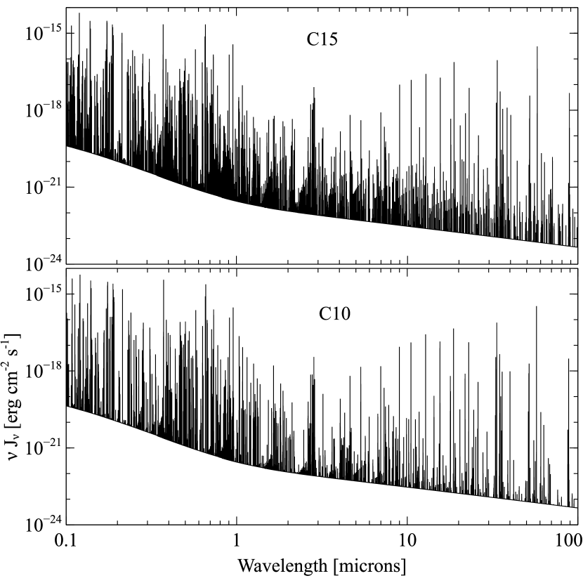
Figure 1: The predicted spectrum of a $Z=35Z_{\sun}$ collisional gas with a temperature of $5\times 10^{4}{\rm\thinspace K}$. The upper panel shows the current results, for C15, while the lower panel is for C10, the last version before the move to external databases for ions. The density of lines is now far greater.

This paper is a definition of our database and explains how Cloudy uses it. It is not intended as a review of the state of the art of atomic data in 2015. Future papers will expand the atomic/molecular data using the framework outlined here.

The database is designed to be easy to maintain and modify due to the need to constantly modify it as new data appear. The format follows the original data papers as closely as possible.

The methods we developed to fill in missing data are described. The data needs of Cloudy are vast due to its very wide range of applicability. We frequently encounter cases where collisional rates are not available at all, or we need to extrapolate beyond the range of computed data. The $\bar{g}$ approximation is used to provide missing electron collision data. This approximation has a very broad dispersion and we provide a method of checking on its impact on predictions. When rates or collision strengths are available, but we need to extrapolate beyond the range of tabulated temperatures, we use physically motivated asymptotic limits. Tests show that predictions are mainly affected by the form of the low-$T$ extrapolation.

The Stout database is part of the Cloudy distribution, available on www.nublado.org. Its version number is the same as the Cloudy version number. This paper is the defining documentation of Stout and should be cited if the database is used outside of Cloudy.

Appendix A Data sources

This Appendix describes the data sources currently used by the development version of Cloudy. Species that are not explicitly listed in this Appendix use the Chianti database. With the combination of these data, Chianti, and our special treatments of the H and He-like iso-electronic sequences, Cloudy includes spectral models of all ions of the lightest thirty elements.

Table 5: Atomic data sources in Stout

$Z$	Species	Data Source
3	Li i	baseline - see text
4	Be i	baseline
	Be ii	baseline
5	B i	baseline
	B ii	baseline
	B iii	baseline
6	C i	Johnson et al. (1987), Mendoza (1983),
		Launay & Roueff (1977),
		Roueff & Le Bourlot (1990),
		Schröder et al. (1991), Staemmler & Flower (1991)
	C ii	Tayal (2008), Wiesenfeld & Goldsmith (2013),
		Goldsmith et al. (2012)
	C iii	Berrington et al. (1985)
7	N i	Fischer & Tachiev (2004), Tayal (2000)
	N v	Liang & Badnell (2011)
8	O i	Bell et al. (1998), Wang & McConkey (1992),
		Barklem (2007), Abrahamsson et al. (2007),
		Krems et al. (2006), Monteiro & Flower (1987),
		Jaquet et al. (1992), Pequignot (1990)
	O ii	Kisielius et al. (2009), Fischer & Tachiev (2004)
9	F i	baseline
	F ii	Butler & Zeippen (1994)
	F iii	baseline
	F iv	Lennon & Burke (1994)
	F v	baseline
	F vi	baseline
	F vii	baseline
10	Ne i	baseline
	Ne ii	Griffin et al. (2001), Hollenbach & McKee (1989)
11	Na i	Verner private communication
	Na ii	baseline
12	Mg i	Barklem et al. (2012), Leep & Gallagher (1976),
		Mendoza (1983)
	Mg iii	Liang & Badnell (2010)
13	Al i	baseline
	Al iii	Dufton & Kingston (1987),
		Sampson et al. (1990)
	Al iv	baseline
	Al vi	Butler & Zeippen (1994)
14	Si i	Hollenbach & McKee (1989)
	Si ii	Tayal (2008), Dufton & Kingston (1994),
		Barinovs et al. (2005)
	Si iii	Dufton & Kingston (1989),
		Callegari & Trigueiros (1998),
		Dufton et al. (1983)
	Si iv	Liang et al. (2009)
	Si vii	Butler & Zeippen (1994)
	Si ix	Lennon & Burke (1994)
15	P i	baseline
	P ii	Krueger & Czyzak (1970)
	P iii	Krueger & Czyzak (1970)
	P iv	baseline
	P vi	baseline
16	S i	Hollenbach & McKee (1989)
	S ii	Kisielius et al. (2014a),
		Tayal & Zatsarinny (2010)
	S iii	Hudson et al. (2012b)
17	Cl i	Hollenbach & McKee (1989)
	Cl v	baseline
	Cl vi	baseline
	Cl vii	Liang et al. (2009)
	Cl viii	Liang & Badnell (2010)
	Cl ix	Berrington et al. (1998)
18	Ar i	baseline
	Ar ii	Pelan & Berrington (1995)
	Ar iii	Galavis et al. (1995)
	Ar iv	Ramsbottom et al. (1997)
	Ar v	Galavis et al. (1995)
	Ar vi	Saraph & Storey (1996)
19	K i	baseline
	K ii	baseline
	K iii	Pelan & Berrington (1995)
	K iv	Galavis et al. (1995)
	K vii	Saraph & Storey (1996)
	K viii	baseline
	K x	baseline
20	Ca i	baseline
	Ca iii	baseline
	Ca iv	Pelan & Berrington (1995)
	Ca vi	baseline
21	Sc i	baseline
	Sc ii	Wasson et al. (2011)
	Sc iii	baseline
	Sc iv	baseline
	Sc v	Pelan & Berrington (1995)
	Sc vi	baseline
	Sc vii	baseline
	Sc viii	baseline
	Sc ix	baseline
	Sc ix	baseline
	Sc x	baseline
	Sc xi	baseline
	Sc xii	baseline
	Sc xiii	Saraph & Tully (1994)
	Sc xiv	baseline
	Sc xv	baseline
	Sc xvi	baseline
	Sc xvii	baseline
	Sc xviii	baseline
22	Ti iii	baseline
	Ti iv	baseline
	Ti v	baseline
	Ti vi	Pelan & Berrington (1995)
	Ti vii	baseline
	Ti viii	baseline
	Ti ix	baseline
	Ti x	baseline
	Ti xiii	baseline
23	V iv	baseline
	V vi	baseline
	V vii	Pelan & Berrington (1995)
	V viii	baseline
	V ix	baseline
	V x	baseline
	V xi	baseline
	V xii	baseline
	V xiii	baseline
	V xv	Berrington et al. (1998)
	V xvi	baseline
	V xvii	baseline
	V xviii	baseline
	V xix	baseline
	V xx	baseline
	V xxi	baseline
24	Cr ii	Grieve & Ramsbottom (2012)
	Cr iii	baseline
	Cr iv	baseline
	Cr v	baseline
	Cr x	baseline
	Cr xi	baseline
	Cr xii	baseline
	Cr xv	baseline
25	Mn i	baseline
	Mn v	baseline
	Mn vi	baseline
	Mn xi	baseline
	Mn xii	baseline
	Mn xiii	baseline
	Mn xiv	baseline
	Mn xvi	baseline
26	Fe i	Hollenbach & McKee (1989)
	Fe ii	Verner et al. (1999)
	Fe iii	Zhang (1996), Kurucz (2009)
	Fe vii	Witthoeft & Badnell (2008)
27	Co ii	baseline
	Co iii	baseline
	Co viii	baseline
	Co x	baseline
	Co xi	Pelan & Berrington (1995)
	Co xii	baseline
	Co xiii	baseline
	Co xiv	baseline
	Co xv	baseline
	Co xvi	baseline
	Co xvii	baseline
28	Ni i	Hollenbach & McKee (1989)
	Ni ii	Cassidy et al. (2011)
	Ni iii	baseline
	Ni iv	baseline
	Ni v	baseline
	Ni vii	baseline
	Ni ix	baseline
	Ni xvii	Aggarwal et al. (2007),
		Hudson et al. (2012a)
29	Cu i	baseline
	Cu xiii	baseline
	Cu xiv	baseline
	Cu xv	baseline
	Cu xvi	baseline
	Cu xvii	baseline
	Cu xviii	baseline
	Cu xxi	baseline
	Cu xxii	baseline
	Cu xxiii	baseline
	Cu xxiv	baseline
	Cu xxv	baseline
30	Zn ii	Kisielius et al. (2014b)
	Zn iv	baseline

Note. — Either deexcitation rate coefficients (cm³ s^-1) or effective collision strengths can be specified. The colliders include electrons, protons, alpha particles, He⁺, He⁰, H₂ (ortho and para), and H⁰.

References

- Abrahamsson et al. (2007) Abrahamsson, E., Krems, R. V., & Dalgarno, A. 2007, ApJ, 654, 1171
- Aggarwal et al. (2007) Aggarwal, K. M., Tayal, V., Gupta, G. P., & Keenan, F. P. 2007, Atomic Data and Nuclear Data Tables, 93, 615
- Barinovs et al. (2005) Barinovs, Ğ., van Hemert, M. C., Krems, R., & Dalgarno, A. 2005, ApJ, 620, 537
- Barklem (2007) Barklem, P. S. 2007, A&A, 462, 781
- Barklem et al. (2012) Barklem, P. S., Belyaev, A. K., Spielfiedel, A., Guitou, M., & Feautrier, N. 2012, A&A, 541, A80
- Bauman et al. (2005) Bauman, R. P., Porter, R. L., Ferland, G. J., & MacAdam, K. B. 2005, ApJ, 628, 541
- Bell et al. (1998) Bell, K. L., Berrington, K. A., & Thomas, M. R. J. 1998, MNRAS, 293, L83
- Berrington et al. (1985) Berrington, K. A., Burke, P. G., Dufton, P. L., & Kingston, A. E. 1985, Atomic Data and Nuclear Data Tables, 33, 195
- Berrington et al. (1998) Berrington, K. A., Saraph, H. E., & Tully, J. A. 1998, A&AS, 129, 161
- Burgess & Tully (1992) Burgess, A., & Tully, J. A. 1992, A&A, 254, 436
- Butler & Zeippen (1994) Butler, K., & Zeippen, C. J. 1994, A&AS, 108, 1