Virtual knot groups and
almost classical knots

Abstract.

We define a group-valued invariant $\operatorname{\it\hbox{ \kern 0.09995pt\vbox{\hrule height=0.5pt\kern 1.07639pt\hbox{\kern-1.99997pt$G$\kern-0.50003pt}}\kern-0.29999pt}}_{K}$ of virtual knots $K$ and show that $\operatorname{\it VG}_{K}=\operatorname{\it\hbox{ \kern 0.09995pt\vbox{\hrule height=0.5pt\kern 1.07639pt\hbox{\kern-1.99997pt$G$\kern-0.50003pt}}\kern-0.29999pt}}_{K}*_{\mathbb{Z}}\;{\mathbb{Z}}^{2},$ where $\operatorname{\it VG}_{K}$ denotes the virtual knot group introduced by Boden et al. We further show that $\operatorname{\it\hbox{ \kern 0.09995pt\vbox{\hrule height=0.5pt\kern 1.07639pt\hbox{\kern-1.99997pt$G$\kern-0.50003pt}}\kern-0.29999pt}}_{K}$ is isomorphic to both the extended group $\operatorname{\it EG}_{K}$ of Silver–Williams and the quandle group $\operatorname{\it QG}_{K}$ of Manturov and Bardakov–Bellingeri.

A virtual knot is called almost classical if it admits a diagram with an Alexander numbering, and in that case we show that $\operatorname{\it\hbox{ \kern 0.09995pt\vbox{\hrule height=0.5pt\kern 1.07639pt\hbox{\kern-1.99997pt$G$\kern-0.50003pt}}\kern-0.29999pt}}_{K}$ splits as $G_{K}*{\mathbb{Z}}$, where $G_{K}$ is the knot group. We establish a similar formula for mod $p$ almost classical knots and derive obstructions to $K$ being mod $p$ almost classical.

Viewed as knots in thickened surfaces, almost classical knots correspond to those that are homologically trivial. We show they admit Seifert surfaces and relate their Alexander invariants to the homology of the associated infinite cyclic cover. We prove the first Alexander ideal is principal, recovering a result first proved by Nakamura et al. using different methods. The resulting Alexander polynomial is shown to satisfy a skein relation, and its degree gives a lower bound for the Seifert genus. We tabulate almost classical knots up to 6 crossings and determine their Alexander polynomials and virtual genus.

Introduction

Given a virtual knot $K$, we examine a family of group-valued invariants of $K$ that includes the extended group $\operatorname{\it EG}_{K}$ introduced by Silver and Williams in [34], the quandle group $\operatorname{\it QG}_{K}$ that was first defined by Manturov [23] and later studied by Bardakov and Bellingeri [2], and the virtual knot group $\operatorname{\it VG}_{K}$ introduced in [3]. We define yet another group-valued invariant denoted $\operatorname{\it\hbox{ \kern 0.09995pt\vbox{\hrule height=0.5pt\kern 1.07639pt\hbox{\kern-1.99997pt$G$\kern-0.50003pt}}\kern-0.29999pt}}_{K}$ and called the reduced virtual knot group. Using this new group, we explore the relationships between $\operatorname{\it EG}_{K},\operatorname{\it QG}_{K}$ and $\operatorname{\it VG}_{K}$ by proving that the virtual knot group splits as $\operatorname{\it VG}_{K}=\operatorname{\it\hbox{ \kern 0.09995pt\vbox{\hrule height=0.5pt\kern 1.07639pt\hbox{\kern-1.99997pt$G$\kern-0.50003pt}}\kern-0.29999pt}}_{K}*_{\mathbb{Z}}\;{\mathbb{Z}}^{2}$, and that $\operatorname{\it EG}_{K}\cong\operatorname{\it\hbox{ \kern 0.09995pt\vbox{\hrule height=0.5pt\kern 1.07639pt\hbox{\kern-1.99997pt$G$\kern-0.50003pt}}\kern-0.29999pt}}_{K}\cong\operatorname{\it QG}_{K}$ are isomorphic.

We then study the Alexander invariants of $\operatorname{\it\hbox{ \kern 0.09995pt\vbox{\hrule height=0.5pt\kern 1.07639pt\hbox{\kern-1.99997pt$G$\kern-0.50003pt}}\kern-0.29999pt}}_{K}$, which by the previous results carry the same information about the virtual knot $K$ as $\operatorname{\it EG}_{K},\operatorname{\it QG}_{K}$ and $\operatorname{\it VG}_{K}$. In [3], the virtual Alexander polynomial $H_{K}(s,t,q)$ is defined in terms of the zeroth order elementary ideal of $\operatorname{\it VG}_{K}$; and [3] shows that $H_{K}(s,t,q)$ admits a normalization, satisfies a skein formula, and carries useful information about the virtual crossing number $v(K)$ of $K$. The same is therefore true of the polynomial invariant $\hbox{ \kern 0.09995pt\vbox{\hrule height=0.5pt\kern 1.07639pt\hbox{\kern-1.99997pt$H$\kern-0.50003pt}}\kern-0.29999pt}_{K}(t,v)$ defined here in terms of the zeroth order elementary ideal of $\operatorname{\it\hbox{ \kern 0.09995pt\vbox{\hrule height=0.5pt\kern 1.07639pt\hbox{\kern-1.99997pt$G$\kern-0.50003pt}}\kern-0.29999pt}}_{K}$.

We use the group-valued invariant $\operatorname{\it\hbox{ \kern 0.09995pt\vbox{\hrule height=0.5pt\kern 1.07639pt\hbox{\kern-1.99997pt$G$\kern-0.50003pt}}\kern-0.29999pt}}_{K}$ to investigate virtual knots that admit Alexander numberings, also known as almost classical knots. We show that if $K$ is almost classical, then $\operatorname{\it\hbox{ \kern 0.09995pt\vbox{\hrule height=0.5pt\kern 1.07639pt\hbox{\kern-1.99997pt$G$\kern-0.50003pt}}\kern-0.29999pt}}_{K}$ splits as $G_{K}*{\mathbb{Z}}$, and we prove a similar result for virtual knots that admit a mod $p$ Alexander numbering and we refer to them as mod $p$ almost classical knots. Thus, the group $\operatorname{\it\hbox{ \kern 0.09995pt\vbox{\hrule height=0.5pt\kern 1.07639pt\hbox{\kern-1.99997pt$G$\kern-0.50003pt}}\kern-0.29999pt}}_{K}$ provides a useful obstruction for a knot $K$ to be mod $p$ almost classical, for instance the polynomial $\hbox{ \kern 0.09995pt\vbox{\hrule height=0.5pt\kern 1.07639pt\hbox{\kern-1.99997pt$H$\kern-0.50003pt}}\kern-0.29999pt}_{K}(t,v)$ must vanish upon setting $v=\zeta$ for any non-trivial $p$-th root of unity $\zeta.$

Virtual knots were introduced by Kauffman in [18], and they can be viewed as knots in thickened surfaces. From that point of view, almost classical knots correspond to knots which are homologically trivial. For an almost classical knot or link $K$, and we give a construction of an oriented surface $F$ with $\partial F=K$ which we call a Seifert surface for $K$. We use this surface to construct the infinite cyclic cover $X_{\infty}$ associated to $K$ and to give a new proof that the first elementary ideal $\mathcal{E}_{1}$ is principal whenever $K$ is almost classical. This was previously demonstrated by Nakamura, Nakanishi, Satoh, and Tomiyama in [28] for almost classical knots, and their proof uses the Alexander numbering of $K$ to construct a nonzero element in the left kernel of an Alexander matrix associated to a presentation of $G_{K}$. We define the Alexander polynomial $\Delta_{K}(t)\in{\mathbb{Z}}[t^{\pm 1}]$ for an almost classical knot or link $K$ in terms of $\mathcal{E}_{1}$, and we show that it satisfies a skein formula, see Theorem 7.11. Interestingly, Theorem 7 of [30] implies that the skein formula does not extend to all virtual knots.

There is an analogous result for mod $p$ almost classical knots $K$; their first elementary ideal $\mathcal{E}_{1}$ is principal over the ring ${\mathbb{Z}}[\zeta_{p}]$, where $\zeta_{p}=e^{2\pi i/p}$ is a primitive $p$-th root of unity. Thus the Alexander “polynomial” $\Delta_{K}(\zeta_{p})$ of a mod $p$ almost classical knot is defined, not as a Laurent polynomial, but rather as an element in ${\mathbb{Z}}[\zeta_{p}]$, the ring of integers in the cyclotomic field ${\mathbb{Q}}(\zeta_{p})$. It is well-defined up to units in ${\mathbb{Z}}[\zeta_{p}]$.

Using Manturov’s notion of parity [24], we show how to regard mod $p$ almost classical knots in terms of an ascending filtration on the set of all virtual knots, and we prove that any minimal crossing diagram of a mod $p$ almost classical knot is mod $p$ Alexander numberable.

Jeremy Green has classified virtual knots up to six crossings [15], and in this paper we use his notation in referring to specific virtual knots, for example in Figure 20 showing the Gauss diagrams of all 76 almost classical knots with six or fewer crossings as well as in Table 2 which lists their Alexander polynomial $\Delta_{K}(t)$ and virtual genus $g(\Sigma_{K}).$

1. Virtual knots, Gauss diagrams, and knots in surfaces

In this section, we recall three equivalent definitions of virtual knots. The first definition is in terms of a virtual knot or link diagram, which consists of an immersion of one or several circles in the plane with only double points, such that each double point is either classical (indicated by over- and under-crossings) or virtual (indicated by a circle). The diagram is oriented if every component has an orientation, and two oriented virtual link diagrams are virtually isotopic if they can be related by planar isotopies and a series of generalized Reidemeister moves ($r1$)–($r3$) and ($v1$)–($v4$) depicted in Figure 1. Virtual isotopy defines an equivalence relation on virtual link diagrams, and a virtual link is defined to be an equivalence class of virtual link diagrams under virtual isotopy.

Figure 1. The generalized Reidemeister moves ($r1$)–($r3$) and ($v1$)–($v4$) and the forbidden overpass ($f1$).

One can alternatively define a virtual knot or link $K$ in terms of its underlying Gauss diagram, as originally proved by Goussarov, Polyak, and Viro [14]. A Gauss diagram consists of one or several circles, one for each component of $K$, along with signed, directed chords from each over-crossing to the corresponding under-crossing. The signs on the chords indicate whether the crossing is right-handed ($+$) or left-handed ($-$). The Reidemeister moves can be translated into moves on Gauss diagrams, and two Gauss diagrams are called virtually isotopic if they are related by a sequence of Reidemeister moves. Virtual isotopy defines an equivalence relation on Gauss diagrams, and virtual links can be defined as an equivalence classes of Gauss diagrams under virtual isotopy [14].

Figure 2. The virtual trefoil and its Gauss diagram.

Given a Gauss diagram $D$ with chords $c_{1},\ldots,c_{n}$, we define the index of the chord $c_{i}$ by counting the chords $c_{j}$ that intersect $c_{i}$ with sign and keeping track of direction. Orient the diagram so that $c_{i}$ is vertical with its arrowhead oriented up. Then chords $c_{j}$ can intersect $c_{i}$ either from right to left or from left to right, and they can have sign $\varepsilon_{j}=\pm 1.$ Counting them gives four numbers $r_{+},r_{-},\ell_{+},$ and $\ell_{-}$ which are defined as follows:

• number of $\pm$-chords intersecting $c_{i}$ with their arrowhead to the right,

• number of $\pm$-chords intersecting $c_{i}$ with their arrowhead to the left.

Definition 1.1.

In terms of these numbers, the index of a chord $c_{i}$ in a Gauss diagram $D$ is defined to be $I(c_{i})=\varepsilon_{i}(r_{+}-r_{-}+\ell_{-}-\ell_{+})$.

For example, the Gauss diagram in Figure 2 has one chord with index $1$ and another with index $-1$.

If a Gauss diagram $D$ is planar, then it is a consequence of the Jordan curve theorem that every chord $c_{i}$ has index $I(c_{i})=0.$ This condition is necessary but not sufficient, the addition requirement is vanishing of the incidence matrix. For its definition as well as a full treatment of the planarity problem for Gauss words, see [4, 5].

The third definition is in terms of knots on a thickened surface. Every virtual knot $K$ can be realized as a knot on a thickened surface, and by [7] there is a one-to-one correspondence between virtual knots and stable equivalence classes of knots on thickened surfaces. Kuperberg proved that every stable equivalence class has a unique irreducible representative [21], and the virtual genus of $K$ is defined to be the minimum genus over all surfaces containing a representative of $K$. Thus, a virtual knot is classical if and only if it has virtual genus zero.

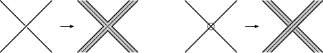
Figure 3. The bands for a classical and virtual crossing.

Given a virtual knot or link diagram $K$, there is a canonical surface $\Sigma_{K}$ called the Carter surface which contains a knot or link representing $K$. We review the construction of $\Sigma_{K}$, following the treatment of N. Kamada and S. Kamada in [17]. (The reader may also want to consult Carter’s paper [6].) The surface $\Sigma_{K}$ is constructed by attaching two intersecting bands at every classical crossing and two non-intersecting bands at every virtual crossing, see Figure 3. Along the remaining arcs of $K$ attach non-intersecting and non-twisted bands, and the result is an oriented 2-manifold with boundary. By filling in each boundary component with a 2-disk, one obtains a closed oriented surface $\Sigma_{K}$ containing a representative of $K$.

Two virtual knots or links are said to be welded equivalent if one can be obtained from the other by generalized Reidemeister moves plus the forbidden overpass ($f1$) in Figure 1. In terms of Gauss diagrams, this move corresponds to exchanging two adjacent arrow feet, see Figure 4.

Figure 4. The forbidden overpass $(f1)$ for Gauss diagrams.

2. Group-valued invariants of virtual knots

In this section, we introduce a family of group-valued invariants of virtual knots. We begin with the knot group $G_{K}$.

Suppose $K$ is an oriented virtual knot with $n$ classical crossings, and choose a basepoint on K. Starting at the base point, we label the arcs $a_{1},a_{2},\ldots,a_{n}$ so that at each undercrossing, $a_{i}$ is the incoming arc and $a_{i+1}$ is the outgoing arc. We use a consistent labeling of the crossings so that the $i$-th crossing is as shown in Figure 5. For $i=1,\ldots,,n$ let $\varepsilon_{i}=\pm 1$ be according to the sign of the $i$-th crossing. Then the knot group of $K$ is the finitely presented group given by

$$G_{K}=\langle a_{1},\ldots,a_{n}\mid a_{i+1}=a_{j}^{\varepsilon_{i}}a_{i}a_{j}^{-\varepsilon_{i}},i=1,\ldots,n\rangle.$$

Note that virtual crossings are ignored in this construction.

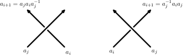
Figure 5. The relations in $G_{K}$ from the $i$-th crossing of $K$.

The knot group $G_{K}$ is invariant under all the moves in Figure 1 including the forbidden overpass ($f1$), thus it is an invariant of the underlying welded equivalence class of $K$. In case $K$ is classical, we have $G_{K}\cong\pi_{1}(S^{3}\smallsetminus N(K)),$ the fundamental group of the complement of $K$.

The virtual knot group $\operatorname{\it VG}_{K}$ was introduced in [3]; it has one generator for each short arc of $K$ and two commuting generators $s$ and $q$, and there are two relations for each real and virtual crossing as in Figure 6. Here the short arcs of $K$ are arcs that start at one real or virtual crossing and end at the next real or virtual crossing.

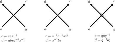
Figure 6. The crossing relations for the virtual knot group $\operatorname{\it VG}_{K}$.

The virtual knot group $\operatorname{\it VG}_{K}$ has as quotients various other knot groups that arise naturally in virtual knot theory. For instance, setting $q=s$, one obtains the welded knot group $\operatorname{\it WG}_{K}$, which is easily seen to be invariant under welded equivalence (see [3]). By setting $s=1$, one obtains the quandle group $\operatorname{\it QG}_{K}$, which was first introduced by Manturov in [23] and further studied by Bardakov and Bellingeri in [2].

By setting $q=1$ one obtains the extended group $\operatorname{\it EG}_{K}$, which was introduced by Silver and Williams in [34], where it is denoted by $\widetilde{\pi}_{K}$. The extended group is closely related to the Alexander group, a countably presented group invariant of virtual knots that Silver and Williams use to define the generalized Alexander polynomial $G_{K}(s,t)$, see [31].

The following diagram summarizes the relationship between $\operatorname{\it VG}_{K},\operatorname{\it QG}_{K},$ $\operatorname{\it WG}_{K},\operatorname{\it EG}_{K},$ and $G_{K}$.

A commutative diamond for the augmented knot groups.

Notice that the constructions of $G_{K}$ and $\operatorname{\it EG}_{K}$ make no reference to virtual crossings, and in fact for both knots the virtual crossing relations are trivial. Consequently, one can describe these groups entirely in terms of the Gauss diagram for $K$, which is advantageous in applying computer algorithms to perform algebraic computations. The constructions of $\operatorname{\it QG}_{K}$ and $\operatorname{\it VG}_{K}$ involve non-trivial virtual crossing relations, and so it is not immediately clear how to describe either of these groups in terms of Gauss diagrams. In the next section, we will introduce the reduced virtual knot group $\operatorname{\it\hbox{ \kern 0.09995pt\vbox{\hrule height=0.5pt\kern 1.07639pt\hbox{\kern-1.99997pt$G$\kern-0.50003pt}}\kern-0.29999pt}}_{K}$, and this group has the advantage of being computable from the Gauss diagram and we will see that it determines the virtual knot group $\operatorname{\it VG}_{K}$ and the quandle group $\operatorname{\it QG}_{K}$.

3. The reduced virtual knot group

In this section, we introduce the reduced knot group $\operatorname{\it\hbox{ \kern 0.09995pt\vbox{\hrule height=0.5pt\kern 1.07639pt\hbox{\kern-1.99997pt$G$\kern-0.50003pt}}\kern-0.29999pt}}_{K}$ and show that the virtual knot group $\operatorname{\it VG}_{K}$ can be reconstituted from $\operatorname{\it\hbox{ \kern 0.09995pt\vbox{\hrule height=0.5pt\kern 1.07639pt\hbox{\kern-1.99997pt$G$\kern-0.50003pt}}\kern-0.29999pt}}_{K}$. We then prove that $\operatorname{\it\hbox{ \kern 0.09995pt\vbox{\hrule height=0.5pt\kern 1.07639pt\hbox{\kern-1.99997pt$G$\kern-0.50003pt}}\kern-0.29999pt}}_{K}$ is isomorphic to both the quandle group $\operatorname{\it QG}_{K}$ and the extended knot $\operatorname{\it EG}_{K}$.

Figure 7. The crossing relations for the reduced virtual knot group $\operatorname{\it\hbox{ \kern 0.09995pt\vbox{\hrule height=0.5pt\kern 1.07639pt\hbox{\kern-1.99997pt$G$\kern-0.50003pt}}\kern-0.29999pt}}_{K}$.

Let $K$ be a virtual knot. The reduced virtual knot group $\operatorname{\it\hbox{ \kern 0.09995pt\vbox{\hrule height=0.5pt\kern 1.07639pt\hbox{\kern-1.99997pt$G$\kern-0.50003pt}}\kern-0.29999pt}}_{K}$ has a Wirtinger presentation with generators given by the arcs of $K$ as labeled in Figure 7 along with the augmentation generator $v$. There are two relations for each classical crossing, as in Figure 7, and virtual crossings are ignored.

The first result in this section explains the relationship between the reduced virtual knot group $\operatorname{\it\hbox{ \kern 0.09995pt\vbox{\hrule height=0.5pt\kern 1.07639pt\hbox{\kern-1.99997pt$G$\kern-0.50003pt}}\kern-0.29999pt}}_{K}$ and $\operatorname{\it VG}_{K}$. The proof will use the notion of an Alexander numbering, which we will define next.

Let $\Gamma$ be a 4-valent oriented graph and let $S$ be the set of edges of $\Gamma$. We say that $\Gamma$ has an Alexander numbering if there exists a function $\lambda\colon S\to{\mathbb{Z}}$ satisfying the relations in Figure 8 at each vertex. A standard argument using winding numbers shows that any (classical) knot diagram admits an Alexander numbering. This was first observed by Alexander in [1], and the argument uses the fact that an Alexander numbering of a knot diagram $\Gamma$ is equivalent to a numbering of the regions of ${\mathbb{R}}^{2}\smallsetminus\Gamma$ by the convention where a region $R$ has the number $\lambda_{a}$ for any edge $a$ with $R$ to its right, see Fig. 2 of [1]

Figure 8. The Alexander numbering of $\Gamma$.

Theorem 3.1.

If $K$ is a virtual knot or link, then $\operatorname{\it VG}_{K}=\operatorname{\it\hbox{ \kern 0.09995pt\vbox{\hrule height=0.5pt\kern 1.07639pt\hbox{\kern-1.99997pt$G$\kern-0.50003pt}}\kern-0.29999pt}}_{K}*_{\mathbb{Z}}\;{\mathbb{Z}}^{2}$.

Proof.

To prove this result, we will make a change of variables that depends on an Alexander numbering of the underlying $4$-valent planar graph associated to $K$. Flatten $K$ by replacing classical and virtual crossings with $4$-valent vertices. Denote the resulting planar graph as $\Gamma$, and note that since $\Gamma$ is planar, it admits an Alexander numbering. (In Section 5, we will introduce Alexander numberings for virtual knots, and we will see that not all virtual knots are Alexander numberable.)

We use the Alexander numbering to make a change of variables. Starting with the generators and crossing relations of $\operatorname{\it VG}_{K}$ from Figure 6, make the substitution

(1) $$\left\{\begin{array}[]{lll}a^{\prime}&=&q^{\lambda_{a}}\,a\,q^{-\lambda_{a}}\\ b^{\prime}&=&q^{\lambda_{b}}\,b\,q^{-\lambda_{b}}\\ c^{\prime}&=&q^{\lambda_{c}}\,c\,q^{-\lambda_{c}}\\ d^{\prime}&=&q^{\lambda_{d}}\,d\,q^{-\lambda_{d}}.\end{array}\right.$$

In terms of the new generators $a^{\prime},b^{\prime},c^{\prime},d^{\prime}$, it follows that $\operatorname{\it VG}_{K}$ has crossing relations as in Figure 9.

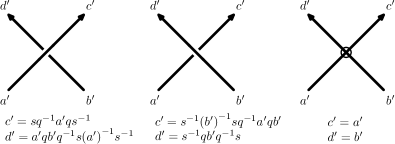
Figure 9. The transformed crossing relations for $\operatorname{\it VG}_{K}$.

We make a further change of variables in $\operatorname{\it VG}_{K}$ by setting $a^{\prime\prime}=a^{\prime}s,b^{\prime\prime}=b^{\prime}s,c^{\prime\prime}=c^{\prime}s,$ and $d^{\prime\prime}=d^{\prime}s$. Upon substituting $v$ for $sq^{-1}$ and noting that $s$ and $q$ commute in $\operatorname{\it VG}_{K}$, in terms of the new generators $a^{\prime\prime},b^{\prime\prime},c^{\prime\prime},d^{\prime\prime}$, it is not difficult to check that the crossing relations for $\operatorname{\it VG}_{K}$ are identical to the relations for $\operatorname{\it\hbox{ \kern 0.09995pt\vbox{\hrule height=0.5pt\kern 1.07639pt\hbox{\kern-1.99997pt$G$\kern-0.50003pt}}\kern-0.29999pt}}_{K}$ in Figure 7. ∎

Remark 3.2.

A similar change of variables was used by Silver and Williams in their proof of [34, Proposition 4.2].

In the next result, we use the reduced virtual knot group $\operatorname{\it\hbox{ \kern 0.09995pt\vbox{\hrule height=0.5pt\kern 1.07639pt\hbox{\kern-1.99997pt$G$\kern-0.50003pt}}\kern-0.29999pt}}_{K}$ to construct isomorphisms between the quandle group $\operatorname{\it QG}_{K}$ and the extended group $\operatorname{\it EG}_{K}$.

Theorem 3.3.

If $K$ is a virtual knot or link, then the extended group $\operatorname{\it EG}_{K}$ and the quandle group $\operatorname{\it QG}_{K}$ are both isomorphic to the reduced virtual knot group $\operatorname{\it\hbox{ \kern 0.09995pt\vbox{\hrule height=0.5pt\kern 1.07639pt\hbox{\kern-1.99997pt$G$\kern-0.50003pt}}\kern-0.29999pt}}_{K}$.

Proof.

We first argue that $\operatorname{\it\hbox{ \kern 0.09995pt\vbox{\hrule height=0.5pt\kern 1.07639pt\hbox{\kern-1.99997pt$G$\kern-0.50003pt}}\kern-0.29999pt}}_{K}$ is isomorphic to $\operatorname{\it EG}_{K}$. To see this, we make the change of variables $a^{\prime}=av^{-1},b^{\prime}=bv^{-1},c^{\prime}=cv^{-1},$ and $d^{\prime}=dv^{-1}$ in $\operatorname{\it\hbox{ \kern 0.09995pt\vbox{\hrule height=0.5pt\kern 1.07639pt\hbox{\kern-1.99997pt$G$\kern-0.50003pt}}\kern-0.29999pt}}_{K}$. Upon setting $v=s$, the crossing relations in the new variables $a^{\prime},b^{\prime},c^{\prime},d^{\prime}$ are identical with the crossing relations for $\operatorname{\it EG}_{K}$.

To show that $\operatorname{\it QG}_{K}$ is isomorphic to $\operatorname{\it\hbox{ \kern 0.09995pt\vbox{\hrule height=0.5pt\kern 1.07639pt\hbox{\kern-1.99997pt$G$\kern-0.50003pt}}\kern-0.29999pt}}_{K}$, we flatten $K$ by replacing classical and virtual crossings with $4$-valent vertices and denote the resulting planar graph as $\Gamma$. Since $\Gamma$ is planar, it admits an Alexander numbering which we use to perform a change of variables to the meridional generators of $\operatorname{\it QG}_{K}$ as in Equation (1).

In terms of the new generators $a^{\prime},b^{\prime},c^{\prime},d^{\prime}$, the crossing relations for $\operatorname{\it QG}_{K}$ are easily seen to be identical to the relations for $\operatorname{\it\hbox{ \kern 0.09995pt\vbox{\hrule height=0.5pt\kern 1.07639pt\hbox{\kern-1.99997pt$G$\kern-0.50003pt}}\kern-0.29999pt}}_{K}$ in Figure 7. This completes the proof. ∎

The following diagram summarizes the results of Theorem 3.1 and 3.3. The injective map $\operatorname{\it\hbox{ \kern 0.09995pt\vbox{\hrule height=0.5pt\kern 1.07639pt\hbox{\kern-1.99997pt$G$\kern-0.50003pt}}\kern-0.29999pt}}_{K}\hookrightarrow\operatorname{\it VG}_{K}$ is induced by the map $\operatorname{\it\hbox{ \kern 0.09995pt\vbox{\hrule height=0.5pt\kern 1.07639pt\hbox{\kern-1.99997pt$G$\kern-0.50003pt}}\kern-0.29999pt}}_{K}\,*_{\mathbb{Z}}\;{\mathbb{Z}}\hookrightarrow\operatorname{\it\hbox{ \kern 0.09995pt\vbox{\hrule height=0.5pt\kern 1.07639pt\hbox{\kern-1.99997pt$G$\kern-0.50003pt}}\kern-0.29999pt}}_{K}\,*_{\mathbb{Z}}\;{\mathbb{Z}}^{2}$ sending $v\mapsto sq^{-1}$, noting the isomorphisms $\operatorname{\it\hbox{ \kern 0.09995pt\vbox{\hrule height=0.5pt\kern 1.07639pt\hbox{\kern-1.99997pt$G$\kern-0.50003pt}}\kern-0.29999pt}}_{K}\,\cong\operatorname{\it\hbox{ \kern 0.09995pt\vbox{\hrule height=0.5pt\kern 1.07639pt\hbox{\kern-1.99997pt$G$\kern-0.50003pt}}\kern-0.29999pt}}_{K}\,*_{\mathbb{Z}}\;{\mathbb{Z}}$ and $\operatorname{\it VG}_{K}\cong\operatorname{\it\hbox{ \kern 0.09995pt\vbox{\hrule height=0.5pt\kern 1.07639pt\hbox{\kern-1.99997pt$G$\kern-0.50003pt}}\kern-0.29999pt}}_{K}\,*_{\mathbb{Z}}\;{\mathbb{Z}}^{2}.$

A commutative diamond for the augmented knot groups.

Because the crossing relations for the reduced group $\operatorname{\it\hbox{ \kern 0.09995pt\vbox{\hrule height=0.5pt\kern 1.07639pt\hbox{\kern-1.99997pt$G$\kern-0.50003pt}}\kern-0.29999pt}}_{K}$ do not involve the virtual crossings, it follows that $\operatorname{\it\hbox{ \kern 0.09995pt\vbox{\hrule height=0.5pt\kern 1.07639pt\hbox{\kern-1.99997pt$G$\kern-0.50003pt}}\kern-0.29999pt}}_{K}$ can be determined directly from a Gauss diagram for $K$. This has the following consequence.

Corollary 3.4.

For any virtual knot or link $K$, the virtual knot group $\operatorname{\it VG}_{K}$ and the quandle group $\operatorname{\it QG}_{K}$ can be calculated from a Gauss diagram of $K$.

As we have already noted, the group obtained from $\operatorname{\it VG}_{K}$ upon setting $s=q$ is invariant under welded equivalence, cf. [3]. This group is denoted $\operatorname{\it WG}_{K}$ and is called the welded knot group. The next result shows that the welded knot group $\operatorname{\it WG}_{K}$ splits as a free product of the knot group $G_{K}$ and ${\mathbb{Z}}.$

Proposition 3.5.

If $K$ is a welded knot or link, then $\operatorname{\it WG}_{K}=G_{K}*{\mathbb{Z}}$.

Proof.

Let $K$ be virtual knot, then $\operatorname{\it WG}_{K}$ is the group generated by the short arcs of $K$ and one auxiliary variable $s$ with relations at each real or virtual crossing as in Figure 6 (setting $q=s$).

We flatten $K$ by replacing classical and virtual crossings with $4$-valent vertices. Denote the resulting graph as $\Gamma$. Since $\Gamma$ is planar, it admits an Alexander numbering, which we use to make the following change of variables:

(2) $$\left\{\begin{array}[]{lll}a^{\prime}&=&s^{\lambda_{a}}\,a\,s^{-\lambda_{a}}\\ b^{\prime}&=&s^{\lambda_{b}}\,b\,s^{-\lambda_{b}}\\ c^{\prime}&=&s^{\lambda_{c}}\,c\,s^{-\lambda_{c}}\\ d^{\prime}&=&s^{\lambda_{d}}\,d\,s^{-\lambda_{d}}.\end{array}\right.$$

In terms of the new generators $a^{\prime},b^{\prime},c^{\prime},d^{\prime},$ the crossing relations in $\operatorname{\it WG}_{K}$ transform into those in Figure 10.

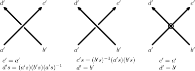
Figure 10. The crossing relations for the welded knot group $\operatorname{\it WG}_{K}$

We make a further change of variables by setting $a^{\prime\prime}=a^{\prime}s,b^{\prime\prime}=b^{\prime}s,c^{\prime\prime}=c^{\prime}s,d^{\prime\prime}=d^{\prime}s$, and in the new generators, one can easily see that the crossing relations are identical to those of $G_{K}$. ∎

We conclude this section by outlining an alternate approach to proving Theorem 3.1 and Proposition 3.5 that involves the virtual braid group.

The virtual braid group on $k$ strands, $\operatorname{\it VB}_{k}$, is defined by generators $\sigma_{1},\ldots,\sigma_{k-1}$ and $\tau_{1},\ldots,\tau_{k-1}$ subject to the relations:

$$\begin{array}[]{rcl}\sigma_{i}\sigma_{j}&=&\sigma_{j}\sigma_{i}\hskip 42.67912pt\text{ if $|i-j|>1$,}\\ \sigma_{i}\sigma_{i+1}\sigma_{i}&=&\sigma_{i+1}\sigma_{i}\sigma_{i+1},\\ \\ \tau_{i}\tau_{j}&=&\tau_{j}\tau_{i}\hskip 42.67912pt\text{ if $|i-j|>1$,}\\ \tau_{i}\tau_{i+1}\tau_{i}&=&\tau_{i+1}\tau_{i}\tau_{i+1},\\ \tau_{i}^{2}&=&1,\\ \\ \sigma_{i}\tau_{j}&=&\tau_{j}\sigma_{i}\hskip 42.67912pt\text{ if $|i-j|>1$,}\\ \tau_{i}\sigma_{i+1}\tau_{i}&=&\tau_{i+1}\sigma_{i}\tau_{i+1}.\end{array}$$

The generator $\sigma_{i}$ is represented by a braid in which the $i$-th strand crosses over the $(i+1)$-st strand and the generator $\tau_{i}$ is represented by a braid in which the $i$-th strand virtually crosses the $(i+1)$-st strand.

We recall the fundamental representation of $\operatorname{\it VB}_{k}$ from [3, §4]. For each $i=1,\ldots,k-1$, define automorphisms $\Phi(\sigma_{i})$ and $\Phi(\tau_{i})$ of the free group $F_{k+2}=\langle x_{1},\ldots,x_{k},s,q\rangle$ fixing $s$ and $q$ as follows. For $j=1,\ldots,k$,

(3) $$\begin{split}(x_{j})\Phi(\sigma_{i})=&\begin{cases}sx_{i+1}s^{-1}&\text{if $j=i$,}\\ x_{i+1}x_{i}(sx_{i+1}^{-1}s^{-1})&\text{if $j=i+1$,}\\ x_{j}&\text{otherwise},\end{cases}\\ (x_{j})\Phi(\tau_{i})=&\begin{cases}qx_{i+1}q^{-1}&\text{if $j=i$,}\\ q^{-1}x_{i}q&\text{if $j=i+1$,}\\ x_{j}&\text{otherwise}.\end{cases}\end{split}$$

Consider the following free basis for $F_{k+2}$:

$${\bar{x}_{i}}=\big{(}q^{i-1}x_{i}\,q^{-i+1}\big{)}q=q^{i-1}x_{i}\,q^{-i+2}\text{ for }1\leq i\leq k,\,v=sq^{-1},\text{ and }s.$$

Note we can use $q$ in place of $s$ for the last element of the basis.

A straightforward calculation gives the action of $\Phi(\sigma_{i})$ and $\Phi(\tau_{i})$ on the new basis, yielding:

(4) $$\begin{split}({\bar{x}}_{j})\Phi(\sigma_{i})=&\begin{cases}v{\bar{x}}_{i+1}v^{-1}&\text{if $j=i$,}\\ {\bar{x}}_{i+1}{\bar{x}}_{i}(v{\bar{x}}_{i+1}^{-1}v^{-1})&\text{if $j=i+1$,}\\ {\bar{x}}_{j}&\text{otherwise},\end{cases}\\ ({\bar{x}}_{j})\Phi(\tau_{i})=&\begin{cases}{\bar{x}}_{i+1}&\text{if $j=i$,}\\ {\bar{x}}_{i}&\text{if $j=i+1$,}\\ {\bar{x}}_{j}&\text{otherwise}.\end{cases}\end{split}$$

and $v$ and $s$ (and $q$) are fixed by $\Phi(\sigma_{i})$ and $\Phi(\tau_{i})$.

This calculation can be viewed as the non-abelian version of [3, Theorem 4.5], that is, taking place in $\operatorname{Aut}(F_{k+2})$.

If $K=\widehat{\beta}$ is the closure of $\beta\in\operatorname{\it VB}_{k}$, then the virtual knot group $\operatorname{\it VG}_{K}$ admits the presentation

(5) $$\langle{\bar{x}}_{1},\ldots,{\bar{x}}_{k},v,s\mid{\bar{x}}_{1}={\bar{x}}_{1}^{\beta},\ldots,{\bar{x}}_{k}={\bar{x}}_{k}^{\beta},[v,s]=1\rangle.$$

Observe that $s$ does not appear in ${\bar{x}}_{i}^{\beta}$ for $i=1,\ldots,k,$ and setting $s=1$ in (5) one obtains a presentation for the reduced virtual knot group $\operatorname{\it\hbox{ \kern 0.09995pt\vbox{\hrule height=0.5pt\kern 1.07639pt\hbox{\kern-1.99997pt$G$\kern-0.50003pt}}\kern-0.29999pt}}_{K},$ whereas setting $v=1$ in (5) one obtains a presentation for the welded knot group $\operatorname{\it WG}_{K}.$ It now follows easily from (5) that $\operatorname{\it WG}_{K}=G_{K}*{\mathbb{Z}}$ ($v$ goes to $1$) and $\operatorname{\it VG}_{K}=\operatorname{\it\hbox{ \kern 0.09995pt\vbox{\hrule height=0.5pt\kern 1.07639pt\hbox{\kern-1.99997pt$G$\kern-0.50003pt}}\kern-0.29999pt}}\,*_{\mathbb{Z}}\;{\mathbb{Z}}^{2}$.

4. Virtual Alexander invariants

In this section, we introduce the Alexander invariants of the knot group $G_{K}$ and the reduced virtual knot group $\operatorname{\it\hbox{ \kern 0.09995pt\vbox{\hrule height=0.5pt\kern 1.07639pt\hbox{\kern-1.99997pt$G$\kern-0.50003pt}}\kern-0.29999pt}}_{K}$.

We begin by recalling the construction of the Alexander invariants for the knot group $G_{K}=\langle a_{1},\ldots,a_{n}\mid r_{1},\ldots,r_{n}\rangle.$ Let $G_{K}^{\prime}=[G_{K},G_{K}]$ and $G_{K}^{\prime\prime}=[G_{K}^{\prime},G_{K}^{\prime}]$ be the first and second commutator subgroups, then the Alexander module is defined to be the quotient $G_{K}^{\prime}/G_{K}^{\prime\prime}.$ It is finitely generated as a module over the ring ${\mathbb{Z}}[t^{\pm 1}]$, and it can be completely described in terms of a presentation matrix $A$, which is the $n\times n$ matrix obtained by Fox differentiating the relations $r_{i}$ of $G_{K}$ with respect to the generators $a_{j}$. While the matrix $A$ will depend on the choice of presentation for $G_{K}$, the associated sequence of elementary ideals

(6) $$(0)=\mathcal{E}_{0}\subset\mathcal{E}_{1}\subset\cdots\subset\mathcal{E}_{n}={\mathbb{Z}}[t^{\pm 1}]$$

does not. Here, the $k$-th elementary ideal $\mathcal{E}_{k}$ is defined as the ideal of ${\mathbb{Z}}[t^{\pm 1}]$ generated by all $(n-k)\times(n-k)$ minors of $A$. The Alexander invariants of $K$ are then defined in terms of the ideals (6), and since $G_{K}$ is an invariant of the welded type, these ideals are welded invariants of $K$.

For purely algebraic reasons, the zeroth elementary ideal $\mathcal{E}_{0}$ is always trivial, and the reason is that the fundamental identity of Fox derivatives implies that one column of $A$ can be written as a linear combination of the other columns. This is true for both classical and virtual knots, and it is an algebraic defect of the knot group $G_{K}$.

Replacing $G_{K}$ by the reduced virtual knot group $\operatorname{\it\hbox{ \kern 0.09995pt\vbox{\hrule height=0.5pt\kern 1.07639pt\hbox{\kern-1.99997pt$G$\kern-0.50003pt}}\kern-0.29999pt}}_{K}$, we will see that one obtains an interesting invariant from the zeroth elementary ideal of the associated Alexander module. In [3], we introduce virtual Alexander invariants of $K$, which are defined in terms of the Alexander ideals of the virtual knot group $\operatorname{\it VG}_{K}$. Since $\operatorname{\it VG}_{K}$ abelianizes to ${\mathbb{Z}}^{3}$, its Alexander module is a module over ${\mathbb{Z}}[s^{\pm 1},t^{\pm 1},q^{\pm 1}]$. The zeroth order elementary ideal is typically non-trivial, and we define $H_{K}(s,t,q)$ to be the generator of the smallest principal ideal containing it. Thus $H_{K}(s,t,q)$ is an invariant of virtual knots, and in [3], we show that $H_{K}(s,t,q)$ admits a normalization, satisfies a skein formula, and carries information about the virtual crossing number of $K$. In [3], we proved a formula relating the virtual Alexander polynomial $H_{K}(s,t,q)$ to the generalized Alexander polynomial $G_{K}(s,t)$ defined by Sawollek [30], and in equivalent forms by Kauffman–Radford [19], Manturov [23], and Silver–Williams [31, 32]. Specifically, Corollary 4.8 of [3] shows that

$$H_{K}(s,t,q)=G_{K}(sq^{-1},tq).$$

Theorem 3.1 implies that the Alexander module of $\operatorname{\it\hbox{ \kern 0.09995pt\vbox{\hrule height=0.5pt\kern 1.07639pt\hbox{\kern-1.99997pt$G$\kern-0.50003pt}}\kern-0.29999pt}}_{K}$ contains the same information as the Alexander module of $\operatorname{\it VG}_{K},$ and Theorem 3.3 shows the same is true for the Alexander modules of the quandle group $\operatorname{\it QG}_{K}$ and the extended group $\operatorname{\it EG}_{K}$. We shall therefore focus our efforts on understanding the Alexander invariants associated to $\operatorname{\it\hbox{ \kern 0.09995pt\vbox{\hrule height=0.5pt\kern 1.07639pt\hbox{\kern-1.99997pt$G$\kern-0.50003pt}}\kern-0.29999pt}}_{K}\cong\operatorname{\it QG}_{K}\cong\operatorname{\it EG}_{K}$.

Let $\operatorname{\it\hbox{ \kern 0.09995pt\vbox{\hrule height=0.5pt\kern 1.07639pt\hbox{\kern-1.99997pt$G$\kern-0.50003pt}}\kern-0.29999pt}}_{K}=\langle a_{1},\ldots,a_{n},v\mid r_{1},\ldots,r_{n}\rangle$ be a presentation of the reduced virtual knot group. Its Alexander module is defined to be the quotient ${\operatorname{\it\hbox{ \kern 0.09995pt\vbox{\hrule height=0.5pt\kern 1.07639pt\hbox{\kern-1.99997pt$G$\kern-0.50003pt}}\kern-0.29999pt}}^{\,\prime}_{K}}/\operatorname{\it\hbox{ \kern 0.09995pt\vbox{\hrule height=0.5pt\kern 1.07639pt\hbox{\kern-1.99997pt$G$\kern-0.50003pt}}\kern-0.29999pt}}_{K}^{\,\prime\prime},$ where $\operatorname{\it\hbox{ \kern 0.09995pt\vbox{\hrule height=0.5pt\kern 1.07639pt\hbox{\kern-1.99997pt$G$\kern-0.50003pt}}\kern-0.29999pt}}_{K}^{\,\prime}$ and $\operatorname{\it\hbox{ \kern 0.09995pt\vbox{\hrule height=0.5pt\kern 1.07639pt\hbox{\kern-1.99997pt$G$\kern-0.50003pt}}\kern-0.29999pt}}_{K}^{\,\prime\prime}$ denote the first and second commutator subgroups of $\operatorname{\it\hbox{ \kern 0.09995pt\vbox{\hrule height=0.5pt\kern 1.07639pt\hbox{\kern-1.99997pt$G$\kern-0.50003pt}}\kern-0.29999pt}}_{K}$. It is finitely generated as a module over ${\mathbb{Z}}[t^{\pm t},v^{\pm 1}]$, and one obtains a presentation matrix for it by Fox differentiating the relations of $\operatorname{\it\hbox{ \kern 0.09995pt\vbox{\hrule height=0.5pt\kern 1.07639pt\hbox{\kern-1.99997pt$G$\kern-0.50003pt}}\kern-0.29999pt}}_{K}$ with respect to the generators. Specifically, the $n\times(n+1)$ matrix

$$M=\begin{bmatrix}A&\left(\frac{\partial r}{\partial v}\right)\end{bmatrix}$$

is a presentation matrix for this module. Here the $(i,j)$-th entry of $A$ is given by $\left.\frac{\partial r_{i}}{\partial a_{j}}\right|_{a_{1},\ldots,a_{n}=t}$ and $\left(\frac{\partial r}{\partial v}\right)$ is a column vector with $i$-th entry given by $\left.\frac{\partial r_{i}}{\partial v}\right|_{a_{1},\ldots,a_{n}=t}$. Let

(7) $$(0)\subset\bar{\mathcal{E}}_{0}\subset\bar{\mathcal{E}}_{1}\subset\cdots\subset\bar{\mathcal{E}}_{n}={\mathbb{Z}}[t^{\pm 1}]$$

denote the sequence of elementary ideals, where $\bar{\mathcal{E}}_{k}$ is the ideal of ${\mathbb{Z}}[t^{\pm 1},v^{\pm 1}]$ generated by the $(n-k)\times(n-k)$ minors of $M$. The $k$-th Alexander polynomial $\bar{\Delta}^{\ell}_{K}(t,v)$ is defined to be the generator for the smallest principal ideal containing $\bar{\mathcal{E}}_{k}$; alternatively it is given by the $\gcd$ of the $(n-k)\times(n-k)$ minors of $M$.

We use $\hbox{ \kern 0.09995pt\vbox{\hrule height=0.5pt\kern 1.07639pt\hbox{\kern-1.99997pt$H$\kern-0.50003pt}}\kern-0.29999pt}_{K}(t,v)=\bar{\Delta}^{0}_{K}(t,v)$ to denote the zeroth Alexander polynomial associated to $\operatorname{\it\hbox{ \kern 0.09995pt\vbox{\hrule height=0.5pt\kern 1.07639pt\hbox{\kern-1.99997pt$G$\kern-0.50003pt}}\kern-0.29999pt}}_{K}$. Note that $\hbox{ \kern 0.09995pt\vbox{\hrule height=0.5pt\kern 1.07639pt\hbox{\kern-1.99997pt$H$\kern-0.50003pt}}\kern-0.29999pt}_{K}(t,v)$ is well-defined up to multiplication by units in ${\mathbb{Z}}[t^{\pm 1},v^{\pm 1}]$ and is closely related to the virtual Alexander polynomial $H_{K}(s,t,q)$ and the generalized Alexander polynomial $G_{K}(s,t)$. In particular, one can define a normalization of $\hbox{ \kern 0.09995pt\vbox{\hrule height=0.5pt\kern 1.07639pt\hbox{\kern-1.99997pt$H$\kern-0.50003pt}}\kern-0.29999pt}_{K}(t,v)$ using braids by following the approach in Section 5 of [3], and one can also derive lower bounds on $v(K)$, the virtual crossing number of $K$, from $\hbox{ \kern 0.09995pt\vbox{\hrule height=0.5pt\kern 1.07639pt\hbox{\kern-1.99997pt$H$\kern-0.50003pt}}\kern-0.29999pt}_{K}(t,v)$ and its normalization.

Theorem 4.1.

The generalized Alexander polynomial $G_{K}(s,t)$ is related to the reduced Alexander polynomial $\hbox{ \kern 0.09995pt\vbox{\hrule height=0.5pt\kern 1.07639pt\hbox{\kern-1.99997pt$H$\kern-0.50003pt}}\kern-0.29999pt}_{K}(t,v)$ by the formula

$$G_{K}(s,t)=\hbox{ \kern 0.09995pt\vbox{\hrule height=0.5pt\kern 1.07639pt\hbox{\kern-1.99997pt$H$\kern-0.50003pt}}\kern-0.29999pt}_{K}(st,s).$$

Proof.

Choose a presentation for the reduced virtual knot group $\operatorname{\it\hbox{ \kern 0.09995pt\vbox{\hrule height=0.5pt\kern 1.07639pt\hbox{\kern-1.99997pt$G$\kern-0.50003pt}}\kern-0.29999pt}}_{K}$ with relations as in Figure 7. Given a word $w$ in $a_{1},\ldots,a_{n},v$ and an automorphism $f\in\operatorname{Aut}(F_{n+1})$, we write $w^{f}$ for the word obtained by applying $f$ to $w$. Notice that this extends to give an automorphism of the group ring ${\mathbb{Z}}[F_{n+1}].$ If $r_{i}$ is a relator of $\operatorname{\it\hbox{ \kern 0.09995pt\vbox{\hrule height=0.5pt\kern 1.07639pt\hbox{\kern-1.99997pt$G$\kern-0.50003pt}}\kern-0.29999pt}}_{K}$, then we see that $\tilde{r}_{i}={r_{i}}^{f}$ is a relator of $\operatorname{\it EG}_{K}$ where $f$ is the automorphism that sends meridional generators $a_{j}\to a_{j}v$ and fixes the augmented generator $v$. Then by the chain rule for Fox derivatives, see Equation $2.6$ in [12], we have that

$$\frac{\partial\tilde{r}_{i}}{\partial a_{j}}=\frac{\partial(r_{i})^{f}}{\partial a_{j}}=\left(\frac{\partial{r_{i}}}{\partial a_{k}}\right)^{f}\frac{\partial a_{k}^{f}}{\partial a_{j}}.$$

After abelianizing, and multiplying by an appropriate unit, it follows that

$$\left(\frac{\partial\tilde{r}_{i}}{\partial a_{j}}\right)(v,t)=\left(\frac{\partial{r_{i}}}{\partial a_{j}}\right)(tv,v).$$

∎

In [3], we define twisted virtual Alexander invariants $H^{\varrho}_{K}(s,t,q)$ associated to representations $\varrho\colon\operatorname{\it VG}_{K}\to GL_{n}(R)$. The twisted virtual Alexander polynomials admit a natural normalization, and one can derive bounds on $v(K)$, the virtual crossing number of $K$ from $H^{\varrho}(s,t,q)$ and its normalization.

Using the reduced knot group $\operatorname{\it\hbox{ \kern 0.09995pt\vbox{\hrule height=0.5pt\kern 1.07639pt\hbox{\kern-1.99997pt$G$\kern-0.50003pt}}\kern-0.29999pt}}_{K}$ in place of $\operatorname{\it VG}_{K}$, one can similarly define twisted Alexander invariants $\hbox{ \kern 0.09995pt\vbox{\hrule height=0.5pt\kern 1.07639pt\hbox{\kern-1.99997pt$H$\kern-0.50003pt}}\kern-0.29999pt}^{\varrho}_{K}(t,v)$ associated to representations $\varrho\colon\operatorname{\it\hbox{ \kern 0.09995pt\vbox{\hrule height=0.5pt\kern 1.07639pt\hbox{\kern-1.99997pt$G$\kern-0.50003pt}}\kern-0.29999pt}}_{K}\to GL_{n}(R)$ by following the approach in [3, §7]. In particular, the twisted Alexander polynomial $\hbox{ \kern 0.09995pt\vbox{\hrule height=0.5pt\kern 1.07639pt\hbox{\kern-1.99997pt$H$\kern-0.50003pt}}\kern-0.29999pt}^{\varrho}_{K}(t,v)$ admits a normalization and carries information about the virtual crossing number $v(K)$ just as before, but it is easier to work with since $\operatorname{\it\hbox{ \kern 0.09995pt\vbox{\hrule height=0.5pt\kern 1.07639pt\hbox{\kern-1.99997pt$G$\kern-0.50003pt}}\kern-0.29999pt}}_{K}$ admits a presentation with fewer generators and relations than $\operatorname{\it VG}_{K}$.

5. Almost classical knots

In [34, Definition 4.3], Silver and Williams coined the term “almost classical knot” for any virtual knot $K$ represented by a diagram with an Alexander numbering, and in [8, Definition 2.4] they use mod 2 almost classical knot to refer to any virtual knot represented by a diagram with a mod $2$ Alexander numbering. The next definition provides a natural extension of these ideas by introducing the notion of a mod $p$ almost classical knot.

Definition 5.1.

1. Given an integer $p\geq 0$, we say that a virtual knot diagram is mod $p$ Alexander numberable if there exists an integer-valued function $\lambda$ on the set of short arcs satisfying the relations in Figure 11. In case $p=0,$ we say the diagram is Alexander numberable.

2. Given a virtual knot or link $K$, we say $K$ is mod $p$ almost classical if it admits a virtual knot diagram that is mod $p$ Alexander numberable. In case $p=0,$ we say that $K$ is almost classical.

Note that if a knot is almost classical, then it is mod $p$ almost classical for all $p$. Note also that when $p=1$ there is no condition on $K$, so we will assume $p\neq 1$ throughout.

By flattening classical and virtual crossings, as in Theorem 3.3, the resulting planar graph $\Gamma$ always has an Alexander numbering. The condition that a virtual knot diagram have an Alexander numbering is very restrictive. For instance, there are only four distinct non-trivial almost classical knots with up to four crossings, see Theorem $1.3$ of [28].

Definition 5.1 has natural interpretations for Gauss diagrams and for knots in surfaces as we now explain. For Gauss diagrams, this hinges on the fact that a Gauss diagram is mod $p$ Alexander numberable if and only if each chord $c_{i}$ has index $I(c_{i})=0$ mod $p$ (see Definition 1.1). The verification of this fact is not difficult and is left as an exercise.

For knots in surfaces, we claim that a knot $K$ in a thickened surface $\Sigma\times[0,1]$ is mod $p$ Alexander numberable if and only if it is homologically trivial as an element in $H_{1}(\Sigma;{\mathbb{Z}}/p),$ where ${\mathbb{Z}}/p$ denotes the cyclic group of order $p$. In case $p=2,$ the proof of this can be found in [8, §3]. (That argument also explains why, for a virtual knot diagram, the notion of a mod 2 Alexander numbering and checkerboard coloring coincide.) In general, recall from Section 1 that given a virtual knot diagram $K$, its Carter surface $\Sigma_{K}$ is constructed by first thickening the classical and virtual crossings of $K$ as in Figure 3 and then adding finitely many 2-disks $D_{1},\ldots,D_{n}$. Set $\Sigma=\Sigma_{K}$ and let $K$ be the associated knot in the thickened surface $\Sigma\times[0,1]$.

A mod $p$ Alexander numbering of $K$ induces a mod $p$ Alexander numbering of the 2-disks $D_{1},\ldots,D_{n}$ as follows. The Carter surface is built as a CW complex with 1-skeleton given by the thickening of $K$ and with 2-cells given by $D_{1},\ldots,D_{n}$. We number $D_{i}$ using the Alexander number of any edge $a$ of $K$ with $D_{i}$ to its right. Let $\lambda_{i}$ denote the associated number, and the conditions of Figure 8 guarantee that $\lambda_{i}$ is well-defined and independent of choice of edge. They further imply that for every edge of $K$, the Alexander number of the 2-disk to its right is exactly one more than the Alexander number of the 2-disk to its left. It follows that $\partial\left(\lambda_{1}D_{1}+\cdots+\lambda_{n}D_{n}\right)=K$ with coefficients in ${\mathbb{Z}}/p.$ Thus, if $K$ admits a mod $p$ Alexander numbering, then the associated knot in the surface is homologically trivial in $H_{1}(\Sigma;{\mathbb{Z}}/p).$ Conversely, if $K$ is a knot in $\Sigma\times[0,1]$ and is homologically trivial in $H_{1}(\Sigma;{\mathbb{Z}}/p)$, then that induces a mod $p$ Alexander numbering of the 2-disks $D_{1},\ldots,D_{n}$ of the Carter surface $\Sigma_{K}$, which in turn gives a mod $p$ Alexander numbering of $K$.

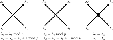
Figure 11. The mod $p$ Alexander numbering conditions.

The following theorem shows that $\operatorname{\it\hbox{ \kern 0.09995pt\vbox{\hrule height=0.5pt\kern 1.07639pt\hbox{\kern-1.99997pt$G$\kern-0.50003pt}}\kern-0.29999pt}}_{K}$ gives an obstruction for a virtual knot or link to be mod $p$ almost classical.

Theorem 5.2.

If $K$ is a mod $p$ almost classical knot or link, then it follows that $\operatorname{\it\hbox{ \kern 0.09995pt\vbox{\hrule height=0.5pt\kern 1.07639pt\hbox{\kern-1.99997pt$G$\kern-0.50003pt}}\kern-0.29999pt}}_{K}/\langle v^{p}\rangle\cong G_{K}*{\mathbb{Z}}/p$. If $K$ is almost classical, then $\operatorname{\it\hbox{ \kern 0.09995pt\vbox{\hrule height=0.5pt\kern 1.07639pt\hbox{\kern-1.99997pt$G$\kern-0.50003pt}}\kern-0.29999pt}}_{K}\cong G_{K}*{\mathbb{Z}}$.

Proof.

Suppose $K$ is mod $p$ almost classical knot and choose a diagram for it that admits a mod $p$ Alexander numbering. Consider the quotient group $\operatorname{\it\hbox{ \kern 0.09995pt\vbox{\hrule height=0.5pt\kern 1.07639pt\hbox{\kern-1.99997pt$G$\kern-0.50003pt}}\kern-0.29999pt}}_{K}/\langle v^{p}\rangle$ obtained by adding the relation $v^{p}=1$, and make the following change of variables to the generators of Figure 7 according to the mod $p$ Alexander numbering of Figure 11:

$$\begin{array}[]{lll}a^{\prime}&=&v^{\lambda_{a}}\,a\,v^{-\lambda_{a}}\\ b^{\prime}&=&v^{\lambda_{b}}\,b\,v^{-\lambda_{b}}\\ c^{\prime}&=&v^{\lambda_{c}}\,c\,v^{-\lambda_{c}}\\ d^{\prime}&=&v^{\lambda_{d}}\,d\,v^{-\lambda_{d}}.\end{array}$$

It is not difficult to check that, in the new generators $a^{\prime},b^{\prime},c^{\prime},d^{\prime},$ the crossing relations coincide with those for $G_{K}$. ∎

Example 5.3.

We will use Theorem 5.2 to see that the virtual knot $K=4.41$ depicted in Figure 12 is not mod 2 almost classical. Since this knot has $\hbox{ \kern 0.09995pt\vbox{\hrule height=0.5pt\kern 1.07639pt\hbox{\kern-1.99997pt$H$\kern-0.50003pt}}\kern-0.29999pt}_{K}(t,v)=0$, we are unable to conclude this from Corollary 5.4 below.

Since $K$ is welded trivial, its knot group $G_{K}\cong\langle a\rangle$ is trivial. Using sage, we determine that $K$ has reduced virtual knot group

$$\operatorname{\it\hbox{ \kern 0.09995pt\vbox{\hrule height=0.5pt\kern 1.07639pt\hbox{\kern-1.99997pt$G$\kern-0.50003pt}}\kern-0.29999pt}}_{K} = \langle a,v\mid va^{-1}v^{-3}a^{-1}v^{2}a^{-1}v^{-2}av^{3}a(v^{-1}a^{-1})^{2}\cdot$$

$$\hskip 42.67912ptv^{2}av^{-2}(av)^{2}a^{-1}v^{-3}a^{-1}v^{2}av^{-2}av^{2}\rangle.$$

Again using sage, we show that

$$\operatorname{\it\hbox{ \kern 0.09995pt\vbox{\hrule height=0.5pt\kern 1.07639pt\hbox{\kern-1.99997pt$G$\kern-0.50003pt}}\kern-0.29999pt}}_{K}/\langle v^{2}\rangle=\langle a,v\mid v^{2},\;va^{-1}va^{-1}(vava^{-1}va)^{2}\rangle.$$

One can show that this group admits precisely 18 representations into $S_{3}$, whereas the group $G_{K}*{\mathbb{Z}}/2=\langle a,v\mid v^{2}\rangle$ admits 24. This shows that $\operatorname{\it\hbox{ \kern 0.09995pt\vbox{\hrule height=0.5pt\kern 1.07639pt\hbox{\kern-1.99997pt$G$\kern-0.50003pt}}\kern-0.29999pt}}_{K}/\langle v^{2}\rangle$ is not isomorphic to $G_{K}*{\mathbb{Z}}/2$, and Theorem 5.2 implies that $K=4.41$ is not mod 2 almost classical.

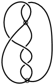
Figure 12. The virtual knot $K=4.41$.

Corollary 5.4.

If $K$ is a mod $p$ almost classical knot or link and $\zeta$ is a non-trivial $p$-th root of unity, then $\hbox{ \kern 0.09995pt\vbox{\hrule height=0.5pt\kern 1.07639pt\hbox{\kern-1.99997pt$H$\kern-0.50003pt}}\kern-0.29999pt}_{K}(t,\zeta)=0$. If $K$ is almost classical, then $\hbox{ \kern 0.09995pt\vbox{\hrule height=0.5pt\kern 1.07639pt\hbox{\kern-1.99997pt$H$\kern-0.50003pt}}\kern-0.29999pt}_{K}(t,v)=0.$

Remark 5.5.

The same result holds for twisted virtual Alexander polynomials $\hbox{ \kern 0.09995pt\vbox{\hrule height=0.5pt\kern 1.07639pt\hbox{\kern-1.99997pt$H$\kern-0.50003pt}}\kern-0.29999pt}^{\varrho}(t,v)$; if $K$ is a mod $p$ almost classical knot or link and $\varrho\colon\operatorname{\it\hbox{ \kern 0.09995pt\vbox{\hrule height=0.5pt\kern 1.07639pt\hbox{\kern-1.99997pt$G$\kern-0.50003pt}}\kern-0.29999pt}}_{K}\to GL_{n}(R)$, then $\hbox{ \kern 0.09995pt\vbox{\hrule height=0.5pt\kern 1.07639pt\hbox{\kern-1.99997pt$H$\kern-0.50003pt}}\kern-0.29999pt}^{\varrho}(t,\zeta)=0$ for any non-trivial $p$-th root of unity $\zeta$. If $K$ is almost classical, then $\hbox{ \kern 0.09995pt\vbox{\hrule height=0.5pt\kern 1.07639pt\hbox{\kern-1.99997pt$H$\kern-0.50003pt}}\kern-0.29999pt}^{\varrho}_{K}(t,v)=0.$

Proof.

Let $\operatorname{\it\hbox{ \kern 0.09995pt\vbox{\hrule height=0.5pt\kern 1.07639pt\hbox{\kern-1.99997pt$G$\kern-0.50003pt}}\kern-0.29999pt}}_{K}=\langle a_{1},\ldots,a_{n},v\mid r_{1},\ldots,r_{n}\rangle$. Then the $n\times(n+1)$ presentation matrix for the Alexander module of $\operatorname{\it\hbox{ \kern 0.09995pt\vbox{\hrule height=0.5pt\kern 1.07639pt\hbox{\kern-1.99997pt$G$\kern-0.50003pt}}\kern-0.29999pt}}_{K}$ is given by

$$\begin{bmatrix}A&\left(\frac{\partial r}{\partial v}\right)\end{bmatrix},$$

where $A=\left(\left.\frac{\partial r_{i}}{\partial a_{j}}\right|_{a_{1},\ldots,a_{n}=t}\right)$ is the $n\times n$ meridional Alexander matrix and $\left(\frac{\partial r}{\partial v}\right)$ is the column vector whose $i$-th entry is $\left.\frac{\partial r_{i}}{\partial v}\right|_{a_{1},\ldots,a_{n}=t}$. By the fundamental identity of Fox derivatives, it follows that $\hbox{ \kern 0.09995pt\vbox{\hrule height=0.5pt\kern 1.07639pt\hbox{\kern-1.99997pt$H$\kern-0.50003pt}}\kern-0.29999pt}_{K}(t,v)=\det A$.

The result will be established by relating $\hbox{ \kern 0.09995pt\vbox{\hrule height=0.5pt\kern 1.07639pt\hbox{\kern-1.99997pt$H$\kern-0.50003pt}}\kern-0.29999pt}_{K}(t,v)$ to the first elementary ideal associated to the quotient group $\operatorname{\it\hbox{ \kern 0.09995pt\vbox{\hrule height=0.5pt\kern 1.07639pt\hbox{\kern-1.99997pt$G$\kern-0.50003pt}}\kern-0.29999pt}}_{K}/\langle v^{p}\rangle=\langle a_{1},\ldots,a_{n},v\mid r_{1},\ldots,r_{n},v^{p}\rangle$. Its Alexander module has $(n+1)\times(n+1)$ presentation matrix given by

$$M=\begin{bmatrix}\,A&\left(\frac{\partial r}{\partial v}\right)\\[5.0pt] 0&\sum_{k=0}^{p-1}v^{k}\end{bmatrix}.$$

Its first elementary ideal is the ideal generated by all the $n\times n$ minors of $M$, and in particular its Alexander polynomial $\Delta^{1}(t,v)$ is given by the $\gcd$ of all these minors. Since $\det A$ is among the minors, it follows that $\Delta^{1}(t,v)$ divides $\det A=\hbox{ \kern 0.09995pt\vbox{\hrule height=0.5pt\kern 1.07639pt\hbox{\kern-1.99997pt$H$\kern-0.50003pt}}\kern-0.29999pt}_{K}(t,v)$.

If $K$ is mod $p$ almost classical, then by Theorem 5.2, the quotient group admits a presentation of the form

$$\operatorname{\it\hbox{ \kern 0.09995pt\vbox{\hrule height=0.5pt\kern 1.07639pt\hbox{\kern-1.99997pt$G$\kern-0.50003pt}}\kern-0.29999pt}}_{K}/\langle v^{p}\rangle\cong G_{K}*{\mathbb{Z}}/p=\langle a_{1},\ldots,a_{n},v\mid r_{1},\ldots,r_{n},v^{p}\rangle,$$

where the relations $r_{1},\ldots,r_{n}$ are independent of $v.$ The associated presentation matrix for the Alexander module is then given by

$$M^{\prime}=\begin{bmatrix}\,A&0\\[3.00003pt] 0&\sum_{k=0}^{p-1}v^{k}\end{bmatrix},$$

where $A$ is now the Alexander matrix for $G_{K}$. The fundamental identity of Fox derivatives implies that $\det A=0$. Notice that the term $\sum_{k=0}^{p-1}v^{k}$ appears in each of the other $n\times n$ minors of $M^{\prime},$ and this shows that $\sum_{k=0}^{p-1}v^{k}$ divides $\Delta^{1}(t,v)$, so it must also divide $\hbox{ \kern 0.09995pt\vbox{\hrule height=0.5pt\kern 1.07639pt\hbox{\kern-1.99997pt$H$\kern-0.50003pt}}\kern-0.29999pt}_{K}(t,v)$. We conclude that $\hbox{ \kern 0.09995pt\vbox{\hrule height=0.5pt\kern 1.07639pt\hbox{\kern-1.99997pt$H$\kern-0.50003pt}}\kern-0.29999pt}_{K}(t,\zeta)=0$ if $\zeta$ is a non-trivial $p$-th root of unity. ∎

Combining Theorem 4.1 and Corollary 5.4 yields the following divisibility property of the generalized Alexander polynomial $G_{K}(s,t)$.

Proposition 5.6.

If $K$ is a mod $p$ almost classical knot or link then the $p$-th cyclotomic polynomial $\Phi_{p}(s)$ divides $G_{K}(s,t)$.∎

For example, consider the virtual knots $4.91$ and $4.92$ from the virtual knot table of Green [15]. The virtual knot $K=4.91$ has generalized Alexander polynomial

$$G_{K}(s,t)=(s-1)(t-1)(st-1)(s^{2}t^{2}+st^{2}+s^{2}t+t^{2}+2st+s^{2}+t+s+1).$$

Since $G_{K}(s,t)$ is not divisible by any cyclotomic polynomial in $s$, we conclude that $K=4.91$ is not mod p almost classical for any $p$.

On the other hand, the virtual knot $K=4.92$ has generalized Alexander polynomial

$$G_{K}(s,t)=(s-1)(t-1)(st-1)(s^{2}+s+1)(t^{2}+t+1),$$

which is divisible by $s^{2}+s+1$. One can easily check that $K=4.92$ is mod 3 Alexander numberable.

6. Seifert surfaces for almost classical knots

In this section, we give a construction of the Seifert surface $F$ associated to an almost classical knot or link $K$. Our construction is modelled on Seifert’s algorithm. In the following section, we will use the Seifert surface to show that the first elementary ideal $\mathcal{E}_{1}$ is principal.

Theorem 6.1.

For a virtual knot or link $K$, the following are equivalent.

• $K$ is almost classical, i.e., some virtual knot diagram for $K$ admits an Alexander numbering.

• $K$ is homologically trivial as a knot or link in $\Sigma\times[0,1]$, where $\Sigma$ is the Carter surface associated to an Alexander numberable diagram of $K$.

• $K$ is the boundary of a connected, oriented surface $F$ embedded in $\Sigma\times[0,1]$, where $\Sigma$ is again the Carter surface associated to an Alexander numberable diagram of $K$.

The surface $F$ from part (c) is called a Seifert surface for $K$.

The argument that (a) $\Leftrightarrow$ (b) was given in Section 5. If $K=\partial F$ for an oriented surface $F\hookrightarrow\Sigma\times[0,1]$, then $K$ is necessarily homologically trivial. Thus (c) $\Rightarrow$ (b). On the other hand, it is well known that an oriented, null homologous link in an oriented 3-manifold admits a Seifert surface (see [10, Lemma 2.2] or [29, Proposition 27.5]). This section is devoted to providing an explicit algorithm for constructing the Seifert surface of an almost classical knot or link, and this will show that (b) $\Rightarrow$ (c) and complete the proof of the theorem.

We begin by recalling Seifert’s algorithm. If $K$ is a classical knot, after smoothing all the crossings, we obtain a disjoint collection of oriented simple closed curves called Seifert circuits. Each Seifert circuit bounds a 2-disk in the plane, and the resulting system of 2-disks may be nested in ${\mathbb{R}}^{2}$, but we can put them at different levels in ${\mathbb{R}}^{3}$ and thus arrange them to be disjoint. The Seifert surface $F$ is then built from the disjoint union $D_{1}\cup\cdots\cup D_{n}$ of Seifert disks by attaching half-twisted bands at each crossing.

A slight modification of this procedure enables us to construct Seifert surfaces for homologically trivial knots $K$ in $\Sigma\times[0,1]$. First smooth the crossings of $K$ to obtain a collection $\gamma_{1},\ldots,\gamma_{n}$ of oriented disjoint simple closed curves in $\Sigma\times[0,1]$. Since $K$ is homologically trivial, it follows that $\sum_{i}[\gamma_{i}]=0$ in $H_{1}(\Sigma;{\mathbb{Z}})$.

Proposition 6.2.

If $\gamma_{1},\ldots,\gamma_{n}$ are disjoint oriented simple closed curves in an oriented surface $\Sigma$ whose union is homologically trivial, then there exists a collection $S_{1},\ldots,S_{m}$ of connected oriented subsurfaces of $\Sigma$ such that

$$\bigcup_{j=1}^{m}\partial S_{j}=\bigcup_{i=1}^{n}\gamma_{i}.$$

The orientation of each $S_{j}$ may or may not agree with the orientation of $\Sigma$, and the boundary orientation on $\partial S_{j}$ is the one induced by the outward normal first convention.

We can assume that $S_{j}$ has nonempty boundary $\partial S_{j}$ for each $j$, though we do not assume that $\partial S_{j}$ is connected. The subsurfaces may have nonempty intersection $S_{i}\cap S_{j}$, but their boundaries $\partial S_{1},\ldots,\partial S_{m}$ are necessarily disjoint (since $\gamma_{1},\ldots,\gamma_{n}$ are).

The subsurfaces $S_{j}$ are the building blocks for the Seifert surface and in fact, given Proposition 6.2 one can easily construct the Seifert surface $F$ for $K$ as follows. By placing $S_{1},\ldots,S_{m}$ at different levels in the thickened surface $\Sigma\times[0,1]$, we can arrange them to be disjoint. We then glue in small half-twisted bands at each crossing of $K$, and the result is an oriented surface $F$ embedded in $\Sigma\times[0,1]$ with $\partial F=K$.

We now complete the argument by proving the proposition.

Proof.

The proof is by induction on $n,$ and the base case $n=1$ amounts to the observation that a single curve $\gamma_{1}$ is homologically trivial if and only if it is a separating curve on $\Sigma$. In fact, the Alexander numbering of $\gamma_{1}$ induces an Alexander numbering of $\Sigma\smallsetminus\gamma_{1}$ with the region to the left of $\gamma_{1}$ having number $\lambda_{1}-1$ and the region to the right having number $\lambda_{1}$. Thus $\Sigma\smallsetminus\gamma_{1}$ is disconnected, and one can take $S_{1}$ to be either of the oriented subsurfaces of $\Sigma$ bounding $\gamma_{1}$.

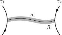
Figure 13. Two curves $\gamma_{1}$ and $\gamma_{2}$, and a path $\alpha$ connecting them. The thin rectangle $R$ is the shaded region, and in this figure the orientations of $\gamma_{1}$ and $\gamma_{2}$ are consistent with that of $R$.

Now suppose $n=2.$ If $\gamma_{1}$ is separating, then we again have a subsurface $S_{1}$ with $\partial S_{1}=\gamma_{1}$, and we are reduced to the previous case. If instead $\gamma_{1}$ and $\gamma_{2}$ are both non-separating, we choose a path $\alpha\colon[0,1]\to\Sigma$ from $\gamma_{1}$ to $\gamma_{2}$. We can assume that, apart from its endpoints, the path $\alpha$ does not intersect $\gamma_{1}$ or $\gamma_{2}.$ Thicken $\alpha$ slightly to get a long thin rectangle $R$ embedded in $\Sigma$ with short sides along $\gamma_{1}$ and $\gamma_{2}.$ Orient $R$ so that its boundary orientation is consistent with $\gamma_{1}$ on the short side along $\gamma_{1}$. Then we claim that the orientation of $R$ on the other short side along $\gamma_{2}$ is consistent with $\gamma_{2}.$ We prove this by contradiction using the Alexander numbering. If the orientation is not consistent, then the regions of $\Sigma\smallsetminus(\gamma_{1}\cup\gamma_{2})$ would require three different Alexander numbers, implying that $\Sigma\smallsetminus(\gamma_{1}\cup\gamma_{2})$ has at least three components, which contradicts the assumption that $\gamma_{1}$ is non-separating.

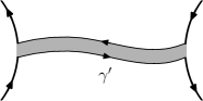
Figure 14. The curve $\gamma^{\prime}$ is homologous to $\gamma_{1}\cup\gamma_{2}$.

Thus, the orientations of $\gamma_{1}$ and $\gamma_{2}$ are both consistent with the rectangle $R$, and we replace $\gamma_{1}\cup\gamma_{2}$ with a single curve $\gamma^{\prime}$ homologous to $\gamma_{1}\cup\gamma_{2}$. Since $\gamma^{\prime}$ is null homologous, it is separating and that gives a subsurface $S$ of $\Sigma$ with $\partial S=\gamma^{\prime}$. We now perform surgery on $S$ to obtain the desired subsurface $S^{\prime}$ with $\partial S^{\prime}=\gamma_{1}\cup\gamma_{2}.$ Before describing the surgery operation, notice that due to boundary considerations, either $R$ is contained entirely in $S$ or they intersect only along the (long) edges of $R$. The surgery operation amounts to removing $R$ from $S$ in the first case, or pasting $R$ into $S$ in the second. In the boundary, this amounts to replacing the long edges of $R$ with the short edges, and thus $\partial S^{\prime}=\gamma_{1}\cup\gamma_{2}.$

The inductive step follows by a similar argument. If any one of $\gamma_{1},\ldots,\gamma_{n}$ is separating, then we have a subsurface $S_{1}$ bounding it and we can reduce to the case of $n-1$ null-homologous curves. On the other hand, if each $\gamma_{i}$ is non-separating, then we claim we can find a pair of them, say $\gamma_{1}$ and $\gamma_{2}$, together with an arc $\alpha$ connecting them so that, the long thin rectangle $R$ we get from thickening $\alpha$ can be oriented consistently with $\gamma_{1}$ and $\gamma_{2}.$ Once that is established, we replace $\gamma_{1}\cup\gamma_{2}$ by $\gamma^{\prime}$ as before and apply induction to the $n-1$ curves $\gamma^{\prime},\gamma_{3},\ldots,\gamma_{n}$.

It remains to be seen that the path $\alpha$ can be chosen so the orientations of $\gamma_{1}$ and $\gamma_{2}$ are consistent with the rectangle $R$ formed by thickening $\alpha$. To that end, choose a basepoint $p\in\gamma_{1}$ and push-offs $p_{+}$ and $p_{-}$ in $\Sigma\smallsetminus\gamma_{1}$ to the right and to the left of $p.$ Since $\gamma_{1}$ is non-separating, we have a path $\alpha$ in $\Sigma\smallsetminus\gamma_{1}$ connecting $p_{+}$ to $p_{-}$. Notice that the Alexander numbers of $p_{+}$ and $p_{-}$ are not equal. Notice further that the Alexander number of any point on $\alpha$ is constant except when $\alpha$ crosses one of the other curves $\gamma_{2},\ldots,\gamma_{n}.$ We can assume $\alpha$ intersects each $\gamma_{i}$ transversely. We can also assume, by relabeling, that the first curve $\alpha$ intersects is $\gamma_{2}.$ If $\gamma_{1}$ and $\gamma_{2}$ are oriented consistently, then we can replace the pair $\gamma_{1}\cup\gamma_{2}$ by $\gamma^{\prime}$ as before and apply induction to $\gamma^{\prime},\gamma_{3},\ldots,\gamma_{n}$. Otherwise, we notice that the Alexander number of $\alpha$ must increase as it crosses $\gamma_{2}.$ Continue in this manner, since the Alexander number of $p_{-}$ is one less than that of $p_{+},$ eventually we must encounter a curve $\gamma_{i}$ where the Alexander number of $\alpha$ decreases. One can verify that this curve and the previous one are consistently oriented, and using the segment of $\alpha$ connecting them one can form $\gamma^{\prime}$, reduce to the case of $n-1$ curves and apply induction. This produces a collection of subsurfaces whose boundary is the new set of curves, and the subsurfaces can again be modified by performing surgery, i.e. by either adding or removing the rectangle $R$, and this gives a collection of subsurfaces with boundary $\gamma_{1}\cup\cdots\cup\gamma_{n}$. ∎

Definition 6.3.

The Seifert genus of an almost classical knot or link $K$, denoted $g_{s}(K)$, is defined to be the minimum genus over all connected, oriented surfaces $F\hookrightarrow\Sigma\times[0,1]$ with $K=\partial F$ and over all Alexander numberable diagrams for $K$.

The next result shows that the genus of a Seifert surface is monotonically non-increasing under destabilization.

Theorem 6.4.

Let $K$ be homologically trivial knot in a thickened surface $\Sigma\times I$ with Seifert surface $F$. Suppose $A$ is a vertical annulus in $\Sigma\times I$ disjoint from $K$, and let $\Sigma^{\prime}$ be the surface obtained from $\Sigma$ by destabilization along $A$. (If destabilization along $A$ separates $\Sigma$, we choose $\Sigma^{\prime}$ to be the component containing $K$.) Then there exists a Seifert surface $F^{\prime}$ in $\Sigma^{\prime}\times I$ for $K$ with $g(F^{\prime})\leq g(F).$

Proof.

Given a vertical annulus $A$ for $\Sigma\times I$, consider its intersection $F\cap A$ with the Seifert surface $F$. If $F\cap A$ is empty, then $F$ is a surface in $\Sigma^{\prime}\times I$ and taking $F^{\prime}=F$ satisfies the statement of the theorem. If on the other hand $F\cap A$ is non-empty, then it must consist of a union of circles, possibly nested, in $A$. The idea is to perform surgery on the circles, one at a time, working from an innermost circle. (Innermost circles exist but are not necessarily unique.)

Let $C$ denote such a circle. Viewing $C$ in $F$, then either it is a separating curve or a non-separating curve. If it’s separating, then we can perform surgery to $F$ along $C$ in $\Sigma^{\prime}\times I$ and $F$ will split into a disjoint union $F^{\prime}\cup F^{\prime\prime},$ with $F^{\prime\prime}$ a closed surface and with $\partial F^{\prime}=K$. Clearly $F^{\prime}$ is a surface in $\Sigma^{\prime}\times I$ and $g(F^{\prime})\leq g(F)$ as claimed.

Otherwise, if the circle is non-separating in $F$, then using it to perform surgery to $F$, we obtain a Seifert surface $F^{\prime}$ for $K$ in $\Sigma^{\prime}\times I$ and $g(F^{\prime})=g(F)-1.$ ∎

Recall that for a virtual knot $K$, the virtual genus of $K$ is the minimal genus over all thickened surfaces $\Sigma\times I$ in which $K$ can be realized. The next result is a direct consequence of Theorem 6.4, and it shows that a Seifert surface of minimal genus for an almost classical knot $K$ can always be constructed in the thickened surface $\Sigma\times I$ of minimal genus.

Corollary 6.5.

If $K$ is an almost classical knot with virtual genus $h$, then there exists a Seifert surface $F$ of minimal genus in the thickened surface $\Sigma\times I$ of genus $g(\Sigma)=h.$

7. Alexander polynomials for almost classical knots

In this section, we extend various classical results to the almost classical setting by using the Seifert surface constructed in the previous section. Recall that for a classical knot $K$ in $S^{3}$, the Alexander module can be viewed as the first homology of the infinite cyclic cover $X_{\infty}$, which can be constructed by cutting the complement $S^{3}\smallsetminus K$ along a Seifert surface and gluing countably many copies end-to-end (cf. [22, Ch. 6]).

We begin this section by performing a similar construction for almost classical knots $K$, and we use this approach to define Seifert forms $\alpha^{\pm}$ and Seifert matrices $V^{\pm}$, which we show give a presentation for the first elementary ideal $\mathcal{E}_{1}$ of the Alexander module. It follows that $\mathcal{E}_{1}$ is principal when $K$ is an almost classical knot or link, and this recovers and extends the principality result in [28]. We then define the Alexander polynomial of an almost classical knot or link $K$ to be the polynomial $\Delta_{K}(t)=\det(tV^{-}-V^{+})\in{\mathbb{Z}}[t^{\pm 1}]$ with $\mathcal{E}_{1}=(\Delta_{K}(t))$, which is well-defined up to multiplication by $t^{g}$ where $g$ is the virtual genus of $K$. (This is an improvement, for instance Lemma 7.5 allows us to remove the sign ambiguity that one would have if one simply defined $\Delta_{K}(t)$ as a generator of the principal ideal $\mathcal{E}_{1}$.)

We give a bound on the Seifert genus $g_{s}(K)$ in terms of $\deg\Delta_{K}(t)$ and prove that $\Delta_{K}(t)$ is multiplicative under connected sum of almost classical knots. We establish a skein formula for $\Delta_{K}(t)$ and extend the knot determinant to the almost classical setting by taking $\det(K)=|\Delta_{K}(-1)|$, which we show is odd for almost classical knots. We briefly explore to what extent these results can be extended to mod $p$ almost classical knots and links.

We begin by recalling the definition of linking number, $\operatorname{\ell{\it k}}(J,K)$ for a pair $(J,K)$ of disjoint oriented knots in $\Sigma\times I$.

Proposition 7.1.

The relative homology group $H_{1}(\Sigma\times I\smallsetminus J,\,\Sigma\times 1)$ is infinite cyclic generated by a meridian $\mu$ of $J$.

Proof.

We apply the Mayer-Vietoris sequence to the union $\Sigma\times I=(\Sigma\times I\smallsetminus J)~{}\cup~{}\operatorname{int}(N(J)),$ where $N(J)$ is a closed regular neighborhood of $J$. Let $j\colon\Sigma\to\Sigma\times I\smallsetminus J$ be given by $j(x)=(x,1)$, let $i\colon\Sigma\times I\smallsetminus J\to\Sigma\times I$ be inclusion and let $p\colon\Sigma\times I\to\Sigma$ be projection. The composite

$$\Sigma~{}\stackrel{{\scriptstyle j}}{{\longrightarrow}}~{}\Sigma\times I\smallsetminus J~{}\stackrel{{\scriptstyle i}}{{\longrightarrow}}~{}\Sigma\times I~{}\stackrel{{\scriptstyle p}}{{\longrightarrow}}\Sigma$$

is the identity and hence $i_{*}\colon H_{*}(\Sigma\times I\smallsetminus J)\to H_{*}(\Sigma\times I)$ is a split surjection and $j_{*}\colon H_{*}(\Sigma)\to H_{*}(\Sigma\times I\smallsetminus J)$ is a split injection and thus the Mayer-Vietoris sequence yields the short exact sequence

$$0\to H_{1}\left(\partial N(J)\right)~{}\to~{}H_{1}(\Sigma\times I\smallsetminus J)\oplus H_{1}(J)~{}\to~{}H_{1}(\Sigma\times I)\to 0,$$

moreover, $H_{1}\left(\partial N(J)\right)\cong{\mathbb{Z}}\oplus{\mathbb{Z}}$, generated by a meridian and longitude of $J$, and the summand generated by the longitude maps isomorphically to $H_{1}(J)\cong{\mathbb{Z}}$. The exact sequence of the pair $\left(\Sigma\times I\smallsetminus J,\,\Sigma\times 1\right)$ yields the split short exact sequence

$$0\to H_{1}\left(\Sigma\times 1\right)~{}\to~{}H_{1}(\Sigma\times I\smallsetminus J)~{}\to~{}H_{1}(\Sigma\times I\smallsetminus J,\,\Sigma\times 1)\to 0.$$

Combining the above two short exact sequences yields the conclusion. ∎

The knot $K$ determines a homology class $[K]$ in $H_{1}(\Sigma\times I\,\smallsetminus J,\,\Sigma\times 1)$ and $\operatorname{\ell{\it k}}(J,K)$ is the unique integer $m$ such that $[K]=m\mu$. A geometric description of the linking number is given as follows. Let $B$ be a $2$-chain in $\Sigma\times I$ such that $\partial B=K-v$, where $v$ is a $1$-cycle in $\Sigma\times 1\subset\Sigma\times I$. Then $\operatorname{\ell{\it k}}(J,K)=J\cdot B$ (the homological intersection number of $J$ with $B$), see [10, §1.2]. Note that $\operatorname{\ell{\it k}}(K,J)-\operatorname{\ell{\it k}}(J,K)=p_{*}([J])\cdot p_{*}([K])$, where $p_{*}([J])\cdot p_{*}([K])$ is the intersection number in $\Sigma$ of the projections of $J$ and $K$ to $\Sigma$, [10, §1.2], and so the linking number need not be symmetric.

Let $F$ be a compact, connected oriented surface of genus $g$ with $n$ boundary components, $n>0$, embedded in the interior of $\Sigma\times I$. The homology groups $H_{1}(\Sigma\times I\,\smallsetminus F,\,\Sigma\times 1)$ and $H_{1}(F)$ are isomorphic, both are free abelian of rank $2g+n-1$, and, furthermore, there is a unique non-singular bilinear form

$$\beta\colon H_{1}(\Sigma\times I\,\smallsetminus F,\,\Sigma\times 1)~{}\times~{}H_{1}(F)~{}\longrightarrow~{}{\mathbb{Z}}$$

such that $\beta([c],[d])=\operatorname{\ell{\it k}}(c,d)$ for all oriented closed simple curves $c$ and $d$ in $\Sigma\times I\smallsetminus F$ and $F$, respectively. The proof of this assertion is similar to the classical case (that is, $S^{3}$ in place of $\Sigma\times I$) as given in [22, Proposition 6.3] and makes use of an analysis of the Mayer-Vietoris sequence of the union $\Sigma\times I=(\Sigma\times I\smallsetminus F)~{}\cup~{}\operatorname{int}(N(F))$, where $N(F)$ is a closed regular neighborhood of $F$.

Assume that $F$ is a connected Seifert surface for a homologically trivial oriented link $L$ with $n$ components in $\Sigma\times I$. The surface $F$ has a closed regular neighborhood $N(F)$ that can be given a parametrization $F\times[-1,1]\cong N(F)$ with $F\times 0$ corresponding to $F$ and such that the meridian of each component of $L$ enters $N(F)$ at $F\times-1$ and departs at $F\times 1$. Let $\iota^{\pm}\colon F\to\Sigma\times I\smallsetminus F$ be the embeddings given by $\iota^{\pm}(x)=(x,\,\pm 1)$, and we denote by $x^{\pm}=\iota^{\pm}(x)$ the “positive and negative pushoffs”. We thus obtain a pair of bilinear forms, the Seifert forms of $F$,

$$\alpha^{\pm}\colon H_{1}(F)~{}\times~{}H_{1}(F)~{}\longrightarrow~{}{\mathbb{Z}}$$

given by $\alpha^{\pm}(x,y)=\beta(x^{\pm},y)$.

Let $Z=\left(\Sigma\times I\,\smallsetminus L\right)/\,\Sigma\times 1$ be the space obtained from $\Sigma\times I\,\smallsetminus L$ by collapsing $\Sigma\times 1$ to a point. The fundamental group of $Z$ is isomorphic to the link group $G_{L}$. The abelianization of $G_{L}$ is $H_{1}(G_{L})\cong H_{1}(Z)\cong H_{1}(\Sigma\times I\,\smallsetminus L,\,\Sigma\times 1)\cong{\mathbb{Z}}^{n}$. Let $\varepsilon\colon{\mathbb{Z}}^{n}\to{\mathbb{Z}}$ be the homomorphism $\varepsilon(a_{1},\ldots,a_{n})=\sum^{n}_{i=1}a_{i}$ and let $Z_{\infty}$ be the covering space of $Z$ corresponding to the homomorphism $G_{L}\to H_{1}(G_{L})\cong{\mathbb{Z}}^{n}\stackrel{{\scriptstyle\varepsilon}}{{\longrightarrow}}{\mathbb{Z}}$. We construct a model for $Z_{\infty}$, generalizing the well-known construction in [22, §6], using the Seifert surface $F$ together with the parametrization $F\times[-1,1]\cong N(F)$. Let $X=\left(\Sigma\times I\,\smallsetminus\operatorname{int}(N(F))\right)/\,\Sigma\times 1$. Note that $X$ is a finite CW complex and $H_{1}(X)\cong H_{1}(\Sigma\times I\,\smallsetminus F,\,\Sigma\times 1)$. Let $Y$ be the space obtained by cutting $X$ along $F$, that is, $Y$ is up to homeomorphism the space $X\smallsetminus F$ compactified with two copies, $\iota^{-}(F)$ and $\iota^{+}(F)$, of $F$. Let $\varphi\colon\iota^{-}(F)\to\iota^{+}(F)$ be the homeomorphism determined by $\iota^{\pm}$. (Note that $X$ can be recovered from $Y$ by identifying $\iota^{-}(F)$ with $\iota^{+}(F)$ via $\varphi$.) Set $Y_{i}=Y\times\{i\}$ for $i\in{\mathbb{Z}}$ and let $X_{\infty}$ be the space obtained from the disjoint union $\bigcup_{i\in{\mathbb{Z}}}Y_{i}$ by gluing $Y_{i}$ to $Y_{i+1}$ by identifying $F_{i}^{-}=\iota^{-}(F)\times\{i\}$ to $F_{i+1}^{+}=\iota^{+}(F)\times\{i+1\}$ via $\varphi.$ In other words, $(y^{-},i)\sim(\varphi(y)^{+},i+1)$ for $y\in F$, where $y^{\pm}=\iota^{\pm}(y)$ denote the positive and negative push-offs. Then $X_{\infty}$ is homeomorphic to the infinite cyclic cover $Z_{\infty}$, and the homeomorphism $t\colon X_{\infty}\to X_{\infty}$ given by $t(y,i)=(y,i+1)$ induces an isomorphism $t\colon H_{1}(X_{\infty})\longrightarrow H_{1}(X_{\infty})$ and gives $H_{1}(X_{\infty})$ the structure of a ${\mathbb{Z}}[t^{\pm 1}]$-module. The argument employed in [22, Theorem 6.5] extends to prove the following theorem.

Theorem 7.2.

Let $F$ be a connected Seifert surface for a homologically trivial oriented link $L$ in $\Sigma\times I$. Let $V^{\pm}$ be matrices for the Seifert forms $\alpha^{\pm}$ with respect to a given basis for $H_{1}(F)$. Then $t\,V^{-}-\,V^{+}$ is a presentation matrix for the ${\mathbb{Z}}[t^{\pm 1}]$-module $H_{1}(X_{\infty})$. ∎

Corollary 7.3.

The first elementary ideal of an almost classical knot or link $L$ is principal, generated by $\det(tV^{-}-V^{+})$ with $V^{\pm}$ as in Theorem 7.2. Hence, up to units, $\Delta_{L}(t)$ coincides with $\det(tV^{-}-V^{+})$.

Remark 7.4.

Note that for a classical link, the matrices $V^{-}$ and $V^{+}$ are transposes of each other. This need not be true if the genus of $\Sigma$ is positive. Theorem 7.2 shows that our $\Delta_{L}(t)$ coincides (up to units) with the extended Alexander-Conway polynomial of $L$ as defined by Cimasoni and Turaev, [10].

The next result is standard, and for a proof see Lemma 6.7.6 of [11].

Lemma 7.5.

Suppose $L$ is an almost classical knot or link with $n$ components. Then

$$\det(V^{-}-V^{+})=\begin{cases}1&\text{if $\,n=1$,}\\ 0&\text{if $\,n>1.$ }\end{cases}$$

Definition 7.6.

If $K$ is an almost classical knot or link, we define its Alexander polynomial to be the Laurent polynomial $\Delta_{K}(t)=\det(tV^{-}-V^{+})$. Theorem 7.2 shows that $\Delta_{K}(t)$ is a generator of the first elementary ideal $\mathcal{E}_{1},$ and Lemma 7.5 shows that $\Delta_{K}(1)=1$ for knots and that $\Delta_{K}(1)=0$ for links. As an invariant of almost classical knots and links, $\Delta_{K}(t)$ is well-defined up to units in ${\mathbb{Z}}[t^{\pm 1}],$ and it is an invariant of the welded equivalence class of $K$.

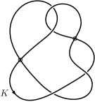
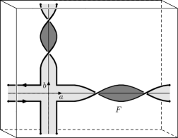
Figure 15. The virtual knot $4.99$ on the left and its Seifert surface in $T^{2}\times I$ on the right.

Example 7.7.

The Carter surface $\Sigma_{K}$ of the virtual knot $K=4.99$ has genus $g(\Sigma_{K})=1$ and Figure 15 shows a virtual knot diagram for $K$ along with its Seifert surface $F\subset T^{2}\times I.$ (In Figure 15, $T^{2}\times I$ is obtained from the cube on the right by identifying the two faces on top and bottom and the two faces on left and right in the obvious way. The front face is $T^{2}\times 1$, and this choice determines how to compute linking numbers.)

This shows that $F$ is a union of two twisted bands and also has genus $g(F)=1.$ We will use Figure 15 to compute the Seifert matrices $V^{\pm}$ of $F$ in terms of the generators $a,b\in H_{1}(F)$. We orient $F$ so that $a\cdot b=1$, and we orient $F\times[-1,1]$ so that $a^{+}$ and $b^{+}$ are obtained by pushing up along the darker region and down along the lighter region. Using the picture, one can see that

$$\operatorname{\ell{\it k}}(a^{+},a)=-1, \operatorname{\ell{\it k}}(a^{+},b)=0,$$

$$\operatorname{\ell{\it k}}(b^{+},a)=0, \operatorname{\ell{\it k}}(b^{+},b)=1,$$

and that implies $V^{+}=\begin{bmatrix}-1&0\\ 0&1\end{bmatrix}.$ Similarly, we have

$$\operatorname{\ell{\it k}}(a^{-},a)=-1 \operatorname{\ell{\it k}}(a^{-},b)=1$$

$$\operatorname{\ell{\it k}}(b^{-},a)=-1 \operatorname{\ell{\it k}}(b^{-},b)=1$$

which implies $V^{-}=\begin{bmatrix}-1&1\\ -1&1\end{bmatrix}.$ Thus

$$\Delta_{K}(t)=\det\left(tV^{-}-V^{+}\right)=\det\left(\begin{bmatrix}1-t&t\\ -t&t-1\end{bmatrix}\right)=2t-1.$$

Remark 7.8.

Taking $\Delta_{K}(t)=\det\left(t^{1/2}V^{-}-t^{-1/2}V^{+}\right)$ gives a normalization (Conway polynomial) that is well-defined up to multiplication by $t^{g}$, where $g=g(\Sigma_{K})$ is the genus of the minimal Carter surface. This follows by combining the argument on p. 560 of [10] with the statement of Kuperberg’s theorem [21]. In the example above, since $g(\Sigma_{K})=1,$ this means that $\Delta_{K}(t)$ has a well-defined sign determined by Lemma 7.5.

For the Laurent polynomial $f(t)$, we define $0pt(f(t))$ as the difference between its top degree and its lowest degree. The next result shows that the Seifert genus is bounded below by the width of $\Delta_{K}(t)$.

Theorem 7.9.

Suppose $K$ is an almost classical knot or link with $n$ components, then

$$0pt\Delta_{K}(t)~{}\leq~{}2g_{s}(K)+n-1.$$

Proof.

Given a Seifert surface $F$ for $K$, we see that $H_{1}(F)$ is free abelian of rank $2g(F)+n-1$. Thus the Seifert matrices $V^{+}$ and $V^{-}$ are square matrices of size $2g(F)+n-1$, and it follows that

$$0pt\Delta_{K}(t)\leq\deg\left(\det(tV^{-}-V^{+})\right)\leq 2g(F)+n-1.$$

Taking a Seifert surface $F$ of minimal genus, we have $g_{s}(K)=g(F)$ and the theorem now follows. ∎

The next result shows that the Alexander polynomial $\Delta_{K}(t)$ is multiplicative under connected sum. Note that although connected sum is not a well-defined procedure for virtual knots, it is nevertheless true that if $K_{1}$ and $K_{2}$ are both Alexander numberable diagrams, then so is $K_{1}\#K_{2}$ for all possible choices, and the Alexander polynomial of $K_{1}\#K_{2}$ is independent of these choices.

Theorem 7.10.

If $K_{1}$ and $K_{2}$ are both Alexander numberable, then so is $K_{1}\#K_{2}$, and $\Delta_{K_{1}\#K_{2}}(t)=\Delta_{K_{1}}(t)\,\Delta_{K_{2}}(t).$

Proof.

Let $\Sigma_{1}$ and $\Sigma_{2}$ be the Carter surfaces for $K_{1}$ and $K_{2},$ respectively, and construct Seifert surfaces $F_{1}\subset\Sigma_{1}\times I$ and $F_{2}\subset\Sigma_{2}\times I.$ Thus the knot $K_{1}\#K_{2}$ has Carter surface $\Sigma_{1}\#\Sigma_{2},$ and the boundary connected sum of $F_{1}$ and $F_{2}$ is a Seifert surface for $K_{1}\#K_{2}$. Theorem 6.1 applies to show that $K_{1}\#K_{2}$ is almost classical, and the Seifert matrices of the surface $F_{1}\#F_{2}$ are easily seen to be block diagonal. Thus

$$V^{\pm}=\begin{bmatrix}V^{\pm}_{1}&0\\ 0&V^{\pm}_{2}\end{bmatrix},$$

where $V^{\pm}_{1}$ and $V^{\pm}_{2}$ denote the Seifert matrices of $F_{1}$ and $F_{2},$ respectively. It follows that

$$\Delta_{K_{1}\#K_{2}}(t) = \det\left(tV^{-}-V^{+}\right)$$

$$= \det\left(\begin{bmatrix}tV^{-}_{1}-V^{+}_{1}&0\\ 0&tV^{-}_{2}-V^{+}_{2}\end{bmatrix}\right)$$

$$= \det\left(tV^{-}_{1}-V^{+}_{1}\right)\,\det\left(tV^{-}_{2}-V^{+}_{2}\right)$$

$$= \Delta_{K_{1}}(t)\,\Delta_{K_{2}}(t),$$

which proves the theorem. ∎

We will now show that $\Delta_{K}(t)$ satisfies a skein formula. Suppose that $K_{+},\,K_{-},\,K_{0}$ are three virtual knot diagrams which are identical outside a neighbourhood of one crossing, where they are related as in Figure 16. Notice that if any one of $K_{+},\,K_{-},\,K_{0}$ is Alexander numberable, then so are the other two. This shows that skein theory makes sense for almost classical knots and links, and the next result gives a “local” skein formula for the Alexander polynomial $\Delta_{K}(t)$ for almost classical knots.

Theorem 7.11.

Let $K_{+},K_{-}$ and $K_{0}$ be three virtual knot diagrams that are identical outside of a small neighborhood of one crossing, where they are related as in Figure 16. We suppose that one (and hence all three) of the diagrams is Alexander numberable. Although each of $\Delta_{K_{+}}(t),\Delta_{K_{-}}(t)$ and $\Delta_{K_{0}}(t),$ is only well-defined up to multiplication by $\pm t^{i}$, if one uses the same Seifert surface for all three diagrams, then $\Delta_{K_{+}}(t),\Delta_{K_{-}}(t)$ and $\Delta_{K_{0}}(t)$ become well-defined relative to one another. The Alexander polynomials satisfy the skein relation

$$\Delta_{K_{+}}(t)-\Delta_{K_{-}}(t)=(t-t^{-1})\Delta_{K_{0}}(t).$$

Proof.

This result is proved by the same argument as for Lemma 3 in [13]. ∎

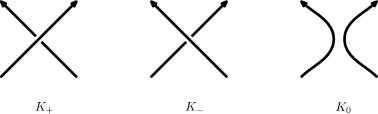
Figure 16. The skein triple $K_{+},\,K_{-}$ and $K_{0}.$

Lemma 7.12.

If $K$ is an almost classical knot, then $\Delta_{K}(-1)$ is odd.

Proof.

The skein formula of Theorem 7.11 shows that $\Delta_{K}(-1)\mod 2$ is independent under crossing changes. However, by changing the crossings of $K$, we can alter the diagram so that $K$ is ascending. But any ascending virtual knot diagram is necessarily welded trivial, and any welded trivial knot has trivial Alexander polynomial. Thus $\Delta_{K}(-1)\equiv 1\mod 2$ for any almost classical knot $K$, and this shows that $\Delta_{K}(-1)$ is odd. ∎

We now define the determinant of an almost classical knot or link. In case $K$ is an almost classical knot, Lemma 7.12 shows that $\det(K)$ is odd. In [33], Silver and Williams define the determinant of a long virtual knot using Alexander group systems.

Definition 7.13.

The determinant of an almost classical link $L$ is given by setting $\det(L)=|\Delta_{L}(-1)|$. Thus $\det(L)\in{\mathbb{Z}}$, and if $K$ an almost classical knot, then $\det(K)$ is odd.

Remark 7.14.

In the classical case, the determinant of a link $L$ satisfies $\det(L)=|H_{1}(X_{2})|,$ where $X_{2}$ denotes the double cover of $S^{3}$ branched along $L$, see Corollary 9.2 of [22]. (Note that $\det(L)=0$ means $H_{1}(X_{2})$ is infinite). For knots, $\det(K)$ is odd thus $H_{1}(X_{2})$ is always finite of odd order in that case.

There is a similar story for almost classical knots and links. Suppose $L$ is an almost classical link, which we view as a link in $Z=\Sigma\times I/\Sigma\times 1$, the space obtained by collapsing one component of the boundary of $\Sigma\times I$ to a point. If $F$ is a Seifert surface for $L$ in $\Sigma\times I$ and $V^{\pm}$ are the two Seifert matrices, then one can show that $V^{+}+V^{-}$ is a presentation matrix for $H_{1}(X_{2})$, where $X_{2}$ denotes the double cover of $Z$ branched along $L$. In particular, it follows that $\det(L)=|H_{1}(X_{2})|$, and Lemma 7.12 implies that $H_{1}(X_{2})$ is finite of odd order in the case $L=K$ is an almost classical knot.

In [28] the authors use the Alexander numbering of $K$ to prove that the first elementary ideal $\mathcal{E}_{1}$ is principal. Their proof extends to mod $p$ almost classical knots and links for $p\geq 2$ after making a change of rings which we now explain. Let $\zeta_{p}=e^{2\pi i/p}$ be a primitive $p$-th root of unity and consider the change of rings $\varphi\colon{\mathbb{Z}}[t^{\pm 1}]\to{\mathbb{Z}}[\zeta_{p}]$ given by setting $\varphi(t)=\zeta_{p}$.

Given a left ${\mathbb{Z}}[t^{\pm 1}]$-module $M$, we obtain the left ${\mathbb{Z}}[\zeta_{p}]$-module $M^{\prime}={\mathbb{Z}}[\zeta_{p}]\otimes_{{\mathbb{Z}}[t^{\pm 1}]}M$ where the right action of ${\mathbb{Z}}[t^{\pm 1}]$ on ${\mathbb{Z}}[\zeta_{p}]$ is given by $r\cdot a=r\varphi(a)$ for $a\in{\mathbb{Z}}[t^{\pm 1}]$ and $r\in{\mathbb{Z}}[\zeta_{p}]$. Note that if $M$ is finitely presented and $\left(a_{ij}\right)$ is a presentation matrix for $M$ then $\left(\varphi(a_{ij})\right)$ is a presentation matrix for $M^{\prime}$.

Thus, if $K$ is a mod $p$ almost classical knot, $p\geq 2$, then we define its Alexander “polynomial” to be an element $\Delta_{K}(\zeta_{p})\in{\mathbb{Z}}[\zeta_{p}]$ with $\mathcal{E}_{1}=(\Delta_{K}(\zeta_{p}))$ over ${\mathbb{Z}}[\zeta_{p}]$. As an invariant of mod $p$ almost classical knots, $\Delta_{K}(\zeta_{p})$ is well-defined up to units in ${\mathbb{Z}}[\zeta_{p}],$ and it is an invariant of the welded equivalence class of $K$.

The next proposition is the mod $p$ analogue of Corollary 7.3, and it follows by a straightforward generalization of the proof of Theorem 1.2 in [28].

Proposition 7.15.

Suppose $p\geq 2$ and that $K$ is a mod $p$ almost classical knot or link. Then the first elementary ideal $\mathcal{E}_{1}$ is principal over the ring ${\mathbb{Z}}[\zeta_{p}]$. ∎

8. Parity and projection

In this section, we introduce parity functions and the associated projection maps, and we explain their relationship with mod $p$ almost classical knots. Parity is a powerful tool with far-reaching implications, and we only give a brief account of it here. For more details, we refer the reader to Manuturov’s original article [24], his book [25], and the monograph [16].

Given a virtual knot diagram, a parity is a function that assigns to each classical crossing a value in $\{0,1\}$ such that the following axioms hold:

1. In a Reidemeister one move, the parity of the crossing is even.

2. In a Reidemeister two move, the parities of the two crossings are either both even or both odd.

3. In a Reidemeister three move, the parities of the three crossings are unchanged. Further, the three crossings can be all even, all odd, or one even and two odd. (I.e. we exclude the case that one crossing is odd and two are even.)

Note that this notion is referred to as “parity in the weak sense” by Manturov [26].

For example, recall the definition of the index $I(c_{i})$ of a chord in a Gauss diagram from Definition 1.1 and define

$$f(c_{i})=\begin{cases}0&\text{if $I(c_{i})\equiv 0$ mod $p$,}\\ 1&\text{if $I(c_{i})\not\equiv 0$ mod $p$.}\end{cases}$$

When $p=0$, then $f(c_{i})$ is called the Gaussian parity function. The proof that this is a parity follows from the properties of the index. Observe that $I(c_{i})=0$ for any chord involved in a Reidemeister one move, that $I(c_{i})=-I(c_{j})$ for any two chords involved in a Reidemeister two move, and that, for any three chords involved in a Reidemeister three move, $I(c_{i}),I(c_{j}),$ and $I(c_{k})$ are unchanged and satisfy $I(c_{i})+I(c_{j})=I(c_{k})$. These observations imply that the function $f$ defined above satisfies the parity axioms.

Here we remark that in general there are many parity functions that can be defined on Gauss diagrams, but the parity function $f$ described above is ideally suited to studying mod $p$ almost classical knots, as we now explain.

Given a virtual knot diagram $D$, we say that a chord $c$ is even if $f(c)=0$ and odd if $f(c)\neq 0$. We will define a map

$$P_{f}\colon\{\text{Gauss diagrams}\}\longrightarrow\{\text{Gauss diagrams}\}$$

called the Manturov projection map as its definition was inspired by [26] as follows. If $D$ has only even chords, then $P_{f}(D)=D.$ Otherwise, if it has odd chords, then let $P_{f}(D)$ be the Gauss diagram $D\smallsetminus\{c\mid f(c)=1\}$ obtained by removing the odd chords. Note that there can be even chords in $D$ that become odd in $P_{f}(D).$ In terms of the virtual knot diagram, one removes odd crossings by virtualizing them. Notice that a diagram $D$ admits a mod $p$ Alexander numbering if and only if $P_{f}(D)=D.$ Thus a virtual knot $K$ is mod $p$ almost classical precisely when it has a diagram that is fixed under $P_{f}.$

For example, Figure 17 shows two Gauss diagrams. The one on the left has six chords, exactly two of which are odd with respect to the Gaussian parity. Under projection, it is sent to the almost classical knot $4.99$ whose Gauss diagram appears on the right.

Figure 17. Manturov projection $P_{f}$ sends the diagram on the left to the one on the right.

The following lemma is crucial and implies that $P_{f}$ is well-defined as a map on virtual knots.

Lemma 8.1.

The Manturov projection map respects Reidemeister equivalence, i.e., if $D$ is Reidemeister equivalent to $D^{\prime}$, then $P_{f}(D)$ is Reidemeister equivalent to $P_{f}(D^{\prime})$.

Proof.

It is enough to prove the statement in the special case where $D$ and $D^{\prime}$ are related by just one Reidemeister move.

Assume first that $D$ and $D^{\prime}$ are related by a Reidemeister one move. By the parity axioms, the chord involved in the Reidemeister one move is even. Further, we see that this chord move does not intersect any of the other chords of the Gauss diagram. This means that $P_{f}(D)$ is identical to $P_{f}(D^{\prime})$ outside of the local neighbourhood of the Reidemeister move. Thus $P_{f}(D)$ is related to $P_{f}(D^{\prime})$ by a Reidemeister one move.

Now assume that $D$ and $D^{\prime}$ are related by a Reidemeister two move. Thus, two chords of opposite sign are added. Although the new chords may intersect other chords of the diagram, because they have opposite signs, they do not change the indices of any other chords. This means that $P_{f}(D)$ is identical to $P_{f}(D^{\prime})$ outside of the local neighbourhood of the Reidemeister two move.

The parity axioms imply that the two chords involved in the Reidemeister two move are either both even or both odd. If they are both even, then $P_{f}(D)$ is related to $P_{f}(D^{\prime})$ by a Reidemeister two move. If they are both odd, then we have $P_{f}(D)=P_{f}(D^{\prime})$.

Finally, suppose $D$ and $D^{\prime}$ are related by a Reidemeister three move. Reidemeister three moves do not change the indices of any the chords in the diagram. By the parity axioms, either all three chords are even, or all three are odd, or exactly two of them are odd. If all three chords are even, then $P_{f}(D)$ is related to $P_{f}(D^{\prime})$ by a Reidemeister three move. If all three chords are odd or if exactly two chords are odd, then we have $P_{f}(D)=P_{f}(D^{\prime}).$ ∎

The next result implies that the set of mod $p$ almost classical knots and links form a self-contained knot theory under the generalized Reidemeister moves. It is a consequence of Lemma 8.1 and repeated application of the projection $P_{f}$.

Proposition 8.2.

Let $D$ and $D^{\prime}$ be two Gauss diagrams that both admit mod $p$ Alexander numberings. If $D$ is Reidemeister equivalent to $D^{\prime}$, then they are related by a sequence of Reidemeister moves through Gauss diagrams that admit mod $p$ Alexander numberings.

For a virtual knot $K$ represented by a diagram $D$, we let $P_{f}(K)$ be the virtual knot represented by the diagram $P_{f}(D)$. Lemma 8.1 implies that this map is well-defined as a map of virtual knots. Notice further that $P_{f}(K)=K$ if and only if $K$ is a mod $p$ almost classical knot.

Since $P_{f}^{2}\neq P_{f},$ it is not idempotent and so $P_{f}$ is not a projection in the strict sense. However, for any given virtual knot $K$, there is an integer $n$ such that $P_{f}^{n+1}(K)=P_{f}^{n}(K).$ Thus, $P_{f}$ is eventually idempotent. In that case, it follows that $P_{f}^{n}(K)$ is mod $p$ almost classical, thus every virtual knot eventually projects to a mod $p$ almost classical knot under $P_{f}$. Thus, associated to every virtual knot $K$ is a canonical mod $p$ almost classical knot $K^{\prime}=P_{f}^{n}(K),$ and using this association we see that any invariant of mod $p$ almost classical knots can be lifted to give an invariant of virtual knots.

For example, one can extend Definition 7.6 to all virtual knots $K$ by defining $\Delta_{K}(t):=\Delta_{K^{\prime}}(t),$ where $K^{\prime}=P_{f}^{n}(K)$ is the image of $K$ under stable Manturov projection. (Here $f$ denotes the usual Gaussian parity, which implies that $K^{\prime}$ is almost classical for $n$ sufficiently large.)

Let $\mathcal{V}$ denote the set of all virtual knots and for $n\geq 0,$ define

$$\mathcal{V}^{p}_{n}=\{K\in\mathcal{V}\mid P_{f}^{n}(K)\text{ is a mod $p$ almost classical knot}\}.$$

This gives an ascending filtration

(8) $$\mathcal{V}^{p}_{0}\subset\mathcal{V}^{p}_{1}\subset\cdots\subset\mathcal{V}^{p}_{n-1}\subset\mathcal{V}^{p}_{n}\subset\cdots\mathcal{V},$$

on the set $\mathcal{V}$ of all virtual knots with the bottom $\mathcal{V}^{p}_{0}$ consisting of the mod $p$ almost classical knots. We say that $K\in\mathcal{V}$ lies in level $n$ if $K\in\mathcal{V}_{n}^{p}\smallsetminus\mathcal{V}^{p}_{n-1}$.

For example, let $p=0$ and consider the projections of the knot $K=6.3555$, whose Gauss diagram is on the left of Figure 18. It has two odd chords, and removing them gives the Gauss diagram for 4.9, in the middle of Figure 18. This knot also has two odd chords, and removing them gives the Gauss diagram on the right of Figure 18, which we note is 2.1, hence non-trivial. Since the next projection $P_{f}^{3}(K)$ is trivial, it follows that $K\in\mathcal{V}_{3}\smallsetminus\mathcal{V}_{2}$. Thus $K$ lies in level 3.

Figure 18. The Gauss diagrams of $K=6.3555$, $P_{f}(K)=4.9$, and $P_{f}^{2}(K)=2.1.$

Manturov’s projection map is especially useful for studying almost classical knots because it implies that any minimal crossing diagram for a mod $p$ almost classical knot is mod $p$ Alexander numberable. This observation is stated in the next theorem and is key to our tabulation of mod $p$ almost classical knots up to $6$ crossings in Section 9.

Theorem 8.3.

If $K$ is a mod $p$ almost classical knot, then any minimal crossing diagram for $K$ is mod $p$ Alexander numberable.

Proof.

Let $K$ be a mod $p$ almost classical knot and suppose that $D$ is a minimal diagram for $K$. Let $D^{\prime}$ be a Gauss diagram of $K$ that has a mod $p$ Alexander numbering. Since $D$ and $D^{\prime}$ both represent the same knot, they are Reidemeister equivalent. Since $D^{\prime}$ has an mod $p$ Alexander numbering, $P_{f}(D^{\prime})=D^{\prime}$. By Lemma 8.1, $P_{f}(D)$ is Reidemeister equivalent to $P_{f}(D^{\prime})=D^{\prime}$. Thus $P_{f}(D)$ is Reidemeister equivalent to $D$. Since $D$ is minimal, and since the projection map $P_{f}$ can only remove chords, it follows that $P_{f}(D)=D$. Thus all chords of $D$ are even, and this implies that $D$ also admits a mod $p$ Alexander numbering. ∎

For example, we apply this to Kishino’s knot in Figure 19 with $p=2$ to see that no diagram for this knot admits a mod 2 Alexander numbering. This resolves a question raised in Remark 3.11 of [8].

Figure 19. The minimal crossing diagram for Kishino’s knot is not mod $2$ Alexander numberable, thus no diagram of it is mod $2$ Alexander numberable.

9. Enumeration of almost classical knots

In [15], Green has classified virtual knots up to six crossings. Since the virtual knots in his tabulation all have minimal crossing diagrams, by Proposition 8.3, to check whether a given virtual knot is mod $p$ almost classical, it is enough to check which diagrams in Green’s table admit mod $p$ Alexander numberings. This is done by computer by computing the indices of all the chords in the Gauss diagram and seeing whether they are all equal to zero mod $p$. These calculations were performed using Matlab. For brevity, Table 1 includes only the numbers of mod $p$ almost classical knots for $p=0,2,3,4,5$, and we also give a complete enumeration of the almost classical knots up to six crossings, along with computations of their Alexander polynomials $\Delta_{K}(t)$ and their virtual genus $g(\Sigma_{K})$ in Table 2. Recall that $\Sigma_{K}$ is the Carter surface associated to $K$, and here we make use of Corollary 1 in [26], which states that if $K$ is a minimal crossing diagram, then its Carter surface $\Sigma_{K}$ has minimal genus. The proof is similar in spirit to the proof of Theorem 8.3, though in the place of the parity function $f$ above, Manturov’s argument uses homological parity.

Interestingly, every almost classical knot in Table 2 with trivial Alexander polynomial also has trivial knot group, and a case-by-case argument reveals that each one of them is in fact welded trivial.

Based on the low crossing examples, it is tempting to conjecture that almost classical knots $K$ have isomorphic upper and lower knot groups. We say that $K$ satisfies the twin group property if $G_{K}$ and $G_{K^{*}}$ are isomorphic. Here $K^{*}$ is the vertical mirror image of $K$, which is the knot obtained from $K$ by switching all the real crossings. In terms of Gauss diagrams, it is obtained by reversing all the chords and changing their signs.

Classical knots satisfy the twin group property, and this follows easily by interpreting the knot group $G_{K}$ as the fundamental group $\pi_{1}(S^{3}\smallsetminus\tau K)$ of the knot complement. Using the tabulation of almost classical knots, one can further check that the four-crossing and five-crossing almost classical knots also satisfy the twin group property. However, there are counterexamples among the six-crossing almost classical knots. The first is the almost classical knot $K=6.73053,$ which has

$$G_{K} = \langle a,b\mid a^{-1}b^{-1}a^{-1}bab\rangle$$

$$G_{K^{*}} = \langle a,b\mid a^{-1}b^{-1}a^{-1}bab,a^{3}b^{-3}aba^{-2}b^{2}a^{-1}b^{-1}\rangle.$$

Notice that the first relation for these groups is identical, and by counting representations into the symmetric group $S_{4}$ on four letters, one can show that $G_{K}\not\cong G_{K^{*}}$. There are several other almost classical knots with $G_{K}\not\cong G_{K^{*}}$, and they include the virtual knots $6.76479,\,6.78358,\,6.87188,\,6.89815$ and $6.90115$. In all cases, the groups $G_{K}$ and $G_{K^{*}}$ can be distinguished by counting representations into $S_{4}$ or $S_{5}.$

Crossing	virtual	mod $2$	mod $3$	mod $4$	mod $5$	almost	classical
number	knots	AC	AC	AC	AC	classical	knots
2	1	0	0	0	0	0	0
3	7	3	1	1	1	1	1
4	108	10	6	3	3	3	1
5	2448	104	21	17	11	11	2
6	90235	1557	192	81	71	61	5

Table 1. The numbers of mod $p$ almost classical knots up to $6$ crossings.

Knot $g$ Alexander polynomial ${3.6}$ 0 $t^{2}-t+1$ 4.99 1 $2t-1$ 4.105 1 $2t^{2}-2t+1$ ${4.108}$ 0 $t^{2}-3t+1$ 5.2012 2 $1$ 5.2025 2 $1$ 5.2080 1 $1$ 5.2133 2 $2t-1$ 5.2160 1 $t^{2}-t+1$ 5.2331 1 $t^{3}-t+1$ 5.2426 1 $(t^{2}-t+1)^{2}$ 5.2433 2 $t^{4}-2t^{3}+4t^{2}-3t+1$ ${5.2437}$ 0 $2t^{2}-3t+2$ 5.2439 1 $t^{3}-2t^{2}+3t-1$ ${5.2445}$ 0 $t^{4}-t^{3}+t^{2}-t+1$ 6.72507 2 $1$ 6.72557 2 $1$ 6.72692 2 $1$ 6.72695 1 $1$ 6.72938 2 $t^{2}-t+1$ 6.72944 1 $2t-1$ 6.72975 2 $1$ 6.73007 2 $1$ 6.73053 1 $t^{2}-t+1$ 6.73583 2 $1$ 6.75341 1 $2t-1$ 6.75348 2 $t-2$ 6.76479 2 $t^{2}-t+1$ 6.77833 2 $t^{2}-t+1$ 6.77844 2 $t^{2}-t+1$ 6.77905 2 $t^{2}-3t+1$ 6.77908 1 $2t^{2}-2t+1$ 6.77985 2 $t^{2}-t+1$ 6.78358 2 $t^{2}-3t+1$ 6.79342 1 $t^{2}-3t+1$ 6.85091 1 $t^{2}+t-1$ 6.85103 1 $t^{3}-t^{2}+2t-1$ 6.85613 2 $t^{2}-2t+2$ Knot $g$ Alexander polynomial 6.85774 2 $t^{3}-t^{2}+1$ 6.87188 1 $(2t-1)(t^{2}-t+1)$ 6.87262 2 $(t^{2}-t+1)^{2}$ 6.87269 1 $(2t-1)^{2}$ 6.87310 1 $t^{4}-t^{3}+2t^{2}-2t+1$ 6.87319 2 $3t^{2}-3t+1$ 6.87369 2 $t^{3}-2t^{2}+3t-1$ 6.87548 1 $t^{3}-2t^{2}-t+1$ 6.87846 1 $t^{3}-2t^{2}-t+1$ 6.87857 1 $t^{2}-4t+2$ 6.87859 1 $3t^{2}-3t+1$ 6.87875 1 $t^{3}+t^{2}-2t+1$ 6.89156 1 $2t^{3}-t^{2}-t+1$ 6.89187 0 $(t^{2}-t+1)^{2}$ 6.89198 0 $(t^{2}-t+1)^{2}$ 6.89623 1 $2t^{2}-2t+1$ 6.89812 1 $t^{3}-2t+2$ 6.89815 1 $2t-1$ 6.90099 2 $t^{4}-t^{2}+1$ 6.90109 1 $(2t^{2}-2t+1)(t^{2}-t+1)$ 6.90115 1 $(t^{2}-3t+1)(t^{2}-t+1)$ 6.90139 1 $(3t^{2}-3t+1)(t^{2}-t+1)$ 6.90146 2 $t^{4}-5t^{3}+9t^{2}-5t+1$ 6.90147 2 $t^{4}-3t^{3}+6t^{2}-5t+2$ 6.90150 1 $t^{4}-5t^{3}+6t^{2}-4t+1$ 6.90167 1 $t^{4}-2t^{3}+4t^{2}-4t+2$ 6.90172 0 $t^{4}-3t^{3}+5t^{2}-3t+1$ 6.90185 2 $3t^{4}-6t^{3}+6t^{2}-3t+1$ 6.90194 1 $t^{4}-4t^{3}+8t^{2}-5t+1$ 6.90195 1 $2t^{4}-3t^{3}+3t^{2}-2t+1$ 6.90209 0 $t^{4}-3t^{3}+3t^{2}-3t+1$ 6.90214 1 $3t^{2}-4t+2$ 6.90217 1 $t^{3}-4t^{2}+3t-1$ 6.90219 1 $2t^{3}-3t^{2}+3t-1$ 6.90227 0 $(t-2)(2t-1)$ 6.90228 1 $4t^{2}-6t+3$ 6.90232 1 $2t^{3}-6t^{2}+4t-1$ 6.90235 2 $t^{4}-3t^{3}+5t^{2}-3t+1$

Table 2. The virtual genus $g=g(\Sigma_{K})$ and Alexander polynomial for almost classical knots with up to six crossings.

Concluding remarks. In closing, we remark that one can develop similar results for long virtual knots. For instance, given a long virtual knot, there are natural definitions for the virtual knot group $\operatorname{\it VG}_{K}$, the reduced virtual knot group $\operatorname{\it\hbox{ \kern 0.09995pt\vbox{\hrule height=0.5pt\kern 1.07639pt\hbox{\kern-1.99997pt$G$\kern-0.50003pt}}\kern-0.29999pt}}_{K}$, the extended group $\operatorname{\it EG}_{K}$, and the quandle groups $\operatorname{\it QG}_{K}$, and one can prove analogues to Theorems 3.1 and 3.3 for long virtual knots.

The corresponding theory of Alexander invariants is actually much simpler because the first elementary ideals associated to each of these groups are in general principal for long virtual knots. Particularly nice is the case of almost classical long knots as many of the invariants of classical knots extend in the most natural way. This follows by viewing virtual knots as knots in thickened surfaces and interpreting long virtual knots as knots in thickened surfaces with a choice of basepoint. Drilling a small vertical hole through the thickened surface $\Sigma\times I$ at the basepoint results in 3-manifold $M$ with $\partial M$ connected. In particular, $M$ is a quasi-cylinder with $H_{2}(M)=0,$ and this is precisely the condition required to extend classical knot invariants to quasi-cylinders in the paper [10] by Cimasoni and Turaev. For instance, by appealing to the results in [10], one can define a Conway normalized Alexander polynomial, knot signatures, etc. We plan to address these questions in future work, where we hope to develop the corresponding results on virtual knot groups and almost classicality for long virtual knots.

Acknowledgements

We extend our thanks to Dror Bar-Natan, Ester Dalvit, Emily Dies, Jim Hoste and Vassily Manturov for their valuable input. H. Boden and A. Nicas were supported by grants from the Natural Sciences and Engineering Research Council of Canada, and R. Gaudreau was supported by a Postgraduate Scholarship from the Natural Sciences and Engineering Research Council of Canada.

${3.6=3_{1}}$                4.99                4.105

${4.108=4_{1}}$             5.2012             5.2025

5.2080                5.2133                5.2160

5.2331                5.2426                5.2433

$5.2437=5_{2}$                5.2439    $5.2445=5_{1}$

6.72507              6.72557              6.72692

6.72695              6.72938              6.72944

6.72975              6.73007              6.73053

6.73583              6.75341              6.75348

6.76479              6.77833              6.77844

6.77905              6.77908              6.77985

6.78358              6.79342              6.85091

6.85103              6.85613              6.85774

6.87188              6.87262              6.87269

6.87310              6.87319              6.87369

6.87548              6.87846              6.87857

6.87859              6.87875              6.89156

$\stackrel{{\scriptstyle\hbox{$6.89187\quad$}}}{{\hbox{$=3_{1}\#3_{1}$}}}$    $\stackrel{{\scriptstyle\hbox{$6.89198\quad$}}}{{\hbox{$=3_{1}\#3_{1}^{*}$}}}$           6.89623

6.89812              6.89815              6.90099

6.90109              6.90115              6.90139

6.90146              6.90147              6.90150

6.90167           $6.90172=6_{3}$           6.90185

6.90194           6.90195           $6.90209=6_{2}$

6.90214           6.90217           6.90219

$6.90227=6_{1}$           6.90228

6.90232           6.90235

Figure 20. 76 Gauss diagrams of almost classical knots with up to six crossings, including the nine classical knots $3_{1},4_{1},5_{1},5_{2},6_{1},6_{2},6_{3},3_{1}\#3_{1},$ and $3_{1}\#3_{1}^{*}$ as indicated.

References

- [1] J. W. Alexander. Topological invariants of knots and links. Trans. Amer. Math. Soc., 30(2):275–306, 1928. MR 1501429
- [2] V. G. Bardakov and P. Bellingeri. Groups of virtual and welded links. J. Knot Theory Ramifications, 23(3):1450014 (23 pages), 2014. MR 3200494
- [3] H. U. Boden, E. Dies, A. I. Gaudreau, A. Gerlings, E. Harper, and A. J. Nicas. Alexander invariants of virtual knots, J. Knot Theory Ramifications, 24(3): 1550009 (62 pages), 2015.
- [4] G. Cairns and D. M. Elton. The planarity problem for signed Gauss words. J. Knot Theory Ramifications, 2(4):359–367, 1993. MR 1247573 (95a:57032)
- [5] G. Cairns and D. M. Elton. The planarity problem. II. J. Knot Theory Ramifications, 5(2):137–144, 1996. MR 1395774 (97i:57023)
- [6] J. S. Carter. Classifying immersed curves. Proc. Amer. Math. Soc., 111(1):281–287, 1991. MR 1043406 (91d:57002)
- [7] J. S. Carter, S. Kamada, and M. Saito. Stable equivalence of knots on surfaces and virtual knot cobordisms. J. Knot Theory Ramifications, 11(3):311–322, 2002. Knots 2000 Korea, Vol. 1 (Yongpyong). MR 1905687 (2003f:57011)
- [8] J. S. Carter, D. S. Silver, S. G. Williams, M. Elhamdadi, and M. Saito. Virtual knot invariants from group biquandles and their cocycles. J. Knot Theory Ramifications, 18(7):957–972, 2009. MR 2549477 (2010i:57026)
- [9] Z. Cheng and H. Gao. A polynomial invariant of virtual links. J. Knot Theory Ramifications, 22(12):1341002, 33, 2013. MR 3149308
- [10] D. Cimasoni and V. Turaev. A generalization of several classical invariants of links. Osaka J. Math., 44(3):531–561, 2007. MR 2360939 (2008k:57023)
- [11] P. Cromwell. Knots and links, Cambridge University Press, Cambridge, 2004. MR 2107964 (2005k:57011)
- [12] R. H. Fox. Free differential calculus. I. Derivation in the free group ring. Ann. of Math. (2), 57:547–560, 1953. MR 0053938 (14,843d)
- [13] C. A. Giller. A family of links and the Conway calculus. Trans. Amer. Math. Soc., 270:75–109, 1982. MR 0642331 (83j:57001)
- [14] M. Goussarov, M. Polyak, and O. Viro. Finite-type invariants of classical and virtual knots. Topology 39(5):1045–1068, 2000. MR 1763963 (2001i:57017)
- [15] J. Green. A table of virtual knots, 2004. Information available online at www.math.toronto.edu/drorbn/Students/GreenJ/.
- [16] D. P. Ilyutko, V. O. Manturov, and I. Nikonov. Parity in knot theory and graph links. Sovrem. Mat. Fundam. Napravl., 41:3–163, 2011. MR 3011999
- [17] N. Kamada and S. Kamada. Abstract link diagrams and virtual knots. J. Knot Theory Ramifications, 9(1):93–106, 2000. MR 1749502 (2001h:57007)
- [18] L. H. Kauffman. Virtual knot theory. European J. Combin., 20(7):663–690, 1999. MR 1721925 (2000i:57011)
- [19] L. H. Kauffman and D. Radford. Bi-oriented quantum algebras, and a generalized Alexander polynomial for virtual links. In Diagrammatic morphisms and applications (San Francisco, CA, 2000), volume 318 of Contemp. Math., pages 113–140. Amer. Math. Soc., Providence, RI, 2003. MR 1973514 (2004c:57013)
- [20] S. Kim. Virtual knot groups and their peripheral structure. J. Knot Theory Ramifications, 9(6):797–812, 2000. MR 1775387 (2001j:57010)
- [21] G. Kuperberg. What is a virtual link? Algebr. Geom. Topol., 3:587–591 (electronic), 2003. MR 1997331 (2004f:57012)
- [22] W. B. Raymond Lickorish. An introduction to knot theory, volume 175 of Graduate Texts in Mathematics. Springer-Verlag, New York, 1997. MR 1472978 (98f:57015)
- [23] V. O. Manturov. On invariants of virtual links. Acta Appl. Math., 72(3):295–309, 2002. MR 1916950 (2004d:57010)
- [24] V. O. Manturov. Parity in knot theory. Mat. Sb., 201(5):65–110, 2011. MR 2681114 (2011g:57009)
- [25] V. O. Manturov and D. P. Ilyutko. Virtual knots, Series on Knots and Everything, vol. 51, World Scientific Publishing Co. Pte. Ltd., Hackensack, NJ, 2013, The state of the art, Translated from the 2010 Russian original, With a preface by Louis H. Kauffman. MR 2986036
- [26] V. O. Manturov. Parity and projection from virtual knots to classical knots. J. Knot Theory Ramifications, 22(9):1350044, 20, 2013. MR 3105303
- [27] V. O. Manturov and D. P. Ilyutko, Virtual knots, Series on Knots and Everything, vol. 51, World Scientific Publishing Co. Pte. Ltd., Hackensack, NJ, 2013, The state of the art, Translated from the 2010 Russian original, With a preface by Louis H. Kauffman. MR 2986036
- [28] T. Nakamura, Y. Nakanishi, S. Satoh, and Y. Tomiyama. Twin groups of virtual 2-bridge knots and almost classical knots. J. Knot Theory Ramifications, 21(10):1250095, 18, 2012. MR 2949227
- [29] Andrew Ranicki. High-dimensional knot theory. Springer Monographs in Mathematics. Springer-Verlag, New York, 1998. Algebraic surgery in codimension 2, With an appendix by Elmar Winkelnkemper. MR 1713074 (2000i:57044)
- [30] J. Sawollek. On Alexander-Conway polynomials for virtual knots and links, 1999 preprint, arxiv.org/pdf/math/9912173.pdf
- [31] D. S. Silver and S. G. Williams. Alexander groups and virtual links. J. Knot Theory Ramifications, 10(1):151–160, 2001. MR 1822148 (2002b:57014)
- [32] D. S. Silver and S. G. Williams. Polynomial invariants of virtual links. J. Knot Theory Ramifications, 12(7):987–1000, 2003. MR 2017967 (2004i:57015)
- [33] D. S. Silver and S. G. Williams. Alexander groups of long virtual knots. J. Knot Theory Ramifications, 15(1):43–52, 206. MR 2204496 (2006j:57023)
- [34] D. S. Silver and S. G. Williams. Crowell’s derived group and twisted polynomials. J. Knot Theory Ramifications, 15(8):1079–1094, 2006. MR 2275098 (2008i:57011)