Search for Early Gamma-ray Production in Supernovae Located in a Dense Circumstellar Medium with the Fermi LAT

Abstract

Supernovae (SNe) exploding in a dense circumstellar medium (CSM) are hypothesized to accelerate cosmic rays in collisionless shocks and emit GeV $\gamma$ rays and TeV neutrinos on a time scale of several months. We perform the first systematic search for $\gamma$-ray emission in Fermi LAT data in the energy range from $100\,$MeV to $300\,$GeV from the ensemble of 147 SNe Type IIn exploding in dense CSM. We search for a $\gamma$-ray excess at each SNe location in a one year time window. In order to enhance a possible weak signal, we simultaneously study the closest and optically brightest sources of our sample in a joint-likelihood analysis in three different time windows (1 year, 6 months and 3 months). For the most promising source of the sample, SN 2010jl (PTF10aaxf), we repeat the analysis with an extended time window lasting 4.5 years. We do not find a significant excess in $\gamma$ rays for any individual source nor for the combined sources and provide model-independent flux upper limits for both cases. In addition, we derive limits on the $\gamma$-ray luminosity and the ratio of $\gamma$-ray-to-optical luminosity ratio as a function of the index of the proton injection spectrum assuming a generic $\gamma$-ray production model. Furthermore, we present detailed flux predictions based on multi-wavelength observations and the corresponding flux upper limit at $95\%$ confidence level (CL) for the source SN 2010jl (PTF10aaxf).

Keywords. Methods: data analysis; cosmic rays, gamma rays, supernova

1 Introduction

The Large Area Telescope (LAT) on-board the Fermi Gamma-ray Space Telescope mission unanticipatedly detected $\gamma$-ray emission from five Galactic novae (Abdo et al., 2010; Hill et al., 2013; Hays et al., 2013; Cheung et al., 2013). The origin of the $\gamma$-ray emission is still unclear. Shocks produced by expansion of the nova shell into the wind provided by the companion star or internal shocks within the ejecta might be responsible for acceleration of particles to relativistic energies and ensuing high-energy $\gamma$-ray emission. A similar mechanism but with much larger energy output is hypothesized to produce $\gamma$ rays in supernovae (SNe) yielding potentially detectable $\gamma$-ray emission even from extragalactic sources. Murase et al. (2011, 2014) and Katz et al. (2011) showed that if the SN progenitor is surrounded by an optically thick circumstellar medium (CSM), then a collisionless shock is necessarily formed after the shock breakout. The collisionless shock may accelerate protons and electrons to high energies, which emit photons from the radio-submillimeter through GeV energies and TeV neutrinos. Such conditions appear in shocks propagating through dense circumstellar matter (e.g., wind). Recently several candidates for such SNe powered by interactions with a dense CSM were found (e.g., Ofek et al., 2007, 2014a; Smith et al., 2009; Zhang et al., 2012) and some superluminous supernovae were suggested to be powered by interactions (e.g., Quimby et al., 2011; Chevalier & Irwin, 2011). Such interaction-powered supernovae may also be Pevatrons, implying their importance for the origin of the knee structure in the cosmic-ray spectrum (Murase et al., 2014; Sveshnikova, 2003). Both $\gamma$ rays and neutrinos originate from pp and p$\gamma$ interactions producing pions, which in the neutral case decay to $\gamma$ rays and in the charged case produce neutrinos in the decay chain. Thus, the initial neutrino and $\gamma$-ray spectra have the same shape. Contrary to neutrinos, $\gamma$ rays might be affected by absorption in the CSM and/or two-photon annihilation with low-energy photons produced at the forward shock (Murase et al., 2011). However, arguments made in Murase et al. (2014) suggest that GeV $\gamma$ rays can escape the system without severe attenuation, if the shock velocity is in the right range, especially late after the shock breakout.

Motivated by the fact that the LAT has detected $\gamma$-ray emission from novae, we are presenting the first systematic search for $\gamma$-ray emission from Type IIn SNe in Fermi LAT data from $100\,$MeV to $300\,$GeV. Considering current theoretical uncertainties we are aiming for a model independent search. SNe positions and explosion times are given by optical surveys such as the Palomar Transient Factory (PTF – Law et al., 2009; Rau et al., 2009).

We present the sample of SNe used in the $\gamma$-ray data analysis in Section 2. Section 3 describes the Fermi LAT data analysis followed by an interpretation of our results in Section 4 and conclusions in Section 5.

2 SNe Sample

Type IIn and Type Ibn SNe are the best candidates to be interacting with a dense CSM. Their long-lasting bright optical light curves are believed to be powered by the interaction of the ejecta with massive CSM (Svirski et al., 2012). SNe of these types are often accompanied by precursor mass-ejection events (Ofek et al., 2014b). Here we mainly use the PTF SN sample along with publicly available Type IIn SNe discovered since the launch of Fermi in 2008. Appendix A lists all $147$ SNe of this sample that we consider in our $\gamma$-ray search, i.e., all sources with an estimated explosion time later than 2008 August 4 and before 2012 May 1 (this is one year before the end of the studied $\gamma$-ray data sample). The apparent $R$-band peak magnitude ($m$) as a function of the peak time is shown in Fig. 1. Note that throughout this paper we refer to $m$ as the peak magnitude; for sources where the peak magnitude is not determined we use the discovery magnitude instead. The subsample of bright ($m<16.5$) and/or nearby (with a redshift $z<0.015$) SNe used for the joint likelihood analysis is detailed in Table 2.

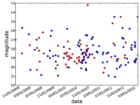
Figure 1: Apparent $R$-band peak (detection) magnitude as a function of the peak (detection) time shown in red (blue) for all 147 SNe in our sample. For some SNe the peak time and magnitude is not determined; in those cases we use the detection time and magnitude.

Name	RA (∘)⋆	Dec (∘)⋆	Date	z	m	TS (p-value)
SN2008gm	348.55	-2.78	2008-10-22$\dagger$	0.012	17.00$\ddagger$	3.2 (0.169)
SN2008ip	194.46	36.38	2008-12-31$\dagger$	0.015	15.70$\ddagger$	0.0 (0.572)
SN2009au	194.94	-29.60	2009-03-11$\dagger$	0.009	16.40$\ddagger$	0.0 (0.572)
PTF10ujc	353.63	22.35	2009-08-05	0.032	16.20	0.0 (0.572)
SN2009kr	78.01	-15.70	2009-11-06$\dagger$	0.006	16.00$\ddagger$	4.7 (0.104)
SN2010bt	192.08	-34.95	2010-04-17$\dagger$	0.016	15.80$\ddagger$	14.4 (0.0065)
PTF10aaxf	145.72	9.50	2010-11-18	0.011	13.20	7.1 (0.039)
SN2010jl
PTF10aaxi	94.13	-21.41	2010-11-23	0.010	18.00	0.0 (0.572)
SN2010jp
SN2011A	195.25	-14.53	2011-01-02$\dagger$	0.009	16.90$\ddagger$	0.0 (0.572)
PTF11iqb	8.52	-9.70	2011-08-06	0.013	15.20	0.3 (0.469)
SN2011fh	194.06	-29.50	2011-08-24$\dagger$	0.008	14.50$\ddagger$	1.9 (0.262)
PSNJ10081059+5150570	152.04	51.85	2011-10-29	0.004	14.50	0.0 (0.572)
SN2011ht
PTF11qnf	86.23	69.15	2011-11-01$\dagger$	0.014	19.80$\ddagger$	1.4 (0.320)
SN2011hw	336.56	34.22	2011-11-18$\dagger$	0.023	15.70$\ddagger$	0.0 (0.572)
SN2012ab	185.70	5.61	2012-01-31$\dagger$	0.018	15.80$\ddagger$	0.0 (0.572)
PSNJ18410706-4147374	280.28	-41.79	2012-04-25$\dagger$	0.019	14.50$\ddagger$	0.0 (0.572)
SN2012ca

• Epoch J2000.0

• Discovery date

• Discovery magnitude

List of nearby and/or bright SNe – with redshift $z<0.015$ and/or R-band magnitude $m<16.5$. The colums contain the name of the SN, its direction in equatorial coordinated (right ascension, RA, and declination, Dec), its peak date and peak R-band magnitude, its redshift, its test statistic (TS) and p-value. See Section 3.1 for details on the TS and p-value calculation. Note that if the peak date and magnitude are not available in the catalog, the discovery date and magnitude are quoted instead.

3 Fermi LAT $\gamma$-ray Data Analysis

The Fermi LAT is a pair-conversion telescope, sensitive to $\gamma$ rays with energies from $20\,$MeV to greater than $300\,$GeV (Atwood et al., 2009). It has a large field of view and has been scanning the entire sky every few hours for the last 6 years. Thus it is very well suited for searches for transient $\gamma$-ray signals on the timescale of months. Bright SN events may be detectable at distances $d<30$ Mpc (Murase et al., 2011) depending on the properties of the source. Margutti et al. (2014) searched for $\gamma$ rays from a single SN in the case of SN2009ip located at a distance of $24\,$Mpc. No $\gamma$-ray excess was identified in Fermi LAT data at the SN position; this is consistent with the picture of ejecta colliding with a compact and dense but low-mass shell of material. For a detection of a single source, closer and/or brighter SNe are needed (i.e., reached by larger dissipation and larger CSM masses). The properties of the ejecta and CSM can be estimated from multi-wavelength observations in a few cases (e.g., SN2009ip, Ofek et al., 2013), but are uncertain or not known in most cases.

In this analysis we use 57 months of Fermi LAT data recorded between 2008 August 4 and 2013 May 1 (Fermi Mission Elapsed Time 239557418–389092331 s), restricted to the Pass 7 Reprocessed Source class. We select the standard good time intervals (e.g., excluding time intervals when the field of view of the LAT intersected the Earth). The Pass 7 Reprocessed data benefit from an updated calibration that improves the energy measurement and event-direction reconstruction accuracy at energies above 1 GeV (Bregeon et al., 2013). To minimize the contamination from the $\gamma$ rays produced in the upper atmosphere, we select events with zenith angles $<100^{\circ}$. We perform a binned analysis (i.e., binned in space and energy) using the standard Fermi LAT ScienceTools package version v09r32p05 available from the Fermi Science Support Center (FSSC) using the P7REP_SOURCE_V15 instrument response functions. We analyze data in the energy range of 100 MeV to 300 GeV binned into 20 logarithmic energy intervals. For each source we select a $20^{\circ}\times 20^{\circ}$ region of interest (ROI) centered on the source localization binned in $0\fdg 2$ size pixels. The binning is applied in celestial coordinates and an Aitoff projection was used.

We use four different approaches in our analysis:

1. We perform a likelihood analysis to search for $\gamma$-ray excesses that are consistent with originating from a point source coincident with the position of each Type IIn SNe in our sample over a 1-year time scale. We assume that their $\gamma$-ray emission follows a power-law spectrum. This approach is sensitive to single bright sources.

2. In a model-independent approach (i.e., no prior assumption on the SN $\gamma$-ray spectral shape) we compute the likelihood in bins of energy (bin-by-bin likelihood). We use the bin-by-bin likelihood to evaluate $95$% CL flux upper limits in 20 energy bins for the 16 closest and optically brightest SNe in our sample.

3. In order to increase the sensitivity for a weak signal, we combine individual sources in a joint likelihood analysis using the composite likelihood tool, Composite2, of the Fermi  Science Tools.

4. We repeat the joint likelihood analysis using the composite likelihood tool, but limit the sample to those Type IIn SNe that exhibit additional indications of strong interactions with their CSM. Not all Type IIn SNe might be surrounded by a massive CSM. This clean sample of SNe with confirmed massive CSM might produce a strong $\gamma$-ray signal and should provide an enhanced signal-to-background ratio.

Accurate SN positions are given by optical localizations. Theoretical predictions of the duration of the $\gamma$-ray emission are uncertain and motivate a search in several time windows. We test three different time windows: $\Delta T=1$ year, 6 months and 3 months. The optical light curve is produced by the interaction of the SN ejecta with the dense CSM and is thus correlated with the expected $\gamma$-ray emission. Most of the $\gamma$-ray emission is expected during the interactions after the shock breakout. The optical light curve peak is reached around the end of the breakout (see e.g., Ofek et al., 2010). We collected the SN properties from the PTF sample, Astronomer’s Telegrams (ATels) and Central Bureau for Astronomical Telegrams (CBETs). Most PTF sources are unpublished and the other events were drawn from ATEL and CBET. Full details and final analysis of the PTF SN IIn sample will be provided in a forthcoming publication. In some cases the known SN properties include the optical flux peak time while in other cases this information is missing and only the optical detection time is available. To account for the uncertainty in the determination of the peak time and to make sure no early $\gamma$-ray emission is missed, we start the time window $30$ days before the peak time (or the detection time in case the peak time is not provided). In the case of the three novae, the reported $\gamma$-ray light curves (see Fig. 1 in Hill et al., 2013) have very similar durations justifying a similar time window for all sources. However, the duration of the novae detected by Fermi were $\sim 20$ days, while SN IIn typically last longer, $\mathcal{O}$(100 days - 1 year).

3.1 Source Specific Analysis

We analyze the $20^{\circ}\times 20^{\circ}$ ROI around each source in our SN sample in a 1-year time window in a binned likelihood analysis. We construct a model whose free parameters are fitted to the data in the ROI. This model includes a point-like source at the SN position; its $\gamma$-ray spectrum is represented as a power-law function with both index and normalization free to vary. In addition we have to model the point sources in the ROI and the diffuse $\gamma$-ray emission. We consider all the 2FGL sources (Nolan et al., 2012) included within a larger region of radius, $R=20^{\circ}$, to allow for the breadth of the LAT point-spread function that may cause a significant signal from sources outside the ROI to leak into it. The positions and spectral parameters of all 2FGL sources within $15^{\circ}<R<20^{\circ}$ from the center of the ROI are fixed to the values reported in the 2FGL catalog; those are on average 21 sources. For the sources within $5^{\circ}<R<15^{\circ}$ with $>15\sigma$ detection significance in 2FGL only the flux normalization is let free to vary and all the other parameters are fixed to the values reported in the 2FGL catalog. The parameters for all the other sources within $5^{\circ}<R<15^{\circ}$ are fixed to the 2FGL catalog values. Finally, for sources within $R<5^{\circ}$ all parameters (index and normalization in case of a power-law spectrum, index, cutoff and normalization in case of a power-law with exponential cutoff and normalization, spectral slope and curvature in case of a log-parabola source spectrum) are free to vary if the source significance exceeds $4\,\sigma$, otherwise all source parameters are fixed. On average 3 sources per ROI have all parameters free, while 6 sources have a free normalization and 18 sources are fixed to the 2FGL values.

We determine the best values for all the free parameters fitting our source model together with a template for the isotropic and Galactic interstellar emission to the LAT data with a binned likelihood approach as described in Abdo et al. (2009). To quantify the significance of a potential excess above the background, we employ the likelihood-ratio test  (Neyman & Pearson, 1928). We form a test statistic

$$TS=-2\Delta\log{\mathcal{L}}=-2(\log{\mathcal{L}_{0}}-\log{\mathcal{L}}),$$ (1)

where $\mathcal{L}_{0}$ is the likelihood evaluated at the best-fit parameters under a background-only, null hypothesis, i.e. a model that does not include a point source at the SN position, and $\mathcal{L}$ the likelihood evaluated at the best-fit model parameters when including a candidate point source at the SN position.

The distribution of the TS values obtained for all the SNs using a 1 year time window is displayed in Fig. 2 (left), compared to the TS distribution obtained from performing a similar analysis at random positions in the sky. We require the random ROI centers to be separated by at least $3.5^{\circ}$ and to lie outside of the Galactic plane, i.e. $|b|>10^{\circ}$. The analysis in the Galactic plane region is complicated by the intense Galactic diffuse emission and none of the SNe in our sample is located close to the plane. Those requirements limit the number of independent ROIs; we use 1140 ROIs in our analysis. The distribution of SN-position TS values is similar to the distribution of random-position TS values (see Fig. 2 left). The highest TS value found among the SN positions is 14.4, which corresponds to a p-value of $0.0065$ (obtained from the random position analysis), which is below $3\,\sigma$ for a single trial (see Fig. 2 right). Given the number of SNe in our sample a trials factor needs to be applied, which increases the p-value to $0.6$.

Optically bright SNe are expected to produce a brighter $\gamma$-ray signal than optically dim ones and nearby SNe are expected to be brighter than sources at large distance. However, we do not find an obvious correlation of TS value with redshift or magnitude (see left and right panels of Fig. 3, respectively), indicating that the $\gamma$-ray signals of individual SNe, if present, are weak.

Three of 147 SNe have a 2FGL source in their close vicinity with an angular distance of less than $0.4^{\circ}$. In each case the nearest 2FGL source is associated with an active galactic nucleus through multi-wavelength data. Since the spectral parameters of the nearby source are left free to vary in the fit, a possible SNe flux could have been absorbed by the background source. Those sources are PTF10weh, LSQ12by and SN 2012bq, which are optically dim and distant sources and thus not part of the subsample of nearby and/or bright SNe.

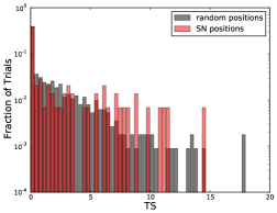
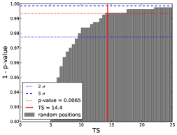
Figure 2: Left: Distribution of TS values for a test source modeled by a power-law energy spectrum located at a SN position (red), compared to TS for a similar test source located at a random position (grey). Right: Cumulative distribution of random-position TS values. The blue dashed (dotted) line indicates a Gaussian equivalent one-sided $3\,\sigma$ ($2\,\sigma$) probability of finding a larger TS than the TS indicated by the intersection of the blue line with the grey distribution. The red solid line shows the largest TS found in the source-specific analysis, which has a p-value of $0.0065$ (red dotted line) and thus lies below $3\,\sigma$. Considering the trials factor, the p-value increases to $0.6$.

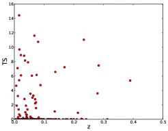
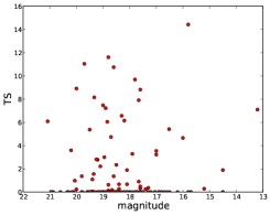
Figure 3: TS of a test source located at the SN position as function of redshift (left) and as function of magnitude (right). Note that the largest TS value was $14.4$ (corresponding to a p-value of $0.009$), which does not exceed the detection threshold of $5\,\sigma$.

3.2 Model independent analysis of nearby and/or bright SNe

The $\gamma$-ray spectral shape resulting from particle acceleration in the interaction of SN ejecta with a dense CSM is not known a priori. It is determined by the initial proton spectrum and could be altered by absorption of the $\gamma$ rays in the surrounding medium. Therefore, we study the closest and/or optically brightest sources, which are the most promising sources in terms of expected $\gamma$-ray emission, in an approach independent of a SN spectral model assumption. The sources chosen for this analysis have to fulfill the criteria of $z<0.015$ or $m<16.5$, and are listed in Table 2. We fix the spectral parameters of the background sources and the diffuse templates to their global values obtained from the source-by-source analysis over the entire energy range described in Section 3.1 (without including the SN itself). Following the procedure described in Ackermann et al. (2014) we calculate the likelihood in each of the 20 energy bins after inserting a test source at the SN position at various flux normalization values:

$$\mathcal{L}(\{\bm{\mu}_{j}\},\bm{\hat{\theta}}|\mathcal{D})=\prod_{j}\mathcal{L}_{j}(\bm{\mu}_{j},\bm{\hat{\theta}}|\mathcal{D}_{j}),$$ (2)

where $\mathcal{D}_{j}$ is the photon data, $\mathcal{L}_{j}$ the Poisson likelihood and $\{\bm{\mu}_{j}\}$ a set of independent signal parameters in energy bin $j$. The symbol $\bm{\theta}$ represents the nuisance parameter (i.e., free parameters of background sources and diffuse templates) and $\bm{\hat{\theta}}$ indicates that they have been fixed to their global values. The bin-by-bin likelihood allows us to find the upper limits at $95\%$ CL, defined as the value of the energy flux, where the log-likelihood decreases by $2.71/2$ from its maximum (the “delta-log-likelihood technique” – Bartlett, 1953; Rolke et al., 2005). An example is shown in Fig. 4 for SN 2010jl (PTF10aaxf – Ofek et al., 2014a; Fransson et al., 2014; Zhang et al., 2012), while similar plots for all nearby sources can be found in Appendix B. Any SN model predicting a certain $\gamma$-ray spectrum can be tested using those results (see Ackermann et al., 2014, for more details on the bin-by-bin likelihood) by recreating a global likelihood by tying together the signal parameters over the energy bins:

$$\mathcal{L}({\bm{\mu}},\bm{\hat{\theta}}|\mathcal{D})=\prod_{j}\mathcal{L}_{j}({\bm{\mu}_{j}(\bm{\mu})},\bm{\hat{\theta}}|\mathcal{D}_{j}),$$ (3)

with ${\bm{\mu}}$ denoting the global signal parameters.

For the most promising source of our sample, SN 2010jl, we repeat the analysis for an extended time window ending in May 2015, i.e., spanning 4.5 years. This is motivated by the fact that in some cases SN Type IIn emission lasts for 3-5 years after the explosion (Cooke et al., 2009).

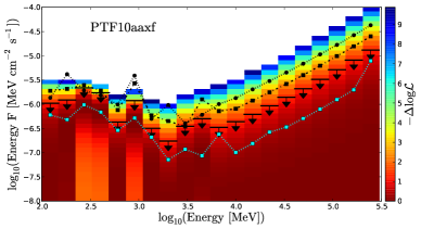
Figure 4: Histogram of the bin-by-bin LAT likelihood function used to test for a putative $\gamma$-ray source at the position of supernova SN 2010jl (PTF10aaxf). The bin-by-bin likelihood is calculated by scanning the integrated energy flux of the SN within each energy bin (equivalent to scanning in the spectral normalization of the source). When performing this scan, the flux normalizations of the background sources are fixed to their optimal values as derived from a maximum likelihood fit over the full energy range. Within each bin, the color scale denotes the variation of the logarithm of the likelihood with respect to the best-fit value of the SN flux using a 1 year time window. Upper limits on the integrated energy flux are set at 95% CL within each bin using the delta-log-likelihood technique and are largely independent of the SN spectrum. The black arrows indicate the 95% CL flux upper limits for $\Delta T=1$ yr, where the shown log-likelihood decreases by 2.71/2 from its maximum. For completeness we overlay the 95% CL upper limits for $~{}\Delta T=6$ months and $\Delta T=3$ represented by dotted-dashed and dotted lines respectively. For the particular case of SN 2010jl we repeated the analysis for an extended time window spanning 4.5 years. The results are overlaid as cyan dotted line.

3.3 Joint Likelihood Analysis

For greater sensitivity to a weak $\gamma$-ray signal from interaction-powered SNe, we combine the 16 closest and/or brightest sources in a joint likelihood analysis. To be independent from any spectral shape assumption we perform the analysis in energy bins (see Section 3.2 for details of the bin-by-bin likelihood analysis). In each energy bin we tie the SN flux normalization for all 16 SNe together resulting in one free parameter per energy bin. The likelihood values for the individual sources, $i$, are multiplied to form the joint likelihood:

$$\mathcal{L}(\bm{\mu},\{\bm{\hat{\theta}}_{i}\}|\mathcal{D})=\prod_{i}\mathcal{L}_{i}(\bm{\mu},\bm{\hat{\theta}}_{i}|\mathcal{D}_{i}).$$ (4)

However, we have to make some assumption about a common scaling factor of the $\gamma$-ray flux in order to tie the SNe flux normalizations together (i.e., we want to give a larger weight to SNe with greater expected $\gamma$-ray fluxes in the joint likelihood). We use two different approaches: first, we assume that all SNe have the same intrinsic $\gamma$-ray luminosity; therefore, the observed $\gamma$-ray flux for each SN scales with a factor inversely proportional to the square of the luminosity-distance $d$. The redshift is measured for each SNe and since we only consider nearby SNe we use a simple linear approximation for the relation between redshift and distance: $d=z\times c/H$, with $H=67.8$ km s^-1 Mpc^-1 (Ade et al., 2014). We do not apply a redshift-dependent energy rescaling for SNe at different redshifts, since the energy shift is negligible at the small redshifts (i.e., $z<0.015$) considered in this analysis. We weight the flux normalization in each energy bin of each source with $w_{d}=(10\,\textrm{Mpc}/d)^{2}$. We then tie those weighted normalizations together. The exact value of $H$ does not influence our results since the combined normalization of all sources is free in the fit of the model to the data in each energy bin. Note that only the SN flux normalization is free while the background source parameters as well as the diffuse template parameters are fixed to their global values obtained from a fit to the entire energy range.

Alternatively, we assume that the $\gamma$-ray flux is correlated with the optical flux, i.e. we use a weight proportional to the optical flux or $10^{-0.4m}$. We chose the weight to be:

$$w_{m}=10^{-0.4(m-C)}=10^{-0.4m+5.2},$$ (5)

where $m$ is the apparent $R$-band magnitude provided by the SN catalog and $C=13$ is a normalization constant. Again, the exact choice of $C$ does not influence our results since the combined normalization of all sources is free in the fit. We chose to neglect a correction for Galactic dust extinction, which is at most $0.28$ mag and thus smaller than the uncertainty in the peak magnitude determination.

We perform the joint likelihood analysis for three time windows: 1 year, 6 months, 3 months since the $R$-band maximum light. Fig. 5 shows the likelihood profiles of the combined $\gamma$-ray flux. Table 1 summarizes the results from the combined likelihood analysis and shows the sum of TS over all energy bins. No significant improvement in the likelihood by including the SNe in the fit could be found in the joint likelihood analysis. The largest TS value of $8.8$ is found in case of assuming the $\gamma$-ray flux scales with the optical flux for the 1-year time windows. According to Wilks’ theorem, TS is distributed approximately as $\chi^{2}$ with the degrees of freedom equal to the number of parameters characterizing the additional source. Taking into account the number of free parameters (20, one for each energy bin) the probability that this is a statistical fluctuation is $98.5\%$. This significance would be further decreased by taking into account trials factors for the two different weighting schemes and 3 different time windows.

However, if we assume a spectral model for the SN flux, we can greatly reduce the number of free parameters. For illustration we fit a power-law spectral shape to the bin-by-bin likelihood following Equation 3. The index and normalization of the power-law function are left free to vary in the fit. The resulting TS values and corresponding p-values (not including trials factors) are summarized in Table 1; none of them are significant. A more physical spectral model is fitted to the bin-by-bin likelihood in Section 4.

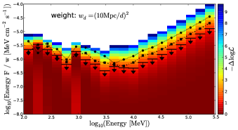
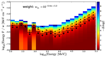
Figure 5: Similar to Fig. 4, but for the composite likelihood instead of the single-source likelihood. Left: Composite likelihood profile for each energy bin weighting each source with $(10$ Mpc$/d)^{2}$. Right: Composite likelihood profile for each energy bin weighting each source with $10^{-0.4m+5.2}$. The black arrows indicate the 95% upper limits for $\Delta T=1$ yr, while the dotted-dashed and dotted lines represent the 95% upper limits for $~{}\Delta T=6$ months and $\Delta T=3$ months, respectively.

Weighting	TS			TSPL (p-value)
	1 yr	6 months	3 months	1 yr	6 months	3 months
$(\rm{10\,Mpc}/d)^{2}$	2.2	2.1	2.4	0.0 (1.0)	0.0 (1.0)	0.0 (1.0)
$10^{-0.4m+5.2}$	11.7	7.8	9.0	2.9 (0.23)	1.6 (0.45)	0.0 (1.0)

Table 1: Sum over bin-by-bin TS values obtained from the joint likelihood analysis. TS_PL is the TS obtained by assuming a power-law spectral shape.

3.4 Joint Likelihood Analysis of SN Subsample with Confirmed Massive CSM

We select a subsample of 16 SNe from the Type IIn SNe catalog for which we have additional evidence through multi-wavelength observations for the existence of a massive CSM. We select SNe that show Balmer emission lines and continuum in both early and late times. The SNe in this sample are: PTF12csy, PTF11oxu, PTF11mhr, PTF11fzz, PTF11fuu, PTF10aaxf, PTF10ptz, PTF10scc, PTF10jop, PTF10fei, PTF10qaf, PTF10tel, PTF10tyd, PTF10gvf, PTF10cwl, PTF09drs. We repeat the joint likelihood analysis described above for this subset with the optical flux weighting scheme for three time windows (1 year, 6 months and 3 months). The results are displayed in Fig. 6. The TS values of the composite fit are 11.3, 17.5 and 10.3 for the time windows of 1 year, 6 months, and 3 months, respectively. Taking into account the 20 free parameters, the chance probability for a TS of 17.5 is $62\%$.

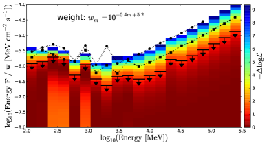
Figure 6: Joint likelihood analysis of the SN subsample with confirmed massive CSM: Joint likelihood profile for each energy bin weighting each source with $10^{-0.4m+5.2}$. The black arrows indicate the 95% upper limits for $\Delta T=1$ year, while the dotted-dashed and dotted lines represent the 95% upper limits for $~{}\Delta T=6$ months and $\Delta T=3$ months, respectively.

4 Interpretation

Murase et al. (2011) suggested that $\gamma$-ray emission is produced by cosmic rays accelerated at the early collisionless shock between SN ejecta and circumstellar material. For the scenario described by Murase et al. (2014), $\gamma$-ray emission can be predicted when the model parameters are determined by optical and X-ray observations. We defer such model-dependent analyses to future work. Instead, in this work, we take a model-independent approach, where we aim to constrain the $\gamma$-ray luminosity as a function of the proton spectral index. We assume that the spectrum of CR protons is given by a power law (in momentum) with the minimum and maximum proton momenta of $0.1$ GeV/c and ${10}^{8}$ GeV/c, respectively. Then, we calculate the $\gamma$-ray flux following Kelner et al. (2006). In the calorimetric limit, which is expected for SNe like SN 2010jl (Murase et al., 2014), the $\gamma$-ray spectral index follows the proton spectral index, although the resulting limits (shown in Fig. 9) are similar to what would be obtained for non-calorimetric cases, for which the resulting shape of the $\gamma$-ray spectrum is slightly harder than the proton spectral shape due to the energy dependence of the $pp$ cross section. For simplicity we do not take into account $\gamma$-ray absorption; Murase et al. (2014) showed that GeV $\gamma$ rays can escape from the system without severe matter attenuation if the shock velocity is high enough.

The diffusive shock acceleration theory predicts that the proton acceleration efficiency is $\epsilon_{p}\sim 0.1$. In the calorimetric limit, all the proton energy is used for pion production, and $1/3$ of pions are neutral pions that decay into $\gamma$ rays. Then, about half of the $\gamma$ rays are absorbed deep inside the ejecta, so we expect $L_{\gamma}\approx(1/6)\epsilon_{p}f_{\rm esc}L_{\rm kin}$, where $L_{\rm kin}$ is the kinetic luminosity and $f_{\rm esc}$ is the escape fraction of $\gamma$ rays. The $\gamma$-ray attenuation due to the Bethe-Heitler process is relevant when the shock velocity is lower than $\sim 4500~{}{\rm km}~{}{\rm s}^{-1}$, while the two-photon annihilation process is relevant when the shock velocity is high enough (Murase et al., 2014). Although $\gamma$ rays can escape late after the shock breakout, the attenuation can be relevant around the shock breakout so we assume $f_{\rm esc}\sim 0.1$-$1$ to take into account uncertainty of the $\gamma$-ray flux. The radiation energy fraction is given by $\epsilon_{\gamma}\equiv L_{\rm rad}/L_{\rm kin}$, where $L_{\rm rad}$ is the bolometric radiation luminosity. About half of the kinetic energy is converted into the thermal energy, and half of the thermal energy is released as outgoing radiation, which implies $\epsilon_{\gamma}\sim 1/4$ (Ofek et al., 2014a). As a result, we have $L_{\gamma}/L_{\rm rad}\approx(1/6)(\epsilon_{p}/\epsilon_{\gamma})f_{\rm esc}\sim(1/15)f_{\rm esc}$. Our limits presented below are on the fraction of $\gamma$-ray to R-band luminosity, which is an upper bound on $L_{\gamma}/L_{\rm rad}$. In the case of SN 2010jl $L_{R}\sim L_{\rm rad}$ and thus $L_{\gamma}/L_{R}\sim 0.01$-$0.1$ is theoretically expected.

As an example, we consider supernova SN 2010jl (PTF10aaxf), which is the most-likely detectable CR accelerator, because multi-wavelength observations indicate a very massive CSM of 10 M_⊙. We present a generic flux prediction for the calorimetric limit for this source assuming a proton spectral index of $\Gamma_{p}=-2$ and a normalization of the $\gamma$-ray flux that yields $0.01<L_{\gamma}/L_{R}<0.1$ (shown as shaded green region in Fig. 7) and calculate the corresponding flux upper limit (shown in blue in Fig. 7) following the procedure outlined in Ackermann et al. (2014). The bin-by-bin likelihood analysis is used to re-create a global likelihood for a given signal spectrum by tying the signal parameters across the energy bins (see Eqn. 3). In this case the global signal parameter is the flux scale factor $N$ relative to the flux that yields $L_{\gamma}/L_{R}=0.1$ (i.e., the upper bound of the uncertainty band shown in Fig. 7, left). We assume that SN 2010jl is at distance 48.7 Mpc with an apparent R-band peak magnitude of 13.2. We calculate the change in log-likelihood for various values of $N$ and find the $95\%$ flux upper limit (given by the value of $N$ for which the delta log-likelihood decreases by 2.71/2 compared to its minimum). The derived upper limit touches the optimistic model prediction, i.e. the upper bound of the theoretical uncertainty band. A more detailed modeling of the expected flux based on multi-wavelength observations is outside the scope of this paper and will follow in future work. Better constraints on the $\gamma$-ray escape fraction are crucial to calculate stringent limits on the proton acceleration efficiency and will be obtained in more detailed modeling.

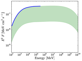
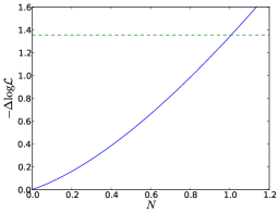
Figure 7: Left: Predicted $\gamma$-ray energy spectrum for SN 2010jl assuming $\Gamma_{p}=-2$ and a normalization of the $\gamma$-ray flux yielding $0.01<L_{\gamma}/L_{R}<0.1$ shown as the green shaded region compared to the $95\%$ flux upper limit (blue). Right: Likelihood profile for the spectral normalization parameter $N$ relative to the flux prediction yielding $L_{\gamma}/L_{R}=0.1$. The dashed green line indicates an increase of the negative delta log-likelihood by 2.71/2 compared to its minimum.

More stringent limits are expected from the joint likelihood results. Generic $\gamma$-ray flux predictions for various proton spectral indices are shown in Fig. 8. We calculate the $95\%$ CL upper limit on the $\gamma$-ray luminosity

$$L_{\gamma}=4\pi d^{2}F_{\gamma}^{I}=4\pi(10\,\textrm{Mpc})^{2}\frac{F_{\gamma}^{I}}{w_{d}},$$ (6)

where $F_{\gamma}^{I}$ is the integrated $\gamma$-ray flux over the energy range used in this analysis. The luminosity $L_{\gamma}$ is proportional to the result of the joint likelihood analysis using the weight $w_{d}=(10\,\textrm{Mpc}/d)^{2}$, assuming all sources have the same $L_{\gamma}$. In other words our joint likelihood results set a limit on $F_{\gamma}^{I}/w_{d}$ and thus on $L_{\gamma}$. The result is shown in Fig. 9 (left) as a function of the proton spectral index.

In addition we calculate the $95\%$ CL upper limit on the ratio of $\gamma$-ray to optical luminosity

$$L_{\gamma}/L_{R}=\frac{4\pi d^{2}F_{\gamma}^{I}}{L_{\sun}10^{0.4(M_{\sun}-M)}}=\frac{4\pi(1\,\textrm{Mpc})^{2}}{L_{\sun}10^{0.4M_{\sun}+4.8}}\frac{F_{\gamma}^{I}}{w_{m}},$$ (7)

where $L_{\sun}=6\times 10^{32}$ erg s^-1 is the R-band luminosity and $M_{\sun}=4.7$ the absolute $R$-band magnitude of the Sun. The ratio is proportional to $F_{\gamma}/w_{m}$, which is constrained by the joint likelihood analysis assuming a correlation of optical and $\gamma$-ray flux, i.e. weighting with $w_{m}=10^{-0.4m+5.2}$. Thus we can use the joint likelihood results to set a limit on $L_{\gamma}/L_{R}$ as a function of $\Gamma_{p}$ (see Fig. 9 right).

In Fig. 9 both limits discussed above are compared to the limit obtained using only one SN. The closest SN (SN 2011ht with a distance of $d=17.7$ Mpc) in the case of $1/d^{2}$ weighting and the brightest SN (SN 2010jl with a magnitude of $m=13.2$) in case of weighting with the optical flux. In both cases the combined limit is dominated by one SN. In the case of $1/d^{2}$ weighting the single source limit is better than the combined limit, indicating a statistical under-fluctuation in the individual analysis of this source or an over-fluctuation in one of the sources included in the joint likelihood.

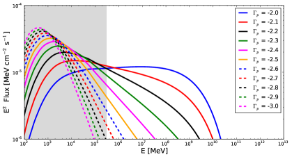
Figure 8: Gamma-ray energy spectra assuming a total $\gamma$-ray energy of $10^{50}$ erg, a source distance of $10$ Mpc and a duration of 1 year for various proton spectral indices $\Gamma_{p}$. The shaded grey region shows the energy range covered by this analysis.

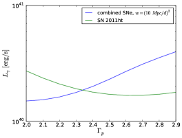
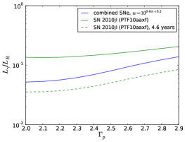
Figure 9: Left: $95\%$ CL upper limit on the $\gamma$-ray luminosity as a function of the proton spectral index based on the results obtained from the joint likelihood analysis with $1/d^{2}$ weighting shown in blue compared to the limit obtained from the closest single source SN 2011ht in green. Right: $95\%$ CL upper limit on the ratio of $\gamma$-ray and optical luminosity $L_{\gamma}/L_{R}$ as a function of $\Gamma_{p}$ assuming a proportionality between optical and $\gamma$-ray flux shown in blue compared to the limit obtained from a single source analysis of SN 2010jl considering a one year time window (in green). The results of the analysis with an extended time window of 4.5 years for SN 2010jl are shown in dashed green.

5 Conclusions

The origin of the multi-wavelength emission of Type IIn SNe and the onset of cosmic-ray production in supernova remnants is not fully understood. Type IIn SNe are expected to be host sites of particle acceleration, which could be pinpointed by transient $\gamma$-ray signals. For the first time we searched in a systematic way for $\gamma$-ray emission from a large ensemble of Type IIn SNe in coincidence with optical signals. No evidence for a signal was found, but our observational limits start to reach interesting parameter ranges expected by the theory. We set stringent limits on the $\gamma$-ray luminosity and the ratio of $\gamma$-ray and optical luminosity. For example, we can exclude $L_{\gamma}/L_{R}>0.1$ at $95\%$ CL for proton spectral indices of $<2.7$ from the results of the combined likelihood analysis assuming that $L_{\gamma}/L_{R}$ is constant. Those constraints can be converted to limits on the proton acceleration efficiency. In the case of SN 2010jl, our limits are close to theoretically expected values. However, uncertainties in the modeling, including the $\gamma$-ray escape fraction, leads to the range of $O(10\%)$ to $O(1\%)$ for the ratio of $\gamma$-ray to optical luminosity. Model-dependent calculations based on multi-wavelength observations will be performed in a future work and will allow us to set stringent constraints on the proton acceleration efficiency.

We do not have to make this assumption in the analysis of individual SNe. The results from the optically brightest SN in our sample, SN 2010jl, alone leads to only a factor of two weaker constraints, excluding $L_{\gamma}/L_{R}>0.2$. Assuming a scaling of the $\gamma$-ray flux with $1/d^{2}$ we can exclude $L_{\gamma}>4\times 10^{40}$ erg s^-1 at $95\%$ CL for all indices considered. A total $\gamma$-ray luminosity of $10^{50}$ erg emitted within 1 year (as assumed in Fig. 8) is excluded. The limits presented here are based on minimal assumptions about the $\gamma$-ray production and can be used to test various models.

6 Acknowledgements

The Fermi-LAT Collaboration acknowledges generous ongoing support from a number of agencies and institutes that have supported both the development and the operation of the LAT as well as scientific data analysis. These include the National Aeronautics and Space Administration and the Department of Energy in the United States, the Commissariat à l’Energie Atomique and the Centre National de la Recherche Scientifique / Institut National de Physique Nucléaire et de Physique des Particules in France, the Agenzia Spaziale Italiana and the Istituto Nazionale di Fisica Nucleare in Italy, the Ministry of Education, Culture, Sports, Science and Technology (MEXT), High Energy Accelerator Research Organization (KEK) and Japan Aerospace Exploration Agency (JAXA) in Japan, and the K. A. Wallenberg Foundation, the Swedish Research Council and the Swedish National Space Board in Sweden.

Additional support for science analysis during the operations phase is gratefully acknowledged from the Istituto Nazionale di Astrofisica in Italy and the Centre National d’Études Spatiales in France.

This paper is based on observations obtained with the Samuel Oschin Telescope as part of the Palomar Transient Factory project, a scientific collaboration between the California Institute of Technology, Columbia University, Las Cumbres Observatory, the Lawrence Berkeley National Laboratory, the National Energy Research Scientific Computing Center, the University of Oxford, and the Weizmann Institute of Science. Some of the data presented herein were obtained at the W. M. Keck Observatory, which is operated as a scientific partnership among the California Institute of Technology, the University of California, and NASA; the Observatory was made possible by the generous financial support of the W. M. Keck Foundation. We are grateful for excellent staff assistance at Palomar, Lick, and Keck Observatories. E.O.O. is incumbent of the Arye Dissentshik career development chair and is grateful to support by grants from the Willner Family Leadership Institute Ilan Gluzman (Secaucus NJ), Israeli Ministry of Science, Israel Science Foundation, Minerva and the I-CORE Program of the Planning and Budgeting Committee and The Israel Science Foundation. A. G.-Y. is supported by the EU/FP7 via ERC grant No. 307260, the Quantum Universe I-Core program by the Israeli Committee for planning and budgeting and the ISF, Minerva and ISF grants, WIS-UK “making connections”, and Kimmel and ARCHES awards.

Appendix A SN Catalog

The following table contains all SNe included in this analysis. The column definition is similar to Table 2.

Name	RA (∘)⋆	Dec (∘)⋆	Date	z	m	TS (p-value)
SN2008gm	348.55	-2.78	2008-10-22†	0.012	17.00‡	3.2 (0.169)
CSS081201_103354-032125	158.47	-3.36	2008-12-01†	0.060	18.30‡	0.0 (0.572)
CSS080701_234413+075224	356.05	7.87	2008-12-30	0.069	18.50	0.0 (0.572)
SN2008ja
SN2008ip	194.46	36.38	2008-12-31†	0.015	15.70‡	0.0 (0.572)
SN2009au	194.94	-29.60	2009-03-11†	0.009	16.40‡	0.0 (0.572)
CSS080928_160837+041626	242.16	4.27	2009-03-21	0.041	17.60	0.3 (0.458)
SN2008iy
SN2009cw	226.26	48.67	2009-03-28†	0.150	20.30‡	0.0 (0.572)
SN2009eo	224.53	2.43	2009-05-13†	0.044	18.10‡	0.0 (0.572)
SN2009fs	274.80	42.81	2009-06-01†	0.054	17.00‡	3.5 (0.154)
PTF09ij	218.06	54.86	2009-06-03	0.124	20.30	0.0 (0.572)
PTF09ge	224.26	49.61	2009-06-06	0.064	17.90	3.3 (0.165)
PTF09tm	206.73	61.55	2009-06-25	0.034	16.80	0.0 (0.572)
PTF09uj	215.05	53.56	2009-06-26	0.066	18.20	0.0 (0.572)
PTF09uy	190.98	74.69	2009-07-03	0.313	19.40	0.0 (0.572)
PTF09bcl	271.61	17.86	2009-07-19†	0.062	20.87‡	0.0 (0.572)
PTF10ujc	353.63	22.35	2009-08-05	0.032	16.20	0.0 (0.572)
PTF09drs	226.63	60.59	2009-08-15	0.045	18.50	0.0 (0.561)
CSS090925_001259+144121	3.25	14.69	2009-09-25†	0.090	18.80‡	0.0 (0.568)
SN2009ma	127.24	0.59	2009-10-17†	0.089	18.20‡	0.0 (0.572)
CSS091018_091109+195945	137.79	20.00	2009-10-18†	0.150	19.00‡	0.0 (0.572)
SN2009mb
SN2009kn	122.43	-17.75	2009-10-26†	0.016	16.60‡	0.0 (0.572)
SN2009kr	78.01	-15.70	2009-11-06†	0.006	16.00‡	4.7 (0.104)
SN2009nm	151.35	51.28	2009-11-20†	0.210	18.80‡	0.0 (0.572)
CSS091217_110637+341952	166.65	34.33	2009-12-17†	?	18.70‡	0.0 (0.572)
SN2009nj
CSS091218_104011+223735	160.05	22.63	2009-12-18†	0.140	19.40‡	0.0 (0.572)
SN2009nw
PTF10dk	77.09	0.21	2009-12-18†	0.074	20.14‡	0.0 (0.572)
PTF10u	152.49	46.01	2010-01-05	0.150	19.80	0.0 (0.572)
PTF11ner	125.58	72.83	2010-01-11†	0.117	20.94‡	0.0 (0.572)
PTF10ts	188.49	13.92	2010-01-12	0.046	17.66	7.9 (0.033)
SN2009nn
CSS100113_032138+263650	50.41	26.61	2010-01-13†	0.060	18.80‡	0.1 (0.517)
SN2010M
PTF10cwl	189.09	7.79	2010-03-13†	0.085	19.00‡	0.0 (0.572)
SN2010al	123.57	18.44	2010-03-13†	0.017	17.80‡	9.7 (0.023)
PTF10cwx	188.32	-0.05	2010-03-19	0.073	18.50	2.3 (0.228)
PTF10fei	227.07	53.59	2010-04-04	0.090	18.55	0.0 (0.572)
PTF10fel	246.88	51.36	2010-04-04	0.234	19.70	11.1 (0.016)
PTF10ewc	210.50	33.84	2010-04-15	0.055	18.40	0.3 (0.476)
PTF10fou	208.94	29.88	2010-04-17	0.043	20.00	0.2 (0.489)
PTF10flx	251.74	64.45	2010-04-17	0.067	18.80	11.6 (0.015)
SN2010bt	192.08	-34.95	2010-04-17†	0.016	15.80‡	14.4 (0.0065)
PTF10fjh	251.73	34.16	2010-04-25	0.032	17.20	0.0 (0.572)
SN2010bq
PTF10gvd	253.26	67.00	2010-05-02	0.070	19.20	2.8 (0.196)
PTF10hcr	183.00	38.53	2010-05-06†	0.037	20.06‡	1.0 (0.359)
PTF10hbf	193.19	-6.92	2010-05-07	0.042	18.80	0.6 (0.407)
PTF10hif	257.45	27.26	2010-05-12	0.141	18.00	0.0 (0.572)
PTF10gvf	168.44	53.63	2010-05-14	0.080	19.00	0.0 (0.572)
PTF10hSN	244.40	5.04	2010-06-01	0.164	19.00	0.0 (0.572)
PTF10jop	322.38	2.88	2010-06-11	0.089	18.60	0.0 (0.572)
PTF10ngx	186.80	15.98	2010-07-03	0.067	19.40	0.0 (0.572)
PTF10ndr	224.95	65.00	2010-07-26	0.075	19.60	0.0 (0.572)
PTF10qaf	353.93	10.78	2010-07-31	0.284	19.00	7.5 (0.036)
SN2010hd	340.47	-46.10	2010-08-07†	0.033	17.60‡	8.8 (0.028)
PS1-1000789	310.69	15.51	2010-08-15†	0.200	17.30‡	0.0 (0.572)
PTF10oug	260.19	29.07	2010-08-20	0.150	19.20	0.0 (0.572)
PTF10scc	352.04	28.64	2010-08-20	0.242	18.90	0.0 (0.572)
PTF10qwu	252.79	28.30	2010-08-20	0.226	19.40	0.1 (0.541)
PTF10tjr	220.38	23.01	2010-08-23†	0.078	17.73‡	0.0 (0.572)
PTF10tpz	329.63	-15.55	2010-08-28†	0.040	17.06‡	0.0 (0.572)
PTF10tel	260.38	48.13	2010-09-04	0.035	17.50	0.0 (0.572)
SN2010mc
PTF10ttp	341.92	-10.04	2010-09-09	0.179	19.50	0.0 (0.572)
CSS100910_001539+271250	3.91	27.21	2010-09-10†	0.024	18.10‡	0.0 (0.572)
PTF10viv	331.11	-7.98	2010-09-12†	0.060	20.13‡	0.0 (0.572)
SN2010jg
PTF10uls	20.34	4.89	2010-09-19	0.044	18.60	1.4 (0.322)
PTF10xzs	120.60	67.42	2010-09-22†	0.036	19.33‡	8.2 (0.031)
PTF10wop	327.65	-6.77	2010-09-23†	0.090	19.55‡	0.0 (0.572)
PTF10xif	48.11	-9.81	2010-09-27†	0.029	18.42‡	0.0 (0.572)
PTF10vag	326.83	18.13	2010-09-29	0.052	18.50	0.0 (0.572)
PTF10xgo	328.99	1.32	2010-10-03†	0.034	19.25‡	2.8 (0.193)
CSS121009_025917-141610	44.82	-14.27	2010-10-09†	0.080	19.20‡	0.0 (0.572)
PTF10tyd	257.33	27.82	2010-10-09	0.063	19.00	0.0 (0.572)
PTF12kph	24.82	-7.56	2010-10-11†	0.059	18.84‡	6.1 (0.063)
PTF10uiz	258.63	21.43	2010-10-19	0.114	18.40	0.0 (0.572)
PTF10wmk	132.04	55.83	2010-10-29	0.137	19.51	0.0 (0.572)
PTF10yzt	2.96	26.69	2010-10-29†	0.076	18.58‡	0.0 (0.572)
CSS101030_230944+054156	347.43	5.70	2010-10-30†	0.042	16.50‡	0.0 (0.572)
SN2010jy
PTF10aaes	31.79	16.21	2010-10-30†	0.037	19.50‡	0.0 (0.572)
SN2010jk	18.15	15.47	2010-10-31†	0.280	20.20‡	3.6 (0.153)
PTF10acfd	147.91	1.52	2010-11-03†	0.192	20.34‡	0.0 (0.572)
SN2010lx	71.19	-22.21	2010-11-03†	0.100	18.70‡	0.0 (0.572)
SN2010js	124.21	60.50	2010-11-07†	0.039	18.10‡	1.9 (0.262)
PTF10yyc	69.82	-0.35	2010-11-08	0.214	17.66	0.9 (0.367)
PTF10weh	261.71	58.85	2010-11-08	0.138	18.30	6.6 (0.048)
CSS101110_082047+355337	125.20	35.89	2010-11-10†	0.075	18.20‡	6.2 (0.059)
2010kb
PTF10aazn	31.72	44.57	2010-11-13†	0.016	16.52‡	5.4 (0.079)
SN2010jj
PTF10aaxf	145.72	9.50	2010-11-18	0.011	13.20	7.1 (0.039)
SN2010jl
PTF10abcl	348.90	22.81	2010-11-19†	0.061	18.95‡	3.0 (0.181)
PTF10aaxi	94.13	-21.41	2010-11-23	0.010	18.00	0.0 (0.572)
SN2010jp
PTF10yni	2.71	14.18	2010-11-28	0.169	18.90	7.2 (0.039)
PTF10abui	93.08	-22.77	2010-12-08	0.052	18.60	0.0 (0.572)
PTF10abyy	79.17	6.80	2010-12-08†	0.030	18.66‡	0.2 (0.503)
PTF10achk	46.49	-10.52	2010-12-28	0.033	16.90	0.0 (0.572)
SN2011A	195.25	-14.53	2011-01-02†	0.009	16.90‡	0.0 (0.572)
SN2011P	36.44	16.22	2011-01-05†	0.080	18.60‡	10.8 (0.016)
SN2011af	36.48	10.39	2011-01-11†	0.064	16.70‡	0.0 (0.572)
SN2011S	138.48	-17.01	2011-01-14†	0.060	17.60‡	0.0 (0.572)
PTF10acsq	120.39	46.76	2011-01-27	0.173	19.00	0.0 (0.572)
SN2011ap	272.62	31.01	2011-02-21†	0.024	18.30‡	0.0 (0.572)
SN2011an	119.85	16.42	2011-03-01†	0.016	18.40‡	0.7 (0.398)
SN2011cc	248.46	39.26	2011-03-17†	0.032	17.70‡	0.0 (0.572)
PS1-11xn	221.91	51.68	2011-04-26†	0.040	18.60‡	0.0 (0.572)
SN2011cp	118.14	21.89	2011-04-26†	0.390	19.50‡	5.4 (0.081)
CSS110501_094825+204333	147.10	20.73	2011-05-01†	0.040	18.40‡	0.0 (0.572)
PTF11csc	224.68	36.60	2011-05-02	0.117	20.60	0.0 (0.572)
PTF11dsb	244.65	32.70	2011-05-15	0.190	20.10	0.0 (0.572)
SN2011eu	212.31	-1.18	2011-06-06†	0.110	18.50‡	0.0 (0.572)
PTF11fuu	325.12	6.33	2011-06-09	0.097	18.50	0.0 (0.572)
PTF11fss	323.47	1.84	2011-06-11†	0.125	19.42‡	0.0 (0.572)
CSS110623_131919-045106	199.83	-4.85	2011-06-23†	0.070	18.40‡	0.0 (0.572)
PTF11gtr	258.01	23.38	2011-06-25†	0.029	20.94‡	0.0 (0.572)
PTF11hzx	327.67	18.11	2011-07-24	0.229	18.90	0.0 (0.572)
PTF11iqb	8.52	-9.70	2011-08-06	0.013	15.20	0.3 (0.469)
PTF11fzz	167.69	54.11	2011-08-15	0.082	17.40	0.3 (0.479)
SN2011fh	194.06	-29.50	2011-08-24†	0.008	14.50‡	1.9 (0.262)
PTF11pab	44.63	6.31	2011-08-30†	0.022	21.08‡	6.1 (0.063)
SN2011fx	4.50	24.56	2011-08-30†	0.019	17.60‡	0.5 (0.428)
SN2011fr	22.44	18.89	2011-09-01†	0.060	18.80‡	0.0 (0.572)
PTF11mpg	334.40	0.61	2011-09-19	0.093	19.18	0.0 (0.572)
PTF11oey	352.73	23.18	2011-09-21†	0.061	20.17‡	0.0 (0.572)
PTF11mtq	270.08	28.70	2011-09-22†	0.073	19.35‡	1.6 (0.302)
PTF11msk	325.91	-1.69	2011-10-04	0.070	19.10	2.2 (0.238)
PTF11pdt	44.63	6.31	2011-10-19†	0.022	20.00‡	8.9 (0.028)
PSNJ10081059+5150570	152.04	51.85	2011-10-29	0.004	14.50	0.0 (0.572)
SN2011ht
PTF11qnf	86.23	69.15	2011-11-01†	0.014	19.80‡	1.4 (0.320)
SN2011ib	176.16	35.97	2011-11-15†	0.037	16.80‡	0.0 (0.572)
SN2011hw	336.56	34.22	2011-11-18†	0.023	15.70‡	0.0 (0.572)
SN2011jb	174.27	15.47	2011-11-28†	0.084	17.80‡	0.0 (0.572)
SN2011iw	353.70	24.75	2011-11-29†	0.023	16.90‡	0.0 (0.572)
PTF11qqj	149.51	0.72	2011-12-11	0.093	19.00	0.0 (0.572)
PTF11oxu	54.64	22.55	2011-12-13	0.088	18.70	4.7 (0.103)
SN2011jc
PTF11rlv	192.39	-9.34	2011-12-21†	0.132	19.77‡	0.0 (0.572)
PTF11rfr	25.57	29.27	2011-12-23	0.067	17.30	0.0 (0.572)
PTF12th	72.62	-3.49	2012-01-05†	0.084	19.08‡	0.0 (0.572)
SN2012Y
PTF12xv	70.20	6.52	2012-01-18†	0.120	19.51‡	0.0 (0.572)
SN2012ab	185.70	5.61	2012-01-31†	0.018	15.80‡	0.0 (0.572)
SN2012as	231.29	37.96	2012-02-17†	0.029	17.90‡	0.0 (0.572)
SN2012al	151.55	47.29	2012-02-24†	0.040	18.10‡	0.7 (0.398)
SN2012am	163.51	46.03	2012-02-24†	0.042	17.60‡	0.0 (0.572)
LSQ12biu	214.84	-19.84	2012-03-21†	0.136	19.40‡	1.1 (0.352)
CSS120327_110520-015205	166.33	-1.87	2012-03-27†	0.090	17.80‡	0.0 (0.572)
CSS120330_101639-064636	154.16	-6.78	2012-03-28†	0.042	17.30‡	0.0 (0.572)
LSQ12by
PTF11mhr	236.51	31.94	2012-03-28	0.054	17.30	0.4 (0.451)
LSQ12bqd	197.91	-16.40	2012-03-29†	0.041	19.30‡	0.0 (0.572)
SN2012bq	154.16	-6.78	2012-03-30†	0.042	17.60‡	0.0 (0.572)
PTF12cix	191.29	35.94	2012-04-01	0.190	19.50	0.0 (0.572)
PTF12csy	104.64	17.26	2012-04-07†	0.067	19.20‡	0.0 (0.572)
LSQ12btw	152.62	5.54	2012-04-09†	0.057	19.10‡	0.0 (0.572)
PSNJ18410706-4147374	280.28	-41.79	2012-04-25†	0.019	14.50‡	0.0 (0.572)
SN2012ca
PTF12cxj	198.16	46.49	2012-04-28	0.035	18.70	0.0 (0.572)

Appendix B Likelihood Profiles in Energy Bins

Figures 10 and 11 show the likelihood profiles in energy bins for $\Delta T=1$ yr and the 95% CL upper limit for three time windows $\Delta T=1$ yr, $~{}\Delta T=6$ months and $\Delta T=3$ months for all SNe listed in Table 2.

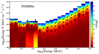
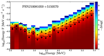
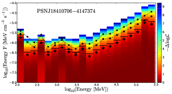
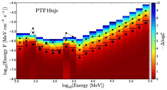
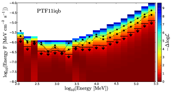
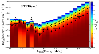
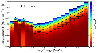
Figure 10: Similar to Fig. 4. Colors represent the likelihood profile for each energy for $\Delta T=1$ yr. The black arrows indicate the 95% CL upper limits for $\Delta T=1$ yr, while the dotted-dashed and dotted lines represent the 95% CL upper limit for $~{}\Delta T=6$ months and $\Delta T=3$ months respectively.

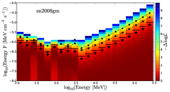
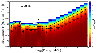
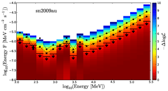
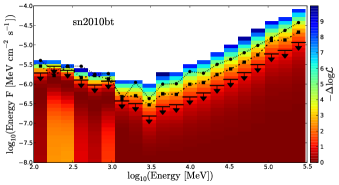
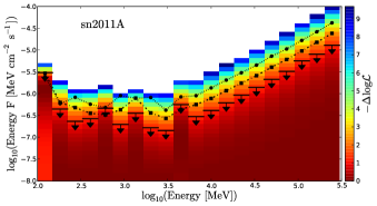
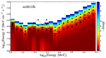
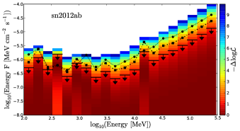
Figure 11: Similar to Fig. 4. Colors represent the likelihood profile for each energy for $\Delta T=1$ yr. The black arrows indicate the 95% CL upper limits for $\Delta T=1$ yr, while the dotted-dashed and dotted lines represent the 95% CL upper limit for $~{}\Delta T=6$ months and $\Delta T=3$ months respectively.

References

- Abdo et al. (2010) Abdo, A., Ackermann, M., Ajello, M., et al. 2010, Science, 329, 817
- Abdo et al. (2009) Abdo, A. A., Ackermann, M., Ajello, M., et al. 2009, ApJS, 183, 46
- Ackermann et al. (2014) Ackermann, M., Albert, A., Anderson, B., et al. 2014, Phys. Rev. D, 89, 042001
- Ade et al. (2014) Ade, P. A. R., Aghanim, N., Alves, M. I. R., et al. 2014, A&A, 571, A1
- Atwood et al. (2009) Atwood, W. B., Abdo, A. A., Ackermann, M., et al. 2009, ApJ, 697, 1071
- Bartlett (1953) Bartlett, M. 1953, Biometrika, 40, 306
- Bregeon et al. (2013) Bregeon, J., Charles, E., & Wood, M. 2013, ArXiv:1304.5456
- Cheung et al. (2013) Cheung, C.C, ., Jean, P., Shore, S., et al. 2013, ATel, 5649
- Chevalier & Irwin (2011) Chevalier, R. A., & Irwin, C. M. 2011, ApJ, 729, L6
- Cooke et al. (2009) Cooke, J., Sullivan, M., Barton, E. J., et al. 2009, Nature, 460, 237
- Fransson et al. (2014) Fransson, C., Ergon, M., Challis, P. J., et al. 2014, ApJ, 797, 118
- Hays et al. (2013) Hays, E., Cheung, T., & Ciprini, S. 2013, ATel, 5302
- Hill et al. (2013) Hill, A., Cheung, C., & Jean, P. 2013, proceedings of the 2013 Recontres de Moriond, 129
- Katz et al. (2011) Katz, B., Sapir, N., & Waxman, E. 2011, ArXiv:1106.1898
- Kelner et al. (2006) Kelner, S. R., Aharonian, F. A., & Bugayov, V. V. 2006, Phys. Rev. D, 74, 034018
- Law et al. (2009) Law, N. M., Kulkarni, S. R., Dekany, R. G., et al. 2009, PASP, 121, 1395
- Margutti et al. (2014) Margutti, R., Milisavljevic, D., Soderberg, A. M., et al. 2014, ApJ, 780, 21
- Murase et al. (2011) Murase, K., Thompson, T., Lacki, B., et al. 2011, Phys. Rev. D, 84, 043003
- Murase et al. (2014) Murase, K., Thompson, T., & Ofek, E. 2014, MNRAS, 440, 2528
- Neyman & Pearson (1928) Neyman, J., & Pearson, E. S. 1928, Biometrika, 20A, 175
- Nolan et al. (2012) Nolan, P. L., Abdo, A. A., Ackermann, M., et al. 2012, ApJS, 199, 31
- Ofek et al. (2007) Ofek, E. O., Cameron, P. B., Kasliwal, M. M., et al. 2007, ApJ, 659, L13
- Ofek et al. (2013) Ofek, E. O., Lin, L., Kouveliotou, C., et al. 2013, ApJ, 768, 47
- Ofek et al. (2010) Ofek, E. O., Rabinak, I., Neill, J. D., et al. 2010, ApJ, 724, 1396
- Ofek et al. (2014b) Ofek, E. O., Sullivan, M., Shaviv, N. J., et al. 2014b, ApJ, 789, 104
- Ofek et al. (2014a) Ofek, E. O., Zoglauer, A., Boggs, S. E., et al. 2014a, ApJ, 781, 42
- Quimby et al. (2011) Quimby, R. M., Kulkarni, S. R., Kasliwal, M. M., et al. 2011, Nature, 474, 487
- Rau et al. (2009) Rau, A., Kulkarni, S. R., Law, N. M., et al. 2009, PASP, 121, 1334
- Rolke et al. (2005) Rolke, W. A., López, A. M., & Conrad, J. 2005, Nuclear Instruments and Methods in Physics Research A, 551, 493
- Smith et al. (2009) Smith, N., Hinkle, K. H., & Ryde, N. 2009, AJ, 137, 3558
- Sveshnikova (2003) Sveshnikova, L. G. 2003, A&A, 409, 799
- Svirski et al. (2012) Svirski, G., Nakar, E., & Sari, R. 2012, ApJ, 759, 108
- Zhang et al. (2012) Zhang, T., Wang, X., Wu, C., et al. 2012, AJ, 144, 131