The Meta Distribution of the SIR
in Poisson Bipolar and Cellular Networks

Abstract

The calculation of the SIR distribution at the typical receiver (or, equivalently, the success probability of transmissions over the typical link) in Poisson bipolar and cellular networks with Rayleigh fading is relatively straightforward, but it only provides limited information on the success probabilities of the individual links.

This paper introduces the notion of the meta distribution of the SIR, which is the distribution of the conditional success probability $P_{\rm s}$ given the point process, and provides bounds, an exact analytical expression, and a simple approximation for it. The meta distribution provides fine-grained information on the SIR and answers questions such as “What fraction of users in a Poisson cellular network achieve 90% link reliability if the required SIR is 5 dB?”.

Interestingly, in the bipolar model, if the transmit probability $p$ is reduced while increasing the network density $\lambda$ such that the density of concurrent transmitters $\lambda p$ stays constant as $p\to 0$, $P_{\rm s}$ degenerates to a constant, i.e., all links have exactly the same success probability in the limit, which is the one of the typical link. In contrast, in the cellular case, if the interfering base stations are active independently with probability $p$, the variance of $P_{\rm s}$ approaches a non-zero constant when $p$ is reduced to $0$ while keeping the mean success probability constant.

I Introduction

I-A Motivation

Stochastic geometry provides the tools to analyze wireless networks with randomly placed nodes. A key quantity of interest in interference-limited networks is the success probability $p_{\rm s}(\theta)\triangleq\mathbb{P}(\mathsf{SIR}>\theta)$ of the transmission over the typical link, which corresponds to the complementary cumulative distribution (ccdf) of the signal-to-interference ratio (SIR). The calculation of $p_{\rm s}$ involves spatial averaging, i.e., the evaluation of a certain expectation over the point process. While this expected value is certainly important, it does not reveal how concentrated the link success probabilities are. For example, in one network model, all links (or users) could have success probabilities between $0.85$ and $0.95$, while in another, some links may have $0.5$ and some may have $0.99$. In both cases, we may find $p_{\rm s}=0.9$, but the performances of the two networks in terms of connectivity, end-to-end delay, or quality-of-experience would differ greatly. Hence it is important to quantify the variability of the link reliabilities around $p_{\rm s}$.

To this end, our focus in this paper are random variables of the form

$$P_{\rm s}(\theta)\triangleq\mathbb{P}(\mathsf{SIR}>\theta\mid\Phi,\mathsf{tx}),$$ (1)

where the conditional probability is taken over the fading and the channel access scheme (if random) of the interferers given the point process and given that the desired transmitter is active. The goal is to find (or bound) the ccdf of $P_{\rm s}$, defined as

$$\bar{F}_{P_{\rm s}}(x)\triangleq\mathbb{P}^{!{\rm t}}(P_{\rm s}(\theta)>x),\quad x\in[0,1],$$ (2)

where $\mathbb{P}^{!{\rm t}}$ denotes the reduced Palm measure of the point process, given that there is an active transmitter at the prescribed location. Since $\bar{F}_{P_{\rm s}}$ is the (complementary) distribution of a conditional probability, we call it the meta distribution of the SIR. Using this notation, the standard success probability is the mean

$$p_{\rm s}(\theta)=\mathbb{E}^{!{\rm t}}(P_{\rm s}(\theta))=\int_{0}^{1}\bar{F}_{P_{\rm s}}(x)\mathrm{d}x.$$

While a direct calculation of the ccdf (2) seems infeasible, we shall see that the moments of $P_{\rm s}(\theta)$ can be expressed in closed-form, which allows the derivation of an exact analytical expression and simple bounds. The $b$-th moment of $P_{\rm s}(\theta)$ is denoted by $M_{b}$, i.e., we define

$$M_{b}(\theta)\triangleq\mathbb{E}^{!{\rm t}}(P_{\rm s}(\theta)^{b})=\int_{0}^{1}bx^{b-1}\bar{F}_{P_{\rm s}}(x)\mathrm{d}x.$$

Hence we have $p_{\rm s}(\theta)\equiv M_{1}(\theta)$.

I-B Contributions

The contributions of the paper are:

• We introduce the meta distribution of the SIR.

• We give closed-form expression of the moments $M_{b}$ for Poisson bipolar networks with ALOHA and for Poisson cellular networks, both for Rayleigh fading.

• We provide an analytical expression for the exact meta distribution for the two types of networks.

• We propose the beta distribution as a highly accurate approximation.

• We show that, remarkably, in the limit of very dense bipolar networks with small transmit probability, all links have the same success probability. This is not the case in cellular networks with random (interfering) base station activity, since the variance $M_{2}-M_{1}^{2}$ is bounded away from zero when the probability of a base station being active goes to $0$.

• We give the conditions on the SIR threshold $\theta$ and the transmit probability $p$ for a finite mean local delay.

I-C Related work

The calculation of the (mean) success probability $p_{\rm s}(\theta)$ in Poisson bipolar networks is provided in [1] but can be traced back to [2]. In [3], the moments $M_{b}$ of the link success probabilities are calculated under the assumption of no MAC scheme (i.e., all nodes always transmit), and bounds on the distribution are obtained.

For Poisson cellular models, where the typical user is associated with the nearest base station (strongest base station on average), the result was derived in [4] and extended to the multi-tier Poisson case (HIP model) in [5].

The joint success probability of multiple transmissions in Poisson bipolar networks is calculated in [6]. Similarly, [7] determined the joint success probabilities of multiple transmissions (or transmissions over multiple resource blocks) for Poisson cellular networks. As we shall see, these joint probabilities are related to the integer moments $M_{k}$ of the conditional success probabilities.

I-D The meta distribution

In this section, we formally introduce the concept of a meta distribution, which is the distribution of the conditional distribution $P_{\rm s}$.

Definition 1 (Meta distribution)

The meta distribution of the SIR is the two-parameter distribution function

$$\bar{F}(\theta,x)\triangleq\bar{F}_{P_{\rm s}}(\theta,x)=\mathbb{P}^{!{\rm t}}(P_{\rm s}(\theta)>x),\quad\theta\in\mathbb{R}^{+},\>x\in[0,1].$$

We have $\bar{F}(0,x)=1$ for $x<1$, $\lim_{\theta\to\infty}\bar{F}(\theta,x)=0$ for $x>0$, $\bar{F}(\theta,0)=1$, and $\bar{F}(\theta,1)=0$. For fixed $\theta$, it is a standard ccdf and yields the probability that the typical link or user achieves an SIR of $\theta$ or, equivalently, the fraction of links or users (assuming a uniform user distribution) that achieve this SIR. Generally, it yields the fraction of links or users that achieve an SIR of $\theta$ with probability at least $x$.

In the next two sections, we will calculate the meta distribution and bounds for Poisson bipolar and cellular networks, respectively.

II Poisson Bipolar Networks

II-A System Model

We consider the Poisson bipolar model [8, Def. 5.8], where the (potential) transmitters form a Poisson point process (PPP) $\Phi$ of intensity $\lambda$ and each one has a dedicated receiver at distance $R$ in a random orientation. In each time slot, nodes in $\Phi$ independently transmit with probability $p$, and all channels are subject to Rayleigh fading.

We use the standard path loss model with exponent $\alpha$, define $\delta\triangleq 2/\alpha$, and we let $C\triangleq\lambda\pi R^{2}\Gamma(1-\delta)\Gamma(1+\delta)$ be a coefficient that does not depend on $\theta$. The success probability of the typical link is well known, see, e.g., [1, 9, 8], and can be expressed as

$$p_{\rm s}(\theta)\triangleq\mathbb{P}^{!{\rm t}}(\mathsf{SIR}>\theta)=M_{1}(\theta)=e^{-C\theta^{\delta}p}.$$

Due to the ergodicity of the PPP, the ccdf of $P_{\rm s}$ can be alternatively written as the limit

$$\bar{F}_{P_{\rm s}}(x)=\lim_{r\to\infty}\frac{1}{\lambda p\pi r^{2}}\sum_{\begin{subarray}{c}y\in\Phi\\ \|y\|<r\end{subarray}}\mathbf{1}(\mathbb{P}(\mathsf{SIR}_{\tilde{y}}>\theta\mid\Phi)>x),$$

where $\tilde{y}$ is the receiver of transmitter $y$ and $\mathbf{1}(\cdot)$ is the indicator function. This shows that $\bar{F}_{P_{\rm s}}(x)$ denotes the fraction of links in the network (in each realization of the point process) that, when scheduled to transmit, have a success probability larger than $x$.

The link success probabilities for a given realization can also be “attached” to each point of the transmitter process $\Phi$ to form a marked point process $\hat{\Phi}=\{(x_{i},P_{\rm s}^{x_{i}})\}$. The meta distribution can then be interpreted as the mark distribution, parametrized by $\theta$. Due to the interference correlation [10], the marks of nearby nodes are correlated, hence $\hat{\Phi}$ is not an independently marked process.

Fig. 1 shows an example realization of a Poisson bipolar network together with the success probabilities for each link, averaged over the fading and ALOHA. As expected, links whose receivers are relatively isolated from interfering transmitters have a high success rate, while those in crowded parts of the network suffer from a low one.

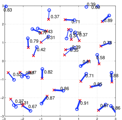
Figure 1: Realization of a Poisson bipolar network for $\lambda=1$, $R=1/2$, $p=1/2$, $\theta=1$, $\alpha=4$, resulting in $p_{\rm s}=0.54$. The number next to each link is its success probability (averaged over fading and ALOHA).

II-B Moments

Let

$$D_{b}(p,\delta)\triangleq\sum_{k=1}^{\infty}\binom{b}{k}\binom{\delta-1}{k-1}p^{k},\quad b\in\mathbb{C}\text{ and }p,\delta\in[0,1].$$ (3)

For $p=1$,

$$D_{b}(1,\delta)=\frac{\Gamma(b+\delta)}{\Gamma(b)\Gamma(1+\delta)},$$

which is not defined if $b\in\mathbb{Z}^{-}$ or $b+\delta\in\mathbb{Z}^{-}$. For $\delta\in\{0,1\}$, the function simplifies to $D_{b}(p,0)=1-(1-p)^{b}$ and $D_{b}(p,1)=bp$.

Alternatively, the function can be expressed using the Gaussian hypergeometric function ${}_{2}F_{1}$ as

$$D_{b}(p,\delta)=pb\>_{2}F_{1}(1-b,1-\delta;2;p).$$ (4)

Theorem 1 (Moments for bipolar network with ALOHA)

Given that the typical link is active, the moment $M_{b}$ of the conditional success probability is

$$M_{b}(\theta)=\exp\left(-C\theta^{\delta}D_{b}(p,\delta)\right),\quad b\in\mathbb{C},$$ (5)

whenever $D_{b}(p,\delta)$ is defined.

Proof: See Appendix A.

An important and helpful observation in the proof is that the calculation of the $n$-th moment for $n\in\mathbb{N}$ is the same as that of the joint success probability of $n$ transmissions, calculated in [6]. In this case, $D_{n}(p,\delta)$ is given by the finite sum

$$D_{n}(p,\delta)=\sum_{k=1}^{n}\binom{n}{k}\binom{\delta-1}{k-1}p^{k},$$

which is a polynomial of degree $n$ in $p$ and degree $n-1$ in $\delta$ and called the diversity polynomial in [6, Def. 1].

Since (5) is valid for (essentially) any $b\in\mathbb{C}$, we can use it to obtain the $-1$-st moment as

$$M_{-1}(\theta) =\exp(C\theta^{\delta}p(1-p)^{\delta-1})$$

$$=M_{1}^{-(1-p)^{\delta-1}},\quad p<1.$$ (6)

$M_{-1}$ is the mean number of transmission attempts needed to succeed once if the transmitter is allowed to keep transmitting until success. This quantity is termed mean local delay and is calculated in [11, Lemma 2]. Noteworthy is the phase transition at $p=1$. For $p=1-\epsilon$, the mean local delay is finite for all $\epsilon>0$. But if all nodes always transmit, it is infinite.

An interesting question is what happens when $p\to 0$ while the transmitter density $p\lambda$ (and thus $M_{1}$) is kept constant. It is answered in the following corollary.

Corollary 1 (Concentration as $p\to 0$)

Denoting the transmitter density as $\tau\triangleq\lambda p$ and keeping it (and thus $M_{1}$) fixed while letting $p\to 0$, we have

$$\lim_{\begin{subarray}{c}p\to 0\\ \lambda p=\tau\end{subarray}}P_{\rm s}(\theta)=p_{\rm s}(\theta)$$

in mean square (and probability and distribution).

Proof:

From (5), the second moment is

$$M_{2}(\theta)=e^{-C\theta^{\delta}(2p+(\delta-1)p^{2})},$$

and the variance, expressed in terms of $M_{1}$ (which is kept constant), is

$$\operatorname{var}P_{\rm s}(\theta)=M_{1}^{2}(M_{1}^{p(\delta-1)}-1).$$ (7)

It follows that

$$\lim_{\begin{subarray}{c}p\to 0\\ \lambda p=\tau\end{subarray}}\operatorname{var}P_{\rm s}(\theta)=0.$$

∎

So if $C\theta^{\delta}p$ is kept constant, the variance can be adjusted by changing $p$. For example, if $C=1/(10p\theta^{\delta})$, $M_{1}=e^{-1/10}\approx 0.9$, and the variance can be reduced to $0$ by letting $p\to 0$. So, counterintuitively, a small $p$ decreases the variance and, in the limit, all links in the network have exactly the same success probability.

More precisely, the variance is proportional to $p$ for small $p$ if $M_{1}$ is kept constant:

$$\operatorname{var}P_{\rm s}(\theta)\sim-M_{1}^{2}\log(M_{1})(1-\delta)p,\quad p\to 0.$$

The next result provides tight bounds on the moments if $p=1$ for $b\in\mathbb{R}^{+}$. ${}^{\prime}\!\!\lesssim^{\prime}$ and ${}^{\prime}\!\!\gtrsim^{\prime}$ indicate upper bound and lower bounds with asymptotic equality (here as $b\to\infty$), respectively.

Corollary 2 (Bounds on moments for $p=1$)

For $b>0$,

$$M_{b}=M_{1}^{\frac{\Gamma(b+\delta)}{\Gamma(1+\delta)\Gamma(b)}}\gtrsim\exp(-C\theta^{\delta}b^{\delta}),$$ (8)

for $b\geq 1$,

$$M_{b}\leq M_{1}^{b^{\delta}},$$ (9)

and for $0<b<1$,

$$M_{b}>M_{1}^{b^{\delta}}.$$ (10)

Proof:

The lower bound (8) follows from (5) by setting $p=1$ and the asymptotic bound $\Gamma(b+\delta)/\Gamma(b)\lesssim b^{\delta}$ for $b>0$. Conversely, $\Gamma(b+\delta)/\Gamma(b)\geq b^{\delta}\Gamma(1+\delta)$ for all $b\geq 1$, which yields the upper bound (9):

$$M_{b} \leq\exp(-Cb^{\delta}\Gamma(1+\delta))=M_{1}^{b^{\delta}},\quad b\geq 1.$$

For $b<1$, $\Gamma(b+\delta)/\Gamma(b)<b^{\delta}\Gamma(1+\delta)$, and the direction of the inequality is reversed, yielding (10). ∎

The third bound is tighter than the first one in the regime where it is valid. Further, since

$$M_{1}^{b^{\delta}}=\exp\left(-C(b\theta)^{\delta}\right),$$

the $b$-th moment is bounded by the first moment evaluated at $b\theta$, i.e.,

$$M_{b}(\theta)\leq M_{1}(b\theta),\quad b\geq 1,$$

and vice versa if $b<1$.

II-C Exact expression

An exact integral expression can be obtained from the purely imaginary moments $M_{jt}$, $t\in\mathbb{R}$, $j\triangleq\sqrt{-1}$.

Corollary 3 (Exact integral expression)

The meta distribution is given by

$$\bar{F}(\theta,x)=\frac{1}{2}-\frac{1}{\pi}\int_{0}^{\infty}\frac{e^{-C\theta^{\delta}\Re(D_{jt})}\sin(t\log x+C\theta^{\delta}\Im(D_{jt}))}{t}\mathrm{d}t,$$ (11)

where $D_{jt}=D_{jt}(p,\delta)$ is given in (3) and $\Re(z)$ and $\Im(z)$ denote the real and imaginary parts of the complex number $z$, respectively.

Proof:

Let $X\triangleq\log P_{\rm s}(\theta)$. The characteristic function of $X$ is

$$\varphi_{X}(t) \triangleq\mathbb{E}e^{jtX}=\mathbb{E}(P_{\rm s}(\theta)^{jt})=M_{jt},\quad t\in\mathbb{R}.$$

where $M_{jt}$ is given in (5). Then by the Gil-Pelaez theorem [12], the ccdf of $X$ is given by

$$\bar{F}_{X}(x)=\frac{1}{2}+\frac{1}{\pi}\int_{0}^{\infty}\frac{\Im(e^{-jtx}M_{jt})}{t}\mathrm{d}t.$$ (12)

Since $\mathbb{P}(P_{\rm s}(\theta)>x)=\mathbb{P}(\log P_{\rm s}(\theta)>\log x)$,

$$\bar{F}_{P_{\rm s}}(x) =\frac{1}{2}+\frac{1}{\pi}\int_{0}^{\infty}\frac{\Im(e^{-jt\log x}M_{jt})}{t}\mathrm{d}t,$$ (13)

and the result follows from Thm. 1 and some simplification. ∎

Since $|M_{jt}|$ essentially decreases exponentially with $t$, this integral can be evaluated very efficiently. The curve marked with $\circ$ in Fig. 2 shows the exact meta distribution $\bar{F}(1,x)$ for $\lambda p=1/4$ with different values of $\lambda$ and $p$. As predicted by Cor. 1, the variance of $P_{\rm s}$ is reduced when $p$ is smaller. Next we will derive the bounds also shown in the figure.

II-D Classical bounds on the meta distribution

Simple bounds on the meta distribution can be established using classical methods.

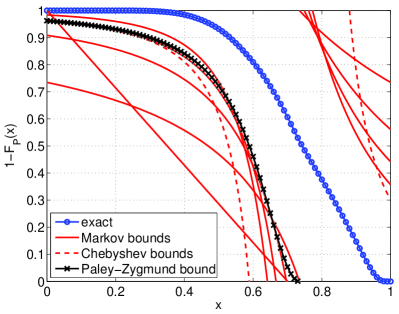
(a) $\lambda=1$, $p=1/4$, and $\operatorname{var}(P_{\rm s})=0.0212$.

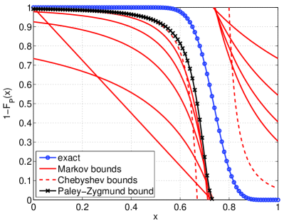
(b) $\lambda=5$, $p=1/20$, and $\operatorname{var}(P_{\rm s})=0.00418$

Figure 2: The exact meta distribution (11) and the Markov bounds (14) for $b\in[4]$, (15), and (16) for $\alpha=4$, $\theta=1$, $R=1/2$, and $\lambda p=1/4$. The resulting mean success probability is $p_{s}=M_{1}=0.735$. The variance depends on the values of $p$ and $\lambda$; it is proportional to $p$ for small $p$.

Corollary 4 (Markov and Chebyshev bounds)

For $x\in[0,1]$, the meta distribution is bounded as

$$1-\frac{\mathbb{E}^{!t}((1-P_{\rm s}(\theta))^{b})}{(1-x)^{b}}<\bar{F}(\theta,x)\leq\frac{M_{b}}{x^{b}},\quad b>0.$$ (14)

Let $V\triangleq\operatorname{var}P_{\rm s}(\theta)=M_{2}-M_{1}^{2}$. For $x<M_{1}$,

$$\bar{F}_{P_{\rm s}}(x)>1-\frac{V}{(x-M_{1})^{2}},$$ (15)

while for $x>M_{1}$,

$$\bar{F}_{P_{\rm s}}(x)\leq\frac{V}{(x-M_{1})^{2}}.$$ (16)

Lastly,

$$\bar{F}_{P_{\rm s}}(xM_{1})\geq\frac{(1-x)^{2}}{1-M_{1}^{p(1-\delta)}+(1-x)^{2}},\quad x\in(0,1).$$ (17)

Proof:

(14) follows from Markov’s inequality, while (15) and (16) follow from Chebyshev’s inequality. The lower bound (17) is the Paley-Zygmund (or Cauchy-Schwarz) bound. ∎

For the lower (or reverse) Markov bound in (14), the integer moments of $1-P_{\rm s}(\theta)$ are easily found using binomial expansion. For $b=-1$, the Markov inequality also yields the lower bound $\bar{F}_{P_{\rm s}}(x)\geq 1-xM_{-1}$, where $M_{-1}$ is given in (6).

These bounds are illustrated in the two plots in Fig. 2. For the Markov bounds, the four lower and upper bounds correspond to $b=1,2,3,4$. It is apparent that the variance decreases with decreasing $p$ and that the bounds get tighter also.

Written differently, (15) and (16) state that

$$\bar{F}_{P_{\rm s}}(qM_{1})>1-\frac{M_{1}^{\delta-1}-1}{(1-q)^{2}},\quad 0<q<1,$$

and

$$\bar{F}_{P_{\rm s}}(qM_{1})\leq\frac{M_{1}^{\delta-1}-1}{(1-q)^{2}},\quad 1<q<M_{1}^{-1}.$$

The upper bound is useful for small $M_{1}$, while the lower bound is useful for $M_{1}\approx 1$.

So as $p\to 0$, $\mathbb{P}(P_{\rm s}(\theta)\geq xM_{1})\to 1$ $\forall x\in(0,1)$, in accordance with Cor. 1.

The Paley-Zygmund bound is useful to bound the fraction of links that has at least a certain fraction of the average performance. For example, the fraction of links having better than half the average reliability is lower bounded as

$$\mathbb{P}^{!{\rm t}}(P_{\rm s}(\theta)\geq M_{1}/2)\geq\frac{1/4}{5/4-M_{1}^{p(1-\delta)}}.$$

As $p\to 0$, the lower bound approaches $1$, again as expected from the concentration result in Cor. 1.

II-E Best bounds given four moments

Here we establish the tightest possible lower and upper bounds on the distribution given the first four moments. Generally, this problem can be formulated as follows. Letting $\mathcal{M}_{k}$ be the class of distributions (cdfs) with moments $M_{1},\ldots,M_{k}$, we would like to find

$$L(x)\triangleq\min_{F\in\mathcal{M}_{k}}F(x),\quad x\in(0,1)$$

and

$$U(x)\triangleq\max_{F\in\mathcal{M}_{k}}F(x),\quad x\in(0,1).$$

So for each $x$ in the support of the distribution, we would like to find the minimum and maximum over all distributions with the prescribed $k$ moments. To find $L$ and $U$ for $k=4$, we are applying the method from [13]. It determines the best lower and upper bounds

$$L(x)\leq F_{Y}(x)\leq U(x)$$

given the four moments $\mathbb{E}(Y^{k})$, $k\in[4]$, for a general continuous random variable $Y$.

To bound the cdf $F_{Y}(x)$ at a target value $x$, first the moments are calculated for the random variable shifted by $x$ so that the new target location is $0$, i.e.,

$$m_{i}(x) \triangleq\int_{0}^{1}(y-x)^{i}\,\mathrm{d}F_{Y}(y)$$

$$=\sum_{k=0}^{i}\binom{i}{k}(-x)^{i-k}\mathbb{E}(Y^{k}),\quad x\in[0,1].$$

Using these shifted means, following [13], we define (omitting the dependence on $x$ of the shifted moments to avoid overly cumbrous notation)

$$q(x) \triangleq\sqrt{(-m_{2}m_{3}+m_{1}m_{4})^{2}-4(m_{2}^{2}-m_{1}m_{3})(m_{3}^{2}-m_{2}m_{4})}$$

$$p_{0}(x) \triangleq\frac{-m_{2}^{3}+2m_{1}m_{2}m_{3}-m_{3}^{2}-m_{1}^{2}m_{4}+m_{2}m_{4}}{m_{2}m_{4}-m_{3}^{2}}$$

$$y_{1}(x) \triangleq\frac{m_{2}m_{3}-m_{1}m_{4}-q(x)}{2(m_{2}^{2}-m_{1}m_{3})}$$

$$y_{2}(x) \triangleq\frac{m_{2}m_{3}-m_{1}m_{4}+q(x)}{2(m_{2}^{2}-m_{1}m_{3})}$$

$$p_{2}(x) \triangleq-\frac{m_{2}^{2}-m_{1}m_{3}}{q(x)}\left(-m_{1}-\frac{(m_{2}^{3}-2m_{1}m_{2}m_{3}+m_{1}^{2}m_{4})(-m_{2}m_{3}+m_{1}m_{4}+q(x)}{2(m_{2}^{2}-m_{1}m_{3})(-m_{3}^{2}+m_{2}m_{4})}\right)$$

$$p_{1}(x) \triangleq 1-p_{0}(x)-p_{2}(x),$$

and the bounds follow as

$$L(x)=\begin{cases}p_{1}(x)+p_{2}(x)&\text{if }y_{1}(x)<0,\>y_{2}(x)<0\\ p_{1}(x)&\text{if }y_{1}(x)<0,\>y_{2}(x)>0\\ 0&\text{if }y_{1}(x)>0,\>y_{2}(x)>0\end{cases}$$ (18)

$$U(x)=\begin{cases}1&\text{if }y_{1}(x)<0,\>y_{2}(x)<0\\ p_{0}(x)+p_{1}(x)&\text{if }y_{1}(x)<0,\>y_{2}(x)>0\\ p_{0}(x)&\text{if }y_{1}(x)>0,\>y_{2}(x)>0\end{cases}$$ (19)

Since $q(x)>0$, it is not possible that $y_{1}(x)>0$ and $y_{2}(x)<0$.

In our application $Y=P_{\rm s}(\theta)$, $\mathbb{E}(Y^{k})=M_{k}$, and since we are working with ccdfs, we have

$$1-U(x)\leq\bar{F}(\theta,x)\leq 1-L(x).$$

Fig. 3 shows these best bounds, together with the lower and upper envelopes of the Markov upper and lower bounds for $b\in[4]$ and the Paley-Zygmund lower bound. In some intervals, the classical bounds are near-optimum, while in others, the best bounds are significantly tighter.

The method in [13] is not restricted to four moments, but it is considerably more tedious to apply if more moments are considered.

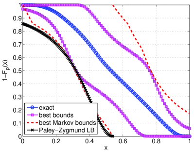
(a) $\lambda=1$ $\Rightarrow$ $p_{\rm s}=0.54$, $\operatorname{var}(P_{\rm s})=0.049$.

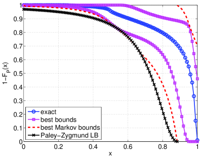
(b) $\lambda=1/5$ $\Rightarrow$ $p_{\rm s}=0.88$, $\operatorname{var}(P_{\rm s})=0.024$

Figure 3: The exact meta distribution (11), the best Markov bounds (14) for $b\in[4]$, and the best overall bounds per (18) and (19) (given the first four moments) for $\alpha=4$, $\theta=1$, $R=1/2$, and $p=1/2$. The reduction of $\lambda$ from $1$ to $1/5$ results in a reduction of the variance of only $1/2$, since $p$ stays the same.

II-F Approximation with beta distribution

Since $P_{\rm s}(\theta)$ is supported on $[0,1]$, a natural choice for a simple approximating distribution is the beta distribution. The probability density function (pdf) of a beta distributed random variable $X$ with mean $\mu$ is

$$f_{X}(x)=\frac{x^{\frac{\mu(\beta+1)-1}{1-\mu}}(1-x)^{\beta-1}}{{\rm B}(\mu\beta/(1-\mu),\beta)},$$

where ${\rm B}(\cdot,\cdot)$ is the beta function. The variance is given by

$$\sigma^{2}\triangleq\operatorname{var}X=\frac{\mu(1-\mu)^{2}}{\beta+1-\mu}.$$

Matching mean and variance $\sigma^{2}$ yields $\mu=M_{1}$ and

$$\beta=\frac{\mu(1-\mu)^{2}}{\sigma^{2}}-(1-\mu)=\frac{(\mu-M_{2})(1-\mu)}{M_{2}-\mu^{2}}.$$

As illustrated in Fig. 4 (same parameters as in Figs. 2 and 3), the beta distribution provides an excellent match for the distribution of the link success probabilities, which is also corroborated by the fact that the higher moments $\mathbb{E}(X^{k})$ of the matched beta distribution are very close to $M_{k}$. For example, for the parameters in Fig. 2(a), the analytical $-1$-st and $3$-rd through $8$-th moments differ by less than $3\%$, as shown in Table I. So the skewness and kurtosis and the mean local delay are approximated very accurately also.

	$k=-1$	$k=3$	$k=4$	$k=5$	$k=6$	$k=7$	$k=8$
$M_{k}$	1.4278	0.4418	0.3571	0.2947	0.2476	0.2110	0.1820
$\mathbb{E}(X^{k})$	1.4333	0.4412	0.3555	0.2921	0.2440	0.2066	0.1770
ratio	0.9962	1.0014	1.0044	1.0090	1.0147	1.0211	1.0280

TABLE I: Comparison of moments $M_{k}$ and $\mathbb{E}(X^{k})$ of the beta approximation for the parameter set in Fig. 2(a).

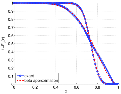
(a) Parameters from Fig. 2 (a) and (b).

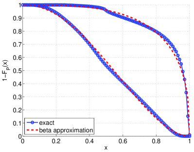
(b) Parameters from Fig. 3 (a) and (b).

Figure 4: The exact meta distribution and the beta distribution approximation for the two sets of parameters considered in the plots of Figs. 2 and 3.

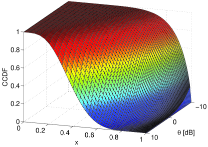
Figure 5: Three-dimensional plot of the meta distribution $\bar{F}(\theta,x)$ for $\lambda=1$, $p=1/4$, $\alpha=4$, and $R=1/2$.

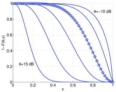
(a) Meta distribution for $\theta=-10,-5,0,5,10,15$ dB. The curve for $\theta=0$ dB is marked with $\circ$.

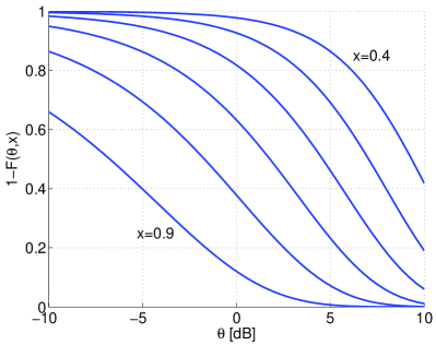
(b) Meta distribution as a function of $\theta$ for $x=0.4,0.5,0.6,0.7,0.8,0.9$.

Figure 6: Cross-sections through the meta distribution along the $x$ and $\theta$ axes for $\lambda=1$, $p=1/4$, $\alpha=4$, $R=1/2$.

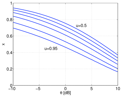
Figure 7: Contour plot of meta distribution $\bar{F}(\theta,x)$ for $\lambda=1$, $p=1/4$, $\alpha=4$, and $R=1/2$. The values at the curves are $\bar{F}(\theta,x)=u=0.5,0.6,0.7,0.8,0.9,0.95$ (from top to bottom).

II-G Illustrations of the meta distribution

An illustration of the meta distribution is shown in Fig. 5. It shows qualitatively that, for the chosen parameters, most links achieve an SIR of $-10$ dB with probability $80\%$, while an SIR of $10$ is achieved with probability $80\%$ by virtually no links. For quantitative purposes, the cross-sections and contours are more informative, as shown in the next figures.

Fig. 6(a) enables a more precise statement about the fraction of links achieving an SIR of $-10$ dB with $80\%$ reliability—it is $0.93$. It also shows that at $\theta=0$ dB, $60\%$ of the links have a success probability of at least $80\%$.

As a function of $\theta$ for fixed $x$, the value of $\theta$ can be determined such that at least a fraction $x$ of users have a success probability $p_{\rm min}$. For example, Fig. 6(b) shows that to achieve at least $80\%$ success probability for $80\%$ of the links, a $\theta$ of at most $-7.6$ dB can be chosen.

The contour plot Fig. 7 visualizes the trade-off between $x$ and $\theta$. It shows the combinations $(\theta,x)$ that can be achieved by a certain fraction of links $u$. For example, the curve for link fraction $u=0.95$ shows that $95\%$ of the links achieve an SIR of $-5$ dB with probability $0.6$ and an SIR of $5$ dB with probability $0.31$.

Hence the contour plot illustrates and quantifies the trade-off between data rate (as determined by $\theta$) and reliability (given by the parameter $x$) in bipolar networks.

III Poisson Cellular Networks

III-A System model

In Poisson cellular networks, base stations (BSs) form a PPP of intensity $\lambda$, while users form a stationary point process of intensity $\lambda_{\rm u}$. We focus on the downlink and on nearest-BS association, i.e., each BS serves all the users in its Voronoi cell, and first assume that all BSs are always active. An example realization where users form a square lattice is shown in Fig. 8.

As in the bipolar case, we assume the standard path loss law with path loss exponent $\alpha=2/\delta$ and Rayleigh fading. The standard (mean) success probability (or SIR distribution) is the success probability of the typical user, assumed at the origin $o$, which is known from [4] as

$$p_{\rm s}(\theta)=\mathbb{P}^{o}(\mathsf{SIR}>\theta)=\frac{1}{{}_{2}F_{1}(1,-\delta;1-\delta;-\theta)}.$$

The probability also has a spatial interpretation: for each realization of the BS and user point processes, it gives the fraction of users achieving an SIR of at least $\theta$ in a given time slot. It depends neither on the user density nor on the BS density.

Again we define the conditional success probability

$$P_{\rm s}(\theta)\triangleq\mathbb{P}^{o}(\mathsf{SIR}>\theta\mid\Phi),$$

which is the probability that the SIR at the origin exceeds $\theta$ given the BS process and given that a user is located at $o$. The quantity of interest is the meta distribution of the SIR, which is the distribution (ccdf) of $P_{\rm s}$:

$$\bar{F}(\theta,x)\triangleq\bar{F}_{P_{\rm s}}(x)=\mathbb{P}(P_{\rm s}(\theta)>x),\quad\theta\in\mathbb{R}^{+},\>x\in[0,1]$$

It gives detailed information about the user experience by providing the fraction of users achieving an SIR of $\theta$ with reliability at least $x$.

As before, a direct calculation of this meta distribution seems infeasible and we thus focus on the moments $M_{b}\triangleq\mathbb{E}(P_{\rm s}(\theta)^{b})$ first.

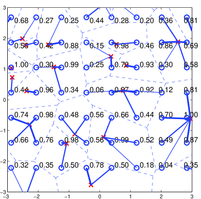
Figure 8: Realization of a Poisson cellular network with BS density $\lambda=1$, users forming a square lattice of density $\lambda_{\rm u}=3$, $\theta=1$, and $\alpha=4$, resulting in $p_{\rm s}=0.56$. The BSs are indicated by $\times$ and the users by $\circ$. The number next to each user is its success probability (averaged over fading) or its mark, and the dashed lines are the edges of the Voronoi cells of the BS PPP.

III-B Moments

Theorem 2 (Moments for cellular network)

The moments of the conditional success probability for Poisson cellular networks are given by

$$M_{b}=\frac{1}{{}_{2}F_{1}(b,-\delta;1-\delta;-\theta)},\quad b\in\mathbb{C}.$$ (20)

Proof:

Let $x_{0}=\operatornamewithlimits{arg\ min}\{x\in\Phi\colon\|x\|\}$ be the serving BS of the typical user. Given the BS process $\Phi$, the success probability is

$$P_{\rm s}(\theta) =\mathbb{P}\Big{(}h>\|x_{0}\|^{\alpha}\theta\sum_{x\in\Phi\setminus\{x_{0}\}}h_{x}\|x\|^{-\alpha}\>\Big{|}\>\Phi\Big{)}$$

$$=\prod_{x\in\Phi\setminus\{x_{0}\}}\frac{1}{1+\theta(\|x_{0}\|/\|x\|)^{\alpha}}.$$

The $b$-th moment follows as

$$M_{b}=\mathbb{E}\prod_{x\in\Phi\setminus\{x_{0}\}}\frac{1}{(1+\theta(\|x_{0}\|/\|x\|)^{\alpha})^{b}}.$$ (21)

Instead of calculating this expectation in two steps as usual (first condition on $\|x_{0}\|$ then take the expectation w.r.t. it), we use the recent result [14, Lemma 1], which requires the calculation of only one finite integral. The lemma gives the pgfl of the relative distance process (RDP), defined as

$$\mathcal{R}\triangleq\{x\in\Phi\setminus\{x_{0}\}\colon\|x_{0}\|/\|x\|\},$$

when $\Phi$ is a PPP. Since (21), depends on the BS locations only through the relative distances, we can directly apply the pgfl of the RDP and obtain

$$M_{b}=\frac{1}{1+2\int\limits_{0}^{1}\left(1-\frac{1}{(1+\theta r^{\alpha})^{b}}\right)r^{-3}\mathrm{d}r},$$ (22)

which can be expressed as (20). ∎

Sometimes the calculation of the hypergeometric function with negative last argument can cause numerical problems. In such cases, the alternative form

$$M_{b}=\frac{(1+\theta)^{b}}{{}_{2}F_{1}(b,1;1-\delta;\theta/(1+\theta))},$$

obtained through Euler’s transformation, is helpful.

For $b=-1$, (20) (or (22)—no “detour” using hypergeometric functions needed in this case) simplifies to

$$M_{-1}=\frac{1-\delta}{1-\delta(1+\theta)},\quad\theta<1/\delta-1.$$ (23)

As in the bipolar case, this is the mean local delay if $\theta<1/\delta-1$. Converseley, if $\theta\geq\alpha/2-1$, the mean local delay is infinite due to the correlated interference in the system. This phase transition in the mean local delay is similar to the one observed in [15, 11, 6] for ad hoc networks. Incidentally, the condition can also be expressed as $\theta\,\mathsf{MISR}<1$, where $\mathsf{MISR}$ is the mean interference-to-signal ratio of the PPP introduced in [16].

For $b\in\mathbb{N}$, the moment $M_{b}$ equals the joint success probability of $b$ transmissions, which was calculated in [7, Thm. 2] using a different (less direct) method.

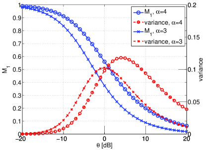
Figure 9: Success probability $M_{1}$ and variance $M_{2}-M_{1}^{2}$ for $\alpha=3$ and $\alpha=4$.

Fig. 9 shows the standard success probability $M_{1}=p_{\rm s}$ and the variance as a function of $\theta$ for $\alpha=3,4$. Since the variance necessarily tends to zero for both $\theta\to 0$ and $\theta\to\infty$, it assumes a maximum at some finite value of $\theta$. A numerical evaluation shows that for $\alpha=3$, the variance is maximized quite exactly at $\theta=1$, and for both values of $\alpha$, the success probability at which the variance is maximized is $p_{\rm s}=0.38$.

III-C Exact expression, bounds, and beta approximation

As in the bipolar case, we obtain an exact expression for the meta distribution from the Gil-Pelaez theorem.

Corollary 5

The SIR meta distribution for Poisson cellular networks is given by

$$\bar{F}(\theta,x)=\frac{1}{2}+\frac{1}{\pi}\int_{0}^{\infty}\frac{\Im(e^{-jt\log x}M_{jt})}{t}\mathrm{d}t$$ (24)

Numerical investigations indicate that $|M_{jt}|=\Theta(t^{-1})$, $t\to\infty$, so the integrand decays with $t^{-2}$ and the integral can be evaluated efficiently.

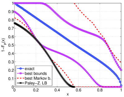
(a) $\theta=1$ $\Rightarrow$ $p_{\rm s}=0.56$, $\operatorname{var}(P_{\rm s})=0.098$

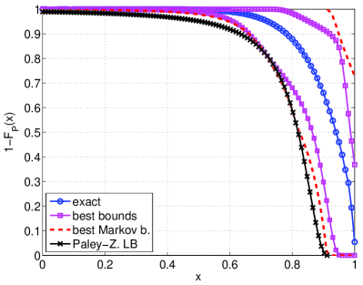
(b) $\theta=1/10$ $\Rightarrow$ $p_{\rm s}=0.91$, $\operatorname{var}(P_{\rm s})=0.0086$

Figure 10: The exact meta distribution (24), the best Markov bounds (14) for $b\in[4]$, the Paley-Zygmund lower bound, and the best overall bounds (given the first four moments) for $\alpha=4$.

Fig. 10 shows the exact distribution and the classical and best bounds for $\theta=1$ and $\theta=1/10$, respectively. Interestingly, the meta distribution $\bar{F}(1,x)$ has almost constant slope, which means that the user success probabilities are essentially uniformly distributed between $0$ and $1$.

Fig. 11 shows that the beta approximation provides an excellent fit over a wide range of $\theta$ values. It also serves as an illustration of the meta distribution showing what combinations of reliability $x$ and fraction of users can be achieved for $\theta\in\{-10,0,10\}$ dB.

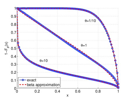
Figure 11: Exact ccdf and beta approximation for $\theta=1/10,1,10$ for $\alpha=4$.

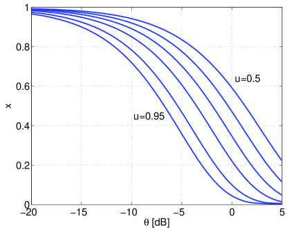
Figure 12: Contour plot of meta distribution $\bar{F}(\theta,x)$ for $\alpha=4$. The values at the curves are $\bar{F}(\theta,x)=u=0.5,0.6,0.7,0.8,0.9,0.95$ (from top to bottom).

Lastly, Fig. 12 shows a contour plot of the meta distribution for $\alpha=4$. An operator who is interested in the performance of the “5% user” (the user in the bottom 5-th percentile in terms of performance) can use the bottom curve, corresponding to $\bar{F}(\theta,x)=0.95$, to find the performance trade-off that such a user can achieve. For example, it can achieve an SIR of $-10$ dB with reliability $0.72$ or an SIR of $-4.3$ dB with reliability $0.3$.

III-D Effect of random base station activity

Here we investigate the effect on the meta distribution if interfering BSs were active only with probability $p$. This is similar to the model studied in [4, Sec. VI], where a frequency reuse parameter $\kappa$ was introduced and each BS is assumed to choose one of $\kappa$ bands independently at random. Hence the two models are the same if we set $p=\kappa^{-1}$ (apart from the fact that $\kappa\in\mathbb{N}$, whereas no such restriction is imposed on $p^{-1}$).

Theorem 3

The $b$-th moment of the success probability in a Poisson cellular network where interfering BSs are active independently with probability $p$ can be expressed as

$$M_{b}(p)=\left(1-\sum_{k=1}^{\infty}\binom{b}{k}(-p\theta)^{k}\frac{\delta}{k-\delta}\,_{2}F_{1}(k,k-\delta;k+1-\delta;-\theta)\right)^{-1}.$$ (25)

Proof:

If interfering BSs are active independently with probability $p$ in each time slot, we have

$$P_{\rm s}(\theta) =\prod_{r\in\mathcal{R}}\left(\frac{p}{1+\theta r^{\alpha}}+1-p\right)$$

and thus

$$M_{b}(p)=\mathbb{E}\prod_{r\in\mathcal{R}}\left(1-\frac{p\theta r^{\alpha}}{1+\theta r^{\alpha}}\right)^{b}.$$

Hence we need to modify (22) to

$$M_{b}(p)=\frac{1}{1+2\int\limits_{0}^{1}\Big{(}1-\left(1-\frac{p\theta r^{\alpha}}{1+\theta r^{\alpha}}\right)^{b}\Big{)}r^{-3}\mathrm{d}r}.$$ (26)

For general $b\in\mathbb{C}$, letting $x=r^{\alpha}$, the integral in (26) can be expanded as

$$\sum_{k=1}^{\infty}\binom{b}{k}\frac{-(-p\theta)^{k}}{\alpha}\int_{0}^{1}\left(\frac{x}{1+\theta x}\right)^{k}x^{-\delta-1}\mathrm{d}x=\\ \sum_{k=1}^{\infty}\binom{b}{k}\frac{-(-p\theta)^{k}}{k\alpha-2}\,_{2}F_{1}(k,k-\delta;k+1-\delta;-\theta),$$ (27)

and we obtain the result. ∎

For $b=1$, this yields the success probability

$$p_{\rm s}(\theta,p) =\frac{1}{1+p\theta\frac{\delta}{1-\delta}\,_{2}F_{1}(1,1-\delta;2-\delta,-\theta)}$$ (28)

$$=\frac{1}{1-p+p\,_{2}F_{1}(1,-\delta;1-\delta;-\theta)}$$ (29)

The first expression corresponds to [4, Eqn. (19)], while the second one follows from the identity

$$\frac{\theta\delta}{1-\delta}\ _{2}F_{1}(1,1-\delta;2-\delta;-\theta)+1\equiv\,_{2}F_{1}(1,-\delta;1-\delta;-\theta).$$ (30)

For $b=-1$, (26) yields

$$M_{-1}=\frac{1}{1-p\theta\frac{\delta}{1-\delta}\,_{2}F_{1}(1,1-\delta;2-\delta,-\theta(1-p))},\quad p\leq p_{\rm c}(\theta).$$ (31)

Here $p_{\rm c}(\theta)$ is the critical transmit probability denoting the phase transition from finite to infinite mean local delay. If $\theta<1/\delta-1$, we know from (23) that $p_{\rm c}(\theta)=1$. If $p<1$, a larger $\theta$ can be accommodated while maintaining a finite mean local delay. Fig. 13 shows the critical probability $p_{\rm c}(\theta)$ and two conjectured bounds, which are $p_{\rm c}(\theta)\geq(\frac{\delta}{1-\delta}\theta)^{-\delta}/2$ and $p_{\rm c}(\theta)\leq(\frac{\delta}{1-\delta}\theta)^{-\delta}$.

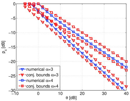
Figure 13: Critical probability $p_{\rm c}$ (in dB) for finite mean local delay as a function of $\theta$ for $\alpha=3,4$ and conjectured lower and upper bounds.

Next we provide an asymptotic result on the success probability $p_{\rm s}(p,\theta)$ as $p\to 0$ while keeping $p\theta^{\delta}$ constant.

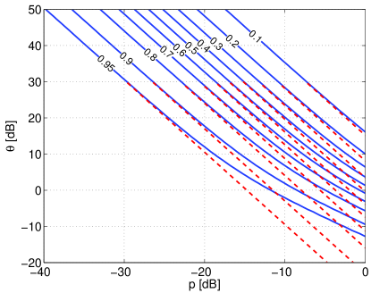
Figure 14: Contour plot showing the combinations of $\theta$ and $p$ (in dB) that achieve a given target success probability $p_{\rm t}\in\{0.1,0.2,\ldots,0.9,0.95\}$ for $\alpha=4$. The dashed lines are the asymptotes obtained from (32).

Corollary 6

Let $t=p\theta^{\delta}$. As $p\to 0$ and $\theta\to\infty$ such that $t$ stays constant,

$$p_{\rm s}(\theta,p)\sim\frac{1}{1+p\theta^{\delta}/\operatorname{sinc}\delta}=\frac{\operatorname{sinc}\delta}{t+\operatorname{sinc}\delta}.$$ (32)

Proof:

From Thm. 4 and Lemma 6 in [14], ${}_{2}F_{1}(1,-\delta;1-\delta;-\theta)\sim\theta^{\delta}/\operatorname{sinc}\delta$, $\theta\to\infty$. Inserting this in (29) and letting $p\to 0$ and $\theta\to\infty$ while keeping $p\theta^{\delta}$ constant yields the result. ∎

The corollary implies that

$$p_{\rm s}(\theta,p)\sim p_{\rm s}(c^{1/\delta}\theta,p/c),\quad c\geq 1.$$

So in the limit of small $p$, if $p$ is decreased by 10 dB, $\theta$ can be increased by $5\alpha$ dB to maintain the same success probability.

Fig. 14 shows a contour plot indicating the combinations of $\theta$ and $p$ (in dB) that achieve a given target success probability $p_{\rm t}$, together with the asymptotes obtained from (32) by calculating $t$ from $t=(p_{\rm t}^{-1}-1)\operatorname{sinc}\delta$ and then plotting $\theta(p)=(t/p)^{1/\delta}$, which is a line in the log-log plot. Hence, keeping $p\theta^{\delta}$ constant results asymptotically in the same success probability, as $p\to 0$ or $\theta\to\infty$; in contrast, in the bipolar case, keeping $p\theta^{\delta}$ constant results in exacty the same success probability for all values of $p$ and $\theta$.

An important question is whether—as in the bipolar case—the variance goes to $0$ as $p\to 0$ while keeping $p_{\rm s}$ constant. The last corollary answers that question.

Corollary 7

Given $t=p\theta^{\delta}$,

$$\lim_{\begin{subarray}{c}p\to 0\\ \theta=(t/p)^{1/\delta}\end{subarray}}\operatorname{var}P_{\rm s}(\theta,p)=\frac{\operatorname{sinc}\delta}{2t+\operatorname{sinc}\delta}-\left(\frac{\operatorname{sinc}\delta}{t+\operatorname{sinc}\delta}\right)^{2}.$$ (33)

Expressed as a function of the target success probability $p_{\rm t}$,

$$\lim_{\begin{subarray}{c}p\to 0\\ \theta=(t/p)^{1/\delta}\end{subarray}}\operatorname{var}P_{\rm s}(\theta,p)=\frac{p_{\rm t}}{2-p_{\rm t}}-p_{\rm t}^{2}.$$ (34)

Proof:

The inverse of the second moment follows from Thm. 3 and is given by

$$M_{2}^{-1}=1+2p\>\underbrace{\theta\frac{\delta}{1-\delta}\,_{2}F_{1}(1,1-\delta;2-\delta,-\theta)}_{A}-\>p^{2}\,\underbrace{\theta^{2}\frac{\delta}{2-\delta}\,_{2}F_{1}(2,2-\delta;3-\delta,-\theta)}_{B}.$$

As $\theta\to\infty$, combining (32) and (28), $A=\theta^{\delta}/\operatorname{sinc}\delta$. For $B$, we have $B=\Theta(\theta^{\delta})$. Hence, for some constant $c>0$,

$$\lim_{\begin{subarray}{c}p\to 0\\ \theta=(t/p)^{1/\delta}\end{subarray}}M_{2}^{-1}=1+2t/\operatorname{sinc}\delta-ptc=1+2t/\operatorname{sinc}\delta.$$

The result follows from $\operatorname{var}P_{\rm s}=M_{2}-M_{1}^{2}$, with $M_{1}$ given in (32). ∎

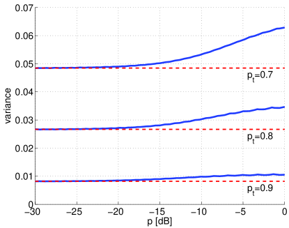
Figure 15: Variance $M_{2}-M_{1}^{2}$ as a function of the BS activity probability $p$ for target success probabilities $p_{\rm t}\in\{0.7,0.8,0.9\}$ for $\alpha=4$. The dashed lines are the asymptotes from (34).

Fig. 15 displays the variance as a function of $p$ for different target success probabilities. These are the variances obtained along the corresponding contour lines in Fig. 14. The asymptotic variance from (34) is also shown. It can be seen that the transmit probability has relatively little impact on the variance, especially for higher success probabilities. So, in contrast to the bipolar case, the disparity in the user experience cannot be significantly reduced by random BS activation patterns.

IV Conclusions

While spatial averages, such as the success probability of a transmission over the typical link (or standard SIR distribution), are useful, they do not provide much information about the performance of the individual links or users in a given realization of the network. To overcome this drawback, this paper introduces the meta distribution of the SIR, which is the distribution of the conditional SIR distribution (or success probability) given the point process, and provides an exact expression, bounds, and an approximation, for Poisson bipolar and cellular networks. Hence the complete distribution of the conditional link success probability $P_{\rm s}$ in both types of Poisson networks can be characterized. The complete distribution of $P_{\rm s}(\theta)$ provides much more fine-grained information that just the mean $p_{\rm s}(\theta)$ that is usually consiered.

The key insight is that the moments of $P_{\rm s}$ can be calculated in closed-form. Hence standard and optimum moment-based bounding techniques can be employed, which yield lower and upper bounds that are reasonably tight in some regimes. Moreover, an approximation by a beta distribution by matching first and second moments turns out to be matching the exact distributions extremely accurately.

Bipolar networks with ALOHA exhibit the interesting property that the variance of $P_{\rm s}$ goes to $0$ as the transmit probability $p\to 0$ while keeping the (mean) success probability constant. This is, however, not the case for cellular networks. If interfering base stations are active independently with probability $p$, the variance approaches a non-zero constant as $p\to 0$, again while keeping a constant success probability $p_{\rm s}$. So the deployment of an ultra-dense network of small cells that are only active with small probability (when a user requires service in their cell) does not significantly reduce the disparity of user experiences. On the positive side, lowering $p$ allows an increase of $\theta$ without affecting $p_{\rm s}$. To be precise, decreasing $p$ by 10 dB allows an increase of $\theta$ by $5\alpha$ dB.

From a broader perspective, the results show that it is possible in certain cases to not only derive spatial averages, but complete spatial distributions, which constitute rather sharp results on the network performance since they capture the statistics of all links in a given realization of the network. Hence it is demonstrated that stochastic geometry allows for the calculation of (even) stronger results than spatial averages.

References

- [1] F. Baccelli, B. Blaszczyszyn, and P. Mühlethaler, “An ALOHA Protocol for Multihop Mobile Wireless Networks,” IEEE Transactions on Information Theory, vol. 52, pp. 421–436, Feb. 2006.
- [2] M. Zorzi and S. Pupolin, “Optimum Transmission Ranges in Multihop Packet Radio Networks in the Presence of Fading,” IEEE Transactions on Communications, vol. 43, pp. 2201–2205, July 1995.
- [3] R. K. Ganti and J. G. Andrews, “Correlation of Link Outages in Low-Mobility Spatial Wireless Networks,” in 44th Asilomar Conference on Signals, Systems, and Computers (Asilomar’10), (Pacific Grove, CA), Nov. 2010.
- [4] J. G. Andrews, F. Baccelli, and R. K. Ganti, “A Tractable Approach to Coverage and Rate in Cellular Networks,” IEEE Transactions on Communications, vol. 59, pp. 3122–3134, Nov. 2011.
- [5] G. Nigam, P. Minero, and M. Haenggi, “Coordinated Multipoint Joint Transmission in Heterogeneous Networks,” IEEE Transactions on Communications, vol. 62, pp. 4134–4146, Nov. 2014.
- [6] M. Haenggi and R. Smarandache, “Diversity Polynomials for the Analysis of Temporal Correlations in Wireless Networks,” IEEE Transactions on Wireless Communications, vol. 12, pp. 5940–5951, Nov. 2013.
- [7] X. Zhang and M. Haenggi, “A Stochastic Geometry Analysis of Inter-cell Interference Coordination and Intra-cell Diversity,” IEEE Transactions on Wireless Communications, vol. 13, pp. 6655–6669, Dec. 2014.
- [8] M. Haenggi, Stochastic Geometry for Wireless Networks. Cambridge University Press, 2012.
- [9] M. Haenggi and R. K. Ganti, “Interference in Large Wireless Networks,” Foundations and Trends in Networking, vol. 3, no. 2, pp. 127–248, 2008. Available at http://www.nd.edu/~mhaenggi/pubs/now.pdf.
- [10] R. K. Ganti and M. Haenggi, “Spatial and Temporal Correlation of the Interference in ALOHA Ad Hoc Networks,” IEEE Communications Letters, vol. 13, pp. 631–633, Sept. 2009.
- [11] M. Haenggi, “The Local Delay in Poisson Networks,” IEEE Transactions on Information Theory, vol. 59, pp. 1788–1802, Mar. 2013.
- [12] J. Gil-Pelaez, “Note on the Inversion Theorem,” Biometrika, vol. 38, pp. 481–482, Dec. 1951.
- [13] S. Rázc, A. Tari, and M. Telek, “A moments based distribution bounding method,” Mathematical and Computer Modelling, vol. 43, pp. 1367–1382, June 2006.
- [14] R. K. Ganti and M. Haenggi, “Asymptotics and Approximation of the SIR Distribution in General Cellular Networks.” ArXiv, http://arxiv.org/abs/1505.02310, May 2015.
- [15] F. Baccelli and B. Blaszczyszyn, “A New Phase Transition for Local Delays in MANETs,” in IEEE INFOCOM’10, (San Diego, CA), Mar. 2010.
- [16] M. Haenggi, “The Mean Interference-to-Signal Ratio and its Key Role in Cellular and Amorphous Networks,” IEEE Wireless Communications Letters, vol. 3, pp. 597–600, Dec. 2014.