Quantum cellular automata without particles

Abstract

Quantum cellular automata (QCA) constitute space and time homogeneous discrete models for quantum field theories (QFTs). Although QFTs are defined without reference to particles, computations are done in terms of Feynman diagrams, which are explicitly interpreted in terms of interacting particles. Similarly, the easiest QCA to construct are quantum lattice gas automata (QLGA). A natural question then is, which QCA are not QLGA? Here we construct a non-trivial example of such a QCA; it provides a simple model in $1+1$ dimensions with no particle interpretation at the scale where the QCA dynamics are homogeneous.

I Introduction

The famous talk in which Feynman proposed the idea of quantum computers was entitled “Simulating physics with computers” Feynman (1982). In it he takes the point of view that to simulate physics on a computer, space and time should be discretized, and the dynamics should be local and causal; he comments that a natural architecture would be a cellular automaton. Since his goal is to simulate quantum physics, this would have to be a quantum cellular automaton (QCA). We may think of this as a discrete quantum field theory, discrete in space and time, but also with only a finite dimensional Hilbert space associated with each spacetime lattice site. Such a system should be able to simulate, for example, scattering of particles in $\phi^{4}$ quantum field theory, as has recently been shown to be possible with a quantum gate array architecture Jordan et al. (2012).

The investigation of QCA dates back to early papers of Grossing and Zeilinger Grossing and Zeilinger (1988), of Meyer Meyer (1996a, b), and of Durr and Santha Durr et al. (1997), some of which focused on the technically easier case of periodic boundary conditions. One of the main difficulties has always been to construct explicit models in which the conditions of translation invariance, unitarity, locality and causality are simultaneously satisfied. The easiest way forward has been to reinterpret translation invariance in order to allow quantum lattice gas automata (QLGA) models. We may note that studying (classical) lattice gas automata as a representative class within (classical) cellular automata (CA) has precedent in the works of Toffoli Toffoli et al. (2008) and Hénon Hénon (1988).

The more recent work, within the last decade, of Schumacher and Werner Schumacher and Werner (2004), Arrighi, et al. Arrighi et al. (2008), and of Shakeel and Love Shakeel and Love (2013) has developed frameworks within which more general models satisfying the requisite conditions can be constructed. Schumacher and Werner Schumacher and Werner (2004), and Gross, et al. Gross et al. (2012), have developed an axiomatic definition of QCA based on the desiderata of unitarity, locality and causality, as well as of translation invariance (spatial homogeneity) Schumacher and Werner (2004). In this formalism, the QCA dynamics are described on a quasi-local algebra, by which they mean an increasing chain of finitely many tensor products of finite dimensional $C^{*}$-algebras. The QCA evolution is in the Heisenberg picture, and given by an automorphism of quasi-local algebra by local rules Schumacher and Werner (2004); Gross et al. (2012). Within this setup, an index theory for a classification of one-dimensional QCA was developed in Gross et al. (2012). A parallel definition of one-dimensional QCA by Arrighi, et al. Arrighi et al. (2008) is given in the Schrödinger picture, i.e., one in which a QCA is defined on a Hilbert space and evolves unitarily. In this case the Hilbert space has as its basis finite but unbounded configurations (finitely many active cells in a quiescent background), and the QCA state in it evolves by a unitary, casual and translation-invariant global evolution operator. Shakeel and Love Shakeel and Love (2013), working in the latter formalism and building on it, found conditions that determine when a multi-dimensional QCA is a QLGA. They investigated QLGA because they are simple models for QCA and have obvious physical interpretations Meyer (1996a). Their characterization uses a different set of algebraic substructures than the ones used in the index theory in Gross et al. (2012), and is motivated by the goal of classification of multi-dimensional QCA explicitly by the form of the global evolution. They provide examples of QCA that are not QLGA, even in $1+1$ dimensions. These examples, however, do not propagate information, which leaves open the question of the existence of QCA in the Schrödinger picture model which have no particle interpretation, but which nevertheless propagate information. Analogously, the $\phi^{4}$ quantum field theory simulation result Jordan et al. (2012) leaves open the question of how efficient a simulation is possible in regimes or for initial conditions not interpretable as scattering particles.

Our goal here is to show by a simple $(1+1)$-dimensional construction in the Schrödinger picture that there are discrete quantum field theories (QCA) that propagate information, yet without particle interpretation (i.e., not QLGA) at the time scale where the QCA dynamics are homogeneous. In the Heisenberg picture, such examples are contained in the Clifford QCA presented in the work of Schlingemann, et al. Schlingemann et al. (2008). Ours is another step in the direction of classifying QCA by the dynamical processes at play in the transfer of information among cells. This is a program akin to that which has been carried out for reversible classical CA by Kari Kari (1999), Toffoli Toffoli (1977), and Toffoli and Margolus Toffoli and Margolus (1990).

This paper is organized as follows. Section II recalls the definition of QCA and QLGA, and the condition that determines when a QCA is a QLGA. Section III begins with the example that constitutes the main part of this paper: a one-dimensional QCA that cannot be described as a QLGA, although it is built by concatenating two QLGA. Analysis of this example leads us to a conjecture generalizing this method of constructing QCA to arbitrary lattice dimensions, cell Hilbert spaces and neighborhoods. Useful as this technique is, there are QCA that are not obtainable in this manner, as the last proposition of the section shows. Section IV is the conclusion with a summary of the results and a discussion of the wider context in which our work stands.

II Preliminaries

We consider the QCA model as formulated in Shakeel and Love (2013). In general, the lattice of cells is $\mathbb{Z}^{n}$. For the reader who is not specifically interested in the technical details encountered in defining Hilbert spaces and operators over infinite lattices, the lattice of cells can be taken as finite. This does not affect any of the interesting aspects of the example QCA we discuss. Wherever needed, we provide equivalent (and simpler) definitions for finite lattices, after the definitions for the infinite lattice. A finite lattice is of the form $\mathbb{Z}^{n}/(N_{1}\times\cdots\times N_{n})$ for some finite positive integers $N_{i}$, $1\leq i\leq n$, with the ends wrapping cyclically, or in other words, it is a torus. Unless we are exclusively considering the infinite lattice, in which case we will make that explicit, we denote a lattice by $\mathcal{L}$. Over each cell is an identical finite dimensional Hilbert space $W$. A cell has a finite neighborhood $\mathcal{E}=\{e_{1},e_{2},\ldots,e_{r}\}\subset\mathcal{L}$ of size $r$, which specifies the surrounding cells that influence its evolution. The neighborhood of cell $x\in\mathcal{L}$ is denoted by $\mathcal{E}_{x}=x+\mathcal{E}.$ Let $\mathcal{B}$ be an orthonormal basis of the cell Hilbert space $W$,

$$\mathcal{B}=\{\left|b\right\rangle\}.$$

For the infinite lattice $\mathcal{L}=\mathbb{Z}^{n}$, basis elements of the QCA Hilbert space are constructed as sequences consisting of a finite region of cells in active states immersed in a background of cells in a fixed (unit norm) quiescent state $\left|q\right\rangle\in W$. Hence this basis is called the finite configurations basis, denoted by $\mathcal{C}$,

$$\mathcal{C}=\bigg{\{} \bigotimes_{x\in\mathbb{Z}^{n}}\left|b^{x}\right\rangle:\left|b^{x}\right\rangle\in\mathcal{B},$$

$$\text{all but a finite number of }\left|b^{x}\right\rangle=\left|q\right\rangle\bigg{\}},$$ (1)

where $\left|b^{x}\right\rangle$ is the cell basis element at $x$. $\mathcal{C}$ is orthonormal with respect to the inner product induced on it from that on $W$. The QCA Hilbert space is the $\ell^{2}$-completion of $\mathcal{C}$, and is called the Hilbert space of finite configurations, denoted by $\mathcal{H}_{\mathcal{C}}$. This definition of the finite configurations basis ensures that it is countable, so that the Hilbert space of finite configurations is separable (in the topological sense). The naming convention given here is adopted from Arrighi et al. (2008); in the mathematics literature, this construction is called an incomplete infinite tensor product space, as in Guichardet (1972); von Neumann (1939).

For a finite lattice, we use the same terminology as for the infinite lattice, except the Hilbert space on which the QCA evolves, $\mathcal{H}_{\mathcal{C}}$, is the usual tensor product space,

$$\mathcal{H}_{\mathcal{C}}=\bigotimes_{x\in\mathcal{L}}W$$

with the basis $\mathcal{C}$ given by,

$$\mathcal{C}=\bigl{\{}\bigotimes_{x\in\mathcal{L}}\left|b^{x}\right\rangle:\left|b^{x}\right\rangle\in\mathcal{B}\}.$$

A QCA evolves by a unitary transformation on $\mathcal{H}_{\mathcal{C}}$, called the global evolution which we denote by $\mathcal{G}$. It is required to be

1. Translation invariant: A translation operator $\tau_{z}$, for some $z\in\mathcal{L}$, is defined by its action on an element $\bigotimes_{x\in\mathcal{L}}|b^{x}\rangle\in{\mathcal{C}}$:

   $$\tau_{z}:\bigotimes_{x\in\mathcal{L}}\left|b^{x}\right\rangle\mapsto\bigotimes_{x\in\mathcal{L}}\left|b^{x+z}\right\rangle$$

   $\mathcal{G}$ is translation invariant if $\tau^{\vphantom{-1}}_{z}\mathcal{G}\tau^{-1}_{z}=\mathcal{G}$ for all $z\in\mathcal{L}$. Note $\tau_{z}$ is unitary, i.e., $\tau^{-1}_{z}=\tau^{{\dagger}}_{z}$.

2. Causal relative to a neighborhood $\mathcal{E}$: $\mathcal{G}$ is causal relative to a neighborhood $\mathcal{E}$ if for every pair $\rho,\rho^{\prime}$, of density operators on ${\mathcal{H}}_{\mathcal{C}}$, and $x\in\mathcal{L}$, that satisfy:

   $$\rho|_{\mathcal{E}_{x}}=\rho^{\prime}|_{\mathcal{E}_{x}}\text{,}$$

   the operators $\mathcal{G}\rho\mathcal{G}^{\dagger},\mathcal{G}\rho^{\prime}\mathcal{G}^{\dagger}$ satisfy

   $$\mathcal{G}\rho\mathcal{G}^{\dagger}|_{x}=\mathcal{G}\rho^{\prime}\mathcal{G}^{\dagger}|_{x}$$

The state of a QCA is given by a density operator on ${\mathcal{H}}_{\mathcal{C}}$.

Remark 1

For the rest of the discussion, the neighborhood for a given QCA is the unique minimal set (under set inclusion) satisfying the causality condition above.

The concept of causality can equally well be discussed with respect to the evolution, under conjugation by $\mathcal{G}$, of operators local upon a finite number of cells, i.e., non-identity on those cells and identity on all other cells.

To define local operators for the infinite lattice, we first look at the Hilbert space ${\mathcal{H}}_{\mathcal{C}}$ as composed of a finite part and a countably infinite part.

Definition 2

Let $D\subset\mathbb{Z}^{n}$ be a finite subset. Define the set of co-$D$ configurations to be ${\mathcal{C}}_{\overline{D}}:=\{\bigotimes_{i\in\mathbb{Z}^{n}\setminus D}|{c}_{i}\rangle:{c}_{i}\in{Q},\text{ all but finite }|{c}_{i}\rangle=\left|q\right\rangle\}$. Let the inner product on ${\mathcal{C}}_{\overline{D}}$ be induced by the inner product on $W$  as in the case of ${\mathcal{C}}$. Then the co-$D$ space, denoted by $\mathcal{H}_{{\mathcal{C}}_{\overline{D}}}$, is defined as the completion of $\text{span}({\mathcal{C}}_{\overline{D}})$ under the induced $l^{2}$ norm.

To be able to refer to operators on a finite subset of tensor factors in the infinite lattice case, we simply embed $\bigotimes_{j\in D}\rm{End}(W)$ into a subalgebra of $B({\mathcal{H}}_{\mathcal{C}})$ (the algebra of bounded linear operators on $\mathcal{H}_{\mathcal{C}}$),

$$\iota_{D}:\bigotimes_{j\in D}\rm{End}(W) \hookrightarrow B({\mathcal{H}}_{\mathcal{C}})$$ (2)

$$a \mapsto a\otimes\mathbb{I}_{\overline{\mathcal{D}}}$$

where $a$ is an element of $\bigotimes_{j\in D}\rm{End}(W)$, and $\mathbb{I}_{\overline{\mathcal{D}}}$ is the identity operator on the co-$D$ space, $\mathcal{H}_{{\mathcal{C}}_{\overline{D}}}$. Through the embedding $\iota_{D}$ (2) the algebra $\bigotimes_{j\in D}\rm{End}(W)$ is isomorphic to the corresponding finite dimensional subalgebra of $B({\mathcal{H}}_{\mathcal{C}})$. Then, for the infinite lattice, we define local operators as follows.

Definition 3

A linear operator $M$ on ${\mathcal{H}}_{\mathcal{C}}$ is local upon a finite subset $D\in\mathbb{Z}^{n}$ if it is in the image of the map $\iota_{D}$ (2).

For a finite lattice, the operators local upon $D\subset\mathcal{L}$ are

$$\bigotimes_{j\in D}\rm{End}(W)\otimes\bigotimes_{j\in\mathcal{L}\setminus D}\mathbb{I},$$

where $\rm{End}(W)$ is the set of linear operators on $W$, and $\mathbb{I}$ is the identity operator on $W$.

The next theorem, relating causality to evolution of local algebras, will need the reflected neighborhood, denoted by $\mathcal{V}$,

$$\mathcal{V}=-\mathcal{E}$$

As with the neighborhood, the reflected neighborhood of cell $z$ is denoted by $\mathcal{V}_{z}=z+\mathcal{V}$.

The expression of causality in this picture is given by the structural reversibility theorem due to Arrighi, et al. in Arrighi et al. (2008). A proof of this theorem is in Shakeel and Love (2013).

Theorem 4 (Structural Reversibility)

Let $\mathcal{G}:\mathcal{H}_{\mathcal{C}}\longrightarrow\mathcal{H}_{\mathcal{C}}$ be a unitary operator and $\mathcal{E}$ a neighborhood. Then the following are equivalent.

1. $\mathcal{G}$ is causal relative to the neighborhood $\mathcal{E}$.

2. For every operator $A_{z}$ local upon cell $z$, $\mathcal{G}^{\dagger}A_{z}\mathcal{G}$ is local upon $\mathcal{E}_{z}$.

3. $\mathcal{G}^{\dagger}$ is causal relative to the reflected neighborhood $\mathcal{V}$.

4. For every operator $A_{z}$ local upon cell $z$, $\mathcal{G}A_{z}\mathcal{G}^{\dagger}$ is local upon ${\mathcal{V}}_{z}$.

A QLGA models particles propagating on a lattice and scattering by interaction at the lattice sites. Each cell can be occupied by multiple particles, and each particle has a state which is a vector in a subcell Hilbert space $W_{j}$. Let us say that the internal states of particle $j$, $1\leq j\leq d$, are elements of the subcell Hilbert space $W_{j}$, so the cell Hilbert space is $W=\bigotimes_{j=1}^{d}W_{j}$. The quiescent state needed for the infinite configurations basis for an infinite lattice as in Eq. (II), $\left|q\right\rangle\in\bigotimes_{j\in\mathcal{E}}W_{j}$, is a pure tensor, i.e., has the form

$$\left|q\right\rangle=\bigotimes_{j\in\mathcal{E}}\left|q_{j}\right\rangle$$

for some unit norm $\left|q_{j}\right\rangle\in W_{j}$.

The basis $\mathcal{B}$ of the cell Hilbert space $W$ is expressed in terms of some orthonormal bases $\mathcal{B}_{j}$ of $W_{j}$,

$$\mathcal{B}=\{\left|b\right\rangle=\bigotimes_{j=1}^{d}\left|b_{j}\right\rangle:\left|b_{j}\right\rangle\in\mathcal{B}_{j}\}.$$

In the propagation stage of the evolution, a particle with internal state $j$ (or equivalently, that occupies subcell state $j$) hops to the corresponding subcell $j$ of a designated neighboring cell that is $e_{j}\in\mathcal{L}$ away. Naturally, this requires the collection of such neighbors to be specified by the neighborhood $\mathcal{E}=\{e_{1},e_{2},\ldots,e_{d}\}\subset\mathcal{L}$, of cardinality $|\mathcal{E}|=d$. Thus the global evolution is described by two unitary steps,

1. Advection, $\sigma$, that shifts the appropriate subcell state to the corresponding neighbor,

   $$\left.\begin{array}[]{cccc}\sigma:\bigotimes_{x\in\mathcal{L}}\bigotimes_{j=1}^{d}\left|b^{x}_{j}\right\rangle\mapsto\bigotimes_{x\in\mathcal{L}}\bigotimes_{j=1}^{d}\left|b^{x+e_{j}}_{j}\right\rangle,\end{array}\right.$$ (3)

   where $\left|b^{x}_{j}\right\rangle\in\mathcal{B}_{j}$, and the cell index $x$ indexes the subcell bases elements $\left|b^{x}_{j}\right\rangle$.

2. Scattering, $\hat{S}$, which acts on each cell by a local unitary scattering map $S:W\longrightarrow W$,

   $$\hat{S}:\bigotimes_{x\in\mathcal{L}}\bigotimes_{j=1}^{d}\left|b^{x}_{j}\right\rangle\mapsto\bigotimes_{x\in\mathcal{L}}S(\bigotimes_{j=1}^{d}\left|b^{x}_{j}\right\rangle).$$ (4)

   Note that in the infinite lattice case, $S$ must fix the quiescent state, i.e., $S(\left|q\right\rangle)=\left|q\right\rangle$.

Each time step, the current state of the QLGA is mapped unitarily to the next by its global evolution $\mathcal{G}$,

$$\mathcal{G}=\hat{S}\sigma$$

The state of a QLGA is an element of $\mathcal{H}_{\mathcal{C}}$. It is clear that a QLGA is a QCA. We observe that the advection $\sigma$ in (i) is completely specified by the neighborhood $\mathcal{E}$. We denote a QLGA by a pair $(\sigma,S)$.

Let us describe the criterion from Shakeel and Love (2013) for a QCA to be a QLGA. Denote the image, under $\mathcal{G}$, of operators localized on a single cell by

$$\mathcal{G}_{z}=\mathcal{G}^{\dagger}\mathcal{A}_{z}\mathcal{G},$$

Let us further denote by $\mathcal{D}_{z,x}$ the following subalgebra of $\mathcal{G}_{z}$, $z\in\mathbb{Z}^{n}$.

$$\mathcal{D}_{z,x}=\mathcal{G}_{z}\cap\mathcal{A}_{x}$$

When $z\in\mathcal{V}_{x}$ then $\mathcal{D}_{z,x}$ are the elements of $\mathcal{G}_{z}$ which are contained in $\mathcal{A}_{x}$, where

$$\mathcal{G}_{z}=\mathcal{G}^{\dagger}\mathcal{A}_{z}\mathcal{G}\subset\bigotimes_{k\in\mathcal{E}_{z}}\rm{End}(W)$$

and

$$\mathcal{A}_{z}=\underbrace{\rm{End}(W)}_{k=z}\otimes\bigotimes_{k\in\mathcal{E}_{z}\setminus\{z\}}\mathbb{I}_{k}.$$

For a QCA to be QLGA, (by Corollary 6 below), it is necessary and sufficient that

$$\mathcal{A}_{y}=\rm{span}(\prod_{k\in\mathcal{E}}\mathcal{D}_{{y-k},y}),$$ (5)

for all $y\in\mathbb{Z}^{n}$.

Before proceeding to our construction in the next section, we give a summary of useful results from Shakeel and Love (2013), describing the embedding of patches $\mathcal{D}_{{x-y},x}$, originating from neighboring cells, into a cell algebra, when a QCA locally satisfies a QLGA condition.

Theorem 5

Suppose that $\mathcal{G}$ is the global evolution of a QCA with neighborhood $\mathcal{E}$. Then

$$\mathcal{A}_{x}=\rm{span}(\prod_{y\in\mathcal{E}}\mathcal{D}_{{x-y},x})$$

if and only if there exists an isomorphism of vector spaces,

$$T:W\longrightarrow\bigotimes_{j\in\mathcal{E}}W_{j}$$

for some vector spaces $\{W_{j}\}_{j\in\mathcal{E}}$. Under the isomorphism $T$, for each $y\in\mathcal{E}$,

$$\mathcal{D}_{{x-y},x}\cong\rm{End}(W_{y})\otimes\bigotimes_{j\in\mathcal{E},j\neq y}\mathbb{I}_{W_{j}}$$

The algebras $\mathcal{A}_{x}$ and $\mathcal{G}_{x}$ (the images of algebras $\mathcal{A}_{x}$ after one timestep of the global evolution $\mathcal{G}$) are very simply related to the patches $\mathcal{D}_{{x-y},x}$ under the conditions of the above theorem.

Corollary 6

Suppose that $\mathcal{G}$ is the global evolution of a QCA with neighborhood $\mathcal{E}$, and satisfies $\mathcal{A}_{x}=\rm{span}(\prod_{y\in\mathcal{E}}\mathcal{D}_{{x-y},x})$. Then

1. $\mathcal{A}_{x}=\rm{End}(W)\cong\bigotimes_{j\in\mathcal{E}}\rm{End}(W_{j})$, for all $x\in\mathbb{Z}^{n}$.

2. The dimension of $W$, $d_{W}$, is a product of the dimensions of $W_{j}$, $d_{W_{j}}$, i.e., $d_{W}=\prod_{j\in\mathcal{E}}d_{W_{j}}$.

3. $\mathcal{G}_{x}=\rm{span}(\prod_{k\in\mathcal{E}}\mathcal{D}_{x,{x+k}})\cong\bigotimes_{k\in\mathcal{E}}\rm{End}(W_{k})$.

For completeness, we also include the structure theorem that globally characterizes a QCA as a QLGA.

Theorem 7

$\mathcal{G}$ is the global evolution of a QCA on the Hilbert space of finite configurations $\mathcal{H}_{\mathcal{C}}$, with neighborhood $\mathcal{E}$, and satisfies $\mathcal{A}_{x}=\rm{span}(\prod_{y\in\mathcal{E}}\mathcal{D}_{{x-y},x})$, if and only if

1. there exists an isomorphism of vector spaces $T$,

   $$T:W\longrightarrow\bigotimes_{j\in\mathcal{E}}W_{j}$$

   for some vector spaces $\{W_{j}\}_{j\in\mathcal{E}}$. Under the isomorphism $T$, for each $y\in\mathcal{E}$,

   $$\mathcal{D}_{{x-y},x}\cong\rm{End}(W_{y})\otimes\bigotimes_{j\in\mathcal{E},j\neq y}\mathbb{I}_{W_{j}}$$

   Furthermore, $\hat{W}=\bigotimes_{j\in\mathcal{E}}W_{j}$ can be given an inner product such that $T$ is an inner product preserving isomorphism of Hilbert spaces.

2. $\mathcal{G}$ is given by

   $$\mathcal{G}\cong{\hat{S}}\sigma,$$

   where $\sigma$ is as in (3), and $\hat{S}$ is as in (4) in terms of a unitary map $S$ on $\bigotimes_{j\in\mathcal{E}}W_{j}$.

3. (For infinite lattice) $\left|\tilde{q}\right\rangle=T(\left|q\right\rangle)$ is a pure tensor, i.e., $\left|\tilde{q}\right\rangle=\bigotimes_{j\in\mathcal{E}}\left|\tilde{q}_{j}\right\rangle$ for some unit norm $\left|\tilde{q}_{j}\right\rangle\in W_{j}$, and $S$ in the definition of $\hat{S}$ fixes $\left|\tilde{q}\right\rangle$: $S\left|\tilde{q}\right\rangle=\left|\tilde{q}\right\rangle$.

III A class of QCA that are not QLGA

We illustrate, with a simple example, a class of QCA without particles. This QCA is composed of two QLGA, and is shown in Fig. 1.

Figure 1: A QCA which is not a QLGA

The global evolution is

$$\mathcal{G}=\hat{S}_{2}\sigma_{2}\hat{S}_{1}\sigma_{1}.$$ (6)

Here, assume $W_{1}=W_{2}=\mathbb{C}^{2}$, $\sigma_{1}$ is described by the neighborhood $\mathcal{E}_{1}=\{e_{1}=0,e_{2}=-1\}$ and $\sigma_{2}$ by the neighborhood $\mathcal{E}_{2}=\{e_{1}=+1,e_{2}=0\}$. For the infinite lattice case, we take the quiescent state to be $\left|q\right\rangle=\left|00\right\rangle$.

When either $S_{1}$ or $S_{2}$ is identity, this describes a QLGA. Indeed, if $S_{1}=\mathbb{I}$,

$$\mathcal{G}=\hat{S}_{2}\sigma_{2}\sigma_{1}.$$

For the composite advection $\sigma_{2}\sigma_{1}$, the neighborhood is $\mathcal{E}=\{e_{1}=+1,e_{2}=-1\}$. If $S_{2}=\mathbb{I}$,

$$\mathcal{G}=\sigma_{2}\hat{S}_{1}\sigma_{1}.$$ (7)

Observe that under the unitary isomorphism $\sigma^{-1}_{2}$ of $\mathcal{H}_{\mathcal{C}}$,

$$\sigma^{-1}_{2}:\mathcal{H}_{\mathcal{C}}\longrightarrow\mathcal{H}_{\mathcal{C}},$$ (8)

we can write the global evolution as

$$\tilde{\mathcal{G}}=\sigma^{-1}_{2}\mathcal{G}\sigma^{\vphantom{-1}}_{2}=\hat{S}^{\vphantom{-1}}_{1}\sigma^{\vphantom{-1}}_{1}\sigma^{\vphantom{-1}}_{2}.$$

This shows that $\mathcal{G}$ is equivalent to a QLGA.

We can describe this in a more intuitive way, by writing the global evolution in (7) as

$$\mathcal{G}=\sigma^{\vphantom{-1}}_{2}\hat{S}^{\vphantom{-1}}_{1}\sigma^{-1}_{2}\sigma^{\vphantom{-1}}_{2}\sigma^{\vphantom{-1}}_{1}.$$

The natural way to deal with this is to adjust the cell definition to accommodate the new scattering $\sigma^{\vphantom{-1}}_{2}\hat{S}^{\vphantom{-1}}_{1}\sigma^{-1}_{2}$. Using the tensor factor indexing as for the “standard” cell, we can make the scattering local by redefining a new cell as the grouping of tensor factors from adjacent standard cells as follows. The cell at position $y$ is

$$W_{1}^{y-1}\otimes W_{2}^{y}.$$ (9)

This new constructed cell is shown in Fig. 2, by shading the corresponding subcells in a matched way. Under this cell definition, the neighborhood for $\sigma_{2}\sigma_{1}$ is $\mathcal{E}=\{e_{1}=+1,e_{2}=-1\}$.

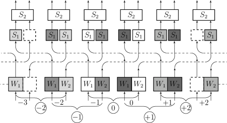
Figure 2: QCA of Fig. 1 as written in Eq. (11). The “regular” cell numbers are shown without circles under each qubit pair. Also the cells constructed as in Eq. (9) are shown as split across the regular cells, and their qubits shaded in a matched way, labeled by circled numbers. $\sigma_{2}\hat{S}_{1}\sigma^{-1}_{2}$ is depicted as pairs of smaller $S_{1}$ squares shaded corresponding to the new cell construction, where each pair of the same shade is a single $S_{1}$.

We define the construction of a new cell in a more general fashion. A cell can either be of the same size or an integer multiple of the size of the standard cell; this is dictated by the requirement that the evolution stay translation invariant. A new cell of the same size as the standard can only be defined through an advection as in the example above in (9); a set of such new cells can be grouped to obtain a larger cell.

Definition 8

Given a (current) cell Hilbert space $W=\bigotimes_{j=1}^{d}W_{j}$ and a set of finite configurations $\mathcal{C}$, a (new) cell construction is given by a neighborhood $\mathcal{E}_{c}=\{c_{1},\ldots,c_{d}\}\subset\mathbb{Z}^{n}$ (or equivalently an advection $\sigma_{c}$ corresponding to $\mathcal{E}_{c}$) and a positive integer $m$. Let us represent the current cell $x$ as a collection of pairs of indices

$$\{(x,j)\}_{j=1}^{d},$$

where $x$ is the cell index and $j$ is the subcell index. The new single cell $x$ is obtained by advection to get

$$\{(x+c_{j},j)\}_{j=1}^{d}.$$

A new larger cell $y$ is obtained by grouping $m$ such cells

$$\bigg{\{}(my+c_{j},j),\ldots,\bigl{(}m(y+1)-1+c_{j},j\bigr{)}\bigg{\}}_{j=1}^{d}.$$

In the subcell terminology, the constructed cell is

$$\bigotimes_{x=my}^{m(y+1)-1}\bigotimes_{j=1}^{d}W^{x+c_{j}}_{j}.$$ (10)

We note that in (8), $\sigma_{c}=\sigma^{-1}_{2}$ and $m=1$.

Next consider the case when neither $S_{1}$ nor $S_{2}$ is identity. We can write

$$\mathcal{G}=\hat{S}^{\vphantom{-1}}_{2}\sigma^{\vphantom{-1}}_{2}\hat{S}^{\vphantom{-1}}_{1}\sigma^{-1}_{2}\sigma^{\vphantom{-1}}_{2}\sigma^{\vphantom{-1}}_{1}.$$ (11)

This form of evolution is displayed in Fig. 2. $S_{1}$, which now shows up as $\sigma^{\vphantom{-1}}_{2}\hat{S}^{\vphantom{-1}}_{1}\sigma^{-1}_{2}$, is “spread out” by $\sigma_{2}$ over adjacent standard cells. However, there is no guarantee that the “scattering,”

$$\hat{S}^{\vphantom{-1}}_{2}\sigma^{\vphantom{-1}}_{2}\hat{S}^{\vphantom{-1}}_{1}\sigma^{-1}_{2},$$

is locally describable. That is, given a pair $S_{1},S_{2}$, one cannot always construct a cell such that $\mathcal{G}$ above can be written as a QLGA.

Theorem 9

For the QCA given by (6), there exist $S_{1}$ and $S_{2}$ such that the global evolution $\mathcal{G}$ in Eq. (6) is not equivalent to a QLGA for any cell construction.

Proof. Let us first rule out the cell configurations that worked in the two cases above. For the standard cell configuration (the one that worked for $S_{1}=\mathbb{I}$), a choice of $S_{1}$ and $S_{2}$ can be made to make the neighborhood $\mathcal{E}=\{e_{1}=-1,e_{2}=0,e_{3}=+1\}$. For instance, we can take $S_{1}=S_{2}=S$, the symmetric scattering matrix,

$$S=\begin{pmatrix}1&0&0&0\\ 0&1/\sqrt{2}&i/\sqrt{2}&0\\ 0&i/\sqrt{2}&1/\sqrt{2}&0\\ 0&0&0&i\\ \end{pmatrix}.$$ (12)

By the criterion in Shakeel and Love (2013) [Corollary 6 (ii)], the cell Hilbert space dimension, in this case $4$, must have $\left\lvert\mathcal{E}\right\rvert=r=3$ factors to be a QLGA. This condition is clearly not met. For the case of the cell configuration $W_{1}^{y-1}\otimes W_{2}^{y}$ (the one that worked when $S_{2}=\mathbb{I}$), the neighborhood is strictly $\mathcal{E}=\{e_{1}=-2,e_{2}=-1,e_{3}=+1,e_{4}=+2\}$, yielding $\left\lvert\mathcal{E}\right\rvert=r=4$. This runs into the same problem as before, as the cell Hilbert space dimension is again $4$. Hence these cell configurations cannot correspond to QLGA. In fact any cell construction based on single-cell ($m=1$) has this problem.

Next we consider more general cell constructions for this example. Take the cell to be $m\geq 2$ standard adjacent cells (the one that works for $S_{1}=\mathbb{I}$). Then the neighborhood is $\mathcal{E}=\{e_{1}=-1,e_{2}=0,e_{3}=+1\}$. $\left\lvert\mathcal{E}\right\rvert=r=3$, and the cell Hilbert space dimension is $2^{2m}$, so this is in agreement with Corollary 6 (ii). We need to resort to the criterion in Eq. (5) to show that the assertion still holds. Notice that $S$ in Eq. (12) has the property that, for $A,B,C\in M_{2}(\mathbb{C})$ (the algebra of $2\times 2$ complex matrices),

$$S^{\dagger}(\mathbb{I}\otimes A)S=B\otimes C\iff A=B=C=\mathbb{I}.$$ (13)

By the symmetry of $S$, this is also true if $\mathbb{I}\otimes A$ is replaced by $A\otimes\mathbb{I}$ in the above equation.

In the following, the subscripts and superscripts in the tensor factor indexing are as in Eq. (10). The property above implies, that up to conjugation by the local unitary $\bigotimes^{m}S_{2}=\bigotimes^{m}S$ (local relative to cells, i.e., acting by a cell-wise product of unitary transformations), we have that

$$\mathcal{D}_{{y-1},y} = \bigotimes_{x=my}^{m(y+1)-1}\bigotimes_{j=1}^{2}\mathbb{I}^{x}_{j},$$

$$\mathcal{D}_{{y},y} = \phantom{m}M_{2}(\mathbb{C})^{my}_{1}\otimes\mathbb{I}^{my}_{2}\otimes\bigg{(}\bigotimes_{x=my+1}^{m(y+1)-2}\bigotimes_{j=1}^{2}M_{2}(\mathbb{C})^{x}_{j}\bigg{)}$$

$$\phantom{m}\otimes\mathbb{I}^{m(y+1)-1}_{1}\otimes M_{2}(\mathbb{C})^{m(y+1)-1}_{2},$$

$$\mathcal{D}_{{y+1},y} = \bigotimes_{x=my}^{m(y+1)-1}\bigotimes_{j=1}^{2}\mathbb{I}^{x}_{j}.$$

This implies

$$\mathcal{A}_{y}\supsetneq\rm{span}(\prod_{k\in\mathcal{E}}\mathcal{D}_{{y-k},y}).$$ (15)

Thus this cell structure is not compatible with a QLGA.

Remark 10

To attain (15), the hypothesis on $S$ (when $S_{1}=S_{2}=S$) is weaker than the property in (13). Even so, the authors think $S\in M_{2}(\mathbb{C})$ satisfying  (13) are generic.

Observe from Eq. (III) that for $m>2$ the same considerations as $m=2$ apply when the criterion in Eq. (5) is used. Knowing this, we consider the cell structure in Eq. (9) and show how a grouping of two such cells, i.e., $m=2$, is incompatible with a QLGA when $S_{1}=S_{2}=S$. The new ($m=2$) cell $0$, for example, is formed by the single cells circled $0$ and $+1$ in Fig. 2. When we refer to cell $y$, we implicitly view this larger cell $0$ as the prototype. That said, cell $y$ is

$$(W^{2y-1}_{1}\otimes W^{2y}_{2})\otimes(W^{2y}_{1}\otimes W^{2y+1}_{2}),\\$$

and the same applies to the neighbors, where the neighborhood is (in units of this larger cell) $\mathcal{E}=\{e_{1}=-1,e_{2}=0,e_{3}=+1\}$. We begin by looking at $\mathcal{D}_{{y+1},y}$. We would like to show that

$$\text{dim }\mathcal{D}_{{y+1},y}<\text{dim }M_{2}(\mathbb{C})=4.$$ (16)

This involves a diagram chase. First, we see that the only influence on cell $y$ from cell $y+1$ is from the tensor factors in the following set with the arrows showing their endpoints after advection but before the action of respective $S_{1}$’s,

$$W^{2y+1}_{1} \mapsto W^{2y}_{1},$$

$$W^{2y+2}_{1} \mapsto W^{2y+1}_{1}.$$

Therefore, we start with an operator which is a finite sum of elements of the form (we include only the identity factors that matter)

$$(a^{2y}_{1}\otimes\mathbb{I}^{2y}_{2})\otimes(b^{2y+1}_{1}\otimes\mathbb{I}^{2y+1}_{2})\otimes(\mathbb{I}^{2y+2}_{1}\otimes\mathbb{I}^{2y+2}_{2}),$$ (18)

where $a^{2y}_{1},b^{2y+1}_{1}\in M_{2}(\mathbb{C})$. This sum is acted on by the relevant $S_{1}$’s to give a finite sum of elements of the form

$$\mathbb{I}^{2y}_{2}\otimes S_{1}^{\dagger}(a^{2y}_{1}\otimes\mathbb{I}^{2y+1}_{2})S_{1}\otimes S_{1}^{\dagger}(b^{2y+1}_{1}\otimes\mathbb{I}^{2y+2}_{2})S_{1}\otimes\mathbb{I}^{2y+2}_{1},$$ (19)

where we have exhibited the indices that are acted on by the $S_{1}$’s. Since $\mathcal{D}_{{y+1},y}$ is non-identity only on cell $y$, we see that after the action of $S_{2}$’s on the above, we get a finite sum of elements of the form

$$(g^{2y}_{1}\otimes h^{2y}_{2})\otimes(\mathbb{I}^{2y+1}_{1}\otimes s^{2y+1}_{2})\otimes(\mathbb{I}^{2y+2}_{1}\otimes\mathbb{I}^{2y+2}_{2}).$$ (20)

We observe that $S_{2}=S$, and that conjugation by local (in this case $S_{2}$ action on pairs of qubits) unitary operators cannot change an “entangled” (not a product) operator to an “unentangled” operator (a product). This implies in particular that after the conjugation action of $S_{1}$’s (before the action of $S_{2}$’s), the elements in (19) are of the form

$$(t^{2y}_{1}\otimes\mathbb{I}^{2y}_{2})\otimes(\mathbb{I}^{2y+1}_{1}\otimes p^{2y+1}_{2})\otimes(\mathbb{I}^{2y+2}_{1}\otimes\mathbb{I}^{2y+2}_{2}).$$

This further implies that the original element (18) must be of the form

$$(a^{2y}_{1}\otimes\mathbb{I}^{2y}_{2})\otimes(\mathbb{I}^{2y+1}_{1}\otimes\mathbb{I}^{2y+1}_{2})\otimes(\mathbb{I}^{2y+2}_{1}\otimes\mathbb{I}^{2y+2}_{2}).$$ (21)

To show (16), we need to find an element of the form (21) whose image after the action of $S_{1}$’s and $S_{2}$’s is not of the form (20). These elements abound. For instance, using

$$a^{2y}_{1}=\begin{pmatrix}1&0\\ 0&0\\ \end{pmatrix}.$$

in (21) works. This shows that

$$\text{dim }\mathcal{D}_{{y+1},y}<\text{dim }M_{2}(\mathbb{C})=4.$$

By symmetry,

$$\text{dim }\mathcal{D}_{{y-1},y}<\text{dim }M_{2}(\mathbb{C})=4.$$

Such reasoning in the context of $\mathcal{D}_{{y},y}$ also shows that

$$\text{dim }\mathcal{D}_{{y},y}=\bigl{(}\text{dim }M_{2}(\mathbb{C})\bigr{)}^{2}=16.$$

Combined, these imply

$$\text{dim }\mathcal{A}_{y}>\text{dim }\rm{span}(\prod_{k\in\mathcal{E}}\mathcal{D}_{{y-k},y}).$$

Thus this cell structure is also not compatible with a QLGA. It is clear that any other cell constructions that are based on single cells other than the ones just considered, i.e., constructed through other advection operators, can be similarly shown to be incompatible with a QLGA description. For $m>2$ the argument follows the same steps. Hence this shows that there is a pair of $S_{1}$, $S_{2}$ such that the QCA given in (11) and Fig. 1 is not a QLGA for any cell construction.   

We call a neighborhood, hence a QCA, trivial, if there is only one element in the neighborhood. When concerned with a QLGA, in which the neighborhood determines the advection, we also refer to the advection as trivial when the neighborhood is trivial, i.e., $\mathcal{E}=\{e_{1}=\cdots=e_{d}\}$ (here $d$ is the number of tensor factors of the cell Hilbert space $W=\bigotimes_{j=1}^{d}W_{j}$).

Generalizing the above result, we state the following.

Conjecture 11

Suppose $\mathcal{H}_{\mathcal{C}}$ is a Hilbert space of finite configurations with the cell Hilbert space $W=\bigotimes_{j=1}^{d}W_{j}$. Let $\sigma_{1}$ and $\sigma_{2}$ be two non-trivial advection operators on $\mathcal{H}_{\mathcal{C}}$. Then there exist unitary transformations $S_{1}$ and $S_{2}$ on $W$, such that the QCA formed by concatenating the QLGA $(\sigma_{1},S_{1})$ and $(\sigma_{2},S_{2})$, i.e., given by the global evolution $\mathcal{G}$,

$$\mathcal{G}=\hat{S}_{2}\sigma_{2}\hat{S}_{1}\sigma_{1},$$

is not equivalent to a QLGA for any cell construction.

One might imagine that such constructions can yield the most general QCA. Such is not the case as shown by the following.

Proposition 12

There exist finite length QCA that are not equivalent to a concatenation of finitely many QLGA.

Proof. If a QCA with cell Hilbert space of prime dimension is a concatenation of QLGA, then the constituent QLGA must have cell Hilbert spaces of prime dimension (the same as the QCA). Since every QLGA with cell Hilbert space of prime dimension is trivial, and trivial QLGA when concatenated can only yield a trivial QCA, this implies that the original QCA must be trivial. But there exist non-trivial finite length QCA on qubits, for example some Clifford QCA (CQCA) Schlingemann et al. (2008), in particular the CQCA of example $1.1$ in Schlingemann et al. (2008) (such non-trivial CQCA are more generally defined in Schlingemann et al. (2008) for other prime dimensions as well).   

Remark 13

In Schlingemann et al. (2008), the QCA definition is in the Heisenberg or operator picture. Since we are interested in unitary evolution, or the Schrödinger picture, we may only cite finite length versions of the CQCA, namely those for which the global evolution operator always exists.

This result indicates that there are interpretations of QCA beyond the regime of QLGA and concatenated constructions. The proof that we have given of the above proposition is valid only for finite length QCA. To the authors’ knowledge, this proposition is unproven for infinite length QCA as defined in this paper in the Schrödinger picture.

IV Conclusion

In this paper, we constructed a QCA, on a one-dimensional lattice, from a concatenation of two simple QLGA such that the constructed QCA is itself not a QLGA. In other words this QCA has no particle interpretation at the time scale at which the QCA dynamics are homogeneous. The proof of its non-QLGA behavior relies on application of the condition developed in Shakeel and Love (2013) characterizing when a QCA is a QLGA. In the same paper, it was noted that the question of complete QCA classification is still open. We hope this construction is a step in the process of answering that question. Our analysis suggests the conjecture that a more general result is possible, in which arbitrary cell dimension, lattice dimension, and any neighborhood scheme (except the trivial neighborhood) can be used in constructing such QCA from QLGA. For finite length QCA, we showed by citing the Clifford QCA in Schlingemann et al. (2008), that not all QCA can be expressed as concatenations of finitely many QLGA. In the larger theme of quantum simulations, and in view of the important work of Jordan, et al. Jordan et al. (2012) on simulation of $\phi^{4}$ quantum field theory, the question arises as to the efficiency with which a quantum simulation model might simulate physics without a particle description.