Level Crossings
in a
PT-symmetric Double Well

Abstract
We consider a PT-symmetric cubic oscillator with an imaginary double well. We prove the existence of an infinite number of level crossings with a definite selection rule. Decreasing the positive parameter $\hbar$ from large values, at a parameter $\hbar_{n}$ we find the crossing of the pair of levels $(E_{2n+1}(\hbar),E_{2n}(\hbar))$ becoming the pair of levels $(E_{n}^{+}(\hbar),E_{n}^{-}(\hbar))$. For large parameters, a level is a holomorphic function $E_{m}(\hbar)$ with different semiclassical behaviors, $E_{j}^{\pm}(\hbar),$ along different paths. The corresponding $m$-nodes delocalized state $\psi_{m}(\hbar)$ behaves along the same paths as the semiclassical $j$-nodes states $\psi_{j}^{\pm}(\hbar),$ localized at one of the wells $x_{\pm}$ respectively. In particular, if the crossing parameter $\hbar_{n}$ is by-passed from above, the levels $E_{2n+(1/2)\pm(1/2)}(\hbar)$ have respectively the semiclassical behaviors of the levels $E_{n}^{\mp}(\hbar)$ along the real axis. These results are obtained by the control of the nodes. There is evidence that the parameters $\hbar_{n}$ accumulate at zero and the accumulation point of the corresponding energies is an instability point of a subset of the Stokes complex called the monochord, consisting of the vibrating string and the sound board.

1 Introduction

The anharmonic oscillators are among the simplest non solvable models in quantum mechanics. In addition to presenting some connections with quantum field theory, their main interest mainly lies in the presence of diverging perturbation series and in the problem of their summability [1]. The latter is related to the existence of singularities of the levels as functions of the perturbation parameter. Since the family of Hamiltonians is analytic [2], such singularities are due to level crossings. The semiclassical theory provides good qualitative and quantitative results for lower parameter up to the crossing value [3, 4, 5, 6]. The exact semiclassical method [7] has extended the results to larger, but not very large, values of the parameter [8, 9]. Such results are useful and complementary to the rigorous results we are showing here. Indeed we believe that only the nodal analysis, begun in the papers [10, 11, 12, 13], can give a clear and exhaustive analysis of the level crossings, for which a generalization of the method of control of the zeros by Loeffel-Martin [1] as well as a generalized semiclassical theory are useful tools. Unfortunately, it is not easy to prove the existence of these crossings, and it is even harder to give the selection rule on the two pair of levels (at least) involved in a crossing. The first problem is the unique labeling of the levels. Rigorous results were recently obtained in [14] by different techniques. The present paper was announced in [15] and its purpose, as we said, is to produce rigorous results by a clear method based on nodal analysis and and making recourse to some physical notions. We will also make some hypotheses in order to extend the treatment and exhibit a complete understanding of the full phenomenon.

Level crossings are forbidden in case of analytic families of self-adjoint Hamiltonians [2]; also in the case of families of single well Hamiltonians with PT-symmetry [4, 5, 16] the absence of crossings was proved in [17, 18]. André Martinez and one of us (V. G.) in the paper [13] have extended the proof of absence of crossings of the perturbative levels $\tilde{E}_{n}(\beta)$, $n\in\mathbb{N},$ of the analytic family of single well cubic oscillators (23),

$$H(\beta)=p^{2}+x^{2}+i\sqrt{\beta}x^{3},\,\quad p^{2}=-\frac{d^{2}}{dx^{2}},\,\quad\beta\neq 0,\,\quad|\arg(\beta)|<\pi\,$$

with fixed domain $D(H(\beta))=D(p^{2})\bigcap D(|x|^{3})$. The labeling of the states $\tilde{\psi}_{n}(\beta)$ and the corresponding levels $\tilde{E}_{n}(\beta)$ is based on the $n$ nodes as the stable zeros at $\beta=0$. In [13] the semiclassical method was also used, but the exact results of analyticity were mostly given by the control of the nodes of the states. Our program is to extend the analysis of the perturbative levels to the other regions of $\beta$ where the complex potential presents a double well structure and where the existence of crossings is expected. In the case of PT-symmetric double wells we expect to have level crossings for real $\hbar$. We then continue the Hamiltonian $H(\beta)$ to the two sectors $\pi<|\arg(\beta)|<3\pi/2,$ by using the complex dilations. By two possible changes of representation in the extended sense, with the parameter transformations

$$\beta^{\pm}(\hbar)=\exp(\mp i5\pi/4)3^{-5/4}\hbar,$$ (1)

for $\pi<\mp\arg(\beta)<3\pi/2$ respectively (21,22), we get the semiclassical family of Hamiltonians

$$\,\,\,H_{\hbar}=\hbar^{2}p^{2}+V(x),\,\,V(x)=i(x^{3}-x),\,\,\,\hbar>0,\,\,\,\,\,\,\,$$ (2)

on the same domain $D(p^{2})\bigcap D(|x|^{3})$ for

$$\hbar\in\mathbb{C}^{0}=\{\hbar\in\mathbb{C};\,\hbar\neq 0,\,|\arg(\hbar)|<\pi/4\}.$$ (3)

The Hamiltonians $H_{\hbar}$ for $\hbar>0$ are closed and PT-symmetric operators. Since the derivative of the potential $V^{\prime}(x)$ has two real zeros at $x_{\pm}=\pm 1/\sqrt{3}$, $H_{\hbar}$ can be regarded as a double well Hamiltonian: it is indeed a peculiar double well without an internal barrier and we will see that for complex energy it is, actually, an effective single well Hamiltonian.

Let us recall something about the real double wells. As a simple example, we consider a self-adjoint Hamiltonian with a double well potential as $V(x)=(x^{2}-1)^{2}$. For $E>V(0)=1$ we have a semiclassical regime of delocalized states, and for $E<1$ we have a semiclassical regime of bilocalized states. Localized states in a single well can exist for complex $\hbar$. We expect the existence of level crossings for almost real parameters $\hbar$ and energies near the critical energy given by the internal top of the potential, $V(0)=1.$ One indication of this fact comes from the presence of a logarithmic term in the separation distance of the levels [19].

Coming back to our case, the critical energy can be defined by studying the Stokes complex. Since we know the absence of singularities of the level $E_{n}(\hbar)$ for small $|\hbar|$ in certain sectors [18], we define two other types of levels for small $\hbar>0,$ by the analytic continuations of $\hat{E}_{n}(\alpha)$ on the complex plane along arcs of circle of radius $|\alpha|$, starting from $\alpha=\hbar^{-4/5}>0$ and arriving to $\alpha^{\pm}:=\exp(\pm i\pi)\alpha$, respectively. We thus define the levels

$$E_{n}^{\pm}(\hbar):=\hbar^{6/5}\hat{E}_{n}(\alpha^{\mp}),\,\,n\in\mathbb{N},\,\,\,\alpha^{\pm}=\exp(\pm i\pi)\hbar^{-4/5},\,\,\,\hbar>0.\,\,$$ (4)

All such levels $E_{n}^{\pm}(\hbar)$ are analytic continuations of the perturbative levels $\tilde{E}_{n}(\beta)$ as $\tilde{E}_{n}(\beta^{\pm}(\hbar))$ by the relations (1) and are extensible as many-valued functions to the sector $\mathbb{C}^{0}$ of the $\hbar$ complex plane. The large $\hbar$ behavior of the level ${E}_{m}(\hbar)$ is studied using a different scaling that gives a new representation with the Hamiltonians

$$K(\alpha)=p^{2}+W(\alpha,x),\,\,\,W(\alpha,x)=i(x^{3}+\alpha x),\,\,\,\,\,\alpha\in\mathbb{C}.$$ (5)

The level $\hat{E}_{m}(\alpha)$, of $K(\alpha)$ is holomorphic on the sector,

$$\mathbb{C}_{\alpha}=\{\alpha\in\mathbb{C},\,\alpha\neq 0,|\arg(\alpha)|<4\pi/5\},$$ (6)

but before the first crossing it can be analytically continued [13] as a positive function up to negative values by the relation,

$$E_{m}(\hbar)=\hbar^{6/5}\hat{E}_{m}(\alpha),\qquad\alpha=-\hbar^{-4/5}\,\,.$$ (7)

The levels $E_{m}(\hbar)$ for large $\hbar$ are related to the perturbative levels by (7) and the behavior (12),

$$\tilde{E}_{m}(\beta)\sim\beta^{1/5}\hat{E}_{m}(0)\,\,\,\textrm{as}\,\,\,\beta\rightarrow+\infty.$$

All such levels $E_{m}(\hbar)$ are analytic continuations of the perturbative levels $\tilde{E}_{m}(\beta)$ and are extensible as many-valued functions, to the sector $\mathbb{C}^{0}$ of the $\hbar$ complex plane.

We give all the rules of the crossings in a minimality hypothesis which allows to simplify the notations.

Hypothesis H1 The number of crossings involving two given pairs of levels, respectively before and after the crossing, is minimal.

As a result, the crossing parameter $\hbar_{n}$ is unique. Both the levels $E_{n}^{\pm}(\hbar),\,$ such that

$$E_{n}^{+}(\hbar)=\bar{E}_{n}^{-}(\hbar),$$ (8)

are non-real analytic for small $\hbar>0$ and have the semiclassical behaviors (24),

$$E_{n}^{\pm}(\hbar)=\mp i\frac{2}{3\sqrt{3}}+\sqrt{\pm i}\sqrt[4]{3}(2n+1)\,\hbar+O(\hbar^{2})\,\in\,\mathbb{C}_{\mp}=\{z\in\mathbb{C},\,\mp\Im z>0\}.$$ (9)

Since all the levels are real for large $\hbar>0$, there exist $\hbar_{n}>0$ such that the levels $E^{\pm}(\hbar_{n})$ are real and equal because of (8). Thus, the first part of the crossing rule (Theorem 1) is proved. For the second part, at a fixed parameter $\hbar>0$, we extend the states $\psi_{n}^{\pm}(x)$ and the state $\psi_{m}(x)$, $x\in\mathbb{R}$, as entire functions on the complex $z=x+iy$ plane. In particular, the state $\psi_{m}(z)$ corresponding to a positive level $E_{m}$ is taken to be $P_{x}T$-symmetric, where

$$P_{x}\psi_{m}(x+iy)=\psi_{m}(-x+iy).$$

We now prove that for $\hbar<\hbar_{n}$ the $n$ nodes of $\psi_{n}^{\pm}(\hbar)$ are their only zeros in

$$\mathbb{C}^{\pm}:=\{z\in\mathbb{C},\,\pm\Re z>0\},$$ (10)

respectively. At the left limit, $\hbar\rightarrow\hbar_{n}^{-},$ the union of the sets of $n$ nodes of the two states $\psi_{n}^{\pm}(\hbar)$ becomes the $P_{x}$-symmetric set of $2n$ non imaginary zeros of the critical state $\psi_{n,n}^{c}$ (Lemma 7). The state $\psi=\psi_{n,n}^{c}$ is completely $P$-asymmetric in the sense that the mean parity vanishes, $\langle\psi,P\psi\rangle=0$ (Lemma 9). At the right limit $\hbar\rightarrow\hbar_{n}^{+},$ the sets of $2n$ non imaginary zeros of both the new states, generically called $\psi_{m}(\hbar)$, are stable (Lemma 8). In Theorem 1 we show that for $\hbar>\hbar_{n}$ all the non imaginary zeros of the states $\psi_{m}(\hbar)$ are locally stable. The label $m$ is the number of zeros (nodes) of the state $\psi_{m}$ in $\mathbb{C}_{-}$ for large $\hbar>0$ (Lemma 1). The number of non imaginary nodes can be $2j$, $0\leq j\leq n.$ It is possible that no imaginary node or only one imaginary node does exist (Lemma 4). Thus $2n+1$ is the maximum value $m.$ Since the two values of $m$ must be different for the independence of the states, the maximum values of the pair of integer $m$ is $(2n,2n+1)$. If we consider the sequence of levels obtained by the crossings, the sequence of the maximum values is the only one compatible with the uniqueness of the state $\psi_{m}$ for a given $m$. Therefore, for $\hbar>\hbar_{n}$, the pair of independent states $\psi_{m}(\hbar)$, continuation of the pair of states $\psi_{n}^{\pm}(\hbar)$, is $(\psi_{2n}(\hbar),\,\psi_{2n+1}(\hbar))$ corresponding to the pair of levels $(E_{2n}(\hbar),\,E_{2n+1}(\hbar))$. Only the state $\psi_{2n+1}(\hbar)$ has an imaginary node. The levels are locally bounded as proved in Lemma 10.

The crossing selection rule can also be given in simple terms. The two levels $E_{2n+(1/2)\pm(1/2)}(\hbar)$, separated for $\hbar>\hbar_{n},$ cross at $\hbar_{n}>0$, becoming the two separated levels $E_{n}^{\pm}(\hbar)$ for $\hbar<\hbar_{n}.$ We call $E^{c}_{n,n}$ the limit level at $\hbar=\hbar_{n}$ and $\psi^{c}_{n,n}$ the corresponding state. More explicitly, the crossing rule is given in terms of the analytic continuations (Theorem 2). The two functions $\,E_{2n+(1/2)\pm(1/2)}(\hbar)\,$, holomorphic for large $\,|\hbar|\,$, are analytically continued along the positive semi-axis for decreasing $\hbar>0$ by passing above the singularity at $\hbar=\hbar_{n}$ as, for instance, along a semi-circle of radius $\epsilon>0$ and parameter $\theta$

$$\hbar(\theta)-\hbar_{n}=\epsilon\exp(i\theta),\,\,\,\,\theta\in[0,\pi],$$

They have respectively the two semiclassical behaviors $E_{n}^{\mp}(\hbar)$ for small positive $\hbar$.

All the results presented so far have been rigorously proved. We now continue our investigation introducing some definitions and making some conjectures, arising on the basis of numerical results, that we believe useful for a full understanding of this specific problem.

Definitions. Let $\hbar=0$. We call (vibrating) string the short Stokes line [12], (sound) board the exceptional Stokes line [12]. Their union is a subset of the Stokes complex called the monochord.

Conjecture C1 Let us fix $\hbar\in\mathbb{C}^{0}$, and consider the state $\psi_{E}$ corresponding to the level $E.$ There exists the string, an arc of line where the nodes lie, and the board, a half-line where the other zeros lie. The string is the exact short Stokes line and the board is the exact exceptional Stokes line in the sense of the exact semiclassical theory $(\ref{EXACTSTOKES})$, [7]. The approximate monochord is exact at $\hbar=0,$ and the approximated board is exact in case of a positive level $E_{m}(\hbar)$ at a positive parameter $\hbar$.

These notions are relevant in order to control the stability of the nodes for any $\hbar$. The numerical results, reported in Fig. 4-7, support the conjecture C1. A node can disappear by passing from the string to the board. On the other side an antinode can double after a crossing with a stationary point at a turning point. These events are possible when the string and the board come in contact.

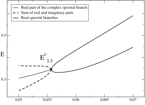
Figure 1: The crossing process of the pair of levels $(E_{6}(\hbar),E_{7}(\hbar))$ for $\hbar>h_{3}$, and the pair of levels $E^{\pm}_{3}(\hbar)$ for $\hbar<h_{3}$. A complex level $E$ is represented by $\Re E+\Im E$.

Conjecture C2 The standard sequence of nodes and antinodes of a state $\psi_{m}(\hbar)$ with m nodes, $[m/2]=n$, for $\hbar\gg\hbar_{n}>0$ and suitable labeling, is the following:

$$S_{2n}=(A_{-n-1},~{}N_{-n},\,\,...\,\,,A_{-2},~{}N_{-1},~{}A_{0},~{}N_{1},~{}A_{2},\,\,....\,\,,N_{n},~{}A_{n+1}),$$

$$S_{2n+1}=(A_{-n-1},~{}N_{-n},\,\,...\,\,,A_{-1},~{}N_{0},~{}A_{1},\,\,....\,\,,N_{n},~{}A_{n+1}).$$

There exists a parameter $\hbar_{n}^{a}>\hbar_{n}$ such that the antinode $A_{0}$ of the state $\psi_{2n}(h^{a}_{n})$ coincides with the imaginary turning point $I_{0}$ (Remark 1). There exists a parameter $\hbar_{n}^{p}>\hbar_{n}$ such that the node $N_{0}$ of the state $\psi_{2n+1}(h^{p}_{n})$ coincides with the imaginary turning point $I_{0}$ (Lemma 4). This means that at the parameter $\hbar_{n}^{a}$ and energy $E_{2n}(\hbar^{a}_{n})$ the end point of the board, $I_{0}$, touches the string. The same happens at the parameter $\hbar_{n}^{p}$ and energy $E_{2n+1}(\hbar^{p}_{n})$. Decreasing $\hbar,$ just below $\hbar^{a}_{n}$ the imaginary antinode $A_{0}$ of $S_{2n}$ doubles into the pair of non imaginary antinodes $(A_{-1},\,A_{1})$, and just below $\hbar^{p}_{n}$ the imaginary node $N_{0}$ of $S_{2n+1}$ disappears. Thus, the sequence of nodes of the state at the crossing, $\psi_{n,n}^{c}$, is,

$$S^{c}_{n,n}=(A_{-n-1},~{}N_{-n},\,\,...\,\,,N_{-1},~{}A_{-1},~{}A_{1},~{}N_{1},....\,\,,N_{n},~{}A_{n+1}),$$

and the sequences of the nodes of the states $\psi_{n}^{\pm}(\hbar)$ for $\hbar<\hbar_{n}$ are

$$S^{-}_{n}=(A_{-n-1},~{}N_{-n},\,\,...\,\,,N_{-1},~{}A_{-1}),\qquad S^{+}_{n}=(A_{1},~{}N_{1},\,\,...\,\,,N_{n},~{}A_{n+1})$$

respectively.

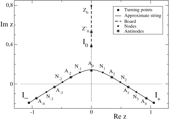
Figure 2: $\hbar>h_{3}^{a}$. The approximate monochord of $E_{6}(\hbar)$ with the nodes and antinodes.

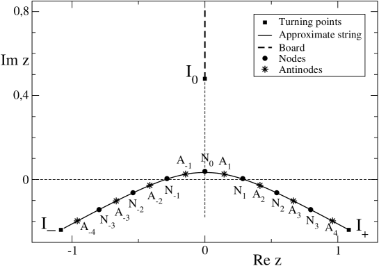
[h]

Figure 3: $\hbar>h_{3}^{p}$. The approximate monochord of $E_{7}(\hbar)$ with the nodes and antinodes.

Following the process of crossing for decreasing $\hbar,$ just after the crossing we have the breaking of both the string and the sequence of the nodes. The limit of the critical energies, $E^{c}_{n,n}\rightarrow E^{c}$ is an instability point of the Stokes complex. At the energy $E^{c}$ the exceptional Stokes line touches the short Stokes line [9], (Fig.1). We believe it is useful to try now to complete the picture of all the semiclassical behaviors of a level $E_{m}(\hbar)$ in the complex plane. It is clear that for non-real $\hbar$ other crossings of the same type are possible. Since the PT-symmetry is lost, we admit that the indexes $j,k$ of the two levels undergoing crossing are different, and their sum $j+k$ is not necessarily even. On the other side, at least one of the nodes of the state $\psi_{j+k+1}(\hbar)$ must be unstable for the crossing of $E_{j+k+1}$ with a level $E_{m}$, $m<j+k+1.$ The simplest possible generalization to the non-real $\hbar$ case is obtained if we assume that exactly one of the nodes is unstable as in the symmetric case, so that the level $E_{j+k+1}(\hbar)$ crosses the level $E_{j+k}(\hbar)$.

Conjecture C2${}^{\prime}\,$ The standard sequences of the nodes of the states $\psi_{j+k}(\hbar),\,$ $\psi_{j+k+1}(\hbar),\,$ for large $|\hbar|$, with a suitable labeling, are respectively,

$$S_{j+k}=(A_{-j-1},~{}N_{-j},\,\,...\,\,,A_{-2},~{}N_{-1},~{}A_{0}~{},N_{1},~{}A_{2},\,\,....\,\,,N_{k},~{}A_{k+1}),$$

$$S_{j+k+1}=(A_{-j-1},~{}N_{-j},\,\,...\,\,,~{}A_{-1},~{}N_{0},~{}A_{1},\,\,....\,\,,N_{k},~{}A_{k+1}).$$

There exists a parameter $\hbar_{j,k}^{a}$ such that the antinode $A_{0}$ of the state $\psi_{j+k}(\hbar_{j,k}^{a})$ coincides with the turning point of the board $I_{0}$. There exists a parameter $\hbar_{j,k}^{p}$ such that the node $N_{0}$ of the state $\psi_{j+k+1}(\hbar_{j,k}^{p})$ coincides with the turning point of the board $I_{0}$. The sequence of the nodes of the state at the crossing is,

$$S^{c}_{j,k}=(A_{-j-1},~{}N_{-j},\,\,...\,\,,N_{-1},~{}A_{-1},~{}A_{1},~{}N_{1},\,\,....\,\,,N_{k},~{}A_{k+1}),$$

and the sequences of the nodes of the states $\psi_{j}^{-}$, $\psi_{k}^{+}$ are respectively

$$S^{-}_{j}=(A_{-j-1},~{}N_{-j},\,\,...\,\,N_{-1},~{}A_{-1}),\,\qquad\,S^{+}_{k}=(A_{1},~{}N_{1},\,\,...\,\,,N_{k},~{}A_{k+1})\,.$$

[h]

Figure 4: $h_{3}<\hbar<h_{3}^{a}$. The approximate monochord of $E_{6}(\hbar)$ with the nodes and antinodes.

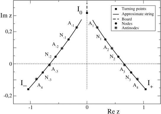
[h]

Figure 5: $h_{3}<\hbar<h_{3}^{p}$. The approximate monochord of $E_{7}(\hbar)$ with the nodes and antinodes.

Again, if we follow the process of crossing for decreasing $|\hbar|,$ after the crossing we have the breaking of the string and of the sequence of nodes and the limit of the critical energies, $E^{c}_{n,\delta_{n}}\rightarrow E^{c}(\delta)\,$ as $\,n=[(j+k)/2]\rightarrow\infty\,$ and $\,\delta_{n}=(k-j)/n\rightarrow\delta\,$, is an instability point of the Stokes complex. Thus, for complex parameter, the following crossings are possible: the two levels, $E_{j+k+(1/2)\pm(1/2)}(\hbar)$, $\,(j,k)\in\mathbb{N}^{2}\,$, cross at $\hbar_{j,k}\in\mathbb{C}^{0}$ giving two semiclassical levels $E^{-}_{j}(\hbar)$ and $E^{+}_{k}(\hbar)$ for small $|\hbar.|$

If we assume, according to the Hypothesis H2 (to be more precisely formulated in the following), that no crossing different from the above ones is possible and if we use Hypotheses H1 we obtain recursively the full picture of the Riemann sheets of the levels (Theorem 3). The level $E_{m}(\hbar),\,$ well defined and holomorphic for large $|\hbar|$, has different behaviors for $\hbar\rightarrow 0$ along different paths tangent to the real axis at $0$. Near the origin there exists a partition of $\mathbb{C}^{0}$ into a finite number of stripes, ordered for increasing imaginary part,

$$S_{-}^{m,0},~{}S_{m,0}^{m-1,0},~{}S_{m-1,0}^{m-1,1},~{}S_{m-1,1}^{m-2,1},\,\,....\,\,S_{1,m-2}^{1,m-1},~{}S_{1,m-1}^{0,m-1},~{}S_{0,m-1}^{0,m},~{}S_{0,m}^{+}$$

where the behavior of $E_{m}(\hbar)$ is respectively expressed by the following semiclassical levels in the same order

$$E_{m}^{-}(\hbar),~{}E_{0}^{+}(\hbar),~{}E_{m-1}^{-}(\hbar),~{}E_{1}^{+}(\hbar),\,\,...\,\,E_{1}^{-}(\hbar),~{}E_{m-1}^{+}(\hbar),~{}E_{0}^{-}(\hbar),~{}E_{m}^{+}(\hbar).$$

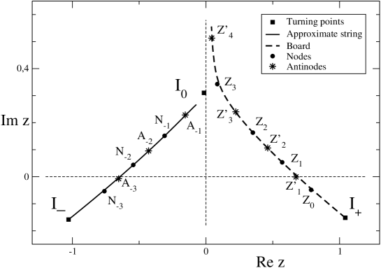
[h]

Figure 6: $0<\hbar<h_{3}$. The approximate monochord of $E_{3}^{+}(\hbar)$ with the nodes, the antinodes, the zeros and the stationary points.

To conclude, we give a brief summary of the paper content. In Sec. 2 we deal with the behavior of the levels and of the nodes for large values of $|\hbar|$. We prove a confinement of the nodes for large $\hbar>0$, the positivity of the spectrum for large $\hbar$, the reality of the states on the imaginary axis and we also consider the instability of the imaginary node of the odd states. In Sec. 3 we study the behavior of levels and states in the semiclassical limit and we show that for small $\hbar>0$ the imaginary axis is free of zeros and the nodes are bounded. We prove then the total P-symmetry breaking at the crossing. In Sec. 4 we determine the possible quantization rules and we consider the Riemann surfaces of the levels in a neighborhood of the real axis of $\hbar$. The general crossing rule and level Riemann surfaces are considered in Section 5. In the final Section 6 we introduce the string and the board, by which we determine the sequences of nodes and antinodes. We add two Appendixes concerning the semiclassical series expansions and some considerations on the numerical aspects.

2 Behavior of levels and nodes for large $|\hbar|$

The necessity of level crossing comes from the comparison of levels and states for large $\hbar$ and small $\hbar>0$. In this section we begin by investigating the principal features of levels and states for large $\hbar.$

$($a$)$ Analyticity and confinement of the nodes for large $|\hbar|$

In order to fix the number $m$ of nodes of a state $\psi_{m}(\hbar)$ for large $|\hbar|$, we prove a confinement of the nodes, so that the nodes are the only zeros in a certain region of the complex plane. For $\hbar>0$ large, it is convenient to use the representation (5) and the Hamiltonian $K(\alpha)$ so to have uniformly bounded energy and nodes. Let us consider the level $\hat{E}_{m}(0)$, $m\in\mathbb{N},$ of $K(0)\equiv K(\alpha=0)$, corresponding to the level $E_{m}(\hbar)$ of $H_{\hbar}$ at the limit of $\hbar=+\infty$ according to (7). It is important to observe that the scaling given in (7) is regular, with a positive (although unbounded) scale $\lambda=\hbar^{2/5}$ that maintains the phases on the complex plane. Due to (7) the level $\hat{E}_{m}(\alpha)$ is positive for $\alpha\in\mathbb{R}$ and $|\alpha|$. We prove now a confinement of the nodes and of the other zeros. We translate the operator $K(0)$ by $x\rightarrow x+iy,$ and we let

$$K_{y}(0)=p^{2}+i(x+iy)^{3}=p^{2}+i(x^{2}-3y^{2})x+y^{3}-3yx^{2}=p^{2}+V_{y}(x)\,\,\,.$$

We then apply the Loeffel-Martin method [1] to a level $E=\hat{E}_{m}(0)>0$, with a state $\psi=\hat{\psi}_{m}(0)$:

$$-\Im\,[\overline{\psi}(x+iy)\partial_{x}\psi(x+iy)]=\int_{x}^{\infty}\Im V_{y}(s)\,|\psi(s+iy)|^{2}ds=$$ (11)

$$\phantom{xxx}\int_{x}^{\infty}(s^{2}-3y^{2})s|\psi(s+iy)|^{2}ds=-\int^{x}_{-\infty}(s^{2}-3y^{2})s|\psi(s+iy)|^{2}ds\neq 0$$

for $\,\pm x\geq\sqrt{3}\,|y|,\,$ $y\in\mathbb{R}\,$. In this case we have a rigorous confinement of the region of the nodes

$$\mathbb{C}_{\sigma}=\{z=x+iy,\,\,y<0,\,|x|<-\sqrt{3}\,y\}\,\,\subset\,\,\mathbb{C}_{-}=\{z\in\mathbb{C},\,\Im z<0\}.$$

The same confinement extends to all $\alpha>0$ and we see that the $m$ zeros of the state $\widehat{\psi}_{m}(\alpha)$ on $\mathbb{C}_{-}$ are stable in the limit $\alpha\rightarrow+\infty,\,$ namely they are nodes by definition. Previous computations of the nodes [20] suggest that the present confinement may be sharp. Since we know the analyticity of every level $\tilde{E}_{m}(\beta)$ of $H(\beta)$ as long as the $m$ nodes of the state $\tilde{\psi}_{m}(\beta)$ are in $\mathbb{C}_{-}$, we want to look what happens at $\beta=+\infty.$ In the case of the Hamiltonian $H(\beta)=p^{2}+x^{2}+i\sqrt{\beta}x^{3},$ $\beta>0,$ by the scaling $x\rightarrow\lambda x$ with positive $\lambda=\beta^{-1/10}$, we have

$$H(\beta)\sim\beta^{1/5}(p^{2}+\beta^{-2/5}x^{2}+ix^{3})$$

so that the level $\tilde{E}_{m}(\beta)$ of $H(\beta)$, has the behavior,

$$\tilde{E}_{m}(\beta)\sim\beta^{1/5}\hat{E}_{m}(0)\,\,\,\textrm{as}\,\,\,\beta\rightarrow+\infty.$$ (12)

Thus, the operator $K(0)$ gives the asymptotic behavior of the spectrum of both the family of operators $H(\beta)$ for $\beta\rightarrow+\infty$ and the family of operators $H_{\hbar}$ for $\hbar\rightarrow+\infty$. As the nodes of the state $\hat{\psi}_{m}(0)$ are in $\mathbb{C}_{-}$, the regularized levels $\beta^{-1/5}\tilde{E}_{m}(\beta)$ are real analytic up to $\beta=+\infty$ [13]. This means the absence of level crossings at $\alpha=0.$ But a level crossing of $\hat{E}_{m}(\alpha)$ is possible at a parameter $\alpha=\alpha(m)<0.$ Therefore the level $\hat{E}_{m}(\alpha)$ is real analytic and the nodes of $\psi_{m}(\alpha)$ are in $\mathbb{C}_{-}$ for $\alpha$ in $[\alpha(m),+\infty)$. At the same time, the level $E_{m}(\hbar)$ is real analytic and the nodes of $\psi_{m}(\hbar)$ are in $\mathbb{C}_{-}$ for $\hbar$ in $[\hbar(m),+\infty)$, $\alpha(m)=-\hbar(m)^{-4/5}.$ Thus, we state a result:

Lemma 1 The level $E_{m}(\hbar)$ is real analytic and all the zeros of $\psi_{m}(\hbar)$ in $\mathbb{C}_{\sigma}$ as well as in $\mathbb{C}_{-}$ are its m nodes for $\hbar\in[\,\hbar(m),+\infty)$, where $\hbar(m)\geq 0$. All the other infinite zeros are in,

$$\mathbb{C}_{B}=\{z=x+iy,\,\,y>0,\,|x|<\sqrt{3}\,y\}\,\,\subset\,\,\mathbb{C}_{+}=\{z\in\mathbb{C},\,\Im z>0\}.$$

Therefore the levels $\hat{E}_{m}(\alpha)$ are real analytic for $\alpha\in\mathbb{R}$ for $|\alpha|$ small.

We will see that actually such zeros in $\mathbb{C}_{B}$ are imaginary.

$($b$)$ Positivity of the levels and reality of the states on the
$($b$)$ imaginary axis for large $\hbar>0$

The level $\hat{E}_{m}(\alpha)$, $m\in\mathbb{N}$ of $K(\alpha)$ is analytic in a neighborhood of the origin $U\subset\mathbb{C}$ [13, 21]. Since it is real analytic for $\alpha<0$, it is real analytic also in $U\bigcup\mathbb{R}$ [17]. The positivity of the real part of the levels comes from the numerical range and, in particular, from the kinetic energy

$$\Re\hat{E}_{m}(\alpha)=\Re\langle\widehat{\psi}_{m}(\alpha),K(\alpha)\widehat{\psi}_{m}(\alpha)\rangle=\langle\widehat{\psi}_{m}(\alpha),p^{2}\widehat{\psi}_{m}(\alpha)\rangle\,>\,0,$$

where $\psi_{m}(\alpha)$ is the corresponding normalized state. Also the level $E_{m}(\hbar)$ is real analytic and positive for $\hbar>0$ large enough. Thus, we have proved:

Lemma 2 Any given level $E_{m}(\hbar)$ is positive for large positive $\hbar$.

We now extend the analysis of the analytic states on the complex plane. Let us consider $y\in\mathbb{R}$ and the translation $f(x)\rightarrow f(x+iy)$, so that the PT-symmetric Hamiltonian becomes the isospectral PT-symmetric Hamiltonian

$$H_{\hbar}(y)=h^{2}p^{2}+i(x^{3}-(3y^{2}+1)x)-(3yx^{2}-y^{3}-y)\sim H_{\hbar}.$$ (13)

The eigenfunction $\psi_{n,y}(x)=\psi_{n}(x+iy)$ with real eigenvalue $E_{n}$ can be taken PT-symmetric on the $\mathcal{H}_{y}$ representation,

$$PT\psi_{n,y}(x)=\overline{\psi}_{n,y}(-x),$$ (14)

so that, in particular,

$$\,\,\,\psi_{n,y}(0)=\overline{\psi}_{n,y}(0)=\psi(iy).$$

Therefore, we have proved the following,

Lemma 3 If the level $\,E_{m}$, $m\in\mathbb{N},\,$ is positive then the state $\psi_{m}(z)$ extended as an entire function on the complex plane, is $P_{x}T$-symmetric,

$$(P_{x}T\psi_{m})(x+iy)=\overline{\psi}_{m}(-x+iy)={\psi}_{m}(x+iy),\,\,\quad\forall x,y\in\mathbb{R},$$ (15)

and the set of its zeros is $P_{x}$-symmetric. In particular, for a choice of the gauge, the state is real on the imaginary axis,

$$\Im\psi_{m}(iy)=0,\,\,\forall y\in\mathbb{R}.$$ (16)

$($c$)$ The nodal analysis of the process of crossing

Let us to fix $\hbar>0$ large enough and let $E=E_{m}(\hbar)$ be a positive level of the Hamiltonian (2) with a corresponding state $\psi_{m}(z)$. Now, by the complex dilation $z\rightarrow iz$, we consider the Hamiltonian on the imaginary axis:

$$H^{r}_{\hbar}=-\hbar^{2}\frac{d^{2}}{dy^{2}}+\tilde{V}(y)\,\sim\,-H_{\hbar},\,\,\qquad\tilde{V}(y)=-y^{3}-y,$$ (17)

well defined by the $L^{2}$ condition on the $x$-axis, here playing the role of the imaginary axis. The Hamiltonian $H^{r}_{\hbar}$ has the same spectrum as $-H_{\hbar},$ so that $-E=-E_{m}(\hbar)<0$ is one of its eigenvalues (Lemma 2). The corresponding state $\phi_{m}(y)=\psi_{m}(iy)$ can be taken real for $y$ real. In particular, for $y>0$ large, because of the two fundamental solutions and the reality property, we can write

$$\phi_{m}(y)\sim\frac{C}{\sqrt{p_{0}(E,y)}}\cos(p_{0}(E,y)+2\pi\alpha),\,\,$$ (18)

with a $C>0$ and where

$$p_{0}(E,y)=\sqrt{y^{3}+y-E},\qquad\alpha\in\mathbb{R}/\mathbb{Z}\,.$$

For $\,-y>0\,$ large, we have a real combinations of the two fundamental solutions,

$$\phi_{m}(y)\sim\frac{C^{\prime}}{\sqrt{p_{0}(E,y)}}\,(\exp(p_{0}(E,y))+a\exp(-p_{0}(E,y))\,),\,\,$$ (19)

with a $\,C^{\prime}>0,\,$ $p_{0}(E,y)=\sqrt{-y^{3}-y+E},\,$ $a\in\mathbb{R}.$ We consider together the two states $\psi_{m}(z)$, $[m/2]=n\in\mathbb{N}$, for a fixed $\hbar\geq\hbar_{n}$. Both the states have $n$ nodes on both the half-planes $\mathbb{C}^{\pm}$ and are distinguished by the number of imaginary nodes for $\hbar>0$ large. The whole process of crossing for $\hbar\geq\hbar_{n}$ can be studied by the behaviors of the states $\psi_{m}(z)$ with energy $E=E_{m}>0$, on the imaginary semi-axis, called the continuation of the board,

$$B^{c}(E):=\{z=iy,\,-\infty<y<\tilde{y}(E)\},$$ (20)

where the imaginary turning point is $I_{0}=i\,\tilde{y}(E)$. This means that we consider each one of the two formal states $\phi(y):=\phi_{m}(y)$, of the representation (17), for $\,y\leq{\tilde{y}}(E).\,$ For $\hbar>0$ large, we have two possible behaviors of the state $\phi(y)$ of (17). Let us recall that for $y$ in a open interval of the semi-axis $-\infty<y<\tilde{y}(E)$, if a state $\phi(y)$ is positive then it is convex; if it is negative then it is concave. On the other side, for $\,y>\tilde{y}(E)\,,$ where an eigenfunction $\phi(y)$ is positive it is also concave and where it is negative it is also convex. Since we can consider $\phi(y)$ positive decreasing for $y\ll\tilde{y}(E),$ there are only two cases:

$\phantom{i}i$)   the existence of one zero on $B^{c}(E)$,

$ii$)   the absence of zeros on $B^{c}(E)$.

Let us remark that $\tilde{y}(E)>0$ so that, by Lemma 1, a possible node on the imaginary axis should be in $B^{c}(E)$ for large $\hbar>0$. A state without imaginary nodes can have one or zero antinodes. We can state the result:

Lemma 4 Let $\,E(\hbar)$, with $\hbar>0\,$, be a positive level with a corresponding PT-symmetric state $\psi(\hbar)$. When $\hbar$ is large enough the state $\psi(\hbar)$ can have one or zero imaginary nodes.

For the existence of an imaginary node for large $\hbar>0$ we consider a state with labeling $m=2n+1$, continued to all $\hbar>\hbar_{n}>0$. An imaginary node is indeed unstable since it can cross the turning point $I_{0}$ at a parameter $\hbar_{n}^{p}>\hbar_{n}.$ For large $\hbar,$ a state $\psi(\hbar)$ with an imaginary node has no imaginary antinodes and a a state $\psi(\hbar)$ without imaginary nodes can have one or zero imaginary antinodes. It is possible and actually necessary that at a parameter $\hbar_{n}^{a}>\hbar_{n}$ the imaginary antinode disappears and two non imaginary antinodes of $\psi_{2n}(\hbar)$ are generated. We clarify this fact by a simplified example. Let $\psi_{2n}(z)=i({z^{3}}/{3}-\epsilon z)+c$, $c\neq 0$. We have $\psi^{\prime}(z)=i(z^{2}-\epsilon)=0$ at the stationary points $z_{\pm}=\pm\sqrt{\epsilon}$ and $\psi^{\prime\prime}(z)=2iz=0$ at $z=0=I_{0}$. For $\epsilon=\hbar_{n}^{a}-\hbar>0$ there are two non-imaginary antinodes and for $\epsilon<0$ there the only antinode $-i\sqrt{|\epsilon|}$ in lower complex half-plane.

3 Semiclassical limit, confinement of the nodes and the crossing rule

We now study the behavior of the levels and the states in the semiclassical limit. From the comparison with the large $\hbar>0$ behavior we will prove the necessity of the level crossings.

$($a$)$ From semiclassical to perturbation theory and semiclassical
$($a$)$ limit of the nodes

Let $\hbar\in\mathbb{C}^{0}$ with $|\hbar|$ small. Some transformations are necessary in order to use the results of [13] for the localized states. We consider Hamiltonian $H_{\hbar}$ with two wells at $x_{\pm}=\pm 1/\sqrt{3}$. We make the unitary translations centering on one of the wells or the other one, $x=x_{\pm}+y=y\pm 1/\sqrt{3},$ getting the new Hamiltonians:

$$H_{\hbar}^{\pm}=\hbar^{2}p^{2}+i(y^{3}\pm\sqrt{3}y^{2})\mp\textsl{E},\,\qquad\textsl{E}=i\frac{2}{3\sqrt{3}}.$$

We make the suitable dilations in order to use the perturbation theory [13]. We put

$$y=\lambda^{\pm}(\hbar)z,\,\qquad\lambda^{\pm}(\hbar)=\exp(\mp i\pi/8)3^{-1/8}\sqrt{\hbar}\,$$ (21)

and we get

$$H_{\hbar}^{\pm}\sim\hbar c^{\pm}H(\beta^{\pm}(\hbar))\mp\textsl{E}\phantom{xxxxxxxx}$$ (22)

where

$$c^{\pm}=3^{1/4}\sqrt{\pm i},\,\,\qquad\beta^{\pm}(\hbar)=\exp(\mp i5\pi/4)3^{-5/4}\hbar,$$

and where $H(\beta)$ is

$$H(\beta)=p^{2}+x^{2}+i\sqrt{\beta}x^{2}.\phantom{xxxi}$$ (23)

Let us notice that the parameters $\beta^{\pm}(\hbar)$ are not in the cut plane

$$\mathbb{C}_{c}=\{z\in\mathbb{C};\,\,z\neq 0,\,\,|\arg z|<\pi\},$$

so that we cannot use all the results of [13]; nevertheless we can use some of the results of [18]. It is clear from the perturbation theory that we have the semiclassical behavior of the levels,

$$E_{n}^{\pm}(\hbar)=\mp i\textsl{E}+\hbar c^{\pm}(2n+1)+O(\hbar^{2}),\,\,\hbar>0.$$ (24)

In the perturbation theory of Hamiltonian (23) we have the relevant fact that in the semiclassical limit all the nodes of the state $\tilde{\psi}_{n}(\beta^{\pm}(\hbar))$ go to the short Stokes line $\,[\,-\sqrt{2n+1},\sqrt{2n+1}\,\,].$ In the semiclassical limit this corresponds respectively to the wells $x_{\pm}$ of the nodes of the semiclassical states $\psi_{n}^{\pm}(\hbar)$,

Lemma 5 Both the states $\psi_{n}^{\pm}(\hbar)$ have $n$ zeros tending to the points $x_{\pm}$, respectively, as $\hbar\rightarrow 0^{+}$.

We will prove a stable confinement of the zeros of both the states $\psi_{n}^{\pm}(\hbar)$ in $\mathbb{C}^{\pm}$ (10) respectively, so that such zeros coincide with the nodes. Thus, we will prove that no crossing between the levels of the same set $\{E_{n}^{-}(\hbar\}_{n\in\mathbb{N}}$ or of the same set $\{E_{n}^{+}(\hbar\}_{n\in\mathbb{N}}$ can occur, contrary to crossings of the levels of $\{E_{n}^{-}(\hbar)\}_{n\in\mathbb{N}}$ with the levels of $\{E_{n}^{+}(\hbar\}_{n\in\mathbb{N}}$ that are indeed possible.

$($b$)$ The confinements of the nodes and the crossing rule

Let us consider $\hbar>0$ and a level $E\in\mathbb{C},$ with the corresponding state $\psi(z),$ and $\psi(iy)=\phi(y),$ $z,y\in\mathbb{C}$. We transform the Hamiltonian (17) by imaginary translations:

$$H^{r}_{\hbar}(x)=-\hbar^{2}\frac{d^{2}}{dy^{2}}+\tilde{V}(y-ix),\,$$

$$\tilde{V}(y-ix)=\Re\tilde{V}(y-ix)+i\Im\tilde{V}(y-ix)=-(y-ix)^{3}-(y-ix)\vrule height=7.20003pt,width=0.0pt,depth=7.20003pt$$ (25)

$$\phantom{\tilde{V}(y-ix)}=-y^{3}+3x^{2}y-y+i(x(3y^{2}+1)-x^{3})$$

where $\,\Im\tilde{V}(y-ix)=(x(3y^{2}+1)-x^{3}\,)$ with level $\,-E\,$, for a fixed $x\neq 0$. We consider a state,

$$\phi_{x}(y)=\phi(y-ix),\,\,\,\,\,n\in\mathbb{N},$$

with the well known asymptotic behavior(18),

$$\phi_{x}(y)\sim\frac{C}{\sqrt{p_{0}(E,w)}}\cos(p_{0}(E,w)+\theta),\,\quad w=y-ix,\,\quad y\rightarrow+\infty,$$

for a $\,C>0,\,$ $\theta\in\mathbb{R}/2\pi\mathbb{Z}\,$ and

$$|\phi_{x}(y)|^{2}=O(|y|^{-3/2})\,\,\quad\textrm{for}\,\quad y\rightarrow+\infty.$$

Since the dominant term is bounded and real, we have,

$$\Im(\bar{\phi}(y)\partial_{y}\phi(y))\rightarrow 0,\,\quad\textrm{as}\,\quad y\rightarrow+\infty.$$

We consider the Loeffel-Martin formula in order to generalize to our problem the expression of the imaginary part of a shape resonance:

$$\,\Im\,(\hbar^{2}\overline{\phi}(y)\partial_{y}\phi(y))=-\Im E\,\int^{\infty}_{y}|\phi(s)|^{2}ds,\,\,\forall y\in\mathbb{R},$$ (26)

where the integral in (26) exists and is bounded for the semiclassical behavior. Thus we state the result:

Lemma 6 Let us consider the non-real levels $E^{\pm}_{n}(\hbar)$ at a fixed value of the parameter $\hbar<\hbar_{n}$. The corresponding states $\psi_{n}^{\pm}(z)$ are different from $0$ on the imaginary axis and, being entire functions, they are free of zeros in a neighborhood of the imaginary axis. Obviously, the width of this neighborhood is not uniform at infinity.

We next apply the Loeffel-Martin method [1] generalized to the case of diverging integrals:

$$\Im\,[\hbar^{2}\overline{\phi}_{x}(y)\,\partial_{y}\phi_{x}(y)]=\Im\,[\hbar^{2}\overline{\phi}_{x}(y_{0})\partial_{y}\phi_{x}(y_{0})]+\vrule height=7.20003pt,width=0.0pt,depth=7.20003pt$$ (27)

$$\phantom{\Im\,[\hbar^{2}\overline{\phi}_{x}(y)]}\int_{y_{0}}^{y}(x(3s^{2}+1-x^{2})+\Im E)|\phi_{x}(s)|^{2}ds\rightarrow+\infty,$$ (28)

as $y\rightarrow+\infty$ for fixed $y_{0},x\in\mathbb{R},$ $x\neq 0.$ We know that the zeros, for large $|z|$, have the asymptotic direction $\arg z\rightarrow\pi/2$ [13]. Let $E\in\mathbb{C}_{\pm}$ be a non real level with state $\psi(z)$ of the Hamiltonian $H_{\hbar}$ for a fixed $\hbar>0$. In the regions

$$\Omega^{\pm}=\{z=x+iy\in\mathbb{C}^{\pm},\,\,x^{2}\leq 3y^{2}+1,\,\,y>0\,\},$$

for $E\in\mathbb{C}_{\pm}$ respectively, there are no zeros for large $y$. Let for instance $\Im E>0$, $y_{0}>0$; by (28) we have the absence of a zero at $(x,y)$ for $0<x<1$ and $y>y(x)$ for a function $y(x)>y_{0}$. The function $y(x)$ is not uniformly bounded for $x$ small, but this is not a problem because of Lemma 6. This means that the large zeros are on $\mathbb{C}^{\mp}$ if $E\in\mathbb{C}_{\mp}$, respectively. In the limit of $\hbar\rightarrow\hbar_{n}^{-}$ the energies $E_{n}^{\pm}(\hbar)$ become positive, and the large zeros of $\psi_{n}^{\pm}(\hbar)$ become imaginary. We are then able to state a stronger condition on the asymptotics of the zeros:

Lemma 7 Since $E_{n}^{\pm}(\hbar)\in\mathbb{C}_{\mp}$, the $n$ nodes of the two states $\psi_{n}^{\pm}(\hbar)$, near $x_{\pm}$ for small $\hbar$, stay respectively in $\mathbb{C}^{\pm}$ for all $\hbar<\hbar_{n}$. Since the state $\psi_{n}^{+}(\hbar)$ $(\psi_{n}^{-}(\hbar))$ is the only one to have $n$ nodes in $\mathbb{C}^{+}$ $(\mathbb{C}^{-})$, the two functions $E_{n}^{\pm}(\hbar)$ are analytic for $0<\hbar<\hbar_{n}.$ At the crossing limit, the two levels $E_{n}^{\pm}(\hbar)$ with the states $\psi_{n}^{\pm}(\hbar)$, coincide. The state $\psi_{n,n}^{c}$ at the crossing is $PT$-symmetric and has $2n$ non-imaginary zeros conventionally considered the only nodes. The large zeros are imaginary.

Proof.. We have, $\psi_{n}^{+}(\hbar)=PT\psi_{n}^{-}(\hbar)$ for $\hbar<\hbar_{n}$, and $\psi_{n}^{\pm}(\hbar)\rightarrow\psi_{n,n}^{c}$ as $\hbar\rightarrow\hbar_{n}^{-}$, so that $\psi_{n,n}^{c}=PT\psi_{n,n}^{c}.$ The state $\psi_{n}^{+}(\hbar)$ has only $n$ zeros in $\mathbb{C}^{+}$ and the state $\psi_{n}^{-}(\hbar)$ has only $n$ zeros in $\mathbb{C}^{-}$. Since at the limit $\hbar\rightarrow\hbar_{n}^{-}$ these zeros cannot diverge or become imaginary, all the limits of the non-imaginary zeros of both the state $\psi^{\pm}(\hbar)$ are all the non-imaginary zeros of the limit state $\psi_{n,n}^{c}.$

We say conventionally that the $2n$ non-imaginary zeros are the nodes of $\psi_{n,n}^{c}.$

Consider a state $\psi_{m}(\hbar)$, for $\hbar>\hbar_{n}$ having limit $\psi_{n,n}^{c}$ as $\hbar\rightarrow\hbar_{n}^{+}$. We have:

Lemma 8 Let $\psi_{m}(\hbar)$, for $\hbar>\hbar_{n}$, be a generic state having limit $\psi_{n,n}^{c}$ as $\hbar\rightarrow\hbar_{n}^{+}.\,$ For $\hbar>\hbar_{n},\,$ $\psi_{m}(\hbar)$ has exactly $2n$ non-imaginary zeros, possible nodes, stable at $\hbar_{n}$. Taking into account the possible existence of one imaginary node, the number $m$ of its nodes is not greater than $2n+1$.

Proof.. For $\hbar>\hbar_{n}$, both the states $\psi_{m}(\hbar)$ are PT-symmetric and the corresponding levels $E_{m}(\hbar)$ are positive (Lemma 2 and 3). Because of the symmetry and the simplicity of the spectrum, a non-imaginary zero cannot become imaginary and an imaginary zero cannot leave the imaginary axis. Due to (28), a non-imaginary zero of $\psi_{m}(\hbar)$, with energy $E=E_{m}(\hbar),$ can go to infinity along a path asymptotic to the imaginary axis at infinity. But at any fixed $\hbar>\hbar_{n}$ the state $\psi_{m}(\hbar)$ has the following behavior in a neighborhood of the imaginary axis (18),

$$\psi_{m}(z)=\phi_{m}(w)\sim\frac{C}{\sqrt{p_{0}(E,w)}}\cos(p_{0}(E,w)+\alpha),\,\,w=y-ix,\,\,y\rightarrow+\infty,$$

for a $C>0,$ $p_{0}(E,w)=\sqrt{w^{3}+w-E},$ $\alpha\in\mathbb{R}/\mathbb{Z},$ so that it is free of zeros for a small $|x|\neq 0,$ $x\in\mathbb{R}$ and $y>0$ large enough.
The number of non-imaginary nodes of both the states $\psi_{m}(\hbar)$ is $2n$ as the state $\psi^{c}_{n,n}$. All the non-imaginary zeros can go to the half plane $\mathbb{C}_{-}$ for large $\hbar>0$, as the nodes do. We know that only one of the imaginary zeros can be a node (Lemma 4). Thus, the maximum number of nodes is $2n+1,$ whereas the minimum number is $0.$ Because of the independence of the two states $\psi_{m}(\hbar)$ having limit $\psi_{n,n}^{c}$ as $\hbar\rightarrow\hbar_{n}^{+},$ the maximal values of the pair of numbers $m$ is $(2n,2n+1)$.

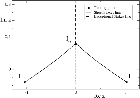
Figure 7: $\hbar=0$. The monochord, the subset of the Stokes complex, consisting of the short Stokes line (string) and the exceptional Stokes line (board), at the critical energy $E^{c}=0,35226..$.

Actually, considering the sequence of pairs of levels $E_{m}(\hbar)>0$ obtained by the crossings for large $\hbar>0$, only the the maximum values of the pairs of number $m$, $(2n,2n+1)$ are compatible with the uniqueness of each level. Only the sequence of pairs,

$$(E_{0},E_{1}),(E_{2},E_{3}),(E_{4},E_{5}),...,$$

gives exactly the full sequence of levels $E_{0},E_{1},E_{2},...$. The imaginary node of the state $\psi_{2n+1}(\hbar)$ is always imaginary but can well coincide with the lowest imaginary zero of $\psi_{2n}(\hbar)$ at $\hbar=\hbar_{n}.$

Thus, we state the following,

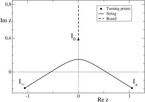
Figure 8: $\hbar$=0. Instability of the monochord for a positive variation of the energy: $E>E^{c}$.

Theorem 1 For each $n\in\mathbb{N}$, there exists a parameter $\hbar_{n}>0$ and a crossing at $\hbar_{n}$. The two levels $E_{2n+(1/2)\pm(1/2)}(\hbar)$ separated for $\hbar>\hbar_{n}$, and the two levels $E_{n}^{\pm}(\hbar_{n})$ separated for $\hbar<\hbar_{n}$, crosses at $\hbar_{n}>0.$ The two states $\psi_{2n+(1/2)\pm(1/2)}(\hbar)$, $\hbar\gg\hbar_{n},$ have a set of $2n$ non-imaginary nodes.

Proof.. The existence of the crossings is necessary because of the positivity of the analytic functions $E_{m}(\hbar)$ for large $\hbar>0,$ and the non reality of the analytic functions $E_{n}^{\pm}(\hbar)$ for small $\hbar>0$. In particular, if seen from $\hbar\leq\hbar_{n}$, we have a crossing between the levels $E_{n}^{\pm}(\hbar)$ when they becomes real and equal. The crossing between the levels $E_{2n}(\hbar)$, $E_{2n+1}(\hbar)$ is possible because the stability of the $2n$ non-imaginary nodes of both the states $\psi_{2n+(1/2)\pm(1/2)}(\hbar)$ and the instability of the imaginary node of the state $\psi_{2n+1}(\hbar)$. Because of the $P_{x}T$-symmetry of both the states $\psi_{2n+(1/2)\pm(1/2)}(\hbar)$, they have $n$ nodes in both the half-planes $\mathbb{C}^{\pm}$. The continuation to $\hbar<\hbar_{n}$ of the $n$ nodes in $\mathbb{C}^{\pm}$ are the nodes of the states $\psi_{n}^{\pm}(\hbar)$ in $\mathbb{C}^{\pm}$, respectively.

Remark 1 The zeros on the upper half-plane for large $\hbar>0$ are all imaginary.

This statement strengthens the confinement of the zeros for large $\hbar>0$ obtained above. It ensues from the result that all the non-imaginary zeros are nodes, and all the nodes are in the lower half-pane for large $\hbar>0.$

Conjecture C3 The sequence $\hbar_{n}$ has a vanishing limit for $n\rightarrow\infty$.

This conjecture is based on the semiclassical and the exact semiclassical theory. It is related to the conjecture that $n\hbar_{n}$ and $2n\hbar_{n}$ tend to the action integral of single well $J^{+}(E^{c},0)=J^{-}(E^{c},0)$ and of double well $J_{2}(E^{c},0)$, respectively, as $n\rightarrow\infty$ (31), (34). The instability of the nodes is related to the contact of the string with the board and the instability of the string at $E=E^{c}$, $\hbar=0.$ For the possibility of proving this conjecture by perturbation theory see [22, 23, 24].

Also the behavior of the isolation distance for large $\hbar$ and large $n$ agrees with this conjecture.

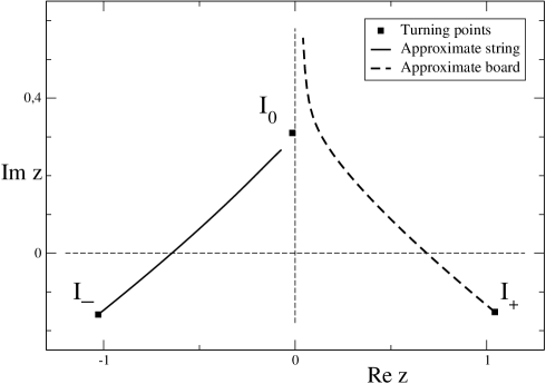
Figure 9: $\hbar=0$. Instability of the monochord for a complex variation of the energy: $E\neq\bar{E}$.

$($c$)$ The total P-asymmetry at the crossing

We have seen that the states $\tilde{\psi}_{n}=\tilde{\psi}_{n}(0)$ of $H(\beta)$ at fixed $\beta=0,$ have definite parity: $P\tilde{\psi}_{n}=(-1)^{n}\tilde{\psi}_{n}$. This means that $|\tilde{\psi}_{n}|^{2}$ is $P$-symmetric, and the expectation value of the parity is $\,\langle\tilde{\psi_{n}},P\tilde{\psi_{n}}\rangle=(-1)^{n}$. We want to prove that the state at the crossing, $\psi_{n}^{c}=\psi_{n}(\hbar_{n})$, $n\in\mathbb{N},$ has vanishing mean value of the parity, $\langle\psi_{n}^{c},P\psi_{n}^{c}\rangle=0,\,$ so that it is totally $P$-asymmetric in the sense that $\psi_{n}^{c}$ is orthogonal to $P\psi_{n}^{c}$.

We have a crossing of $\,E_{n}^{\pm}(\hbar)\,$ at $\,\hbar=\hbar_{n}\,$ when $\,\Im E_{n}^{\pm}(\hbar)=0.\,$ For $0<\hbar<\hbar_{n},$ the two clamped points of $\psi_{n}^{\pm}$ are $(I_{\mp},I_{0})$ respectively. At the crossing, we have $P_{x}$ symmetry of the turning points, so that $I_{-}=\bar{I_{+}},$ $I_{0}=-\bar{I_{0}}$.
Let $\,H=H_{\hbar},\,$ $\,H_{\hbar}^{*}=\bar{H}=H_{\bar{\hbar}},\,$ with two levels  $E_{j}=\bar{E}_{j}\,$ and states $\,\psi_{j},\,$ $j=1,2\,$. Then

$$H\psi_{1}=E_{1}\psi_{1},\,\,\,\qquad\bar{H}\bar{\psi}_{2}=E_{2}\bar{\psi}_{2},$$

so that

$$\langle\bar{\psi}_{2},H\psi_{1}\rangle=E_{1}\,\langle\bar{\psi}_{2},\psi_{1}\rangle=E_{2}\,\langle\bar{\psi}_{2},\psi_{1}\rangle$$ (29)

and, by subtraction

$$0=(E_{2}-E_{1})\,\langle\psi_{1},\bar{\psi}_{2}\rangle\,.$$

Let now to vary the semiclassical parameter $\hbar$, so that:

$$0=(E_{2}(\hbar)-E_{1}(\hbar))\,\langle\psi_{1}(\hbar),\bar{\psi}_{2}(\hbar)\rangle,$$

for $\hbar>0.$ If $E_{1}(\hbar)\neq E_{2}(\hbar)$ for $\hbar>\hbar_{n},$ and $E_{1}(h^{+}_{n})=E_{2}(h^{+}_{n})=E,$ $\psi_{1}(h^{+}_{n})=\psi_{2}(h^{+}_{n})=\psi,$ we have

$$0=\langle\psi,\bar{\psi}\rangle=\langle\psi,P\psi\rangle=\int_{\mathbb{R}}\psi^{2}(x)dx.$$ (30)

We have thus proved:

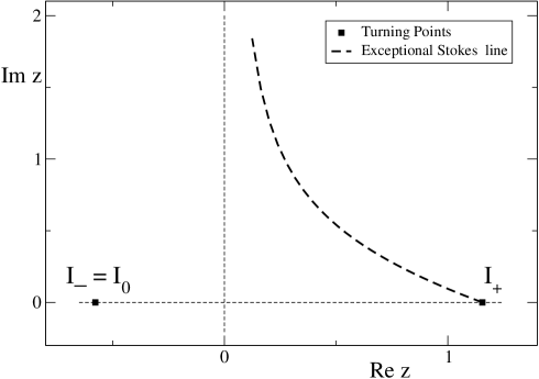
[h]

Figure 10: $\hbar=0$. The monochord at the semiclassical energy $E_{n}^{-}(0)=i2/3\sqrt{3}$, $\forall n\in\mathbb{N}$. The string is the point $I_{-}=I_{0}=x_{-}.$

Lemma 9 The PT-symmetric state at the crossing point,

$${\psi}^{c}_{n,n}=\psi_{2n+1}(h^{+}_{n})=\psi_{n,n}(h^{+}_{n})=PT{\psi}^{c}_{2n},$$

is completely P-asymmetric, namely $\langle{\psi}^{c}_{n,n},P{\psi}^{c}_{n,n}\rangle=0.$

Considering the states as eigenfunctions of the Hamiltonian $K(\alpha)$, the state $\psi=\hat{\psi}_{2n+1}$ is odd in the sense that it gives a negative mean value of the parity operator , $\langle\psi,P\psi\rangle<0$ tending to $-1$ in the limit $\alpha\rightarrow+\infty.$ Conversely, the state $\psi=\hat{\psi}_{2n}$ is even since $\langle\psi,P\psi\rangle>0$ and tends to $1$ in the limit $\alpha\rightarrow+\infty\,.$ Thus, the crossing of two levels with states of opposite parities for large $\alpha$, is possible.

4 The boundedness of the levels and the Riemann surfaces

In this section we examine the possible types of quantization rules excluding the divergence of the levels. We then consider the properties of the Riemann surfaces of the eigenvalues in the neighborhood of the real axis.

$($a$)$ The quantization rules and the boundedness of the levels

There are two types of rigorous quantization rules for $\hbar>0$ giving the boundedness of the levels for bounded $\hbar.$ Moreover, there is another rigorous quantization rule for large $\hbar>0.$ We have seen that there are two kinds of confinement of the nodes depending on two conditions for the energy: if the energy level satisfies the condition $E\in\mathbb{C}^{\mp}$ then the set of $n$ nodes of the corresponding state $\psi$ is confined on $\mathbb{C}^{\pm}$ respectively. Thus, both the levels $E_{n}^{\pm}(\hbar)$, $\hbar<\hbar_{n},$ satisfy the unique conditions on the phase and on the nodes, do not cross and are analytic. We have two kinds of quantization rules for a fixed $\hbar<\hbar_{n}$, giving the levels $E_{n}^{\pm}$ and the states $\psi_{n}^{\pm}$. At $\hbar=\hbar_{n}$, the two levels become positive and we have the crossing.

Suppose there exist two continuations of both levels $E_{n}^{\pm}(\hbar)$, $n\in\mathbb{N},$ from $\hbar<\hbar_{n}$ to $\hbar>\hbar_{n}.$ For the moment we maintain the same names $E_{n}^{\pm}(\hbar)$ for the continuations of the levels, even if such continuations should be distinguished by different labeling We know that both continuations of the energy levels are positive and both continuations of the states have $n$ nodes in both $\mathbb{C}^{\pm}.$ There exist two regular circuits $\gamma^{\pm}$ such that

$$P_{x}\gamma^{+}=\gamma^{-},\qquad\gamma^{\pm}=\partial\Omega^{\pm},$$

where $\Omega^{\pm}$ are regular regions large enough, with

$$\Omega^{\pm}\subset\mathbb{C}^{\pm}=\{x+iy,\,\pm x>0,\,y\in\mathbb{R}\}\,.$$

and the exact quantization conditions read

$$\frac{1}{2i\pi}\oint_{\gamma^{\pm}}\frac{\psi^{\prime}(z)}{\psi(z)}dz=n\,.$$

We can better write

$$J^{\pm}(E,\hbar):=\frac{\hbar}{2i\pi}\oint_{\gamma^{\pm}}\frac{\psi^{\prime}(z)}{\psi(z)}dz+\frac{\hbar}{2}=\hbar\Bigl{(}n+\frac{1}{2}\Bigr{)},$$ (31)

if $\psi(z)=\psi_{n}^{\pm}(\hbar,z)$ and $E=E_{n}^{\pm}(\hbar)\in\mathbb{C}^{\mp}\,$ respectively.

In particular, for small $\hbar>0,$ and fixed $n\in\mathbb{N},$ the quantization rules (31) become the semiclassical quantization conditions for $E=E_{n}^{\pm}(\hbar)$ ,

$$J(E,\hbar)=\frac{1}{2i\pi}\oint_{\gamma^{\pm}}p_{0}(E,z)dz+O(\hbar^{2})=\hbar\Bigl{(}n+\frac{1}{2}\Bigr{)},$$ (32)

where $p_{0}(E,z)=\sqrt{V(z)-E},$ and the paths $\gamma^{\pm}$ shrink around the short Stokes line. Both the quantization conditions (31) at $\hbar=\hbar_{n}$ give the same solution $E_{n}^{c}$, $\psi_{n}^{c}$, and for $\hbar>\hbar_{n}$ both give the both the solutions $E_{m}(\hbar)$, $\psi_{m}(\hbar)$, $[m/2]=n\in\mathbb{N}.$

We distinguish the two solutions by the selecting condition

$$E_{2n+1}(\hbar)>E_{2n}(\hbar).$$ (33)

Therefore both functions $E_{m}(\hbar)$ are analytic for $\hbar>\hbar_{n}.$ For a fixed, large $\hbar\gg\hbar_{n}$ we have the exact quantization rules,

$$J_{2}(E,\hbar):=\frac{\hbar}{2i\pi}\oint_{\Gamma}\frac{\psi^{\prime}(z)}{\psi(z)}dz+\frac{\hbar}{2}=\hbar(m+\frac{1}{2}),$$ (34)

where the solutions are,

$$\psi(z)=\psi_{m}(\hbar,z),\,\quad E=E_{m}(\hbar),\,\quad m=2n\,\,\textrm{or}\,\,2n+1,\,\quad\Gamma=\Gamma_{m}=\partial\Omega_{m},$$

and where $\Omega_{m}\subset\mathbb{C}_{-}$ is large enough in order to contain all the $m$ nodes.

These quantization conditions (31), (34) yield the boundedness and the continuity of the levels even at the crossing point $\hbar_{n}$.

Lemma 10 $(a)$ The two functions $E_{n}^{\pm}(\hbar),$ are analytic for $\hbar<\hbar_{n}$. The two functions $E_{m}(\hbar)$, $[m/2]=n$ are analytic for $\hbar>\hbar_{n}$.
$(b)$ Let $E(\hbar)$, be one of the two functions $E_{n}^{\pm}(\hbar),$ $n\in\mathbb{N}$ for $\hbar\leq\hbar_{n}$ with one of its two continuations $E_{m}(\hbar)$, $[m/2]=n$ for $\hbar>\hbar_{n}$. The function $E(\hbar)$ is bounded and continuous on $\mathbb{R}_{+}$ and is analytic with a square root singularity at ${\hbar}_{n}$.

Proof.. The point ($a$) is proved by the exact quantization conditions (31) with the selection condition (33) for $\hbar>\hbar_{n}$.

We prove by absurd point($b$). We assume the divergence of $E(\hbar)$ at $h^{c}\gg\hbar_{n}$ where the $m$ nodes of the corresponding state are in $\mathbb{C}_{-}$. The extension to the general case is simple. We consider the operator,

$$\frac{H_{\hbar}-E(\hbar)}{|E(\hbar)|}\sim{\hat{\hbar}}^{2}\,p^{2}+ix^{3}-i\delta x-\eta,$$

by a scaling $x\rightarrow\lambda x,$ $\lambda=|E|^{1/3}$, where ${\hat{\hbar}}=\hbar|E^{-5/3}|,$ $\delta=|E|^{-2/3}$, $\eta=E/|E|$, $|\eta|=1$. For small ${\hat{\hbar}}>0,$ by simply putting $\delta=0,$ we have the semiclassical quantization condition,

$$\frac{1}{2i\pi}\oint_{\Gamma_{m}}\sqrt{iz^{3}-\eta}\,\,dz={\hat{\hbar}}\Bigl{(}m+\frac{1}{2}\Bigr{)}+O({\hat{\hbar}}^{2}),$$ (35)

where $\Gamma_{m}=\partial\Omega_{m}$ and all the $m$ nodes are in $\Omega_{m}\subset C_{-}.$ It is easy to see that (35) can be satisfied only if $\eta\rightarrow 0$ as ${\hat{\hbar}}\rightarrow 0.$

$($b$)$ The Riemann surfaces near the real axis

Let us consider the sector (3) on the $\hbar$ complex plane,

$$\mathbb{C}^{0}=\{\hbar\in\mathbb{C};\,\hbar\neq 0\,,\arg(\hbar)<\pi/4\},$$

and the Riemann sheet $\mathbb{C}^{0}_{m}$ of the level $E_{m}(\hbar)$, $n=[m/2]$, defined in $\mathbb{C}^{0},$ with a square root singularity at $\hbar_{n}$ and a cut, $\gamma_{n,n}=(0,\hbar_{n}\,]\,$. We prove the following:

Theorem 2 The levels $(E_{2n+1}(\hbar),E_{2n}(\hbar))$ are analytic functions defined on the Riemann sheets $(\mathbb{C}^{0}_{2n},\,\,\mathbb{C}^{0}_{2n+1})$ respectively, both of them having only the cut $\gamma_{n,n}=(0,\hbar_{n}\,]$ on the real axis. The positive analytic functions $(E_{2n+1}(\hbar),E_{2n}(\hbar)),$ with $E_{2n+1}(\hbar)>E_{2n}(\hbar)$ on $(\hbar_{n},+\infty)$ take the following values at the boundaries of the cut:

$$E_{2n}(\hbar\pm i0^{+})={E}^{\pm}_{n}(\hbar),\,\,E_{2n+1}(\hbar\pm i0^{+})={E}^{\mp}_{n}(\hbar),\,\,\forall\,\,0<\hbar<\hbar_{n}.$$ (36)

Proof.. Since both the functions $(E_{2n+}(\hbar),E_{2n}(\hbar))$ have a square root singularity at $\hbar_{n},$ and

$$E_{2n+1}(\hbar_{n}+\epsilon)-E_{2n}(\hbar_{n}+\epsilon)=O(\sqrt{\epsilon})>0,$$

for $\epsilon>0$ small,

$$\pm\Im(E_{2n+1}(\hbar_{n}+\exp(\pm i\pi)\epsilon)-E_{2n}(\hbar_{n}+\exp(\pm i\pi)\epsilon))<0,$$

and $\mp\Im E_{n}^{\pm}(h)>0,$ for $h<\hbar_{n},$ we necessarily have,

$$E_{2n+1}(\hbar_{n}+\exp(\pm i\pi)\epsilon)={E}^{\mp}_{n}(\hbar_{n}-\epsilon),$$

$$E_{2n}(\hbar_{n}+\exp(\pm i\pi)\epsilon)={E}^{\pm}_{n}(\hbar_{n}-\epsilon).$$

Remark 2 Let us consider the crossing process along a path starting from $\hbar=0$, turning around the singularity at $\hbar_{n}$ and going back at $\hbar=0.$ The state $\psi_{n}^{+}(\hbar)$ concentrated at $x_{+}$ at the beginning of the path, becomes the state $\psi_{n}^{-}(\hbar)$ concentrated at $x_{+}.$ Now, we consider a path starting at large $\hbar>0,$ turning around $\hbar_{n}$ and going back to a large $\hbar>0$. An odd state $\psi_{2n+1}(\hbar)$ at the beginning of the trip becomes an even state $\psi_{2n}(\hbar)$: the imaginary node of the lower half plane becomes an imaginary zero of the upper half plane.

Remark 3 The Riemann sheet $\mathbb{C}^{0}_{0}$ of the fundamental level has only one cut $\gamma_{0,0}=[0,h_{0}]$ on $\mathbb{R}$ [9], and the discontinuity on the cut is defined by the rule,

$$E_{0}(\hbar\pm i0^{+})={E}^{\pm}_{0}(\hbar),\,\,\forall\,\,\hbar,\,\,0<\hbar<h_{0}.$$ (37)

We recall, for instance, that $E_{0}^{+}(\hbar)=E_{0}(\hbar+i0)$, is defined as the limit from above for small $\hbar>0.$ This definition extends directly to all $\hbar>0$ in the absence of complex singularities. Formula (37) means that the absence of other singularities involving the function $E_{0}(\hbar)$ is possible. Thus, by using the Hypothesis H1, we assume that in $\mathbb{C}_{0}^{0}$ there is only the cut $\gamma_{0,0}$.

5 The general crossing rule for complex $\,{\boldsymbol{\hbar}}\,$ and the Riemann surfaces of the levels

We extend the study to the general case of $\hbar\in\mathbb{C}^{0}$ where it is more difficult to prove the selection rules. The potential $V(x)=i(x^{3}-x)$ is PT-symmetric with two wells at $x_{\pm}=\pm 1/\sqrt{3}$ respectively. Let us consider the parameter $\alpha$ along a line defined by a fixed $c\in\mathbb{R}$, $\{\alpha=-r+ic,\,\forall r>0\}$. The corresponding line on the $\hbar$ complex plane,

$$\gamma_{c}=\{\hbar=(r+ic)^{-4/5},\,r>0\},$$ (38)

is tangent to the real axis at the origin.The choice of these kind of paths is arbitrary but is justified by the semiclassical analysis of the crossings in the $\alpha$ complex plane.

For $\hbar$ in the line $\gamma_{c}$, $c\neq 0$, we still have a double well but the PT-symmetry of the Hamiltonian is broken. For a fixed $c\neq 0$ and a large $r>0$ we expect the existence of the levels $E_{j}^{\pm}(\hbar)$ and the $j$-nodes states $\psi_{j}^{\pm}(\hbar)$ localized in the $x_{\pm}$ well respectively [18]. Even if there are no crossings in $\gamma_{c}$ for a $c\neq 0$, with $|c|$ small, it is clear that continuing the level $E_{j}^{\pm}(\hbar)$ and the state $\psi_{j}^{\pm}(\hbar)$, up to $r>0$ small enough, the state becomes delocalized and should change name. The delocalized states for $|\hbar|$ large are called $\psi_{m}(\hbar)$ for an $m\geq j$ to be specified. In this case, we expect that the continuation of $\psi_{j}^{\pm}(\hbar)$ is $\psi_{m}(\hbar)$ with an $m\geq j$ to be discussed. On the other side, if we start with a $\psi_{m}(\hbar)$, $\hbar\in\gamma_{c}$ for a small $r>0,$ if $c>0$ is large enough, we expect to have no crossings for all $r>0$, and $\psi_{m}(\hbar)$ becomes $\psi^{+}_{m}(\hbar)$ for $r>0$ large.

We now consider the Riemann sheet of the level $E_{m}(\hbar)$ for large $|\hbar|$ and continued on all the sector $\hbar\in\mathbb{C}^{0}$. We always assume the minimality condition on the number of crossings (Hypothesis H1). Thus we extend the result of Lemma 9 end we assume,

Hypothesis H2 The generalization of the crossings to non positive $\hbar$ and different indexes $(j,k)\in\mathbb{N}^{2}$ is the natural one. On one side $E_{j+k}(\hbar)$ crosses $E_{j+k+1}(\hbar)$ and on the other side $E^{+}_{j}(\hbar)$ crosses $E^{-}_{k}(\hbar)$ at the same parameter $\hbar_{j,k}\in\mathbb{C}^{0}.$

The Hypothesis H2, difficult to prove, is the simplest generalization of Theorem 1 concerning the case of $j=k=n$ for positive $\hbar_{n,n}=\hbar_{n}>0.$ We will see (Theorem 3) that with this rule we can have a minimal structure of singularities (in agreement with Hypothesis H1).
We define the Riemann sheet of the eigenvalue $E_{m}(\hbar)$, $m\in\mathbb{N},$ holomorphic for large $|\hbar|$, with the minimal number of branch points and cuts for small $|\hbar|$.
We call $\gamma_{\pm}$ the boundary lines of the sector $\mathbb{C}^{0},\,$ $\gamma_{\pm}=\sqrt{\pm i}\mathbb{R}_{+}.$ Because of the results of [13], we have the identity of two definitions at each side: $E_{m}(\hbar)=E_{m}^{\pm}(\hbar)$ for $\hbar\in\gamma_{\pm}$ respectively.

Let us consider the Riemann sheet $\mathbb{C}^{0}_{0}$ of $E_{0}(\hbar),$ with only one positive singularity at $\hbar_{0,0}=\hbar_{0}$ as proven before (Theorem 2). The cut on the positive interval $\gamma_{0,0}=(0,\hbar_{0}]$ separates the behaviors of $E_{0}(\hbar)$ defined by $E^{\pm}_{0}(\hbar)$ as $\hbar\rightarrow 0$ in sectors $S_{0,0}^{+},\,$ $S^{-}_{0,0},\,$ that is for $\,\pm\Im\hbar>0$, respectively.

The sheet $\mathbb{C}^{0}_{1}$ of $E_{1}(\hbar)$ has the same positive singularity at $h_{0}$, with the following behavior on the boundaries of the cut $\gamma_{0,0}=(0,h_{0}]$ (Theorem 2):

$$E_{1}(\hbar+i0^{+})=E_{0}^{-}(\hbar),\,\,\,E_{1}(\hbar-i0^{+})=E_{0}^{+}(\hbar),\,\,\forall\,\,\,\,\,\hbar\in\gamma_{0,0}=(0,h_{0}].$$ (39)

In order to have the correct behavior as $\hbar\rightarrow 0$ at the boundaries of the sector, $\gamma^{\pm}$, it is necessary the existence of the other pairs of complex conjugated singularities $\hbar_{1,0},\hbar_{0,1}$ with cuts on suitable arcs of lines, $\gamma_{1,0},\gamma_{0,1}$, of the type (38) from the origin to $\hbar_{1,0},\hbar_{0,1}$ respectively, so that we get the full sequence of singularities

$$\hbar_{1,0},~{}~{}\hbar_{0,0},~{}~{}\hbar_{0,1},$$

ordered by increasing imaginary part, and the corresponding cuts,

$$\gamma_{1,0},~{}~{}\gamma_{0,0},~{}~{}\gamma_{0,1}.$$

The behavior of the function $E_{1}(\hbar)$ as $\hbar\rightarrow 0$ on the stripe $\,\,S^{0,0}_{1,0}\,\,$ between $\gamma_{1,0}$ and $\gamma_{0,0}$ is given by the function called $E_{0}^{+}(\hbar)$. The behavior of the function $E_{1}(\hbar)$ as $\hbar\rightarrow 0$ on the stripe $\,\,S^{0,1}_{0,0}\,\,$ between $\gamma_{0,0}$ and $\gamma_{0,1}$ is given by the function called $E_{0}^{-}(\hbar)$. The behavior of the function $E_{1}(\hbar)$ as $\hbar\rightarrow 0$ on the stripe $\,\,S_{0,1}^{+}\,\,$ between $\gamma_{0,1}$ and $\gamma_{+}$ is given by the function called $E_{1}^{+}(\hbar)$. The behavior of the function $E_{1}(\hbar)$ as $\hbar\rightarrow 0$ on the stripe $\,\,S_{-}^{0,1}\,\,$ between $\gamma_{-}$ and $\gamma_{1,0}$ is given by the function $E_{1}^{-}(\hbar)$. In particular

$$E_{1}(\hbar\pm i0^{+})=E_{0}^{\mp}(\hbar)\quad\forall\,\,\hbar\in\gamma_{1,0}\,;\qquad E_{1}(\hbar\pm i0^{+})=E_{1}^{\pm}(\hbar)\quad\forall\,\,\hbar\in\gamma_{0,1}.$$ (40)

Thus, the possible crossings defined by the parameters $\hbar_{0,1}$, $\hbar_{1,0}$ (Hypothesis H2) are necessary and sufficient in order to have the simplest Riemann sheet of $E_{1}(\hbar)$. We see that Hypothesis H1 justifies Hypothesis H2 in the sense that this is absolutely the simplest Riemann sheet of $E_{1}(\hbar)$.

The sheet $\mathbb{C}^{0}_{2}$ of $E_{2}(\hbar)$ is given by adding the singularities $\hbar_{2,0},\hbar_{0,2},$ and substituting $\hbar_{0,0}$ with $\hbar_{1,1}$ because of the Theorem 2, so that we get the sequence of singularities on $\mathbb{C}^{0}_{2}$,

$$\hbar_{2,0},~{}\hbar_{1,0},~{}\hbar_{1,1},~{}\hbar_{0,1},~{}\hbar_{0,2}.$$

We see that the crossings defined by the parameters $\hbar_{2,0},\hbar_{0,2},$ are necessary and sufficient for the self consistency of the sheet $E_{2}(\hbar)$.

In the case of the sheet $\mathbb{C}^{0}_{3}$ of $E_{3}(\hbar),$ we still have the singularities $\hbar_{2,0},\hbar_{1,1},\hbar_{0,2}$, but the singularities $\hbar_{1,0},\hbar_{0,1},$ are substituted by the singularities $\hbar_{2,1},\hbar_{1,2}$ respectively. This substitution is necessary because of the rule (40), and in order to have the definite behaviors $E_{1}^{\pm}(\hbar)$ in the stripes $\,\,S_{2,1}^{1,1}\,\,$ and $\,\,S_{1,1}^{1,2}\,\,$ respectively. Moreover, we have to add the new singularities $\hbar_{3,0},\hbar_{0,3}$ so that we get the the sequence of singularities on $\mathbb{C}^{0}_{3}$,

$$\hbar_{3,0},~{}\hbar_{2,0},~{}\hbar_{2,1},~{}\hbar_{1,1},~{}\hbar_{1,2},~{}\hbar_{0,2}~{}~{},\hbar_{0,3}.$$

Thus, the singularities at the values $\hbar_{2,1},\hbar_{1,2}$, $\hbar_{3,0},\hbar_{0,3}$ are all necessary, and together with the previous ones, sufficient for a self consistent sheet of $E_{3}(\hbar)$. Hence all the crossing corresponding to the values $\hbar_{j,k}$ with $0\leq j+k\leq 3$ are necessary and sufficient.

Going on, we get the general sequence. The sheet $\mathbb{C}^{0}_{j}$ of $E_{m}(\hbar)$, $m>3,$ has the expected sequence of singularities $\{\hbar_{j,k}\}_{j,k}$ ordered by the increasing values of the imaginary part,

$$\hbar_{m,0},~{}\hbar_{m-1,0},~{}\hbar_{m-1,1},~{}\hbar_{m-2,1},\,....,\,\hbar_{1,m-2},~{}\hbar_{1,m-1},~{}\hbar_{0,m-1},~{}\hbar_{0,m},$$ (41)

where each one of the two indexes follows the rules of decreasing of an unity the first index or increasing of an unity the second index alternatively, starting from the first index. We expect that the crossing parameters $\hbar_{j,k}$ with $j+k=m$ are almost aligned along a vertical line, as the $\hbar_{j,k}$ with $j+k=m-1$ are almost aligned along another vertical line. Actually, the parameters $\hbar_{j,k}$ with $j+k=m-1$ are near the parameter $\hbar^{p}_{j,k}$ with $j+k+1=m$ where a node of $\psi_{m}$ coincides with a turning point $I_{0}$. Hence all the crossing corresponding to the parameters $\hbar_{j,k}$ with $0\leq j+k\leq m\,$ are necessary and sufficient.

Theorem 3 By the Hypotheses $\mathrm{H}1$, $\mathrm{H}2$, we get the full picture of the Riemann sheets. Let us consider the function $E_{m}(\hbar),\,$ holomorphic for $|\hbar|$ large. The sector $\mathbb{C}^{0}$ for $|\hbar|$ small is partitioned in stripes, ordered by increasing imaginary part,

$$S_{-}^{m,0},~{}S_{m,0}^{m-1,0},~{}S_{m-1,0}^{m-1,1},~{}S_{m-1,1}^{m-2,1},\,....,\,S_{1,m-2}^{1,m-1},~{}S_{1,m-1}^{0,m-1},~{}S_{0,m-1}^{0,m},~{}S_{0,m}^{+}\,,$$

respectively separated by the cuts in the same order,

$$\gamma_{m,0},~{}\gamma_{m-1,0},~{}\gamma_{m-1,1},~{}\gamma_{m-2,1},\,....,\,\gamma_{1,m-1},~{}\gamma_{0,m-1},~{}\gamma_{0,m},$$

where a cut $\gamma_{j,k}$ is the arc of a suitable curve $\gamma_{c}$ from $\hbar_{j,k}$ to the origin, where it is tangent to the real axis. The behavior of the function $E_{m}(\hbar)$ for $\hbar\rightarrow 0$ in the different stripes is expressed in terms of the levels,

$$E_{m}^{-}(\hbar),~{}E_{0}^{+}(\hbar),~{}E_{m-1}^{-}(\hbar),~{}E_{1}^{+}(\hbar),\,...,\,E_{1}^{-}(\hbar)~{}E_{m-1}^{+}(\hbar),~{}E_{0}^{-}(\hbar),~{}E_{m}^{+}(\hbar)\,,$$

respectively in the same order of the stripes.

Thus, we have given a consistent picture of the minimal structure of the Riemann surface of the level $E_{m}(\hbar)$ free of cuts for $\Re\hbar$ large, but containing the set of branch points and the corresponding cuts,

$$\{\hbar_{j,k}\}_{(j,k)\in\mathbb{N}^{2}},\,\,\,\quad\,\,\,\{\gamma_{j,k}\}_{(j,k)\in\mathbb{N}^{2}}\,.$$ (42)

6 The string, the board and the sequence of the nodes

In this final section we extend the analysis of the process of crossings expressed by the conjectures C1, C2, C2^′, and Hypothesis H2.

In order to introduce the notion of string by a simple example, let us consider the harmonic oscillator (23), $H(0)=p^{2}+x^{2}$. In this case we have four Stokes sectors in the complex plane:

$$\Sigma_{j}=\{z\in\mathbb{C}\,,~{}|\arg(iz)-2j\pi/4|<\pi/4\},\quad j=-1,0,1,2.$$

Given a level $E=E_{n}=(2n+1)$, $n\in\mathbb{N},$ with the corresponding state $\psi_{n},$ with a set of $n$ nodes $\{N_{j}\}$, $j=1,...,n$ and $n+1$ antinodes $\{A_{k}\}$, $k=1,..,n+1$ on the string $\sigma=[I_{-},I_{+}]$, where $I_{\pm}=\pm\sqrt{E}$ are the turning points. In this case, the string coincides with the short Stokes line [12]. As it is well known, the nodal sequence of the state $\psi_{n}$, naturally ordered as the real numbers, is the standard one,

$$S_{n}=(A_{1},~{}N_{1},~{}A_{2},...A_{n}~{},N_{n},~{}A_{n+1})\in\sigma.$$

In the Stokes complex, $X_{2}(E)$, there are also two anti-Strokes lines $[\,I_{+},+\infty)$, $(-\infty,I_{-}\,]$ representing the two half-lines where the string is clamped. The union of the string with these two semi-axes, is the extended string, $\sigma^{e}=\mathbb{R}$. All the Stokes and anti-Stokes lines on $\mathbb{R}$ are exact, despite the fact that the Carlini corrections (53) are non vanishing. In this case, the board is absent. Now, we go back to the case of the cubic oscillator. We have five Stokes sectors in the complex plane:

$$\Sigma_{j}=\{z\in\mathbb{C}\,,~{}|\arg(iz)-2j\pi/5|<\pi/5\},\,\,j=-2,-1,0,1,2.$$

We consider a level $E=E^{-}_{n}(\hbar)$, $n\in\mathbb{N},$ for a fixed $0<\hbar<\hbar_{n}$. The corresponding state $\psi^{-}_{n}(\hbar)$ is localized about the single well $x_{-}=-1/\sqrt{3}$. The Stokes complex, $X_{3}(E)$, contains a subset locally and topologically similar to the harmonic complex $X_{2}(E)$, disconnected from the rest of $X_{3}(E)$. The extended string $\sigma^{e}$ is a regular line going from the sector $S_{-1}$ to the sector $S_{1}$. The nodes and antinodes are in the string $\sigma$, the arc of the extended string going from the point $I_{-}$ to the point $I_{0}.$ The extended board $B^{e}$ is a regular line, and the board $B$ is a half-line contained in $B^{e}$, going from $i\infty$ to the inversion point $I_{+}.$ Increasing $\hbar$ up to $\hbar_{n},$ the level crosses the other level $E^{+}_{n}(\hbar)$ and $I_{0}$ comes in contact with the board $B.$

For $\hbar>0$ large, in the case of a positive level $E_{m}$, $m\in\mathbb{N}$, the extended board $B^{e}$ is the imaginary axis, and the board is the semi axis $B=[\,I_{0},+i\infty).$ We call continuation of the board the semi axis $B^{c}=B^{e}-B$$=(-i\infty,I_{0}\,]$. The exceptional Stokes line is not only an approximation of the board but coincides with it. The extended board coincides with the imaginary axis (Remark 3).

The extended string is always a line going from the sector $S_{-1}$ to the sector $S_{1}.$ The string is the arc of the extended string with end points $I_{\pm}.$ We have always a sequence of infinite zeros and of stationary points on the board $B.$

Let us fix $\hbar>0$ small and consider the level $E=E_{n}^{-}(\hbar)$ with the corresponding state $\psi=\psi_{n}^{-}(\hbar)$, and its string $\sigma_{n}^{-}$ with the standard sequence of nodes

$$S_{n}^{-}=(A_{-n-1},~{}N_{-n}~{},A_{-n},...A_{-2},~{}N_{-1},~{}A_{-1})\in\sigma_{n}^{-}.$$

On the board we have the standard sequence of zeros and stationary points $Z_{j}$, $Z^{\prime}_{j}$ of the state

$$Z_{n}^{-}=(Z^{\prime}_{0},~{}Z_{0},~{}Z^{\prime}_{1},....)\in B_{n}^{-}.$$

Also the other state $\psi_{n}^{+}$ has the standard sequence of nodes

$$S_{n}^{+}=(A_{1},~{}N_{1},~{}A_{2},...A_{n},~{}N_{n},~{}A_{n+1})\in\sigma_{n}^{+},$$

and the standard sequence of zeros

$$Z_{n}^{+}=(Z^{\prime}_{0},~{}Z_{0},~{}Z^{\prime}_{1},....)\in B_{n}^{+}.$$

The sequences of nodes of the strings $S_{n}^{-}(\hbar)$, $S_{n}^{+}(\hbar)$ are stable and isolated from other zeros up to the crossing limit.

At the crossing, for $\hbar=\hbar_{n},$ we have the single level

$$E^{c}_{n,n}=E_{n}^{-}(\hbar_{n}^{-})=E_{n}^{+}(\hbar^{-}_{n}),$$

and the single state $\psi_{n,n}^{c}$ with the string $\sigma^{c}_{n,n}$ given by the union of the limits of the strings $\sigma_{n}^{-},\sigma_{n}^{+}$. At the limit, an arc of the board of $\psi_{n}^{-}$ between the points $(I_{+},I_{0})$ becomes the string of $\psi_{n}^{+}$, and analogously for the exchange of $+$ with $-$. Thus, the exact short Stokes line becomes the union of the two strings with the singular point $I_{0}.$ Therefore the crossing state has the non standard sequence of nodes

$$\!\!\!\!\!\!\!\!\!\!\!\!\!S^{c}_{n,n}=(A_{-n-1},~{}N_{-n},~{}A_{-n},\,\,...\,\,A_{-2},~{}N_{-1},~{}A_{-1},~{}\,$$ (43)

$$\phantom{XXXXXXX}A_{1},~{}N_{1},~{}A_{2},\,\,...\,\,A_{n},~{}N_{n},~{}A_{n+1})\in\sigma^{c}_{n,n},$$ (44)

and the sequence of zeros on the board

$$Z^{c}_{n,n}=(Z_{0},~{}Z^{\prime}_{0},~{}Z_{1},....)\in B^{c}_{n,n}.$$

Moreover, for a parameter $h^{p}_{n}$, close to $\hbar_{n}$ from above, there is a bilocalized state $\psi^{p}_{2n+1}$, with the sequence of nodes:

$$\!\!\!\!\!\!\!\!\!\!\!\!\!\!\!\!S^{p}_{2n+1}=(A_{-n-1},~{}N_{-n},~{}A_{-n},\,\,...,\,\,N_{-1},~{}A_{-1},~{}N_{0}=I_{0},\vrule height=7.20003pt,width=0.0pt,depth=7.20003pt$$ (45)

$$\phantom{XXXXXXXXX}A_{1},~{}N_{1},~{}A_{2},\,\,...\,\,A_{n},~{}N_{n},~{}A_{n+1})\in\sigma^{p}_{2n+1},$$ (46)

For a different parameter $h^{a}_{n}$, near $\hbar_{n}$, we have a state $\psi^{a}_{2n}$ with the sequence of nodes,

$$S^{a}_{2n}=(A_{-n},~{}N_{-n+1},...,N_{-1},~{}A_{-1}=I_{0}=A_{1},~{}N_{1},..,N_{n},~{}A_{n+1})\in\sigma^{a}_{2n},$$

where the antinodes $A_{\pm 1}$ are the limits of the stationary point $Z_{0}^{\prime}$ and the antinode $A_{0}.$

Now we look at the crossings for complex $\hbar.\,$ Let us fix $\,\hbar\in\mathbb{C}^{0},\,$ with $\,|\hbar|\,$ small, and consider the level $\,E=E_{j}^{-}(\hbar)$ with the corresponding state $\,\psi=\psi_{j}^{-}(\hbar)\,$ and its string $\,\sigma_{j}^{-}\,$ with the standard sequence of nodes,

$$S_{j}^{-}=(A_{-j-1},~{}N_{-j},~{}A_{-j},\,\,...\,\,A_{-2},~{}N_{-1},~{}A_{-1})\in\sigma_{j}^{-}.$$

On the board there is the standard sequence of zeros and stationary points $Z_{l}$, $Z^{\prime}_{l}$ of the state:

$$Z_{j}^{-}=(Z^{\prime}_{0},~{}Z_{0},,Z^{\prime}_{1},\,\,....\,)\in B_{j}^{-}.$$

Also the other state $\psi_{k}^{+}$ has the standard sequence of nodes

$$S_{k}^{+}=(A_{1},~{}N_{1},~{}A_{2},\,\,...\,\,A_{k}~{},N_{k},~{}A_{k+1})\in\sigma_{k}^{+},$$

and the standard sequence of zeros

$$Z_{k}^{+}=(Z^{\prime}_{0},~{}Z_{0},~{}Z^{\prime}_{1},\,\,....\,)\in B_{k}^{+}.$$

The sequence of nodes of the strings $S_{j}^{-}(\hbar)$, $S_{k}^{+}(\hbar)$ are stable and isolated from the other zeros up to the crossing in agreement with the semiclassical quantization condition and the analyticity. $E^{c}_{j,k},$ and the single state $\psi_{j,k}^{c}$. The crossing state has the non standard sequence of nodes,

$$\!\!\!\!\!\!\!\!\!\!\!\!\!S^{c}_{j,k}=(A_{-j-1},~{}N_{-j},~{}A_{-j},\,\,...\,\,A_{-2},~{}N_{-1},~{}A_{-1},~{}\,$$ (47)

$$\phantom{XXXXX}A_{1},~{}N_{1},~{}A_{2},\,\,...\,\,A_{k},~{}N_{k},~{}A_{k+1})\in\sigma^{c}_{j,k},$$ (48)

while the sequence of zeros on the board is

$$Z^{c}_{j,k}=(Z_{0},~{}Z^{\prime}_{0}~{},Z_{1},\,\,....\,)\in B^{c}_{j,k}.$$

Moreover, for a parameter $\hbar^{p}_{j,k}$, close to $\hbar_{j,k}$, there is a bilocalized state $\psi^{p}_{j+k+1}$, with the sequence of nodes:

$$\!\!\!\!\!\!\!\!\!\!\!\!\!\!\!\!S^{p}_{j+k+1}=(A_{-j-1},~{}N_{-j},~{}A_{-j},\,\,...,\,\,N_{-1},~{}A_{-1},~{}N_{0},\vrule height=7.20003pt,width=0.0pt,depth=7.20003pt$$ (49)

$$\phantom{XXXXXXXXX}A_{1},~{}N_{1},~{}A_{2},\,\,...\,\,A_{k},~{}N_{k},~{}A_{kn+1})\in\sigma^{p}_{j+k+1},$$ (50)

where $N_{0}=I_{0}$ is the limit of a zero $Z_{0}$ on $B.$ For a different parameter $\hbar^{a}_{j,k}$, near $\hbar_{j,k}$, we have a state $\psi^{a}_{j+k}$ with the sequence of nodes,

$$S^{a}_{j+k}=(,A_{-j},~{}N_{-j+1},\,\,...\,\,N_{-1},~{}A_{-1}=A_{1},~{}N_{1},\,\,..\,\,N_{k},~{}A_{k+1})\in\sigma^{a}_{j+k},$$

where one of the antinodes $A_{\pm 1}=I_{0}$ is the limit of the antinode $A_{0}$, and the other is the limit of the stationary point $Z_{0}^{\prime}$ as $\hbar\rightarrow\hbar^{a}_{j,k}.$

7 Appendix A. The Riccati equation and the semiclassical series expansion

In order to define the exact Stokes complex and, in particular, the monochord consisting of the string and the board, we recall the Carlini semiclassical series expansion. We consider a Stokes sector of the complex plane far from the turning points and we express two fundamental solutions of the Schrödinger equation,

$$(\hbar^{2}p^{2}+p_{0}^{2}(z))\psi(z)=0,\,\,\,\,\,p^{2}=\frac{d^{2}}{dz^{2}},\,\,\,\,p^{2}(z)=V(z)-E,$$

in the form,

$$\psi(z)=\exp\Bigl{(}\frac{1}{\hbar}\int_{0}^{z}p_{\hbar}(w)dw\Bigr{)},$$

where $p_{\hbar}(z)$ satisfies the Riccati equation,

$$\phantom{XXX}p_{\hbar}^{2}(z)+\hbar p_{\hbar}^{\prime}(z)=p_{0}^{2}(z),\qquad p_{0}^{2}(z)=V(z)-E.$$ (51)

We solve formally by the Carlini series

$$p_{\hbar}(z)\sim\sum_{n}p_{n}(z)\hbar^{n},$$

where the coefficients are computed recursively starting from the two definitions of the classical momentum, $p_{0}(z)=\pm\sqrt{V(z)-E}$,

$$\!\!\!\!\!\!\!\!\!\!\!\!\!\!\!p_{1}(z)=\frac{ip^{\prime}_{0}(z)}{2p_{0}(z)},$$ (52)

$$\!\!\!\!\!\!\!\!\!\!\!\!\!\!\!p_{n}(z)=-\frac{1}{2p_{0}(z)}\,\Bigl{(}\sum_{j=1}^{n-1}p_{n-j}(z)p_{j}(z)+ip^{\prime}_{n-1}(z)\Bigr{)},\,\quad n=2,3,..\,\,.$$ (53)

Defining

$$p_{\hbar}(z)=P_{\chi}(z)+\hbar Q_{\chi}(z),\qquad\chi=\hbar^{2},$$

we get the equation for $P_{\chi}(z)$,

$$\,\,P_{\chi}^{2}(z)-p_{0}^{2}(z)=-\chi(Q_{\chi}^{2}(z)+Q_{\chi}^{\prime}(z)),\quad\textrm{where}\quad Q_{\chi}(z)=-\frac{P^{\prime}_{\chi}(z)}{2P_{\chi}(z)}.$$ (54)

We thus have the equivalent expression of the solutions

$$\psi(z)=\frac{1}{\sqrt{P_{\chi}(z)}}\exp\Bigl{(}\frac{1}{\hbar}\int_{0}^{z}P_{\chi}(w)dw\Bigr{)},$$

where the Riccati solutions $\pm P_{\chi}(z)$ have the even part of Carlini expansions

$$P_{\chi}(z)\sim\sum_{j\in\mathbb{N}}\chi^{j}p_{2j}(z)\,\quad{\rm{with}}\,\,\,{\rm{truncations}}\quad\,\,P^{N}_{\chi}(z)\sim\sum_{j}^{N}\chi^{j}p_{2j}(z).$$ (55)

Actually, we associate to the asymptotic expansion the continued fraction, as its formal sum,

$$P^{cc}_{\chi}(z)=p_{0}(z)+\chi p_{2}(z)/(1-\chi(p_{4}(z)/p_{2}(z))/..)$$ (56)

In particular, we have the Padé $[1,1]$ of the series (55),

$$P^{[1,1]}_{\chi}(z)=p_{0}(z)+\chi p_{2}(z)/(1-\chi(p_{4}(z)/p_{2}(z))),$$

where

$$p_{2}(z)=\frac{q_{0}^{2}(z)+q^{\prime}_{0}(z)}{2p_{0}(z)},\,\,\quad\,\,\,p_{4}(z)=\frac{(2q_{0}(z)q_{2}(z)+q_{2}^{\prime}(z))-p_{2}^{2}(z)}{2p_{0}(z)}$$

and

$$q_{0}(z)=\frac{p^{\prime}_{0}(z)}{2p_{0}(z)}=\frac{V^{\prime}(z)}{4p_{0}^{2}(z)},\qquad\,\,q_{2}(z)=\frac{p_{2}^{\prime}(z)}{2p_{0}(z)}-\frac{p_{0}^{\prime}(z)p_{2}(z)}{2p_{0}^{2}(z)},$$

where $q_{2n}=p_{2n+1}.$

At the limit of the turning points, the coefficients of the Carlini expansion are singular, but the diagonal Padé approximants are regular.

We recall that each Stokes line is defined by a turning point as starting point and the condition on the field of directions $dz$ given by,

$$p_{0}^{2}(z)dz^{2}<0.$$

The exact Stokes and anti-Stokes lines are defined by the turning point as starting point and the conditions

$$P_{\chi}^{2}(z)dz^{2}<0,$$ (57)

on the field of directions respectively. At a given approximation we treat separately a neighborhood of the each turning point, linearizing the potential and approximating the beginning of the Stokes lines by the Airy solutions. This neighborhood should shrink to a point in the limit of exact approximation.

Remark 4 Let us consider the Hamiltonian (17). A positive level $E_{m}(\hbar)$, corresponds to a negative eigenvalue $E=-E_{m}(\hbar)$ of (17). The imaginary axis appears as the real axis in the representation (17) and coincides with the extended board. And the board coincides with the exceptional Stokes line. Actually, in the representation (17), we have the reality of all $p_{0}(y)$, and $P^{N}_{\chi}(y)$ for all $N\in\mathbb{N},$ so that the board is on the imaginary axis.

8 Appendix B. Numerical aspects.

We discuss some numerical results about the instability of the Stokes complex at the critical energy. In particular, for $\hbar=0$, we consider the monochord consisting of the string (the short Stokes line) and the board (the exceptional Stokes line). For $\hbar>0$ small, we consider the approximate monochord consisting of the approximate string (the short Stokes line) and the approximate board (the exceptional Stokes line). In case of positive energy and positive parameter, the approximate board is actually exact. The short Stokes lines computed are good approximations of the corresponding strings because the nodes and antinodes appears to lie in it. The results are in agreement with the conjectures C1, C2.

n	$\hbar_{n}^{p}$	$E_{n}^{p}$
3	0.0558	0.35200
4	0.0438	0.35209
5	0.0306	0.35218
6	0.0236	0.35221
7	0.0130	0.35223

n	$\hbar_{n}^{a}$	$E_{n}^{a}$
3	0.0615	0.35317
4	0.0473	0.35287
5	0.0323	0.35261
6	0.0247	0.35244
7	0.0133	0.35235

Table 1: The values of $\hbar_{n}^{p}$, $E_{n}^{p}$ (left) and the values of $\hbar_{n}^{p}$, $E_{n}^{p}$ (right) for $3\leq n\leq 7$

Consider first some facts occurring at $\hbar=0$. The energy $E^{c}=0,352268..$ is a critical point of the monochord. When $E-E^{c}>0$ is small, the string is a regular arc of a curve (Fig. 2) separated from the board. Small variation of the energy $E^{c}$ on the complex plane can yield the separation of one half of the string, which becomes the new string, where the other half string remains attached and becomes an extension of the board (Fig. 3). For $E^{\pm}_{n}(0)=\mp i2/3\sqrt{3}$, $\forall n\in\mathbb{N},$ the strings are the points $I_{\pm}=I_{0}=x_{\pm}=\pm 1/\sqrt{3},$ respectively (Fig. 4).
For $\hbar>\hbar_{n}$ and positive energy $E=E_{m}(\hbar)$, $[m/2]=n$, the board $B(E)$ is a half-line on the imaginary axis and the string is $P_{x}$-symmetric. In the semiclassical limit, for a diverging $m(\hbar)$ such that

$$E_{m(\hbar)}(\hbar)\rightarrow E\quad{\mathrm{as}}\quad\hbar\rightarrow 0^{+}$$ (58)

the string at the energy $E$ is the semiclassical localization of the state $\psi_{m(\hbar)}(\hbar)$ at the same limit (58).

In Fig. 5 the trajectory of the spectrum about the crossing at $\hbar_{3}$ is represented. The complex levels are given by $\Re E+\Im E.$

In Fig. 6 we show the nodes and antinodes of the state $\psi_{2n}(z)$ with energy $E_{2n}$ at a fixed $\hbar>h^{a}_{n}$. In the same figure we also add an imaginary zero $Z_{0}$ and an imaginary stationary point $Z^{\prime}_{0}$ of $\psi_{2n}(z)$ in the board $B(E_{2n})$.

Fig. 7 illustrates the nodes and antinodes of the state $\psi_{2n}(z)$ with energy $E_{2n}$ at a parameter $\hbar>h^{a}_{n}$. In the same figure we also show an imaginary zero $Z_{0}$ and an imaginary stationary point $Z^{\prime}_{0}$ of $\psi_{2n}(z)$ on the board $B(E_{2n})$.

At the value $\hbar=h_{n}^{a}$ of the parameter the imaginary antinode $A_{0}$ of the state $\psi_{2n}(\hbar)$ coincides with the turning point $I_{0}$ and the stationary point $Z^{\prime}_{1}$. At a parameter $\hbar>h_{n},$ $\hbar<h_{n}^{a}$, the sequence of nodes of $\psi_{2n}(\hbar)$ is the same as the critical state at the crossing $\psi_{n,n}^{c}$. See the Fig. 8 for $n=3$.

For $\hbar_{n}<\hbar<\hbar_{n}^{p}$ the sequence of nodes of $\psi_{2n+1}(\hbar)$ is the same as the critical state at the crossing $\psi_{n,n}^{c}$. See the Fig. 9 for $n=3$.

For $0<\hbar<\hbar_{n},$ the $n$ nodes of $\psi_{n}^{-}(\hbar)$ are near the approximate string, Fig. 10.

Near the crossing, for $|\hbar-h_{n}|$ small, the part of the string near the turning point $I_{0}$ is difficult to follow numerically. The reason is in the breaking symmetry at $\hbar=\hbar_{n}.$ We have disregarded this part of the string in the Figures $7,\,8,\,9$.

At $\hbar=\hbar_{n}^{p}$, the imaginary node of the state $\psi_{2n+1}(\hbar)$ coincides with the imaginary turning point, $N_{0}=I_{0}$, while at $\hbar=\hbar_{n}^{a}$ the imaginary antinode of the state $\psi_{2n+1}(\hbar)$ coincides with the turning point, $A_{0}=I_{0}$.

Aknowlodgements. It is a pleasure to thanks Professor André Martinez for many long and useful discussions at the beginning of this research. We thanks also C. Giberti and C. Vernia for useful suggestions about the numerical methods.

References

[1] Loeffel J,Martin A, Simon B and Wightman A, Phys. Lett. B 30 656 (1969).
[2] Kato T, Perturbation theory for linear operators, Springer, New York (1966).
[3] Bender C M, Wu T T, Anharmonic oscllator, Phys. Rev. 184 1231-60
(1969).
[4] Benassi L, Grecchi V Resonances in the Stark effect and strongly asymptotic
approxiamnts J. Phys. B: At. Mol. Phys. 13, 911 (1980).
[5] Bouslaev V, Grecchi V: Equivalence of unstable anharmonic oscillators
and double wells, J. Phys. A Math. Gen. 26, 5541-5549 (1993).
[6] Alvarez G, Bender-Wu branch points in the cubic oscillatorJ. Phys.
A: Math. Gen.27 4589-4598 (1995).
[7] Delabaere E, Dillinger H, Pham F: Exact semiclassical expansions for
one-dimensional quantum oscillators J. Math. Phys. 38 (12) 6126-6184 (1997).
[8] Delabaere E, Pham F: Unfolding the quartic oscillator Ann. Phys. NY
261 180-218 (1997).
[9] Delabaere E, Trinh D T, Spectral analysis of the complex cubic oscillator
J. Phys. A: Math. Gen. 33 8771-8796 (2000).
[10] Shanley P E, Spectral properties of the scaled quartic anharmonic
oscillator Ann. Phys. (N.Y.) 186, 292-324. Shanley P E, Nodal properties
of the quartic anharmonic oscillator Ann. Phys. (N.Y.) 186, 325-354 (1988).
[11] A. Eremenko, A. Gabrielov: Analytic continuation of eigenvalues of a quartic
oscillator, Comm. Math. Physics 287, 431-457 (2009).
[12] A. Eremenko, A. Gabrielov, B. Shapiro: Zeros of eigenfunctions of some
anharmonic oscillators. Ann. Inst. Fourier, 58, 603-624 (2008);
High energy eigenfunctions of one-dimensional Schrodinger operators with polynomial
potentials. Comput. Methods and Function Theory, 8 513-529 (2008).
[13] Grecchi V, Martinez A, The Spectrum of the Cubic Oscillator Commun. Math.
Phys. 319 479-500 (2013). see also: Grecchi V, Maioli M, Martinez A: Padé summability of the cubic oscillator, J. Phys. A:
Math. Theor. 42 425208 (17 pp) (2009); V. Grecchi, M. Maioli, A. Martinez, The top resonances of the cubic oscillator, J. Phys.
A: Math. Theor. 43 n.47 (2010).
[14] A. Eremenko, A. Gabrielov: Singular perturbation of polynomial potentials
with application to PT-symmetric families, arXiv: 1005.1696v2 [math-ph], 23 Aug 2010.
[15] Giachetti R, Grecchi V, Localzation of the States of a PT-symmetric
double well, Int J Theor Phys DOI 10.1007/s10773-014-2403-3 (2014).
[16] Bender C M and Boettcher S : Real Spectra in Non-Hermitian Hamiltonian
Having PT Symmetry, Phys. Rev. Lett. 80, 5243 (1998).
[17] Shin, K C, On the reality of eigenvalues for a class of PT-Symmetric
oscillators,Commun. Math. Phys. 104, 229 (3), 543-564 (2002).
[18] Caliceti E, J. Phys. A 33 3753 (2000).
[19] Harrel E M II, Simon B Duke Math. j B 47,47 (1980).
[20] Bender C M, Boettcher S and Savage V M: Conjecture on interlacing of
zeros in complex Sturm-Liouville problems , J. Math. Phys. 41, 6381-6387 (1999).
[21] Sibuya Y: Global theory of a second order linear ordinary differential
equation with a polynomial coefficient, Chap. 7, Math. Studies 18, North Holland, (1975).
[22] Caliceti E, Cannata F, Graffi S,An analytic family of PT-Symmetric
Hamiltonians with real eigenvalues J. Phys. A 41 244008 (6pp) (2008).
[23] Nesemann J, PT-Symmetric Schrödinger operators with unbounded
potential, Springer Science and Business Media,isbn=3834883271 (2011).
[24] Zinn-Justin J, Jentschura U D: Imaginary cubic perturbation: numerical and
analytic study, J. Phys. A: Math. Phys. 75 425301 (29 pp) (2010).
[h]
[h] [h]
[h] [h]
[h] [h]
[h]
[h]
[h]