Almost Worst Case Distributions in Multiple Priors Models

Abstract

A worst case distribution is a minimiser of the expectation of some random payoff within a family of plausible risk factor distributions. The plausibility of a risk factor distribution is quantified by a convex integral functional. This includes the special cases of relative entropy, Bregman distance, and $f$-divergence. An ($\epsilon$-$\gamma$)-almost worst case distribution is a risk factor distribution which violates the plausibility constraint at most by the amount $\gamma$ and for which the expected payoff is not better than the worst case by more than $\epsilon$. From a practical point of view the localisation of almost worst case distributions may be useful for efficient hedging against them. We prove that the densities of almost worst case distributions cluster in the Bregman neighbourhood of a specified function, interpreted as worst case localiser. In regular cases, it coincides with the worst case density, but when the latter does not exist, the worst case localiser is perhaps not even a density. We also discuss the calculation of the worst case localiser, and its dependence on the threshold in the plausibility constraint.

1 Introduction

Let the monetary payoff or utility of some action, e.g. of a portfolio choice, be described by a function $X(r)$ of a collection $r$ of random risk factors. Suppose the probability distribution which governs the risk factors is not known exactly but may be assumed to belong to a set $\Gamma$ of distributions on the sample space $\Omega$ of scenarios $r$ (multiple priors model). Then the worst case expected payoff

$$\inf_{{\mathbb{P}}\in\Gamma}E_{\mathbb{P}}(X)=\inf_{{\mathbb{P}}\in\Gamma}\int_{\Omega}X(r){\mathbb{P}}(dr)$$ (1)

may be taken as (the negative of) the model risk caused by the lack of knowledge about ${\mathbb{P}}$. The same expression emerges also in the theory of preferences. Ambiguity averse decison makers may rank possible actions by the criterion of expected utility in the worst case over $\Gamma$. Risk measures or preference criteria of a more general kind involve penalised expected payoff or utility

$$\inf_{{\mathbb{P}}}(E_{\mathbb{P}}(X)+\alpha({\mathbb{P}})),$$ (2)

where $\alpha({\mathbb{P}})$ is a suitable penalty term. For details, including axiomatic considerations leading to (1) or (2), we refer for example to Föllmer and Schied [9], Hansen and Sargent [12], or Gilboa [10].

Any risk measure satisfying some natural postulates (in which case they are dubbed coherent) can be represented as the negative of (1) for some convex set of distributions $\Gamma$. Relaxing coherence to “convexity” yields (2), with some convex penalty term $\alpha({\mathbb{P}})$. For our purposes, axiomatic theory serves as motivation only. In that theory the infimum in (1) typically equals a minimum. In models treated in this paper, a worst case distribution ${\mathbb{P}}\in\Gamma$ attaing the minimum in (1) need not exist.

If a “best guess” ${\mathbb{P}}_{0}$ of the unknown risk factor distribution is available, it is natural to use (1) with $\Gamma$ consisting of those distributions ${\mathbb{P}}$ that do not deviate much from ${\mathbb{P}}_{0}$. In the literature many measures of deviation of distributions are available; the majority are non-symmetric. The most versatile one, in various scientific disciplines, is $I$-divergence or relative entropy. For an axiomatic approach distinguishing $I$-divergence in the context of inference see Csiszár [7] and references therein. Relaxing some axioms, that approach leads as alternatives to other frequently used measures of deviation of distributions, known as $f$-divergences and Bregman distances, see Section 2 for definitions. In the context of risk and preferences several authors, perhaps first Hansen and Sargent [11], have considered (1) with $\Gamma$ equal to an $I$-divergence ball around ${\mathbb{P}}_{0}$, or (2) with $\alpha({\mathbb{P}})$ equal to a constant times the $I$-divergence of ${\mathbb{P}}$ from ${\mathbb{P}}_{0}$. The preference relation based on (2) with this choice of $\alpha({\mathbb{P}})$, called multiplier preferences in [12], has been axiomatically distinguished by Strzalecki [15]. Moreover, according to Ahmadi-Javid [1] the coherent risk measure he calls entropic value at risk, obtained by taking an $I$-divergence ball for $\Gamma$ in (1), is superior to others from the point of view of computability. General $f$-divergences have been employed in this context by Maccheroni et al.[13] and Ben-Tal and Teboulle [2], see also references in [2] to prior work of its authors. Bregman distance could be used similarly but to this we do not have references.

We consider problem (1) with $\Gamma$ of the following form, including as special cases $I$-divergence balls, $f$-divergence balls and Bregman balls:

$$\Gamma:=\left\{{\mathbb{P}}:d{\mathbb{P}}=pd\mu,\;H(p)\leq k\right\},$$ (3)

where $\mu$ is a given measure on $\Omega$ and $H$ is a convex integral functional as specified in Section 2.1. A corresponding choice of $\alpha({\mathbb{P}})$ in (2) is $\alpha({\mathbb{P}})=\lambda H(p)$, $\lambda>0$.

Our main focus in this paper is the location of the infimum, rather than the value of the worst case expected payoff (1) or the related infimum (2). In cases the infimum is not achieved, there is no worst case distribution, then it is not obvious what the location of infimum should mean. We introduce the concept and prove the existence of a “localiser of almost worst case distributions”, which in the following sense characterises the location of the infimum, whether or not the minimum is achieved: almost worst case distributions achieving values ever closer to the infimum are in ever smaller Bregman balls around the localiser. Part of the results were presented in the symposium contribution [4].

The problem of minimising $E_{\mathbb{P}}(X)$ subject to $H(p)\leq k$ is related to the problem of minimising convex integral functionals subject to moment constraints. This problem, an extension of the celebrated “information geometric” problem of $I$-divergence minimisation has been extensively studied in the literature. We rely upon those results in the form presented by Csiszár and Matúš [8] and we use the basic framework of Breuer and Csiszár [5] presented in Section 2.

The new results are presented in Section 3. Theorem 1 in Subsection 3.1 extends a result of Ahmadi-Javid [1, Theorem 5.1] on computing the infimum in (1) for $\Gamma$ of form (3) to our framework that admits also non-autonomous integrands and unbounded payoff function $X$. Our main result, Theorem 2 in Subsection 3.2, addresses the worst case and almost worst case distributions (densities) that attain or almost attain the minimum in (1). The almost worst case densities are shown to cluster, in Bregman distance, around a specified function called worst case localiser. A similar result is obtained also for problem (2). The worst case localiser equals the worst case density if the minimum is attained, while otherwise it is perhaps not a density at all. Finally, Subsection 3.3 addresses the effect of the threshold $k$ in (3). Theorems 3 and 4 show that in many situations, including the case of $f$-divergence balls, either a worst case distribution exists for all $k>0$ or else it does/does not exist for $k$ less/larger than a critical value ${k_{\rm cr}}>0$. It remains open whether a similar result also holds in general—apart from the possibility demonstrated by an example with Bregman balls that no worst case distribution exists for any $k>0$.

2 Preliminaries

2.1 General framework

Let $\Omega$ be any set equipped with a (finite or $\sigma$-finite) measure $\mu$ on a $\sigma$-algebra not mentioned in the sequel. Probability measures ${\mathbb{P}}\ll\mu$ will be represented by their densities $p=d{\mathbb{P}}/d\mu$. The notation $p$ will be used also for nonnegative (measurable) functions on $\Omega$ which are not densities, i.e., do not have integral $1$. Equality of functions on $\Omega$ will be meant in the $\mu$-almost everywhere ($\mu$-a.e.) sense.

Let $H$ be a convex integral functional defined on the vector space of measurable functions on $\Omega$ by

$$H(p)=H_{\beta,\mu}(p):=\int_{\Omega}\beta(r,p(r))\mu(dr).$$ (4)

Here $\beta(r,s)$ is a function of $r\in\Omega,\quad s\in\mathbb{R}$, measurable in $r$ for each $s\in\mathbb{R}$, strictly convex and differentiable in $s$ on $(0,+\infty)$ for each $r\in\Omega$, and satisfying

$$\beta(r,0)=\lim_{s\downarrow 0}\beta(r,s),\>\>\>\>\beta(r,s):=+\infty\>\mbox{if $s<0$}.$$ (5)

Then $\beta$ is a convex normal integrand in the sense of Rockafellar and Wets [14], which ensures the measurability of $\beta(r,p(r))$ in (4) and of similar functions later on.

Let $X$ be any measurable function interpreted as payoff function, and ${\mathbb{P}}_{0}$ a default distribution on $\Omega$ with ${\mathbb{P}}_{0}\ll\mu$, $d{\mathbb{P}}_{0}/d\mu=p_{0}$, such that the expectation

$$E_{{\mathbb{P}}_{0}}(X)=\int_{\Omega}X(r)p_{0}(r)\mu(dr)=:b_{0}$$

exists. Let $m$ and $M$ denote the $\mu$-ess inf and $\mu$-ess sup of $X$, and adopt as standing assumptions

$$-\infty\leq m < b_{0}<M\leq+\infty$$ (6)

$$H(p) \geq H(p_{0})=0\qquad\mbox{whenever}\int pd\mu=1.$$ (7)

Due to strict convexity of $\beta$, the inequality in (7) is strict if $p\neq p_{0}$.

Example 1.

Take $\mu={\mathbb{P}}_{0}$, thus $p_{0}\equiv 1$, and let $\beta(r,s)=f(s)$ be an autonomous convex integrand, with $f(1)=0$ to ensure (7). Then $H(p)$ in (4) for $d{\mathbb{P}}=pd\mu$ is the $f$-divergence $D_{f}({\mathbb{P}}\,||\,{\mathbb{P}}_{0})$, introduced in Csiszár [6]. If $f$ is cofinite, i.e. if $\lim_{s\rightarrow+\infty}f(s)/s=+\infty$, then ${\mathbb{P}}\ll{\mathbb{P}}_{0}$ is a necessary condition for $D_{f}({\mathbb{P}}\,||\,{\mathbb{P}}_{0})<+\infty$, hence in that case $\Gamma$ in (3) equals the $f$-divergence ball $\{{\mathbb{P}}:D_{f}({\mathbb{P}}\,||\,{\mathbb{P}}_{0})\leq k\}$. If $f$ is not cofinite, $f$-divergence may be finite also in absence of absolute continuity. Still, with some abuse of terminology, the set in (3) will be called $f$-divergence ball also in that case.

Example 2.

Let $f$ be any strictly convex and differentiable function on $(0,+\infty)$, and for $s\geq 0$ let $\beta(r,s)=\Delta_{f}(s,p_{0}(r))$ where

$$\Delta_{f}(s,t):=f(s)-f(t)-f^{\prime}(t)(s-t).$$ (8)

Here $f(0)$ and $f^{\prime}(0)$ are defined as limits; if $f(0)=+\infty$, we set $\Delta_{f}(s,0):=0$ for $s=0$ and $\Delta_{f}(s,0):=\infty$ otherwise.

In this example ${\mathbb{P}}_{0}\ll\mu$ is arbitrary, except that in case $f^{\prime}(0)=-\infty$ we assume that $p_{0}>0$ $\mu$-a.e.. Then $H(p)$ equals the Bregman distance [3]

$$B_{f,\mu}(p,p_{0}):=\int_{\Omega}\Delta_{f}(p(r),p_{0}(r))\mu(dr),$$ (9)

and $\Gamma$ is a Bregman ball of radius $k$ around ${\mathbb{P}}_{0}$. Note that here the assumption $f(1)=0$ is not needed to guarantee (7), but may be adopted anyhow for the function $\Delta_{f}(s,t)$ is not affected by adding a constant to $f$.

In the special case $f(s)=s\log s$ both examples give the $I$-divergence ball $\Gamma=\{{\mathbb{P}}:D({\mathbb{P}}\,||\,{\mathbb{P}}_{0})\leq k\}$ where

$$D({\mathbb{P}}\,||\,{\mathbb{P}}_{0}):=\int p\log\frac{p}{p_{0}}d\mu.$$

As another special case, the choice $f(s)=s^{2},\,s>0$ gives $\Delta_{f}(s,t)=(s-t)^{2}$ and $B_{f,\mu}(p,p_{0}):=\int(p-p_{0})^{2}d\mu,$ which is the squared $L^{2}$-distance between $p$ and $p_{0}$.

For $\Gamma$ of the form (3) the infimum in (1) equals

$$V(k):=\inf_{p:\int pd\mu=1,H(p)\leq k}\int Xpd\mu,$$ (10)

and for $\alpha({\mathbb{P}}):=\lambda H(p)$, $\lambda>0$, the infimum in (2) equals

$$W(\lambda):=\inf_{p:\int pd\mu=1}\left[\int Xpd\mu+\lambda H(p)\right].$$ (11)

The next lemma relates the solution of problem (10) to that of the following minimisation problem, see Fig. 1:

$$F(b):=\inf_{p:\int pd\mu=1,\int Xpd\mu=b}H(p).$$ (12)

$F(b)$ is a convex function with minimum $0$ attained at $b=b_{0}$. A standing assumption will be, in addition to (6),(7), that

$${k_{\rm max}}:=\lim_{b\downarrow m}F(b)>0.$$ (13)

This is a necessary condition for the functional $H$ to yield a nontrivial measure of risk for the payoff function $X$, since ${k_{\rm max}}=0$ would imply $V(k)=m$ for each $k>0$. Note that if $m=-\infty$ then ${k_{\rm max}}=+\infty$ (subject to (13)), while if $m$ is finite then ${k_{\rm max}}\leq F(m)$ where the strict inequality is possible.

Lemma 1.

[5, Proposition 3.1] To each $k\in(0,\,{k_{\rm max}})$ there exists a unique $b\in(m,b_{0})$ with $F(b)=k$, and then $V(k)=b.$ The minimum in (10) is attained if and only if that in (12) is attained (for the above $b$), and then the same $p$ attains both minima.

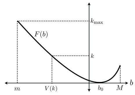
Figure 1: Lemma 1 relates problem (10) to the information theoretic problem (12): $F(V(k))=k$.

Remark 1.

The assumption on $k$ is not restrictive, for if $k=0$ or $k\geq{k_{\rm max}}>0$ then $V(k)$ trivially equals $b_{0}$ or $m$.

Remark 2.

By [5, Theorem 2], the standing assumption (13) is equivalent to (24) below (which automatically holds if $m>-\infty$), and that condition implies $F(b)>0$ for each $b<b_{0}$. In particular, the continuous convex function $F(b),\;b\in(m,b_{0}]$ is strictly decreasing, and $V(k),\;k\in[0,{k_{\rm max}})$ equals its inverse function.

2.2 Basic concepts and facts

Lemma 1 admits to treat Problem (10) using known results about minimising convex integral functionals under moment constraints, specifically with moment mapping defined by $\phi(r):=(1,X(r))$. We will rely upon results in Csiszár and Matúš [8], specified for this moment mapping. Then the value function in [8] becomes

$$J(a,b):=\inf_{p:\int pd\mu=a,\int Xpd\mu=b}H(p),$$ (14)

thus $F(b)=J(1,b)$.

The function $J$ in (14) is convex, and its effective domain ${\rm dom}\,J:=\{(a,b):J(a,b)<+\infty\}$ has interior

$${\mbox{int\;dom\;}}J=\{(a,b):a>0,\,am<b<aM\},$$ (15)

by [8, Lemma 6.6]. The function $J$ is proper (not identically $+\infty$ and never equal to $-\infty$) because it equals zero at $(1,b_{0})\in{\mbox{int\;dom\;}}J$, see (6), (7). Hence its convex conjugate $J^{*}(\theta_{1},\theta_{2}):=\sup_{a,b}[\theta_{1}a+\theta_{2}b-J(a,b)]$ is a closed (i.e., lower semicontinuous) proper convex function. A crucial fact is the instance of [8, Theorem 1.1] that

$$J^{*}({{\theta_{1},\theta_{2}}})=K(\theta_{1},\theta_{2}):=\int\beta^{*}(r,\theta_{1}+\theta_{2}X(r))\mu(dr),$$ (16)

where $\beta^{*}$ is the convex conjugate of $\beta$,

$$\beta^{*}(r,\tau):=\sup_{s\in\mathbb{R}}\left(s\tau-\beta(r,s)\right).$$ (17)

The conjugate and derivatives of $\beta$ are by the second variable.

Below, derivatives at $0$ and $+\infty$ are interpreted as limits of derivatives at $s\downarrow 0$ and $s\uparrow+\infty$. For fixed $r\in\Omega$ the function $\beta^{*}$ equals $-\beta(r,0)$ for $\tau\leq\beta^{\prime}(r,0)$, it is strictly convex in the interval $(\beta^{\prime}(r,0),\beta^{\prime}(r,+\infty))$, and equals $+\infty$ if $\beta^{\prime}(r,+\infty)$ is finite and $\tau>\beta^{\prime}(r,+\infty)$. This function is differentiable in the interval $(-\infty,\beta^{\prime}(r,+\infty))$. Its dervative $(\beta^{*})^{\prime}(r,\tau)$ is positive and strictly increasing in $(\beta^{\prime}(r,0),\beta^{\prime}(r,+\infty))$, and approaches $0$ or $+\infty$ as $\tau\downarrow\beta^{\prime}(r,0)$ or $\tau\uparrow\beta^{\prime}(r,+\infty)$.

Since $J^{*}=K$ implies $J^{**}=K^{*}$, and $J^{**}$ (equal to the closure of $J$) may differ from $J$ only on the boundary of ${\rm dom}\,J$,

$$F(b)=J(1,b)=K^{*}(1,b)=\sup_{{{\theta_{1},\theta_{2}}}}[\theta_{1}+\theta_{2}b-K({{\theta_{1},\theta_{2}}})],$$ (18)

except possibly for $b$ equal to $m$ or $M$, see (15). This can be rewritten as

$$F(b)=\sup_{\theta_{2}}\;[\theta_{2}b-G(\theta_{2})]=G^{*}(b)$$ (19)

where

$$G(\theta_{2}):=\inf_{\theta_{1}}\;[K({{\theta_{1},\theta_{2}}})-\theta_{1}].$$ (20)

The function $G$ will play a similar role as the logarithmic moment generating function does when $\Gamma$ in (3) is an $I$-divergence ball, see Example 3. A consequence of (19) applied to $b=b_{0}$: is the simple bound

$$G(\theta_{2})\geq\theta_{2}b_{0}.$$ (21)

The following family of non-negative functions on $\Omega$ will play a key role like exponential families do for $I$-divergence minimisation:

$$p_{\theta_{1},\theta_{2}}(r):=(\beta^{*})^{\prime}(r,\theta_{1}+\theta_{2}X(r)),\>\>\>(\theta_{1},\theta_{2})\in\Theta$$ (22)

where

$$\Theta:=\left\{(\theta_{1},\theta_{2})\in{\rm dom}\;K:\theta_{1}+\theta_{2}X(r)<\beta^{\prime}(r,+\infty)\quad\mu\mbox{-a.e.}\right\}.$$ (23)

Remark 3.

It may happen that different parameters $({{\theta_{1},\theta_{2}}})\in\Theta$ give rise to equal functions (22), but only in case of functions that equal zero except for $r$ in a set where $X(r)$ is constant $\mu$-a.e. This follows because for any fixed $r\in\Omega$, the fact that $(\beta^{*})^{\prime}(r,\tau)$ is strictly increasing for $\tau\in(\beta^{\prime}(r,0),\beta^{\prime}(r,+\infty))$ implies that $p_{{\theta_{1},\theta_{2}}}(r)$ in (22), if positive, uniquely determines $\theta_{1}+\theta_{2}X(r)$. In particular, for positive valued functions (22) the parameters $({{\theta_{1},\theta_{2}}})\in\Theta$ are always unique, due to the standing assumption (6).

As $({{\theta_{1},\theta_{2}}})\in{\rm dom}\,K$ implies $({{{\tilde{\theta}}_{1},\theta_{2}}})\in\Theta$ for each ${\tilde{\theta}}_{1}<\theta_{1}$, the sets ${\rm dom}\;K$ and $\Theta$ have the same projection to the $\theta_{2}$-axis. This projection will be denoted by $\Theta_{2}$. It is a (finite or infinite) interval. The standing assumptions (6), (7) imply that $\Theta_{2}$ contains the origin, and the default density $p_{0}$ belongs to the family (22) with $\theta_{2}=0$, see [5, Remark 4]. The left endpoint of the interval $\Theta_{2}$ will be denoted by $\theta_{\min}$. By [5, Theorem 2], the standing assumption ${k_{\rm max}}>0$ is equivalent to

$$\theta_{\min}<0.$$ (24)

By [8, Lemma 3.6], the directional derivatives of the function $K$ in (16) can be expressed, at any $({{\theta_{1},\theta_{2}}})\in\Theta$ and for any $({\tilde{\theta}}_{1},{\tilde{\theta}}_{2})\in{\rm dom}\,K$, as

$$\lim_{t\downarrow 0}\frac{1}{t}\left[K(\theta_{1}+t({\tilde{\theta}}_{1}-\theta_{1}),\theta_{2}+t({\tilde{\theta}}_{2}-\theta_{2}))-K({{\theta_{1},\theta_{2}}})\right]$$

$$=\int\left[{\tilde{\theta}}_{1}-\theta_{1}+({\tilde{\theta}}_{2}-\theta_{2})X(r)\right]{p_{\theta_{1},\theta_{2}}}(r)\mu(dr),$$ (25)

where the integral is well-defined and is not equal to $+\infty$. In particular, $K$ is differentiable in the interior of its effective domain, with

$$\frac{\partial}{\partial\theta_{1}}K({{\theta_{1},\theta_{2}}}) = \int p_{\theta_{1},\theta_{2}}d\mu,$$ (26)

$$\frac{\partial}{\partial\theta_{2}}K({{\theta_{1},\theta_{2}}}) = \int Xp_{\theta_{1},\theta_{2}}d\mu.$$ (27)

The same equations hold at $({{\theta_{1},\theta_{2}}})\in\Theta$ on the boundary of ${\rm dom}\,K$ for those one-sided partial derivatives of $K$ which are defined there, thus (26) holds for the left partial derivative at each $({{\theta_{1},\theta_{2}}})\in\Theta$.

The following lemma gives relevant information about evaluating the function $G$ in (20). Its proof is effectively contained in the proof of [5, Proposition 2], but for convenience a full proof will be given in the Appendix. Clearly, ${\rm dom}\,G:=\{\theta_{2}:G(\theta_{2})<+\infty\}=\Theta_{2}.$

Lemma 2.

Given any $\theta_{2}\in\Theta_{2}$, either (i) some $\bar{\theta}_{1}\in\mathbb{R}$ satisfies $(\bar{\theta}_{1},\theta_{2})\in\Theta$, $\int p_{\bar{\theta}_{1},\theta_{2}}d\mu=1$, or (ii) ${\tilde{\theta}}_{1}:=\sup\{\theta_{1}:({{\theta_{1},\theta_{2}}})\in{\rm dom}\,K\}$ is finite, $({\tilde{\theta}}_{1},\theta_{2})\in\Theta$, $\int p_{{\tilde{\theta}}_{1},\theta_{2}}d\mu<1$. In either case, in (20) the minimum is attained, and the unique minimiser is $\bar{\theta}_{1}$ respectively ${\tilde{\theta}}_{1}$.

2.3 Generalised Pythagorean identity

Given the convex integrand $\beta$, define $\Delta_{\beta(r,\cdot)}(s,t)$ as in (8), with the convex function $\beta(r,\cdot):s\mapsto\beta(r,s)$ playing the role of $f$. The mapping $(r,s,t)\mapsto\Delta_{\beta(r,\cdot)}(s,t)$ is a normal integrand [8, Lemma 2.10], hence if $p$ and $q$ are non-negative measurable functions on $\Omega$ then so is also $\Delta_{\beta(r,\cdot)}(p(r),q(r))$, denoted briefly by $\Delta_{\beta}(p,q)$. Extending the concept of Bregman distance (9), define

$$B(p,q)=B_{\beta,\mu}(p,q):=\int\Delta_{\beta}(p,q)d\mu.$$ (28)

Like its special case in (9), it is non-negative and equals $0$ only if $p=q$. If $\beta=\Delta_{f}$, as in Example 2, then $B_{\beta,\mu}$ is equal to the $B_{f,\mu}$ of (9).

The following lemma, crucial for this paper, is an instance of [8, Lemma 4.15], combined with [8, Remark 4.13]

Lemma 3.

For each density $p$ with $\int Xpd\mu$ finite, and each $({{\theta_{1},\theta_{2}}})\in\Theta$,

$$H(p)=\theta_{1}+\theta_{2}\int Xpd\mu-K({{\theta_{1},\theta_{2}}})+B(p,p_{{\theta_{1},\theta_{2}}})$$

$$+\int|\beta^{\prime}(r,0)-\theta_{1}-\theta_{2}X(r)|_{+}p(r)\mu(dr).$$ (29)

If $p_{{\theta_{1},\theta_{2}}}$ is a density, the special case $p=p_{{\theta_{1},\theta_{2}}}$ of (3) (or direct calculation) gives that

$$H(p_{{\theta_{1},\theta_{2}}})=\theta_{1}+\theta_{2}\int Xp_{{\theta_{1},\theta_{2}}}d\mu-K({{\theta_{1},\theta_{2}}}).$$ (30)

Then (3) and (30) imply

$$H(p)=H(p_{{\theta_{1},\theta_{2}}})+B(p,p_{{\theta_{1},\theta_{2}}})+\int|\beta^{\prime}(r,0)-\theta_{1}-\theta_{2}X(r)|_{+}p(r)\mu(dr)$$ (31)

for each density $p$ satisfying

$$\int Xpd\mu=\int Xp_{{\theta_{1},\theta_{2}}}d\mu.$$ (32)

Identities like (31) frequently occur in the literature, primarily in cases when the last term vanishes (it trivially does if $\beta^{\prime}(r,0)=-\infty$). They are referred to as Pythagorean identities, and (3) will be called generalised Pythagorean identity.

The above results admit a short proof of the following key lemma, see [5, Theorem 1] for a related result.

Lemma 4.

(i) Let $({{\theta_{1},\theta_{2}}})\in\Theta$, $\int p_{{\theta_{1},\theta_{2}}}d\mu=1$. Then $\int Xp_{{\theta_{1},\theta_{2}}}d\mu$ is finite if and only if $H(p_{{\theta_{1},\theta_{2}}})$ is. In that case the density $p=p_{{\theta_{1},\theta_{2}}}$ uniquely attains the minimum in the definition (12) of $F(b)$ for $b:=\int Xp_{{\theta_{1},\theta_{2}}}d\mu$, and

$$F(b)=H(p_{{\theta_{1},\theta_{2}}})=\theta_{1}+\theta_{2}b-K({{\theta_{1},\theta_{2}}})=\theta_{2}b-G(\theta_{2}).$$ (33)

Supposing $H(p_{{\theta_{1},\theta_{2}}})>0$, here $b$ is less or larger than $b_{0}$ according as $\theta_{2}$ is negative or positive.

(ii) For $k\in(0,{k_{\rm max}})$, a density $p$ attains the minimum in the definition (10) of $V(k)$ if and only if $p=p_{{\theta_{1},\theta_{2}}}$ for some $({{\theta_{1},\theta_{2}}})\in\Theta$ with $\theta_{2}<0$ and

$$H(p_{{\theta_{1},\theta_{2}}})=k\quad\mbox{or equivalently}\quad\int Xp_{{\theta_{1},\theta_{2}}}d\mu=V(k).$$ (34)

Proof.

The first assertion holds by (30), and the second one since (31), (32) imply $H(p)>H(p_{{\theta_{1},\theta_{2}}})$ for each density $p$ with $\int Xpd\mu=b=\int Xp_{{\theta_{1},\theta_{2}}}d\mu$. Then (33) follows by (30) and the consequence $K({{\theta_{1},\theta_{2}}})-\theta_{1}=G(\theta_{2})$ of Lemma 2. Finally, (21) and (33) yield $\theta_{2}b>\theta_{2}b_{0}$, proving the last assertion of part (i).

(ii) For sufficiency, it is enough to verify the equivalence (34), under the given hypotheses. The function $V:(0,{k_{\rm max}})\rightarrow(m,b_{0})$ is the inverse of $F:(m,b_{0})\rightarrow(0,{k_{\rm max}})$, see Lemma 1 and Remark 2. This and the result $F(\int Xp_{{\theta_{1},\theta_{2}}}d\mu)=H(p_{{\theta_{1},\theta_{2}}})$ of part (i) imply (34), because if $0<H(p_{{\theta_{1},\theta_{2}}})<{k_{\rm max}}$ then $m<\int Xp_{{\theta_{1},\theta_{2}}}d\mu<b_{0}$ (the upper bound follows from $\theta_{2}<0$, due to the last assertion of part (i)). Regarding necessity, a density $p$ that attains the minimum in (10) clearly satisfies the constraint $H(p)\leq k$ with the equality. We skip the proof of the remaining assertion that $p$ has to be of form $p_{{\theta_{1},\theta_{2}}}$ with $\theta_{2}<0$, for this will be an immediate consequence of Theorem 2. ∎

3 New results

3.1 Calculating V(k)

A procedure to calculate $V(k)$ in (10) is to first determine the function $K$ in (16), then the function $F$ via (18) (this may be done in two steps, first determining the function $G$ in (20)), and finally $V(k)$ as the solution $b\in(m,b_{0})$ of the equation $F(b)=k$, see Lemma 1. In regular cases, $b=V(k)$ is characterised by equations involving partial derivatives of the function $K$, see [5, Corollary 1], which may facilitate its computation. The following Theorem, combined with Lemma 2, may help to reduce computational complexity even in “irregular”cases. Previously, Ahmadi-Javid [1, Theorem 5.1] proved an identity equivalent to (35) for autonomous integrands and bounded payoff functions.

A lemma is sent forward that will be proved in the Appendix.

Lemma 5.

$F^{*}=G$.

Note that while $F^{*}=G^{**}={\rm cl}{G}$ immediately follows from (19), it appears nontrivial that the function $G$ is closed.

Theorem 1.

For $k\in(0,{k_{\rm max}})$

$$V(k)=\max_{\theta_{2}<0}\max_{\theta_{1}\in\mathbb{R}}\frac{k+K({{\theta_{1},\theta_{2}}})-\theta_{1}}{\theta_{2}}=\max_{\theta_{2}<0}\frac{k+G(\theta_{2})}{\theta_{2}}.$$ (35)

A maximiser for the second maximum in (35) is equivalently a maximiser of $\theta_{2}b-G(\theta_{2})$ where $b=V(k)$. A pair $({{\theta_{1},\theta_{2}}})$ attains the first maximum in (35) if and only if it attains the maximum in (18), for $b=V(k)$. Such $({{\theta_{1},\theta_{2}}})$ belongs to $\Theta$ and satisfies $\int p_{{\theta_{1},\theta_{2}}}d\mu\leq 1$.

Proof.

The conditions $b=V(k)$, $k\in(0,{k_{\rm max}})$ are equivalent to $F(b)=k$, $b\in(m,b_{0})$, see Lemma 1 and Remark 2. The condition that $\theta_{2}$ is a maximiser of $\theta_{2}b-G(\theta_{2})$ means, by (19), that

$$\theta_{2}b-G(\theta_{2})=G^{*}(b)=F(b)=k$$ (36)

or equivalently, see Lemma 5, that $\theta_{2}b-F(b)=F^{*}(\theta_{2})$. This proves that $\theta_{2}$ is a maximiser of $\theta_{2}b-G(\theta_{2})$ if and only if $F^{\prime}_{-}(b)\leq\theta_{2}\leq F^{\prime}_{+}(b)$. In particular, a (perhaps non-unique) maximiser $\theta_{2}<0$ does exist.

By (36), the maximum of $\theta_{2}b-G(\theta_{2})$ equals $k$, hence $\theta_{2}b-G(\theta_{2})\leq k$ for each $\theta_{2}\in\mathbb{R}$. This proves the assertions that the maximum of

$$\frac{k+G(\theta_{2})}{\theta_{2}}\quad\quad(\theta_{2}<0)$$ (37)

is equal to $b=V(k)$, and a maximiser of (37) is equivalently a maximiser of $\theta_{2}b-G(\theta_{2})$. The remaining assertions of Theorem 1 immediately follow from this and Lemma 2. ∎

The calculation of $W(\lambda)$ in (11) is somewhat less costly than that of $V(k)$. It requires the calculation of $G(\theta_{2})$ only for a single value of $\theta_{2}$, since for $\lambda>0$ we have (using Lemma 5 in the final step)

$$W(\lambda)=\inf_{b}[b+\lambda F(b)]=-\lambda\sup_{b}[-\frac{b}{\lambda}-F(b)]$$

$$=-\lambda F^{*}(-\frac{1}{\lambda})=-\lambda G(-\frac{1}{\lambda}).$$ (38)

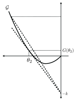
Figure 2: The supporting line has maximum slope $b=(k+G(\theta_{2}))/\theta_{2}$ among all lines passing through $(0,-k)$ and some point of $\mathcal{G}$. This slope is equal to the solution $V(k)$ of problem (10).

Remark 4.

The following geometric interpretation of the proof of Theorem 1 deserves emphasis, see Fig. 2. Denote by

$$\mathcal{G}:=\{(\theta_{2},G(\theta_{2})):\theta_{2}\in\Theta_{2},\>\theta_{2}\leq 0\}$$ (39)

the graph of $G$ restricted to nonpositive arguments. Recall that, by Lemma 5, $G$ is a closed convex function with $G(0)=0$. Then (37) is the slope of the straight line through $(0,-k)$ and $(\theta_{2},G(\theta_{2}))\in\mathcal{G}$, which is maximised by the supporting line to $\mathcal{G}$ through $(0,-k)$. The proof of Theorem 1 shows that this supporting line (exists and) has slope $b=V(k)$. The maximum $b=V(k)$ of (37) is attained if and only if $(\theta_{2},G(\theta_{2}))$ is on this supporting line.

3.2 Almost worst case distributions

For the problem (10), call a density $p$ an $(\epsilon$-$\gamma)$-Almost-Worst-Case-Density (AWCD), where $\epsilon\geq 0,\;\gamma\geq 0$, if

$$H(p)\leq k+\gamma\quad\mbox{and}\quad\int Xpd\mu\leq V(k)+\epsilon.$$ (40)

Thus, an $(\epsilon$-$\gamma)$-AWCD is a density which does not violate the constraint $H(p)\leq k$ by more than $\gamma$ and for which the expected payoff does not exceed by more than $\epsilon$ the worst possible one subject to the constraint. A worst case density (WCD) is a $(0$-$0)$-AWCD.

An $(\epsilon$-$\gamma)$ almost worst case distribution or a worst case distribution is a distribution ${\mathbb{P}}$ whose density is an $(\epsilon$-$\gamma)$-AWCD or a WCD.

Theorem 2 below establishes a clustering property of the $(\epsilon$-$\gamma)$-AWCDs, as well as a similar result for densities that almost attain the minimum in (11). From a practical point of view, this may be relevant for efficient hedging against the almost worst scenarios, but this issue is not entered here.

Let us assign to each $\theta_{2}\in\Theta_{2}$ the unique $\theta_{1}$ attaining the minimum in the definition (20) of $G(\theta_{2})$, determined in Lemma 2, and denote

$${q_{\theta_{2}}}(r):=p_{{\theta_{1},\theta_{2}}}(r),\;\mbox{with $\theta_{1}$ attaining}\;K({{\theta_{1},\theta_{2}}})-\theta_{1}=G(\theta_{2}).$$ (41)

Given $k\in(0,{k_{\rm max}})$, we will denote by ${\hat{q}_{k}}$ the function ${q_{\theta_{2}}}$ with $\theta_{2}<0$ attaining the second maximum in Theorem 1, i.e.,

$${\hat{q}_{k}}:={q_{\theta_{2}}}=p_{{\theta_{1},\theta_{2}}}\quad\mbox{with $({{\theta_{1},\theta_{2}}})$ a maximiser in~{}\eqref{mm}}$$ (42)

Theorem 2.

(i) For $k\in(0,{k_{\rm max}})$, each $(\epsilon$-$\gamma)$-AWCD $p$ belongs to the
Bregman neighborhood of radius $(\gamma-\theta_{2}\epsilon)$ of ${\hat{q}_{k}}$ in (42), i.e., see (28),

$$B(p,{\hat{q}_{k}})\leq\gamma-\theta_{2}\epsilon\quad\mbox{if $p$ is an $(\epsilon$-$\gamma)$-AWCD}.$$ (43)

(ii) For $\lambda>0$ with $-1/\lambda\in\Theta_{2}$, set $\theta_{2}:=-1/\lambda$. Then for each density $p$

$$\int Xpd\mu+\lambda H(p)\geq W(\lambda)+\lambda B(p,{q_{\theta_{2}}}).$$ (44)

Corollary 1.

Let $\{p_{n}\}$ be a sequence of $(\epsilon_{n}$-$\gamma_{n})$-AWCDs with $\epsilon_{n}\to 0,\;\gamma_{n}\to 0$ in case (i), or a sequence of densities with $\int Xp_{n}d\mu+\lambda H(p_{n})\to W(\lambda)$ in case (ii). Then $p_{n}$ converges to ${\hat{q}_{k}}$ respectively to ${q_{\theta_{2}}}$ locally in measure. In particular, the function ${\hat{q}_{k}}$ is unique.

Proof.

(i) By the generalised Pythagorean identity Lemma 3, applied to ${{\theta_{1},\theta_{2}}}$ in (42),

$$H(p)\geq\theta_{1}+\theta_{2}\int Xpd\mu-K({{\theta_{1},\theta_{2}}})+B(p,p_{{\theta_{1},\theta_{2}}})$$

$$=\theta_{2}\int Xpd\mu-G(\theta_{2})+B(p,{q_{\theta_{2}}}),$$ (45)

for each density $p$. As $\theta_{2}$ attains the maximum in Theorem 1, here ${q_{\theta_{2}}}={\hat{q}_{k}}$ and $G(\theta_{2})=\theta_{2}V(k)-k$. Hence, (3.2) implies (43) for each density $p$ which is an $(\epsilon$-$\gamma)$-AWCD, thus satisfies (40).

(ii) In this case, (3.2) holds as before. Multiplying it by $\lambda=-1/\theta_{2}$ and using that $-\lambda G(-1/\lambda)=W(\lambda)$, see (3.1), we obtain (44).

The Corollary follows since $B(p_{n},{\hat{q}_{k}})\to 0$ implies convergence of $p_{n}$ to ${q_{\theta_{2}}}$ locally in measure [8, Corollary 2.14]. ∎

Remark 5.

Corollary 1 extends the known result that ${\hat{q}_{k}}$ is a generalized solution of problem (12) in the sense [8] that densities $p_{n}$ with $\int Xp_{n}d\mu=b=V(k),\;H(p_{n})\to F(b)=k$ converge to ${\hat{q}_{k}}$ locally in measure, and also establishes its (new) counterpart for problem (10).

The function ${\hat{q}_{k}}$ in Theorem 2(i) will be called worst case localiser, for the almost worst case densities are clustering in its (Bregman) neighborhood. This nice intuitive interpretation of the function ${\hat{q}_{k}}=p_{{\theta_{1},\theta_{2}}}$ is complemented by the additional intuitive fact that, by (43), its parameter $\theta_{2}$ controls the radius of that neighborhood. Most appealing is the special case $\gamma=0$ of (43) that all densities that satisfy $H(p)\leq k$ and yield expected payoff not excceding the worst case by more than $\epsilon$, are contained in a Bregman neighborhood of ${\hat{q}_{k}}$ of radius proportional to $\epsilon$, with proportionality factor $-\theta_{2}$. The essence of the Corollary is that the Bregman distance of $p_{n}$ from ${\hat{q}_{k}}$ goes to $0$. For certain choices of the integrand $\beta$ this implies convergence even in a stronger sense than locally in measure, see Example 3.

Clearly, the worst case localiser ${\hat{q}_{k}}$ coincides with the WCD whenever the latter exists (apply (43) to $\epsilon=\gamma=0$). A necessary and sufficient condition for the existence of a WCD is given in Lemma 4(ii). There, we have skipped the proof that a WCD has to be of form $p_{{\theta_{1},\theta_{2}}}$ with $\theta_{2}<0$, which is obvious now as the WCD is a worst case localiser. Lemma 6 below will also be useful in identifying situations when the worst case localiser is actually a WCD. Its Corollary addresses the simplest such situation. When in (10) the minimum is not attained, the worst case localiser may or may not be a density, see the examples below, though it always satisfies $\int{\hat{q}_{k}}d\mu\leq 1$, see Theorem 1. Note that the computation of the worst case localiser is not harder than the computation of $V(k)$ along the lines of Subsection 3.1, for that calculation does provide the parameters ${{\theta_{1},\theta_{2}}}$ of ${\hat{q}_{k}}=p_{{\theta_{1},\theta_{2}}}$ that attain the double maximum in Theorem 1.

Lemma 6.

A function $p_{{\theta_{1},\theta_{2}}}$ in (22) with $\theta_{2}<0$ is the worst case localiser ${\hat{q}_{k}}$ for $k\in(0,{k_{\rm max}})$ if and only if the vector $(1-\int p_{{\theta_{1},\theta_{2}}}d\mu,\,V(k)-\int Xp_{{\theta_{1},\theta_{2}}}d\mu)\in\mathbb{R}^{2}$ belongs to the normal cone of ${\rm dom}\,K$ at $({{\theta_{1},\theta_{2}}})$, i.e., for each $({{{\overline{\theta}}_{1},{\overline{\theta}}_{2}}})\in{\rm dom}\,K$

$$(\bar{\theta}_{1}-\theta_{1})\left(1-\int p_{{\theta_{1},\theta_{2}}}d\mu\right)+(\bar{\theta}_{2}-\theta_{2})\left(V(k)-\int Xp_{{\theta_{1},\theta_{2}}}d\mu\right)\leq 0.$$ (46)

Corollary 2.

If the worst case localiser ${\hat{q}_{k}}=p_{{\theta_{1},\theta_{2}}}$ has parameters $({{\theta_{1},\theta_{2}}})$ in the interior of ${\rm dom}\,K$, then it is a WCD.

Proof.

By Theorem 1, the condition in the definition (42) is equivalent to the condition that $({{\theta_{1},\theta_{2}}})$ attains the maximum of $f({{\theta_{1},\theta_{2}}}):=\theta_{1}+\theta_{2}b-K({{\theta_{1},\theta_{2}}})$ where $b=V(k)$. The latter is satisfied if and only if for each $({{{\overline{\theta}}_{1},{\overline{\theta}}_{2}}})\in{\rm dom}\,K$, the concave function

$$f(t):=f(\theta_{1}+t(\bar{\theta}_{1}-\theta_{1}),\;\theta_{2}+t(\bar{\theta}_{2}-\theta_{2})),\quad 0\leq t\leq 1$$

is maximised by $t=0$, i.e., its (right) derivative at $t=0$ is nonpositive. On account of (2.2), that condition is equivalent to (46). The Corollary follows since the normal cone of ${\rm dom}\,K$ at an interior point consists of $(0,0)$ alone. Thus Lemma 6 gives the conditions $\int p_{{\theta_{1},\theta_{2}}}d\mu=1,\int Xp_{{\theta_{1},\theta_{2}}}d\mu=V(k)$, which mean by Lemma 4 that $p_{{\theta_{1},\theta_{2}}}$ is a WCD. ∎

Example 3.

Let $H(p)$ be the $I$-divergence, formally (see Example 1) let $\beta$ be the autonomous integrand given by $f(s)=s\log s$ and let ${\mathbb{P}}_{0}=\mu$. Then $f^{*}(\tau)=e^{\tau-1}$, $K({{\theta_{1},\theta_{2}}})=\int e^{\theta_{1}+\theta_{2}X-1}d\mu$, and

$$G(\theta_{2})=\min_{\theta_{1}}[K({{\theta_{1},\theta_{2}}})-\theta_{1}]=\log\int e^{\theta_{2}X}d\mu:=\Lambda(\theta_{2}),$$

for $\theta_{2}\in\Theta_{2}={\rm dom}\>\Lambda$. The minimum in the definition of $G(\theta_{2})$ is attained for $\theta_{1}=1-\Lambda(\theta_{2})$. If $m>-\infty$ and $X(r)=m$ on a set of $\mu$-measure $\mu_{0}>0$ then ${k_{\rm max}}=-\log\mu_{0}$, otherwise ${k_{\rm max}}=+\infty$ (assuming (24)).

For $k\in(0,{k_{\rm max}})$, Theorem 1 gives $V(k)=\max_{\theta_{2}<0}[k+\Lambda(\theta_{2})]/\theta_{2}$ and Theorem 2 gives the worst case localiser ${\hat{q}_{k}}=\exp(-\Lambda(\theta_{2})+\theta_{2}X)$, with $\theta_{2}$ attaining the above maximum. This worst case localiser is always a density. It also satisfies $H({\hat{q}_{k}})=k$ and hence is actually a WCD, except for the case when ${\rm dom}\,\Lambda$ contains its left endpoint ${\theta_{\rm min}}$, $\Lambda^{\prime}({\theta_{\rm min}})$ is finite, and $k>H(q_{{\theta_{\rm min}}})$. In that case the maximiser in Theorem 1, equal to the parameter of the worst case localiser, is $\theta_{2}={\theta_{\rm min}}$. Note that for this example, the formula for $V(k)$ appears in [1] and [5] show that in the above exceptional case the minimum in (10) is not attained. The result of Theorem 2 appears new even for this special case.

In this example, the Bregman distance (28) of densities coincides with $I$-divergence, hence Theorem 2 gives $D(p||{\hat{q}_{k}})\leq\gamma-\theta_{2}\epsilon$ for each $(\epsilon$-$\gamma)$-AWCD $p$. In the Corollary of Theorem 2, now the almost worst case densities converge to the worst case localiser in a much stronger sense than in measure. Indeed, the result that their $I$-divergence from the worst case localiser approaches $0$ is stronger than $L_{1}(\mu)$ convergence to the worst case localiser.

Example 4.

Again in the setting of Example 1, take now $f(s)=-\log s$. Then $H(p)$ equals reverse $I$-divergence, i.e., the $I$-divergence of the default distribution ${\mathbb{P}}_{0}=\mu$ from the distribution ${\mathbb{P}}$ with density $p$. As $f$ is not cofinite, the standing assumption ${k_{\rm max}}>0$ holds if and only if $m>-\infty$.

Take specifically $\Omega=(0,1),\;X(r)=r$, and take for $\mu={\mathbb{P}}_{0}$ the distribution with Lebesgue density $2r$. As $f^{*}(\tau)=-1-\log(-\tau)\;(\tau<0)$, then $K({{\theta_{1},\theta_{2}}})=\int_{0}^{1}[-1-\log(-\theta_{1}-\theta_{2}r)]\,2rdr$ and $p_{{\theta_{1},\theta_{2}}}(r)=1/(-\theta_{1}-\theta_{2}r)$ for $({{\theta_{1},\theta_{2}}})\in\Theta={\rm dom}\,K=\{({{\theta_{1},\theta_{2}}}):\theta_{1}\leq 0,\,\theta_{1}+\theta_{2}<0\}$. Simple calculus shows that for $-2\leq\theta_{2}\leq 0$ the minimum in the definition of $G(\theta_{2})$ is attained for $\theta_{1}$ such that $p_{{\theta_{1},\theta_{2}}}={q_{\theta_{2}}}$ is a density, but the functions $G$ and ${q_{\theta_{2}}}$ can not be given explicitly. If $\theta_{2}<-2$ then this minimum is attained for $\theta_{1}=0$, and $G(\theta_{2})=-\frac{1}{2}-\log(-\theta_{2})$. One sees that $H({q_{\theta_{2}}})$ ranges from $0$ to $\log 2-1/2$ as $\theta_{2}$ ranges from $0$ to $-2$. Hence in case $k\leq\log 2-1/2$ the WCD exists, it equals that $p_{{\theta_{1},\theta_{2}}}$ which is a density and satisfies $H(p_{{\theta_{1},\theta_{2}}})=k$. In case $k\geq\log 2-1/2$ the worst case localiser is ${\hat{q}_{k}}(r)=-1/\theta_{2}r$ with $\theta_{2}\leq-2$ attaining $V(k)=\max_{\theta_{2}<0}[k+G(\theta_{2})]/\theta_{2}$. By simple calculus, this maximiser is $\theta_{2}=-e^{k+1/2}$, the maximum is $V(k)=e^{-(k+1/2)}$, and the worst case localiser is ${\hat{q}_{k}}(r)=\frac{1}{r}e^{-(k+1/2)}$, which is not a density unless $k=\log 2-1/2$.

In this case the Bregman distance (28) is

$$B(p,q)=\int\left[\log\frac{q}{p}+\frac{p}{q}-1\right]d\mu.$$

The Corollary of Theorem 2 now does not admit a substantial strengthening, for the result that this Bregman distance approaches $0$ does not imply convergence in a familiar sense stronger than in measure.

Example 5.

Let $\Omega,\;X,\;\mu$ be as in Example 4, but this time let the default distribution ${\mathbb{P}}_{0}$ be the uniform distribution whose $\mu$-density is $p_{0}(r)=\frac{1}{2r}$. Take for $H(p)$ the Bregman distance $B(p,p_{0})$ in Example 4, i.e., the integral functional (4) with $\beta(r,s)=\Delta_{f}(s,p_{0}(r))=-\log s-\log(2r)+2r(s-\frac{1}{2r})$. Then $\beta^{*}(r,\tau)=\log{2r}-\log(-\tau+2r)$, $(\beta^{*})^{\prime}(r,s)=1/(-\tau+2r)$, $\tau<2r$. The set $\Theta$ (equal to ${\rm dom}\,K$) of this example consists of those $({{\theta_{1},\theta_{2}}})$ for which $(\theta_{1},\theta_{2}-\theta_{1})$ belongs to the set $\Theta={\rm dom}\,K$ of Example 4. Moreover, for such $({{\theta_{1},\theta_{2}}})$ the function $p_{{\theta_{1},\theta_{2}}}(r)=1/[-\theta_{1}-(\theta_{2}-2)r]$ coincides with the function $p_{\theta_{1},\theta_{2}-2}$ of Example 4, which can not be a density if $\theta_{2}<0$. This proves that in the present Example no WCD exists for any $k>0$.

3.3 Effect of the threshold $k$ on the existence of a WCD

This subsection addresses the effect of the choice of the threshold $k$ on the worst case localiser, in particular on whether that localiser is also a WCD.

Examples 3, 4, and 5 demonstrate that a WCD may exist for all or for no $k$, or there may exist a critical value ${k_{\rm cr}}$ such that a WCD exists if $k<{k_{\rm cr}}$ but does not exist if $k>{k_{\rm cr}}$. It appears a plausible conjecture that these three alternatives are exhaustive, i.e., that if a WCD exists for some $k$, it also exists for each $k^{\prime}<k$. While this conjecture remains open in general, it will be proved under conditions that cover many typical cases.

Recall that ${\theta_{\rm min}}$ with $-\infty\leq{\theta_{\rm min}}<0$ denotes the left endpoint of the interval $\Theta_{2}$, the projection of ${\rm dom}\,K$ to the $\theta_{2}$ axis. The condition $m>-\infty$ is necessary for ${k_{\rm max}}<+\infty$ and sufficient for ${\theta_{\rm min}}=-\infty$.

Theorem 3.

(i) If for some $k\in(0,{k_{\rm max}})$ the worst case localiser ${\hat{q}_{k}}$ is a density, it is a WCD for $k$ unless

$${\theta_{\rm min}}\in\Theta_{2},\quad G^{\prime}({\theta_{\rm min}})>-\infty$$ (47)

and

$$k>{k_{\rm cr}}:=-G({\theta_{\rm min}})+{\theta_{\rm min}}G^{\prime}({\theta_{\rm min}}).$$ (48)

If (47) and (48) hold then ${\hat{q}_{k}}=\hat{q}_{{k_{\rm cr}}}=q_{{\theta_{\rm min}}}$ and no WCD exists for $k$.

(ii) If ${\rm dom}\,K$ contains the $\theta_{1}$-axis, i.e., $\int\beta^{*}(r,\theta_{1})\mu(dr)$ is finite for each $\theta_{1}\in\mathbb{R}$, then the worst case localiser ${\hat{q}_{k}}$ is a density and hence it is a WCD unless (47) and (48) hold.

Proof.

(i) Suppose ${\hat{q}_{k}}=p_{{\theta_{1},\theta_{2}}}$ in (42) is a density. By Lemma 4 it is a WCD for $k$ if and only if

$$\int Xp_{{\theta_{1},\theta_{2}}}d\mu=V(k).$$ (49)

Since $p_{{\theta_{1},\theta_{2}}}$ is a worst case localiser and $\int p_{{\theta_{1},\theta_{2}}}=1$, Lemma 6 gives that

$$(\bar{\theta}_{2}-\theta_{2})\left(V(k)-\int Xp_{{\theta_{1},\theta_{2}}}d\mu\right)\leq 0\quad\mbox{for}\quad\bar{\theta}_{2}\in\Theta_{2}.$$ (50)

This immediately implies  (49) if $\theta_{2}\neq{\theta_{\rm min}}$, or equivalently (see Remark 4) if the supporting line through $(0,-k)$ to the curve $\mathcal{G}$ does not contain $({\theta_{\rm min}},G({\theta_{\rm min}}))$. This is always the case if (47) does not hold, and also when (47) holds but $G^{\prime}({\theta_{\rm min}})$, the largest slope of supporting lines to $\mathcal{G}$ at $({\theta_{\rm min}},G({\theta_{\rm min}}))$, is less than $[k+G({\theta_{\rm min}})]/{\theta_{\rm min}}$. As the last condition is equivalent to $k<{k_{\rm cr}}$, only the case $k={k_{\rm cr}}$ remains to cover to complete the proof that ${\hat{q}_{k}}$ is a WCD unless (47) and (48) hold.

In that remaining case, ${\hat{q}_{k}}=p_{{\theta_{1},\theta_{2}}}$ with $\theta_{2}={\theta_{\rm min}}$, and instead of (49) only the inequality $\int X{p_{\theta_{1},\theta_{2}}}d\mu\geq V({k_{\rm cr}})$ follows from (50). Suppose indirectly that it is strict, then Lemma 1 implies that $\int X{p_{\theta_{1},\theta_{2}}}d\mu=V(\bar{k})$ for some $\bar{k}\in(0,{k_{\rm cr}})$ (as the integral is less than $b_{0}$ by Lemma 4). This means by Lemma 4 that $p_{{\theta_{1},\theta_{2}}}$ (with $\theta_{2}={\theta_{\rm min}}$) is a WCD for $\bar{k}$. Hence, by Remark 4, the supporting line through $(0,-\bar{k})$ to the curve $\mathcal{G}$ contains $({\theta_{\rm min}},G({\theta_{\rm min}}))$, contradicting the fact that among the supporting lines to $\mathcal{G}$ at $({\theta_{\rm min}},G({\theta_{\rm min}}))$ the one through $(0,-{k_{\rm cr}})$ has the largest slope. This contradiction proves that (49) holds and hence ${\hat{q}_{k}}$ is a WCD also when $k={k_{\rm cr}}$.

The last assertions of part (i) are obvious. Indeed, if (47) holds and $k>{k_{\rm cr}}$ then the supporting line through $(0,-k)$ to $\mathcal{G}$ meets the curve at $({\theta_{\rm min}},G({\theta_{\rm min}}))$, just as the supporting line through $(0,-{k_{\rm cr}})$ does, hence ${\hat{q}_{k}}=q_{{\theta_{\rm min}}}=q_{{k_{\rm cr}}}$. As it is a WCD for ${k_{\rm cr}}$, it can not be a WCD for $k>{k_{\rm cr}}$ with $V(k)<V({k_{\rm cr}})$.

(ii) The hypothesis implies that a vector in $\mathbb{R}^{2}$ can belong to the normal cone of ${\rm dom}\,K$ at some $({{\theta_{1},\theta_{2}}})$ only if the first component of this vector is $0$. On account of Lemma 6, this proves that the worst case localiser ${\hat{q}_{k}}=p_{{\theta_{1},\theta_{2}}}$, for any $k\in(0,{k_{\rm max}})$, has to satisfy $\int p_{{\theta_{1},\theta_{2}}}d\mu=1$. ∎

Corollary 3.

The function $G$ is differentiable at each $\theta_{2}\in({\theta_{\rm min}},0)$ for which ${q_{\theta_{2}}}$ in (41) is a density.

Proof.

Suppose indirectly that the curve $\mathcal{G}$ has several supporting lines at $(\theta_{2},G(\theta_{2}))$, say one containing $(0,-k_{1})$ and another $(0,-k_{2})$, where $k_{1}\neq k_{2}$. Then $\hat{q}_{k_{1}}=\hat{q}_{k_{2}}={q_{\theta_{2}}}$, see Remark 4, hence ${q_{\theta_{2}}}$ is the WCD both for $k_{1}$ and $k_{2}$, by Theorem 3. This means that $V(k_{1})=\int X{q_{\theta_{2}}}d\mu=V(k_{2})$, contradicting $k_{1}\neq k_{2}$. ∎

Finally, we discuss for $f$-divergence balls, see Example 1, the dependence on the threshold $k$ (the “radius” of the ball) of the worst case localiser and whether it is a WCD. Formally, let $\beta(r,s)=f(s)$ be an autonomous integrand, $f$ strictly convex and differentiable on $(0,+\infty)$, $f(0)=\lim_{s\downarrow 0}f(s)$, $f(1)=0$, let $\mu$ be a probability measure, and ${\mathbb{P}}_{0}=\mu$.

The case of cofinite $f$ is covered by Theorem 3(ii), the integral in its hypothesis being equal to $f^{*}(\theta_{1})$, finite for each $\theta_{1}\in\mathbb{R}$. Therefore we focus on the non-cofinite case, supposing

$$\lim_{s\uparrow+\infty}\frac{f(s)}{s}=c,\quad\quad c\quad\mbox{finite}.$$ (51)

Then the standing assumption ${k_{\rm max}}>0$ (equivalent to ${\theta_{\rm min}}<0$) holds if and only if $m>-\infty$. With no loss of generality, assume that $m=0$ (clearly, the minimisation problem (10) is not affected by adding a constant to $X$).

Under the above assumptions, $K({{\theta_{1},\theta_{2}}})=\int f^{*}(\theta_{1}+\theta_{2}X)d\mu$ with $\theta_{2}<0$ is finite if $\theta_{1}<c$ and infinite if $\theta_{1}>c$, because (51) implies that $f^{*}(\tau)$ is finite for $\tau<c$ but not for $\tau>c$. It follows for any $\theta_{2}<0$ that the associated $\tilde{\theta}_{1}$ in Lemma 2 is equal to $c$, hence Lemma 2 gives that the function ${q_{\theta_{2}}}=p_{{\theta_{1},\theta_{2}}}$ in (41) is a density if and only if

$$g(\theta_{2}):=\int(f^{*})^{\prime}(c+\theta_{2}X)d\mu\geq 1.$$ (52)

Moreover, if $g(\theta_{2})\leq 1$ then

$${q_{\theta_{2}}}=(f^{*})^{\prime}(c+\theta_{2}X)=p_{c,\theta_{2}}.$$ (53)

Theorem 4.

Under the assumptions (51) and $m=0$, if $g(\theta_{2})=+\infty$ for each $\theta_{2}<0$ then the WCD exists for all $k\in(0,{k_{\rm max}})$. Otherwise, denote

$${{\tilde{\theta}}}_{\rm min}:=\inf\{\theta_{2}:g(\theta_{2})\geq 1\},$$ (54)

$$\tilde{k}_{\mathrm{cr}}:=\tilde{\theta}_{\min}G^{\prime}_{+}(\tilde{\theta}_{\min})-G(\tilde{\theta}_{\min}).$$ (55)

Then ${{\tilde{\theta}}}_{\rm min}\in(-\infty,0)$, $\tilde{k}_{\mathrm{cr}}\in(0,{k_{\rm max}})$, and for $k<\tilde{k}_{\mathrm{cr}}$ the WCD exists. For $k\geq\tilde{k}_{\mathrm{cr}}$ the worst case localiser ${\hat{q}_{k}}$ is of form (53); it is not a density if $k>\tilde{k}_{\mathrm{cr}}$, while for $k=\tilde{k}_{\mathrm{cr}}$ it is a density (and hence a WCD) unless $g(\theta_{2})<1$ for each $\theta_{2}<0$ with $g(\theta_{2})<+\infty$.

Proof.

Since in the current case ${\theta_{\rm min}}=-\infty$, Theorem 3 implies that the worst case localiser ${\hat{q}_{k}}$ is a WCD if and only if it is a density. By the passage preceding the Theorem, the latter holds if and only if ${\hat{q}_{k}}={q_{\theta_{2}}}$ with $\theta_{2}$ satisfying (52). This immediately proves the first assertion.

Suppose next that $g(\theta_{2})$ is finite for some $\theta_{2}<0$, and denote the supremum of such parameters $\theta_{2}$ by $\sigma$. One verifies via monotone convergence and dominated convergence that $g(\theta_{2})$ is a continuous, strictly increasing function of $\theta_{2}\in(-\infty,\sigma)$ that approaches $0$ or $g(\sigma)$ as $\theta_{2}$ goes to $-\infty$ or $\sigma$. Hence if $g(\sigma)\geq 1$ then $\tilde{\theta}_{\min}$ is equal to the unique $\theta_{2}\leq\sigma$ with $g(\theta_{2})=1$, whereas if $g(\sigma)<1$ then $\tilde{\theta}_{\min}=\sigma$. In both cases $-\infty<\tilde{\theta}_{\min}<0$, using that $g(0)=+\infty$.

By the definition (55) of ${\tilde{k}_{\rm cr}}$, the supporting line to $\mathcal{G}$ at $(\tilde{\theta}_{\min},G(\tilde{\theta}_{\min}))$ of slope $G^{\prime}_{+}(\tilde{\theta}_{\min})$ intersects the vertical axis at $(0,-\tilde{k}_{\mathrm{cr}})$. Hence $\tilde{k}_{\mathrm{cr}}>0$, unless the function $G$ is linear in the interval $[\tilde{\theta}_{\min},0]$; the latter possibilty will be ruled out in the Appendix. It follows, too, that the supporting line to $\mathcal{G}$ through $(0,-k)$ with $k<\tilde{k}_{\mathrm{cr}}$ or $k>\tilde{k}_{\mathrm{cr}}$ meets the curve $\mathcal{G}$ at a point (or points) with argument $\theta_{2}>\tilde{\theta}_{\min}$ respectively $\theta_{2}\leq\tilde{\theta}_{\min}$. Moreover, the latter inequality is strict if $g(\tilde{\theta}_{\min})=1$ (equivalent to $g(\sigma)\geq 1$), for in that case $G$ is differentiable at $\tilde{\theta}_{\min}$ due to Corollary 3.

Referring to Remark 4, the above considerations prove that the parameter $\theta_{2}$ in the representation ${\hat{q}_{k}}={q_{\theta_{2}}}$ in (42) satisfies or does not satisfy the condition (52) if $k<\tilde{k}_{\mathrm{cr}}$ respectively $k>\tilde{k}_{\mathrm{cr}}$, no matter whether $g(\sigma)\geq 1$ or not. These facts, and that ${\hat{q}_{k}}=q_{\tilde{\theta}_{\min}}$ if $k=\tilde{k}_{\mathrm{cr}}$, imply all remaining assertions of the Theorem, see the first passage of the proof. ∎

Appendix

Proof of Lemma 2

Proof.

Fix $\theta_{2}\in\Theta_{2}$, define $\tilde{\theta}_{1}$ as in the lemma. Then $({{\theta_{1},\theta_{2}}})\in\Theta$ for all $\theta_{1}<\tilde{\theta}_{1}$, and the function $f(\theta_{1}):=K({{\theta_{1},\theta_{2}}})$ is convex, closed, and differentiable in its effective domain $(-\infty,\tilde{\theta}_{1})$, with

$$f^{\prime}(\theta_{1})=\int p_{{\theta_{1},\theta_{2}}}d\mu,\quad\theta_{1}<\tilde{\theta}_{1},$$ (56)

see (26). If $(\tilde{\theta}_{1},\theta_{2})\in\Theta$ then (56) holds also for the left derivative at $\theta_{1}=\tilde{\theta}_{1}$. Hence the last assertion of the Lemma immediately follows.

To prove that one of the alternatives (i) and (ii) indeed takes place, note that the properties of $\beta^{*}$ stated in the passage after (17) imply, by monotone convergence, that $f^{\prime}(\theta_{1})$ in (56) goes to $0$ if $\theta_{1}\downarrow-\infty$ and to $+\infty$ if $\tilde{\theta}_{1}=+\infty$ and $\theta_{1}\uparrow+\infty$. Hence, due to continuity of $f^{\prime}(\theta_{1})$, alternative (i) fails only if

$$\int p_{{\theta_{1},\theta_{2}}}d\mu<1\;\mbox{for all}\;\theta_{1}\;\mbox{with}\;({{\theta_{1},\theta_{2}}})\in\Theta,$$ (57)

and (57) can hold only if $\tilde{\theta}_{1}<+\infty$. Further, (57) implies that $({{{\tilde{\theta}}_{1},\theta_{2}}})\in{\rm dom}\;K$, for in the opposite case $f(\tilde{\theta}_{1})=+$ the derivative (56) of the closed convex function $f(\theta_{1})$ would go to $+\infty$ as $\theta_{1}\uparrow\tilde{\theta}_{1}$.

The proof will be complete if we show that (57) implies $({{{\tilde{\theta}}_{1},\theta_{2}}})\in\Theta_{2}$. It has already been shown to imply $({{{\tilde{\theta}}_{1},\theta_{2}}})\in{\rm dom}\;K$, in particular, that $\tilde{\theta}_{1}+\theta_{2}X(r)\leq\beta^{\prime}(r,+\infty)\;\mu$-a.e., thus it remains to verify, see (23), that the set $\{r:\tilde{\theta}_{1}+\theta_{2}X(r)=\beta^{\prime}(r,+\infty)\}$ has $\mu$-measure $0$. On that set, $p_{{\theta_{1},\theta_{2}}}(r)=(\beta^{*})^{\prime}(r,\theta_{1}+\theta_{2}X(r))$ grows to $+\infty$ as $\theta_{1}\uparrow\tilde{\theta}_{1}$. Hence, were it not a $0$-measure set, $\int p_{{\theta_{1},\theta_{2}}}d\mu$ would grow to $+\infty$, contradicting (57). ∎

Proof of Lemma 5

Proof.

Fix $\theta_{2}\in\mathbb{R}$ and consider the (not necessarily proper) convex function

$$L(a):=\inf_{b\in\mathbb{R}}(J(a,b)-\theta_{2}b),\quad a\in\mathbb{R}.$$

Then

$$F^{*}(\theta_{2})=\sup_{b}(\theta_{2}b-F(b))=-\inf_{b}(F(b)-\theta_{2}b)=-L(1)$$

$$=-L^{**}(1)=-\sup_{\theta_{1}}(\theta_{1}-L^{*}(\theta_{1}))=\inf_{\theta_{1}}(L^{*}(\theta_{1})-\theta_{1}),$$

where the third equality holds since $F(b)=J(1,b)$, and the fourth one holds since $a=1$ is in the interior of ${\rm dom}\;L$. Here

$$L^{*}(\theta_{1})=\sup_{a}(\theta_{1}a-L(a))=\sup_{a}[\theta_{1}a+\sup_{b}(-J(a,b)+\theta_{2}b)]$$

$$=J^{*}({{\theta_{1},\theta_{2}}})=K({{\theta_{1},\theta_{2}}}).$$

Recalling the definition (20) of $G$, this completes the proof. ∎

Completion of the proof of Theorem 4

It remains to rule out the possibility that the function $G$ is linear in the interval $[{{\tilde{\theta}}}_{\rm min},0]$. Suppose indirectly that for some $\tilde{b}\in\mathbb{R}$

$$G(\theta_{2})=\theta_{2}\tilde{b}\quad\mbox{if}\quad\theta_{2}\in[{{\tilde{\theta}}}_{\rm min},0].$$ (58)

Here necessarily $\tilde{b}\leq b_{0}$, by (21). As (58) implies $G^{*}(\tilde{b})=0$, which means by (19) that $F(\tilde{b})=0$, it follows by Remark 2 that actually $\tilde{b}=b_{0}$.

As $g({{\tilde{\theta}}}_{\rm min})\leq 1$ by the proof of Theorem 4, the value $\theta_{1}$ in (41) attaining $K({{\theta_{1},\theta_{2}}})-\theta_{1}=G(\theta_{2})$ for $\theta_{2}={{\tilde{\theta}}}_{\rm min}$ is equal to $c$. Thus Lemma 3 applied to $p=p_{0}$ and $({{\theta_{1},\theta_{2}}})=(c,{{\tilde{\theta}}}_{\rm min})$ gives

$$0=H(p_{0})\geq{{\tilde{\theta}}}_{\rm min}\int Xp_{0}d\mu-G({{\tilde{\theta}}}_{\rm min})+B(p_{0},q_{{{\tilde{\theta}}}_{\rm min}}).$$

Here the integral equals $b_{0}$ by definition, and $\tilde{b}$ in (58) has been shown to equal $b_{0}$. Hence it follows that $B(p_{0},q_{{{\tilde{\theta}}}_{\rm min}})=0$, which means that $q_{\tilde{\theta}_{\min}}$ equals $p_{0}=1$ ($\mu$-a.e.). By Remark 3, this contradicts $\tilde{\theta}_{\min}\neq 0$, proving that the indirect assumption (58) is false.

References

• [1] Amir Ahmadi-Javid. Entropic Value at Risk: a new coherent risk measure. Journal of Optimizaton Theory and Applications, 155(3):1105–1123, 2011.
• [2] Aharanov Ben-Tal and Marc Teboulle. An old-new concept of convex risk measures: The optimized certainty equivalent. Mathematical Finance, 17:449–476, 2007.
• [3] Lev M. Bregman. The relaxation method of finding the common point of convex sets and its application to the solution of problems in convex programming. USSR Computational Mathematics and Mathematical Physics, 7:200–217, 1967.
• [4] Thomas Breuer and Imre Csiszár. Information geometry in mathematical finance: Model risk, worst and almost worst scenarios. In IEEE International Symposium on Information Theory Proceedings (ISIT), pages 404–408, 2013.
• [5] Thomas Breuer and Imre Csiszár. Measuring distribution model risk. Mathematical Finance, 2013. DOI: 10.1111/mafi.12050.
• [6] Imre Csiszár. Eine informationstheoretische Ungleichung und ihre Anwendung auf den Beweis der Ergodizität von Markoffschen Ketten. Publications of the Mathematical Institute of the Hungarian Academy of Sciences, 8:85–108, 1963.
• [7] Imre Csiszár. Why least squares and maximum entropy? An axiomatic approach to inference for linear inverse problems. Annals of Statistics, 19(4):2032–2066, 1991.
• [8] Imre Csiszár and František Matúš. On minimization of entropy functionals under moment constraints. Kybernetika, 48:637–689, 2012.
• [9] Hans Föllmer and Alexander Schied. Stochastic Finance: An Introduction in Discrete Time, volume 27 of de Gruyter Studies in Mathematics. Walter de Gruyter, 2nd edition, 2004.
• [10] Itzhak Gilboa. Theory of Decision under Uncertainty, volume 45 of Econometric Society Monographs. Cambridge University Press, 2009.
• [11] Lars Peter Hansen and Thomas Sargent. Robust control and model uncertainty. American Economic Review, 91:60–66, 2001.
• [12] Lars Peter Hansen and Thomas Sargent. Robustness. Princeton University Press, 2008.
• [13] Fabio Maccheroni, Massimo Marinacci, and Aldo Rustichini. Ambiguity aversion, robustness, and the variational representation of preferences. Econometrica, 74:1447–1498, 2006.
• [14] Ralph Tyrell Rockafellar and Roger J-B. Wets. Variational Analysis, volume 317 of Grundlehren der Mathematischen Wissenschaften. Springer, 1997.
• [15] Tomasz Strzalecki. Axiomatic foundations of multiplier preferences. Econometrica, 79:47–73, 2011.