ZMP-HH/15-12

Hiding the little hierarchy problem in the NMSSM

Jan Louis^a,b and Lucila Zarate^a

^aFachbereich Physik der Universität Hamburg, Luruper Chaussee 149, 22761 Hamburg, Germany

^bZentrum für Mathematische Physik, Universität Hamburg,
Bundesstrasse 55, D-20146 Hamburg, Germany

In this paper we consider a set of soft supersymmetry breaking terms within the NMSSM which leads to a small hierarchy between the supersymmetry breaking scale and the electroweak scale. Specifically only the gaugino masses and the soft term in the Higgs sector are non-vanishing at the GUT scale. This pattern can be found in gaugino mediated models and in higher-dimensional orbifold GUTs. We study the phenomenology of this scenario and find different low energy spectra depending on the Yukawa coupling $\lambda$ of the NMSSM singlet. In particular, for low values of $\lambda$ the singlet is the lightest scalar and the singlino is the LSP while for large values of $\lambda$ both are heavy and the gravitino can be the LSP. The singlet pseudoscalar is very light in a broad range of the parameter space.

June 2015

1 Introduction

The discovery of a $126\,$GeV Higgs boson at the LHC [1, 2] together with the absence of a signal for supersymmetric particles up to the TeV scale [3, 4] generated some tension in supersymmetric theories. The mass of the Higgs boson is consistent with the range predicted by the minimal supersymmetric standard model (MSSM) but the supersymmetry breaking scale ${M}_{\rm s}$ is pushed far above the weak scale $M_{z}$ leading to the little hierarchy problem. For recent reviews on the status of supersymmetry after the LHC see, for example, [5, 6].

In the MSSM the tree level Standard Model Higgs mass is bounded from above by the Z boson mass $(M_{z}\simeq 91\text{GeV})$ which is reached for large values of $\tan\beta$, defined as the ratio of the two Higgs vacuum expectation values (VEV) and taken as a free parameter in the MSSM. Therefore radiative corrections need to be large in order to achieve the measured $126\,\text{GeV}$ value which in turn put a lower bound on the soft supersymmetry breaking parameters of order ${\cal O}(\text{TeV})$. In principle this fact could be used to argue for the absence of signals of supersymmetry at the LHC. However, soft parameters trigger electroweak symmetry breaking through the following tree level relation [7]

$$M_{z}^{2}=2\ (-\mu^{2}+\hat{m}^{2})\ ,$$ (1)

where $\mu$ is a free parameter in the MSSM and $\hat{m}$ is fixed by the soft parameters and $\tan\beta$. From (1) one learns that a cancellation between $\mu$ and $\hat{m}$ is needed in order to match $M_{z}$ with its experimental value. This fact is the above mentioned little hierarchy problem. Various suggestions towards its solutions can be found for example in [8, 9, 10, 11].

It is of interest to address the problem within non-minimal versions of the supersymmetric standard model. In particular, in the Next-to-Minimal Supersymmetric Standard Model (NMSSM) a singlet chiral multiplet is added to the field content of the MSSM (for a comprehensive review see [12]). The singlet couples to the Higgs sector of the MSSM via a Yukawa interaction $\lambda$. The latter also generates an effective $\mu$ term that elegantly solves the $\mu$-problem for the scale (or $\mathbb{Z}_{3}$) invariant version of the NMSSM. Furthermore, $\lambda$ provides an additional quartic term for the Higgses which enhances the tree level Higgs mass with respect to the MSSM bound for large values of $\lambda$ and low values of $\tan\beta$. In this regime, the relevant parameters that determine $\hat{m}$ differ from the MSSM case and thus can lead to new possibilities to study the little hierarchy.

In the present paper we investigate the question whether a special configuration of the soft parameters can explain the little hierarchy problem within the NMSSM. In particular we consider scenarios where $\hat{m}$ is suppressed with respect to the supersymmetry breaking scale, i.e.

$$\hat{m}\ll{M}_{\mathrm{s}}\ .$$ (2)

$\hat{m}$ depends on the soft terms defined at the GUT scale. For the customary choice of universal boundary conditions at the GUT scale, $\hat{m}$ is determined by the gaugino masses $M_{0}$ and soft scalar masses $m_{0}$. If $M_{0}$ and $m_{0}$ are related to yield (2) then the little hierarchy problem disappears. This scenario was studied in the MSSM in [10], see also [14, 15]. Here the relation is derived in singlet extensions of the MSSM with non-universal Higgs masses at the GUT scale. The latter is a natural option to generalize the minimal setup, the Higgses carry no family index and thus there is no danger of flavor changing neutral currents (FCNC) and no urge for the universality condition.

In particular, we consider soft gaugino masses and soft terms in the Higgs sector while all other soft terms vanish. This setup can be embedded in e.g. higher-dimensional orbifold GUTs where the singlet together with the quarks and leptons are confined to a four-dimensional subspace (brane or orbifold fixed point) while the gauge fields and the Higgses propagate in the bulk. The additional assumption that supersymmetry breaking occurs at a spatially separated brane by a hidden field [25] leads to the so called gaugino mediation [26, 27, 28] and reproduces the boundary conditions for the soft terms studied in this paper.

In the present work we study the phenomenology of these scenarios. The low energy spectrum can be very different from the MSSM and has implications for the next LHC run. The predictions depend on the value of the Yukawa coupling $\lambda$. For $\lambda\lesssim\mathcal{O}(10^{-1})$ the singlet scalar and singlino are heavy $\mathcal{O}(\text{TeV})$ while for lower values $\lambda\lesssim\mathcal{O}(10^{-4})$ the singlet becomes the lightest scalar and the singlino the LSP. The pseudoscalar singlet is $\mathcal{O}(100)\text{GeV}$ below $\lambda\lesssim\mathcal{O}(10^{-1})$ and reaches $\mathcal{O}(\text{TeV})$ for larger values of $\lambda$. The gravitino mass is $\mathcal{O}(10)\text{GeV}$ and can be the LSP depending on the value of $\lambda$. These scenarios can also be interesting for dark matter searches.

In addition we study whether the special relation among the soft terms computed above could be obtained from a more fundamental theory. Soft terms at the GUT scale rely on the mechanism and mediation of supersymmetry breaking. Within supergravity, i.e. for gravity mediated supersymmetry breaking, soft terms are computed in [29] in a model independent way. More precisely, without specifying the dynamics that trigger supersymmetry breaking, they are parametrized through general (unknown) couplings in the Kähler potential, the superpotential and the gauge kinetic functions. One can also consider, as an intermediate step of a UV completion, effective globally supersymmetric theories. Supersymmetry breaking can be communicated for example, via gauge or gaugino mediation. In this paper, pursuing the spirit of [29] we compute the soft terms for this class of theories in a model independent way. We then use the example suggested in [10] to provide the special relation between soft gaugino and Higgs scalar masses required to ease the little hierarchy problem. It is worth stressing that this relation should come out of the UV theory, adjusting the coefficient to the necessary value implies a fine tuning as severe as in conventional MSSM models. However, the aim of the example is to illustrate that one can expect the little hierarchy problem to be an artifact of our ignorance and to hint for patterns of soft terms at the GUT scale that lead to a natural electroweak scale.

This paper is organized as follows. In section 2.1 we introduce the relevant parameters in the NMSSM, in section 2.2 we compute the relation between the soft gaugino and Higgs scalar masses that leads to the condition (2) and in section 2.3 we investigate the phenomenological implications of the models studied. In section 3 we motivate via higher-dimensional orbifold GUTs the structure of soft terms used in section 2 and compute them within a simple example that yields the required values. In Appendix A we provide the soft terms for effective global supersymmetric theories, used in section 3.

2 A low electroweak scale from a special gaugino-scalar mass relation

2.1 Conditions for electroweak symmetry breaking

In this section we present the Lagrangian of the NMSSM and the conditions for electroweak symmetry breaking. The NMSSM extends the MSSM by adding a chiral gauge singlet supermultiplet $S$. The singlet is coupled to the Higgs sector via a Yukawa interaction with coupling $\lambda$ and it contributes to the electroweak symmetry breaking as an additional Higgs. To be more precise, the singlet gets a vacuum expectation value (VEV) and mixes with the MSSM Higgses in the mass matrix. The NMSSM superpotential is given by

$$W_{\mathrm{NMSSM}}= (\lambda S+\mu_{h})H_{u}H_{d}+\tfrac{1}{3}\kappa S^{3}+$$ (3)

$$\sum_{\text{generations}}y_{u}QU_{R}H_{u}+y_{d}Q_{L}D_{R}H_{d}+y_{e}L_{L}E_{R}H_{d}\ ,$$

where $S$ is the NMSSM singlet and $H_{u},H_{d}$ are the MSSM Higgs multiplets. $\lambda$ and $\kappa$ are dimensionless Yukawa couplings and $\mu_{h}$ is the supersymmetric Higgs mass term. $y_{u},y_{d},y_{e}$ are the Yukawa couplings of the MSSM, $Q$ are the quark doublets, $U_{R}$ and $D_{R}$ are the quark singlets, $L_{L}$ are the lepton doublets and $E_{R}$ are the lepton singlets. In addition to the supersymmetric interactions given in (3), supersymmetry breaking induces soft terms given by

$$V_{\text{soft}}= \tfrac{1}{2}M_{a}\lambda_{a}\bar{\lambda}_{a}+m_{h_{u}}^{2}|H_{u}|^{2}+m_{h_{d}}^{2}|H_{d}|^{2}+m_{s}^{2}|S|^{2}$$ (4)

$$+(\lambda A_{\lambda}H_{u}H_{d}S+\tfrac{1}{3}\kappa A_{\kappa}S^{3}+\frac{1}{2}b_{s}S^{2}+\xi_{s}S+b_{h}\ H_{u}H_{d}+\text{h.c.})$$

$$+\sum_{\text{generations}}m_{q}^{2}|Q|^{2}+m_{u}^{2}|U_{R}|^{2}+m_{d}^{2}|D_{R}|^{2}+m_{l}^{2}|L|^{2}+m_{e}^{2}|E|^{2}$$

$$+(y_{u}A_{u}QH_{u}U_{R}-y_{d}A_{d}QH_{d}D_{R}-y_{e}{A_{e}}LH_{d}E_{R}+\text{h.c.})\ ,$$

where $M_{a},a=1,2,3$ are the three soft gaugino masses, $m_{j}$ are the soft scalar masses, $A_{y}$ are the $A$-terms, $b_{h}$ is the $b$-term and $b_{s},\xi_{s}$ are b-term and tadpole soft terms of the singlet.

After these preliminaries the computation of the scalar potential is straightforward. For the Higgs sector together with the singlet the potential reads [12]

$$V_{\text{higgs}}= \frac{1}{8}(g_{1}^{2}+g_{2}^{2})(|h_{u}|^{2}-|h_{d}|^{2})^{2}+(m_{h_{u}}^{2}+\mu^{2})|h_{u}|^{2}+(m_{h_{d}}^{2}+\mu^{2})|h_{d}|^{2}$$ (5)

$$+\lambda^{2}|h_{u}|^{2}|h_{d}|^{2}+\kappa^{2}|s|^{4}+m_{s}^{2}|s|^{2}+(-b\,h_{u}h_{d}+\frac{\kappa}{3}A_{\kappa}s^{3}+\frac{1}{2}b_{s}s^{2}+\xi_{s}s+\text{h.c}),$$

where $h_{u},h_{d},s$ are the scalar components of the respective supermultiplets and $\mu$ and $b$ are defined as

$$\mu =\mu_{\text{eff}}+\mu_{h},\quad\ \mu_{\text{eff}}=\lambda s\,,\qquad b=\mu_{\text{eff}}\,b_{\text{eff}}+b_{h}^{2},\quad b_{\text{eff}}=A_{\lambda}+\kappa s\,.$$ (6)

The VEVs $\langle h_{u}\rangle,\langle h_{d}\rangle,\langle s\rangle$ can be computed by minimizing (5). Since the soft terms are of order of the supersymmetry breaking scale $M_{\mathrm{s}}$ and we assume $M_{s}\gg\langle h_{u}\rangle,\langle h_{d}\rangle$ the VEV of the singlet can be obtained from the minimum of $V_{s}$ given by

$$V_{s}\simeq\kappa^{2}s^{4}+\frac{2}{3}\kappa A_{\kappa}s^{3}+(m_{s}^{2}+b_{s})s^{2}+2\xi_{s}s\ .$$ (7)

The global minimum, for $(m_{s}^{2}+b_{s})<0$ and neglecting $A_{\kappa}$, which corresponds to our parameter space as explained in section 2.2, can be approximated by

$$\langle s\rangle\simeq-2\text{sign}(q)\sqrt{\frac{-p}{3}}\cosh\Big{(}\frac{1}{3}\text{arccosh}(\sqrt{-x})\Big{)}\ ,$$ (8)

with $p=(m_{s}^{2}+b_{s})/(2\kappa^{2})$, $q=\xi_{s}/(2\kappa^{2})$ and $x=27q^{2}/(4p^{3})$. The remaining two minimization conditions determine $M_{z}$ and $\tan\beta:=\frac{<h_{u}>}{<h_{d}>}$, via the following equations

$$M_{z}^{2}=2\ (-\mu^{2}+\hat{m}^{2})\,,$$ (9)

where we defined

$$\hat{m}^{2}:=\frac{m_{h_{d}}^{2}-\tan^{2}\beta m_{h_{u}}^{2}}{\tan^{2}\beta-1}\,,$$ (10)

and

$$\sin(2\beta)=\frac{2b}{m_{h_{u}}^{2}+m_{h_{d}}^{2}+2\mu^{2}+\lambda^{2}v^{2}}\quad\ ,$$ (11)

with $v^{2}=\langle h_{u}\rangle^{2}+\langle h_{d}\rangle^{2}=(174\text{GeV})^{2},\,\beta\in[\frac{\pi}{4},\frac{\pi}{2}]$ and all parameters are to be taken at the scale $M_{\mathrm{s}}$. The value of $\tan\beta$ and the (running) top mass $m_{t}$ fix the top Yukawa coupling via

$$m_{t}=y_{t}h_{u}=y_{t}vsin\beta\,.$$ (12)

The scalar potential gets threshold corrections at one loop which can be computed from the Coleman-Weinberg potential [12]

$$\Delta V=\frac{1}{64\pi^{2}}\,\text{Str}\ M^{4}\left(\log\left(\frac{M^{2}}{M_{s}^{2}}\right)-\frac{3}{2}\right),$$ (13)

where $M_{\mathrm{s}}=\sqrt{m_{\tilde{t}_{1}}m_{\tilde{t}_{2}}}$ with $m_{\tilde{t}_{1,2}}$ being the eigenvalues of the stop mass matrix. They explicitely read

$$m_{\tilde{t}_{1,2}}^{2}=m_{t}^{2}+\tfrac{1}{2}(m_{q}^{2}+m_{u}^{2})\mp\sqrt{W}\ ,$$ (14)

where $W=\frac{1}{4}(m_{q}^{2}-m_{u}^{2})^{2}+m_{t}^{2}(A_{u}-\mu\ h_{d}/h_{u})^{2}$ is the mixing parameter. The dominant contribution in $\Delta V$ comes from the top sector and shifts the soft Higgs masses as follows

$$m_{h_{u}}^{2}\to m_{h_{u}}^{2}+\frac{3}{32\pi^{2}}y_{t}^{2}c_{\tilde{t}}\ ,\quad m_{h_{d}}^{2}\to m_{h_{d}}^{2}\ ,\quad m_{s}^{2}\to m_{s}^{2}\ ,$$ (15)

where

$$\qquad c_{\tilde{t}}=m_{\tilde{t}_{1}}^{2}\left(\log\frac{m_{\tilde{t}_{1}}^{2}}{M_{s}^{2}}-1\right)+m_{\tilde{t}_{2}}^{2}\left(\log\frac{m_{\tilde{t}_{2}}^{2}}{M_{\mathrm{s}}^{2}}-1\right)-2m_{t}^{2}\left(\log\frac{m_{t}^{2}}{M_{\mathrm{s}}^{2}}-1\right)\ .$$ (16)

Before continuing let us recall a few properties of the Higgs mass within the NMSSM. The three neutral scalars $h_{u},h_{d},s$ mix in a $3\times 3$ mass matrix that should be diagonalized in order to obtain the three mass eigenstates [12]. For most of the parameter space the singlet is heavy and a SM-like Higgs is found when the mixing with with the singlet can be neglected. In this case one finds for the mass of the SM-like Higgs at one loop [30]

$$m_{h}^{2}\simeq M_{z}^{2}\cos^{2}2\beta+\lambda^{2}v^{2}\sin^{2}2\beta+\frac{3m_{t}^{4}}{4\pi^{2}v^{2}}\ln\frac{M_{\mathrm{s}}^{2}}{m_{t}^{2}}\,,$$ (17)

where $m_{\tilde{t}_{1,2}}^{2}\sim m_{q}^{2}\sim m_{u}^{2}\gg m_{t}^{2}$ is assumed and additional terms coming from the stop mixing are neglected. Notice that the tree level contribution (i.e. the first two terms) can be larger than in the MSSM for large $\lambda$ and low $\tan\beta$, while the one loop correction (third term) depends logarithmically on the SUSY scale $M_{\mathrm{s}}$ and is identical to the MSSM.

For completeness we provide the tree level masses of the components of the singlet, i.e. the scalar $m_{h_{s}}$, the pseudoscalar $m_{a_{s}}$ and the fermion $m_{\chi_{s}}$. The expressions given below assume that there is no mixing in the mass matrices of the corresponding fields and were calculated following [12] assuming non-vanishing $\mu_{h}$, see also [31]. They are given as follows

$$m_{h_{s}}^{2} =\frac{1}{2}\lambda A_{\lambda}\sin(2\beta)\frac{v^{2}}{s}+\kappa s(A_{\kappa}+4\kappa s)-\lambda\mu_{h}\frac{v^{2}}{s}-\frac{\xi_{s}}{s}\ ,$$ (18)

$$m_{a_{s}}^{2} =\frac{1}{2}\lambda(A_{\lambda}+4\kappa s)\sin(2\beta)\frac{v^{2}}{s}-3A_{\kappa}\kappa s-2b_{s}-\frac{\xi_{s}}{s}\ ,$$

$$m_{\chi_{s}} =2\kappa s\ .$$

2.2 Calculation of $k$

In this section we study soft terms which naturally generate the electroweak scale within the NMSSM. In particular, we consider the following non-universal soft terms at the GUT scale

$$\quad m_{0}^{2}=m_{h_{u}}^{2}=m_{h_{d}}^{2}\ ,\quad\quad m_{q}^{2}=m_{u}^{2}=m_{d}^{2}=m_{l}^{2}=m_{e}^{2}=m_{s}^{2}=0,$$ (19)

$$\quad M_{0}=M_{i=1,2,3}\ ,\quad\quad A_{u}=A_{\lambda}=A_{\kappa}=0\ ,\quad b_{s}=\xi_{s}=0$$

while the parameters $b_{h_{0}}$ and $\mu_{h_{0}}$ are left free. Note that the parameters given in (19) are flavor-diagonal but they are non-universal in that the soft Higgs masses differ from the soft sfermion masses.

To compute the soft terms at $M_{\rm s}$, the one-loop renormalization group equations (RGEs) are used [12] and threshold corrections of the soft Higgs masses given in (15) are also included. The gauge couplings are fixed at the GUT scale by $\alpha_{0}=\alpha_{2}=\alpha_{3}=\frac{3}{5}\alpha_{1}\simeq 0.04$ and only the top Yukawa $(y_{t})$ and the NMSSM Yukawa couplings $(\lambda$,$\kappa$) are taken into account while all other Yukawa couplings are neglected. This approximation holds as long as $\tan\beta$ is not too large [7]. In sum, the free parameters before electroweak symmetry breaking are

$$M_{0},\ m_{0},\ \mu,\ \tan\beta,\ \lambda_{0},\text{ and }\kappa_{0}\ ,$$ (20)

where $\mu_{h}$ and $b_{h}$ have been traded for $\mu$ defined in (6) and $\tan\beta$ defined in (11) respectively. From the RGE one obtains the soft Higgs mass parameters at low energy in terms of the GUT parameters. Explicitly one finds

$$m_{h_{i=1,2}}^{2}=\alpha_{i}(\lambda_{0},\kappa_{0},\tan\beta)\,M_{0}^{2}+\beta_{i}(\lambda_{0},\kappa_{0},\tan\beta)\,m_{0}^{2}\ ,$$ (21)

where $\alpha_{i},\beta_{i}$ are functions of the Yukawa couplings which can be computed numerically and we replaced the top Yukawa by $\tan\beta$ using (12).

Using the assertion

$$M_{0}=k\,m_{0}\ ,$$ (22)

we computed the values of $k$ for which $\hat{m}$ in (10) is suppressed with respect to the supersymmetry breaking scale, i.e.

$$\hat{m}\ll M_{\mathrm{s}}\ .$$ (23)

Inserting the soft Higgs masses (21) and $m_{0}$ from (22) into (10) one obtains

$$\hat{m}^{2}={c}(\lambda_{0},\kappa_{0},\tan\beta,k)\ M_{0}^{2}\ ,$$ (24)

where ${c}$ can be expressed in terms of $\alpha_{i},\beta_{i},k$ and $\tan\beta$. For the Yukawa coupling $\kappa$ at low energy we use $\kappa\sim 0.4-0.6$ which corresponds to $\kappa_{0}\sim O(1)$. Thus, effectively $\hat{m}^{2}$ at low energy is parametrized by

$$\hat{m}^{2}=c(\lambda_{0},\tan\beta,k)\ M_{0}^{2}.$$ (25)

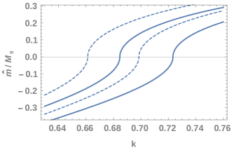
Figure 1: $\hat{m}/M_{s}$ for different values of $\lambda_{0}$, from left to right $\lambda_{0}=0.4,0.001$, $\tan\beta=6,15$ (dashed,thick) and fixed $\kappa\simeq 0.4-0.6$, $M_{\mathrm{s}}=3\,\text{TeV}$.

For $\lambda_{0}\ll 1$ the singlet decouples and the Higgs sector is effectively the Higgs sector of the MSSM. In this case the Higgs mass reaches its upper tree level bound for large values of $\tan\beta$ and thus allows for $M_{\mathrm{s}}={\cal O}(1{\rm TeV})$. From Figure 1 we see that in the regime $\lambda_{0}\ll 1$ and for $0\lesssim\hat{m}\lesssim 0.2\,M_{s}$, the range of the required $k$ take values in the narrow range

$$0.70\lesssim k\lesssim 0.76\quad\text{(effective MSSM)}\ .$$ (26)

On the other hand, a phenomenologically interesting region in the NMSSM corresponds to low $\tan\beta$ and large $\lambda_{0}$. In this regime the tree level value of the Higgs mass is maximized and can take larger values than in the MSSM case. However, too small values of $\tan\beta$ imply a large cancellation of the two terms that contribute to $\hat{m}$ in (10), due to the fact that $m_{h_{d}}^{2}$ is large at low energies. Hence we only consider moderate values of $\tan\beta\,(\simeq 10)$, for which $\hat{m}^{2}\simeq-m_{h_{u}}^{2}$. Analogously, too large values of $\lambda_{0}$ induce large $\mu_{\text{eff}}$, e.g. for $M_{s}=3\text{TeV}$ the upper bound $\lambda_{0}\lesssim 0.4$ corresponds to $\lambda\lesssim 0.33$ and $\mu_{\text{eff}}\lesssim 500\text{GeV}$. Moreover, the upper bound on $\lambda_{0}$ is lessened for larger $M_{s}$. Notice that these constraints exclude the appealing regime of the NMSSM where the Higgs mass can get a larger tree level contribution. Requiring $0\lesssim\hat{m}\lesssim 0.2\,M_{s}$, $5\lesssim\tan\beta\lesssim 15$ and $0.01\lesssim\lambda_{0}\lesssim 0.4$ the range of $k$ widens

$$0.66\lesssim k\lesssim 0.76\quad\text{(NMSSM)}.$$ (27)

The $b_{h}$ parameter can be adjusted to give the desired values of $\tan\beta$. Using (11) and (27) the values of $b_{h}$ that give $5\lesssim\tan\beta\lesssim 20$ are within the range

$$0\lesssim b_{h}/M_{0}^{2}\lesssim 0.4\,.$$ (28)

Finally, in Figure 2 we show that as promised $\hat{m}\ll M_{\mathrm{s}}$ for different values of $\tan\beta$ and $k$.

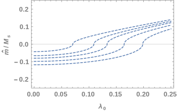
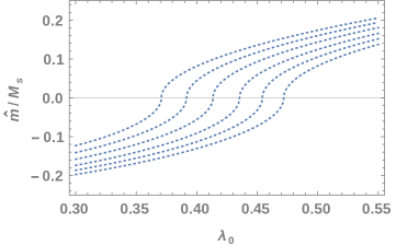
Figure 2: $\hat{m}/M_{\mathrm{s}}$ plotted as a function of $\lambda_{0}$, with $k=0.71$ (upper plot), $k=0.67$ (lower plot), increasing $\tan\beta$ between $6\text{ and }12$ from left to right and with $M_{\mathrm{s}}\simeq 3\text{TeV}$. We see that $\hat{m}$ is $\mathcal{O}(M_{z})$ (region between -0.2 and 0.2) for a broad range of $\tan\beta$ and $\lambda_{0}$.

2.3 Phenomenological implications

In this section we investigate the phenomenological implications of the scenarios studied in section 2.2. In particular, depending on the value of $\lambda_{0}$, we find different predictions that could be tested in the next LHC run.

Using (17) we find that for $M_{\mathrm{s}}\sim 3-6\text{TeV},\,\tan\beta\simeq 10$ the Higgs mass is consistent with the measured value [32, 33] $m_{h}=125.6\text{GeV}$ within an uncertainty of $3\text{GeV}$ and we checked that the mixing of the singlet with the Higgs is negligible in this range of parameters.

The above values of $M_{\mathrm{s}}$ correspond to $M_{0}\sim 1.5-3.5\text{TeV}$. The gluino mass $M_{3}$ obtained from the RGEs and stop masses calculated from (14) are

$${M}_{3}\sim 4-8\text{TeV}\ ,\qquad m_{\tilde{t}_{1,2}}\sim 3-6\text{TeV}\ .$$ (29)

From $M_{3}$ the wino and bino masses are computed via the standard relations [12, 7] $M_{3}:M_{2}:M_{1}\sim 5.5,1.9,1$ giving

$$M_{2}\sim 1400-3000\,\text{GeV},\qquad M_{1}\sim 700-1600\,\text{GeV}\,.$$ (30)

As we already discussed the Higgsino masses scale with $\mu$, which is bounded from below by $100\,\text{GeV}$. Since $\hat{m}$ is of the order of the electroweak scale we need to have $\mu$ in a similar range to obtain the correct Z boson mass. As a consequence the Higgsino masses turn out to be a few hundred GeV.

On the other hand, in the effective MSSM region we find that for very small $\lambda_{0}$ $\mathcal{O}(10^{-4})$ the neutral singlet can become lighter than the Higgs. In this regime, the singlino is the lightest neutralino (see Figure 3). Moreover, a light singlet can yield significant changes in the Higgs decay constants that are consistent with the present LHC bounds. Experimental signatures have been recently studied and provide predictions for the next run [34, 35, 36]. For larger values of $\lambda_{0}$ the singlet and singlino become heavy $\mathcal{O}(\text{TeV})$.

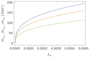
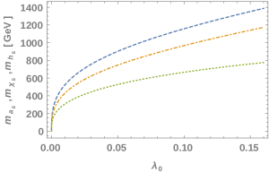
Figure 3: In the left figure we show the masses of the singlet scalar (dashed), singlino (dashed-dotted) and singlet pseudoscalar (dotted) for low values of $\lambda_{0}$ and $M_{s}=3\text{TeV}$. In the right plot the masses of the singlet and singlino are plotted for the same values of $M_{\mathrm{s}}$ and larger values of $\lambda_{0}$. One can see that they rapidly increase with $\lambda_{0}$.

The singlet pseudoscalar turns out to be also very light and its mass strongly depends on the $\lambda_{0}$ coupling (see Figure 3). In the scale invariant version of the NMSSM, the potential exhibits an approximate global $U(1)$ R-symmetry. This symmetry was first discussed in [37] and it is exact at the GUT scale with $A_{\lambda}=A_{\kappa}=0$ as set in (19) and becomes approximate at low energies via the radiative corrections to the A-terms. The symmetry is spontaneously broken when the scalars, $h_{u},h_{d}\text{ and }s$ get a VEV. The corresponding pseudo-Goldstone boson is the singlet pseudoscalar. Here the symmetry is already broken by the $\mu_{h}$ and $b_{h}$ terms terms at the GUT scale, however, provided that these together with $\lambda_{0}$ are small, the mass is slightly corrected from the scale invariant NMSSM case. Moreover, it can modify the Higgs boson decays, the collider signatures of this scenario have been studied and are consistent with present LHC bounds [38, 34, 35, 36, 39].

The spectrum of sleptons and squarks of the first and second generation resembles that of the MSSM in gaugino mediated scenarios [26, 40]. In particular, squarks are heavier than sleptons. The lightest sleptons are the right-handed ones and their masses lie below the bino neutralino within $m_{\tilde{e}_{R}}\simeq 600-1300\,\text{GeV}$.

We cross check the results with a modified version of SPheno [41, 42] created by SARAH [43, 44, 45]. This performs a complete one-loop calculation of all SUSY and Higgs masses and includes the dominant two-loop corrections for the scalar Higgs masses. We show several benchmark points in Table 1, in particular, the spectrum for large $\lambda_{0}$ in P1 and P3, for small $\lambda_{0}$ in P2 and an intermediate value of $\lambda_{0}$ in $P4$.

Parameters	P1	P2	P3	P4
$\lambda_{0}$	0.33	$10^{-4}$	0.1	$10^{-3}$
$M_{0}$ [GeV]	2000	2500	3000	3500
$m_{0}^{2}$ [$\text{GeV}^{2}$]	$7\cdot 10^{6}$	$9.5\cdot 10^{6}$	$1.35\cdot 10^{7}$	$1.75\cdot 10^{7}$
$m_{h_{s}}$ [GeV]	1850	114.5	907.4	178.3
$m_{h}$ [GeV]	123.6	126	125.7	127.9
$m_{H},m_{H^{\pm},m_{A}}$ [GeV]	2824	3434	4067	4660
$m_{a_{s}}$ [GeV]	1040	66.65	561	108.8
$m_{\tilde{\chi}_{s}}$ [GeV]	1659	93.65	814.4	147.8
$m_{\tilde{\chi}_{\mu_{1}}}$ [GeV]	491	695	693	766.2
$m_{\tilde{\chi}_{\mu_{2}}}$ [GeV]	497	700	696	770
$m_{\tilde{\chi}_{\text{bino}}}$ [GeV]	880	1106	1335	1569
$m_{\tilde{\chi}_{\text{wino}}}$ [GeV]	1642	2056	2473	2893
$m_{\tilde{g}}$ [GeV]	4070	5145	6104	7047
$m_{\text{squark}}$ [GeV]	2680-3760	3330-4630	3930-5480	4540-6310
$m_{\text{slepton}}$ [GeV]	667-1300	840-1620	1000-1940	1180-2250

Table 1: Examples of mass spectra computed with SPheno [41, 42] created by SARAH [43, 44, 45]. We used $\tan\beta=15$, $\kappa_{0}=1$ and $M_{s}=3,3.8,4.5,5\text{TeV}$ (from left ro right in the table).

3 Higher dimensional orbifold GUTs

In this section we discuss an orbifold GUT as an example which leads to the previously chosen structure of soft terms in (19) and the relation (22). Let us start by discussing the low energy effective theory.

The starting point is the assumption that the NMSSM is embedded in a higher-dimensional orbifold GUT. In these models a unified gauge group (e.g. $\text{SU}(5)\,\text{or}\,\text{SO}(10)$) in a higher-dimensional theory breaks to the SM gauge group and $N=1$ supersymmetry in four space-time dimensions via the compactification [16, 17, 18, 19, 20]. Thus, $M_{\text{GUT}}\simeq R^{-1}$ where $R$ is the compactification radius. The four-dimensional low energy theory can be such that only the MSSM (or extensions thereof) survive at scales below $R^{-1}$. An important aspect of these higher dimensional theories is that they are non-renormalizable, i.e perturbation theory can only be trusted up to a cutoff scale $\Lambda$.

In order to study phenomenological aspects, it is necessary to specify where the matter content is localized and how supersymmetry breaking occurs. We follow ref. [26] (see also [27, 46]) in that the gauge fields and MSSM Higgses live in the bulk whereas the singlet and the $3^{\text{rd}}$ family of fermions sit at one of the orbifold fix points. The $1^{\text{st}}$ and $2^{\text{nd}}$ fermion generations can be located at the same or a different fixed point.

We consider the situation where a hidden field $\Sigma$ sits at a fixed point which is different from the fixed point of the singlet and the $3^{\text{rd}}$ generation and further assume that $\Sigma$ gets a VEV that triggers supersymmetry breaking [25]. $\Sigma$ is coupled through local universal operators to fields in the bulk which induce soft breaking terms for the latter. However, soft terms for the fields that live on different, separated branes are suppressed at tree level by the size of the extra dimensions and can only develop radiatively. For the localization of fields specified above it implies that soft terms for the singlet and sfermions are negligible while gaugino and Higgs soft scalar masses are sizable and universal. With this setup the theory generates the soft terms in (19) and defines the boundary condition at the GUT scale. Let us now explicitly calculate $m_{0}$ and $M_{0}$ using the expressions given in Appendix A.

The soft terms arise from (non-renormalizable) couplings of the higher-dimensional theory involving $\Sigma$, its $F$-term $F_{\Sigma}$ and the observable fields in the bulk. These couplings rely on the specific mechanism of supersymmetry breaking and they can be computed with the knowledge of the supersymmetric theory at high energies. At low energies the hidden sector decouples, thus the Lagrangian for observable fields reduces to the global supersymmetric piece plus soft terms. The leading order contribution to the soft terms is proportional to the scale

$$m_{\text{soft}}=\frac{F_{\Sigma}}{\Lambda}\ ,$$ (31)

with $F_{\Sigma}$ being the supersymmetry breaking parameter. We follow the approach of [29], i.e. do not specify the dynamics that triggers supersymmetry breaking and parametrize our ignorance through unknown couplings (functions of the hidden field) in the effective Lagrangian. Hence soft terms are given in a model independent way in terms of the Kähler potential $(K)$, the superpotential $(W)$ and the gauge kinetic function $(f)$.

Assuming that the couplings between the hidden field and the observable fields in the bulk are universal we can parametrize $K$, $W$ and $f$ as follows

$$K =Z(\hat{\Sigma},\hat{\bar{\Sigma}})\ (\,|H_{u}|^{2}+|H_{d}|^{2})+(\frac{1}{2}\mu_{K}\,(\hat{\Sigma},\hat{\bar{\Sigma}})H_{u}H_{d}+\text{c.c.})\ ,$$ (32)

$$f =h(\hat{\Sigma})\ ,\quad\text{W}=\mu_{\text{W}}\,(\hat{\Sigma})H_{u}H_{d}\ ,$$

where we defined $\hat{\Sigma}=\frac{\Sigma}{\Lambda}$. Since we do not explicitly know the dynamics of the higher-dimensional theory, the functions $Z,h,\mu_{K},\mu_{\text{W}}$ are unknown.

Via the Giudice-Masiero mechanism [47] the last term in $K$ gives rise to the $\mu_{h}$ and $b_{h}$ parameters. $\mu_{h}$ receives an additional contribution from $\mu_{\text{W}}$ and thus does not have to be of order $m_{\text{soft}}$. Therefore we treat $\mu_{h}$ as a free parameter (i.e. do not address the $\mu$-problem).

After these preliminaries, the calculation of the soft gaugino and soft scalar masses is straightforward by means of (55) and (50) in the appendix. Written in terms of canonically normalized fields, they are given as follows

$$M_{0}=F_{\Sigma}\,\partial_{\Sigma}\log\text{Re}(h)\,,\quad m_{0}^{2}=-|F_{\Sigma}|^{2}\partial_{\Sigma}\bar{\partial}_{\bar{\Sigma}}\log Z\,\ .$$ (33)

From (33) we derive the relation between the soft gaugino and soft higgs masses to be

$$M_{0}=k\,m_{0}\,,\quad k=\frac{\partial_{\Sigma}\log\text{Re}(h)}{(-\partial_{\Sigma}\bar{\partial}_{\bar{\Sigma}}\log Z)^{\frac{1}{2}}}\ .$$ (34)

Furthermore, the leading order contribution of this relation is obtained by expanding $Z$ and $h$ in powers of $\hat{\Sigma},\hat{\bar{\Sigma}}$

$$Z\simeq 1+\rho\,|\hat{\Sigma}|^{2}+\ldots\ ,\quad h\simeq 1+\gamma\hat{\Sigma}+\ldots\ ,$$ (35)

where the numerical coefficients $\rho,\gamma$ are unknown constants. A linear term in Z, $\rho_{1}\,(\hat{\Sigma}+\hat{\bar{\Sigma}})$ can be absorbed in $\rho$ by a field redefinition of the form $H_{u,d}\to(1+\rho_{1})H_{u,d}$ and $\rho\to\rho-\rho_{1}^{2}$. Inserting (35) into (34) yields

$$k=\frac{1}{2}\frac{\gamma}{(-\rho)^{\frac{1}{2}}}\ .$$ (36)

One example where $k$ can be estimated is using Naïve Dimensional Analysis (NDA) [48, 49]. NDA assumes that at the cutoff scale ($\Lambda$) all couplings, and their loop corrections, become order one in units of $\Lambda$, i.e. the theory becomes strongly coupled at energies near $\Lambda$. The corresponding ratio between gaugino and soft scalar masses in this case was computed in [10] and is completely determined in a d-dimensional theory in terms of $\Lambda$ and the volume of the extra dimensions $V_{d-4}$. This relation is explicitly given by

$$M_{0}=k\,m_{0}\,,\quad\mathrm{with}\ k=\left(\frac{l_{d}}{l_{4}\Lambda^{d-4}V_{d-4}}\right)^{\frac{1}{2}},$$ (37)

with $l_{d}$ a numerical factor $l_{d}=2^{d}\pi^{d/2}\Gamma(d/2)$. $\Lambda$ is bounded from above by the Planck scale in d-dimensions, which is defined via

$$M_{\mathrm{P},d}=\left(\frac{M_{\mathrm{P}}^{2}}{V_{d-4}}\right)^{\frac{1}{d-2}}.$$ (38)

We calculate $k$ replacing $V=(2\pi R_{l})^{d}$ with $R_{l}^{-1}\simeq M_{\text{GUT}}$ and $1.24M_{\text{GUT}}\lesssim\Lambda\lesssim M_{\mathrm{P},d}$ (the lower bound of $\Lambda$ is determined by the absence of FCNC, see discussion below). For $d=5$ it yields

$$0.3\lesssim k\lesssim 0.8$$ (39)

and thus provides the coefficient in (27) with the expected size. For $d=6$ or larger the out coming $k$ is smaller than the required values. Notice that $k$ decreases with $\Lambda$, in particular, if $\Lambda$ takes the value of the Planck mass in 5 dimensions $k$ is too small to account for the necessary values.

Let us mention that FCNC in these models are absent as long as the cutoff is sufficiently large. More precisely, dangerous terms are generated through loops in the extra dimensions and scale like $\propto e^{-\Lambda L}$ with $L$ the distance between the branes [46], here $L=2\pi R$. A suppression consistent with experimental bounds ($\lesssim 4\cdot 10^{-4}$) implies $\Lambda L\gtrsim 7.8$, see [26]. Thus, we must require a lower bound on $\Lambda$ of $\Lambda\gtrsim 1.24\,R^{-1}$. On the other hand, as stated above $\Lambda$ is bounded from above by $M_{P,d}$ which, for $V=(2\pi R_{l})^{d}$ and $R_{l}^{-1}\simeq M_{\text{GUT}}$ in $d=5$, yields $\mathcal{O}(10^{17})\text{GeV}$ so the window for $\Lambda$ is quite constraint.

Embedding the NMSSM into a spontaneously broken supergravity yields a gravitino mass $m_{\frac{3}{2}}=\frac{F_{\Sigma}}{\sqrt{3}M_{\mathrm{P}}}$. The relation between $\Lambda$ and $M_{\mathrm{P}}$ is model dependent, however, as long as $\Lambda\ll M_{\mathrm{P}}$ the soft terms that correspond to gravity mediated interactions are sub-leading and thus can be neglected. Moreover, the gravitino mass generically appears as the lightest supersymmetric particle (LSP) and is a good dark matter candidate [50]. For a study on gravitino dark matter in gaugino mediation see [51]. One can estimate $m_{\frac{3}{2}}$ by using $\Lambda$ as in the calculation of soft terms for $d=5$ and $m_{\text{soft}}\simeq M_{0}$. This yields

$$m_{\frac{3}{2}}\simeq\mathcal{O}(0.006-0.06)\,M_{0}.$$ (40)

Replacing $M_{0}$ as calculated in section 2.3 we find $m_{\frac{3}{2}}\simeq 10-100\,\text{GeV}$ and thus the gravitino can be the LSP.

4 Conclusions

In this paper we investigated a special relation among the soft terms that explains the small hierarchy between the supersymmetry breaking scale and the electroweak scale. More precisely, we looked for a condition of the soft terms for which the parameters that trigger electroweak symmetry breaking are suppressed with respect to the supersymmetry breaking scale. We considered the NMSSM and, as boundary conditions at the GUT scale, vanishing soft terms except of gaugino masses and soft terms for the Higgs sector. This setup can be embedded in e.g. higher-dimensional orbifold GUTs where the singlet together with the quarks and leptons are confined to a four dimensional subspace (brane or orbifold fixed point) while the gauge fields and the Higgses propagate in the bulk. Moreover, assuming that supersymmetry breaking occurs at a spatially separated brane by a hidden field leads to the so called gaugino mediation and yields the soft terms at the GUT scale studied in this paper. From the requirement of naturalness explained above we obtained a specific relation between the soft gauginos and Higgs scalar masses.

In addition, we studied the phenomenology of these scenarios. The low energy spectrum depends on the value of the Yukawa coupling $\lambda$ of the singlet. For $\lambda\lesssim\mathcal{O}(10^{-1})$ the singlet scalar and singlino are heavy $\mathcal{O}(\text{TeV})$ while for lower values $\lambda\lesssim\mathcal{O}(10^{-4})$ the singlet becomes the lightest scalar and the singlino the LSP. The pseudoscalar singlet is $\mathcal{O}(100)\text{GeV}$ below $\lambda\lesssim\mathcal{O}(10^{-1})$ and reaches $\mathcal{O}(\text{TeV})$ for larger values of $\lambda$. The gravitino mass is $\mathcal{O}(10)\text{GeV}$ and can be the LSP depending on the value of $\lambda$. These scenarios can also be interesting for dark matter searches.

Furthermore, we derived the soft terms for effective global supersymmetric theories in a model independent way. This class of theories can be considered as an intermediate step of the UV completion and provide the necessary framework in e.g. for gaugino mediated scenarios. We specifically considered the example of [10] where higher-dimensional GUTs provide the special relation between soft gaugino and soft scalar masses required to explain the little hierarchy. This example relies on naïve dimensional analysis arguments which allows to have explicit expressions for the couplings that determine the soft terms. In particular, these depend on the size of the extra dimensions and the cutoff scale and yield the required values for $d=5$ and a cutoff below the Planck mass.

Appendix A Model independent soft terms in non renormalizable theories with global supersymmetry

The starting point is a supersymmetric $N=1$ theory described by two sectors: the observable sector, which includes (extensions of) the MSSM and a hidden sector that is responsible for supersymmetry breaking. The chiral superfields in the observable sector are denoted by $Q^{I}$ while the chiral fields in the hidden sector are called $\phi^{i}$. Arbitrary non-renormalizable couplings are allowed which come suppressed by a cutoff scale $\Lambda$. The Lagrangian can be completely specified in terms of the Kähler potential $K$, the superpotential $W$ and the gauge kinetic function $f$. $K$ is a real and gauge invariant and can be expanded in powers of the chiral fields $Q^{I},\bar{Q}^{\bar{I}}$ which reads

$$K=\Lambda^{2}\hat{K}(\phi,\bar{\phi})+Z_{I\bar{J}}(\phi,\bar{\phi})Q^{I}\bar{Q}^{\bar{J}}+(\frac{1}{2}H_{IJ}(\phi,\bar{\phi})Q^{I}Q^{J}+c.c.)+\ldots\ .$$ (41)

The superpotential is an holomorphic function of the chiral fields which is expanded as

$$W(\phi,Q)=\hat{W}(\phi)+\frac{1}{2}\tilde{\mu}_{IJ}(\phi)Q^{I}Q^{J}+\frac{1}{3}Y_{IJK}(\phi)Q^{I}Q^{J}Q^{K}+...\ .$$ (42)

The gauge kinetic function can depend on the hidden fields and defines the gauge couplings $g^{-2}_{a}(\phi,\bar{\phi})$ where $a$ runs over different factors of the gauge group, i.e. $G=\prod_{a}G_{a}$. The $g_{a}$ renormalize in field theory with an all order expression given by [52, 53]

$$g^{-2}_{a}(\phi,\bar{\phi},p)=\text{Re}f_{a}(\phi) +\frac{b_{a}}{8\pi^{2}}\log\frac{\Lambda}{p}+\frac{T(G_{a})}{8\pi^{2}}\log g^{-2}_{a}(\phi,\bar{\phi},p)$$ (43)

$$-\sum_{r}\frac{T_{a}(r)}{8\pi^{2}}\log\det Z^{(r)}(\phi,\bar{\phi},p)\ .$$

Here $p<\Lambda$ is the renormalization scale and the numerical coefficients are given by $T_{a}(r)=\text{Tr}_{r}(T_{a}^{2})$, $T(G_{a})=T_{a}\text{(adjoint)}$ and $b_{a}=\sum_{r}n_{r}T_{a}(r)-3T(G_{a})$ where the summation is over representations $r$ of the (observable) gauge group G. The first term corresponds to the tree level gauge couplings while the other are loop corrections.

The effective potential of the hidden fields, responsible for supersymmetry breaking, can be written as

$$V^{\text{hid}}\simeq\Lambda^{2}\hat{K}_{i\bar{j}}F^{i}\bar{F}^{\bar{j}}\ ,$$ (44)

where

$$\bar{F}^{\bar{j}}=\Lambda^{-2}\hat{K}^{\bar{j}i}\partial_{i}\hat{W}.$$ (45)

Supersymmetry is spontaneously broken if $\langle F^{i}\rangle\neq 0$ which defines the scale of SUSY breaking via

$$m_{\text{soft}}=\langle\hat{K}_{i\bar{j}}F^{i}\bar{F}^{\bar{j}}\rangle^{\frac{1}{2}}.$$ (46)

Following [29], we calculate the effective Lagrangian for the observable sector. In order to do so, we replace the hidden fields and their auxiliary partners by their VEVs. Keeping only the renormalizable couplings we obtain

$$V(Q,\bar{Q})= \sum_{a}\frac{g_{a}^{2}}{4}(\bar{Q}^{\bar{I}}Z_{\bar{I}J}T_{a}Q^{J})^{2}+\partial_{I}W^{\text{eff}}Z^{I\bar{J}}\bar{\partial}_{\bar{J}}\bar{W}^{\text{eff}}$$ (47)

$$+m_{I\bar{J}}^{2}Q^{I}\bar{Q}^{\bar{J}}+(\frac{1}{3}A_{IJK}Q^{I}Q^{J}Q^{K}+\frac{1}{2}B_{IJ}Q^{I}Q^{J}+c.c.)\ ,$$

where $W^{\text{eff}}$ denotes an effective superpotential defined as follows

$$W^{\text{eff}}(Q)=\frac{1}{2}\mu_{IJ}Q^{I}Q^{J}+\frac{1}{3}Y_{IJK}Q^{I}Q^{J}Q^{K}\ ,$$ (48)

with

$$\mu_{IJ}=\tilde{\mu}_{IJ}-\bar{F}^{\bar{j}}\bar{\partial}_{\bar{j}}H_{IJ}.$$ (49)

From (47) we see that the first two terms correspond to a supersymmetric scalar potential while the last three terms are soft supersymmetry breaking terms. These soft terms depend on the original parameters of the Kähler function and the superpotential via

$$m_{I\bar{J}}^{2} =-F^{i}\bar{F}^{\bar{j}}R_{i\bar{j}I\bar{J}}\ ,$$ (50)

$$A_{IJK} =\ F^{i}D_{i}Y_{IJK}\ ,$$ (51)

$$B_{IJ} =\ F^{i}D_{i}\mu_{IJ}\ ,$$ (52)

with

$$R_{i\bar{j}I\bar{J}}=\partial_{i}\bar{\partial}_{\bar{j}}Z_{I\bar{J}}-\Gamma^{N}_{iI}Z_{N\bar{L}}\bar{\Gamma}^{L}_{\bar{j}\bar{J}}\,,\quad\Gamma^{N}_{iI}=Z^{N\bar{J}}\partial_{i}Z_{\bar{J}I}\ ,$$ (53)

$$D_{i}Y_{IJK}=\partial_{i}Y_{IJK}-\Gamma^{N}_{i(I}Y_{JK)N}\ ,$$

$$D_{i}\mu_{IJ}=\partial_{i}\mu_{IJ}-\Gamma^{N}_{i(I}\mu_{J)N}\ .$$

From (50) one learns that this framework does not guarantee positive soft scalar masses, their sign is model dependent. Another observation is that, as in supergravity, $m_{I\bar{J}}$ need not be universal, hence the appearance of flavor mixing is also a problem in the global case.

The kinetic term of the gauginos is given by

$$g_{a}^{-2}(\phi,\bar{\phi})\,\bar{\lambda}_{a}\sigma^{\mu}D_{\mu}\lambda_{b}\,.$$ (54)

After canonically normalizing the kinetic term of gauginos the soft gaugino masses read

$$\frac{1}{2}(\,M_{a}\lambda^{a}\lambda^{a}+\ c.c.)\ ,\qquad M_{a}=F^{i}\partial_{i}\log g_{a}^{-2}(\phi,\bar{\phi}).$$ (55)

References

- [1] G. Aad et al., “Observation of a new particle in the search for the Standard Model Higgs boson with the ATLAS detector at the LHC,” Phys.Lett., vol. B716, pp. 1–29, 2012, 1207.7214.
- [2] S. Chatrchyan et al., “Observation of a new boson at a mass of 125 GeV with the CMS experiment at the LHC,” Phys.Lett., vol. B716, pp. 30–61, 2012, 1207.7235.
- [3] S. Chatrchyan et al., “Search for supersymmetry in hadronic final states with missing transverse energy using the variables and b-quark multiplicity in pp collisions at TeV,” Eur.Phys.J., vol. C73, no. 9, p. 2568, 2013, 1303.2985.
- [4] G. Aad et al., “Search for new phenomena in final states with large jet multiplicities and missing transverse momentum at =8 TeV proton-proton collisions using the ATLAS experiment,” JHEP, vol. 1310, p. 130, 2013, 1308.1841.
- [5] J. L. Feng, “Naturalness and the Status of Supersymmetry,” Ann.Rev.Nucl.Part.Sci., vol. 63, pp. 351–382, 2013, 1302.6587.
- [6] N. Craig, “The State of Supersymmetry after Run I of the LHC,” 2013, 1309.0528.
- [7] S. P. Martin, “A Supersymmetry primer,” Adv.Ser.Direct.High Energy Phys., vol. 21, pp. 1–153, 2010, hep-ph/9709356.
- [8] D. Horton and G. Ross, “Naturalness and Focus Points with Non-Universal Gaugino Masses,” Nucl.Phys., vol. B830, pp. 221–247, 2010, 0908.0857.
- [9] J. L. Feng, K. T. Matchev, and T. Moroi, “Focus points and naturalness in supersymmetry,” Phys.Rev., vol. D61, p. 075005, 2000, hep-ph/9909334.
- [10] F. Brummer and W. Buchmuller, “A low Fermi scale from a simple gaugino-scalar mass relation,” JHEP, vol. 1403, p. 075, 2014, 1311.1114.
- [11] P. Batra, A. Delgado, D. E. Kaplan, and T. M. Tait, “The Higgs mass bound in gauge extensions of the minimal supersymmetric standard model,” JHEP, vol. 0402, p. 043, 2004, hep-ph/0309149.
- [12] U. Ellwanger, C. Hugonie, and A. M. Teixeira, “The Next-to-Minimal Supersymmetric Standard Model,” Phys.Rept., vol. 496, pp. 1–77, 2010, 0910.1785.
- [13] H. M. Lee, S. Raby, M. Ratz, G. G. Ross, R. Schieren, et al., “Discrete R symmetries for the MSSM and its singlet extensions,” Nucl.Phys., vol. B850, pp. 1–30, 2011, 1102.3595.
- [14] K. Harigaya, T. T. Yanagida, and N. Yokozaki, “Seminatural SUSY from Nonlinear Sigma Model,” 2015, 1504.02266.
- [15] K. Harigaya, T. T. Yanagida, and N. Yokozaki, “Muon g-2 in Focus Point SUSY,” 2015, 1505.01987.
- [16] Y. Kawamura, “Triplet doublet splitting, proton stability and extra dimension,” Prog.Theor.Phys., vol. 105, pp. 999–1006, 2001, hep-ph/0012125.
- [17] G. Altarelli and F. Feruglio, “SU(5) grand unification in extra dimensions and proton decay,” Phys.Lett., vol. B511, pp. 257–264, 2001, hep-ph/0102301.
- [18] A. Hebecker and J. March-Russell, “A Minimal S**1 / (Z(2) x Z-prime (2)) orbifold GUT,” Nucl.Phys., vol. B613, pp. 3–16, 2001, hep-ph/0106166.
- [19] T. Asaka, W. Buchmuller, and L. Covi, “Gauge unification in six-dimensions,” Phys.Lett., vol. B523, pp. 199–204, 2001, hep-ph/0108021.
- [20] L. J. Hall, Y. Nomura, T. Okui, and D. Tucker-Smith, “SO(10) unified theories in six-dimensions,” Phys.Rev., vol. D65, p. 035008, 2002, hep-ph/0108071.
- [21] T. Kobayashi, S. Raby, and R.-J. Zhang, “Constructing 5-D orbifold grand unified theories from heterotic strings,” Phys.Lett., vol. B593, pp. 262–270, 2004, hep-ph/0403065.
- [22] S. Forste, H. P. Nilles, P. K. Vaudrevange, and A. Wingerter, “Heterotic brane world,” Phys.Rev., vol. D70, p. 106008, 2004, hep-th/0406208.
- [23] T. Kobayashi, S. Raby, and R.-J. Zhang, “Searching for realistic 4d string models with a Pati-Salam symmetry: Orbifold grand unified theories from heterotic string compactification on a Z(6) orbifold,” Nucl.Phys., vol. B704, pp. 3–55, 2005, hep-ph/0409098.
- [24] W. Buchmuller, C. Ludeling, and J. Schmidt, “Local SU(5) Unification from the Heterotic String,” JHEP, vol. 0709, p. 113, 2007, 0707.1651.
- [25] L. Randall and R. Sundrum, “Out of this world supersymmetry breaking,” Nucl.Phys., vol. B557, pp. 79–118, 1999, hep-th/9810155.
- [26] Z. Chacko, M. A. Luty, A. E. Nelson, and E. Ponton, “Gaugino mediated supersymmetry breaking,” JHEP, vol. 0001, p. 003, 2000, hep-ph/9911323.
- [27] Z. Chacko, M. A. Luty, and E. Ponton, “Massive higher dimensional gauge fields as messengers of supersymmetry breaking,” JHEP, vol. 0007, p. 036, 2000, hep-ph/9909248.
- [28] M. Schmaltz and W. Skiba, “The Superpartner spectrum of gaugino mediation,” Phys.Rev., vol. D62, p. 095004, 2000, hep-ph/0004210.
- [29] V. S. Kaplunovsky and J. Louis, “Model independent analysis of soft terms in effective supergravity and in string theory,” Phys.Lett., vol. B306, pp. 269–275, 1993, hep-th/9303040.
- [30] U. Ellwanger, “Radiative corrections to the neutral Higgs spectrum in supersymmetry with a gauge singlet,” Phys.Lett., vol. B303, pp. 271–276, 1993, hep-ph/9302224.
- [31] G. G. Ross and K. Schmidt-Hoberg, “The Fine-Tuning of the Generalised NMSSM,” Nucl.Phys., vol. B862, pp. 710–719, 2012, 1108.1284.
- [32] “Updated measurements of the Higgs boson at 125 GeV in the two photon decay channel,” 2013.
- [33] “Combined coupling measurements of the Higgs-like boson with the ATLAS detector using up to 25 fb-1 of proton-proton collision data,” 2013.
- [34] J. Cao, F. Ding, C. Han, J. M. Yang, and J. Zhu, “A light Higgs scalar in the NMSSM confronted with the latest LHC Higgs data,” JHEP, vol. 1311, p. 018, 2013, 1309.4939.
- [35] D. Curtin, R. Essig, and Y.-M. Zhong, “Uncovering light scalars with exotic Higgs decays to bbmumu,” 2014, 1412.4779.
- [36] D. Curtin, R. Essig, S. Gori, P. Jaiswal, A. Katz, et al., “Exotic decays of the 125 GeV Higgs boson,” Phys.Rev., vol. D90, no. 7, p. 075004, 2014, 1312.4992.
- [37] B. A. Dobrescu and K. T. Matchev, “Light axion within the next-to-minimal supersymmetric standard model,” JHEP, vol. 0009, p. 031, 2000, hep-ph/0008192.
- [38] R. Dermisek and J. F. Gunion, “The NMSSM Close to the R-symmetry Limit and Naturalness in..,” Phys.Rev., vol. D75, p. 075019, 2007, hep-ph/0611142.
- [39] N.-E. Bomark, S. Moretti, S. Munir, and L. Roszkowski, “A light NMSSM pseudoscalar Higgs boson at the LHC redux,” 2014, 1409.8393.
- [40] W. Buchmuller, J. Kersten, and K. Schmidt-Hoberg, “Squarks and sleptons between branes and bulk,” JHEP, vol. 0602, p. 069, 2006, hep-ph/0512152.
- [41] W. Porod, “SPheno, a program for calculating supersymmetric spectra, SUSY particle decays and SUSY particle production at e+ e- colliders,” Comput.Phys.Commun., vol. 153, pp. 275–315, 2003, hep-ph/0301101.
- [42] W. Porod and F. Staub, “SPheno 3.1: Extensions including flavour, CP-phases and models beyond the MSSM,” Comput.Phys.Commun., vol. 183, pp. 2458–2469, 2012, 1104.1573.
- [43] F. Staub, “SARAH,” 2008, 0806.0538.
- [44] F. Staub, “From Superpotential to Model Files for FeynArts and CalcHep/CompHep,” Comput.Phys.Commun., vol. 181, pp. 1077–1086, 2010, 0909.2863.
- [45] F. Staub, “Automatic Calculation of supersymmetric Renormalization Group Equations and Self Energies,” Comput.Phys.Commun., vol. 182, pp. 808–833, 2011, 1002.0840.
- [46] D. E. Kaplan, G. D. Kribs, and M. Schmaltz, “Supersymmetry breaking through transparent extra dimensions,” Phys.Rev., vol. D62, p. 035010, 2000, hep-ph/9911293.
- [47] G. Giudice and A. Masiero, “A Natural Solution to the mu Problem in Supergravity Theories,” Phys.Lett., vol. B206, pp. 480–484, 1988.
- [48] A. G. Cohen, D. B. Kaplan, and A. E. Nelson, “Counting 4 pis in strongly coupled supersymmetry,” Phys.Lett., vol. B412, pp. 301–308, 1997, hep-ph/9706275.
- [49] M. A. Luty, “Naive dimensional analysis and supersymmetry,” Phys.Rev., vol. D57, pp. 1531–1538, 1998, hep-ph/9706235.
- [50] W. Buchmuller, V. Domcke, K. Kamada, and K. Schmitz, “A Minimal Supersymmetric Model of Particle Physics and the Early Universe,” pp. 47–77, 2013, 1309.7788.
- [51] W. Buchmuller, L. Covi, J. Kersten, and K. Schmidt-Hoberg, “Dark Matter from Gaugino Mediation,” JCAP, vol. 0611, p. 007, 2006, hep-ph/0609142.
- [52] M. A. Shifman and A. Vainshtein, “Solution of the Anomaly Puzzle in SUSY Gauge Theories and the Wilson Operator Expansion,” Nucl.Phys., vol. B277, p. 456, 1986.
- [53] M. A. Shifman and A. Vainshtein, “On holomorphic dependence and infrared effects in supersymmetric gauge theories,” Nucl.Phys., vol. B359, pp. 571–580, 1991.