Localized density matrix minimization and linear scaling algorithms

Abstract.

We propose a convex variational approach to compute localized density matrices for both zero temperature and finite temperature cases, by adding an entry-wise $\ell_{1}$ regularization to the free energy of the quantum system. Based on the fact that the density matrix decays exponential away from the diagonal for insulating system or system at finite temperature, the proposed $\ell_{1}$ regularized variational method provides a nice way to approximate the original quantum system. We provide theoretical analysis of the approximation behavior and also design convergence guaranteed numerical algorithms based on Bregman iteration. More importantly, the $\ell_{1}$ regularized system naturally leads to localized density matrices with banded structure, which enables us to develop approximating algorithms to find the localized density matrices with computation cost linearly dependent on the problem size.

1. Introduction

Efficient calculation of the low-lying spectrum of operators plays a central role in many applications. In particular, in the context of electronic structure theory, given a discretized effective Hamiltonian (such as the current iterate in a self-consistent iteration), the goal is to obtain the density matrix corresponds to the number of electrons. For zero temperature, the density matrix is the projection operator onto the low-lying eigenspace; for finite temperature, the density matrix is given by the Fermi-Dirac function acting on the Hamiltonian [ParrYang:89, Martin:04].

In this work, we extend the variational approach for localized density matrix in our previous work [LaiLuOsher:15] to finite temperature, by adding entrywise $\ell_{1}$ penalty to the free energy of the quantum system (which, in the context of density functional theory, corresponds to the linear version of the Mermin functional [Mermin:65]). We also theoretically show that the proposed localized density matrix approximates, via the Frobenius norm, the true density matrix linearly depends on the regularization parameter $1/\eta$. In addition, convergence guaranteed numerical algorithms are also designed to solve the proposed problems based on Bregman iteration.

More importantly, this paper focuses on efficient algorithms to minimize the variational problem for localized density matrix both at zero and finite temperature. In particular, we develop linear scaling algorithms such that the computational cost scales linearly as the dimension of the matrix. The key idea is to exploit the decay of the density matrix away from the diagonal, the $\ell_{1}$ regularized localized density matrices enable us to approximate the original variational problem by restricting to banded matrices.

Linear scaling algorithms have been a focused research direction in electronic structure calculation since 1990s. Closely related to our context is the density matrix minimization (DMM) algorithms, first introduced by Li, Nunes, and Vanderbilt [LiNunesVanderbilt:93] and Daw [Daw:93], and have been further developed since then, see e.g., the reviews [Goedecker:99, BowlerMiyazaki:12]. These algorithms are based on the fact that for insulating system or systems at finite temperature, the density matrix decays exponentially away from the diagonal (see e.g., [Kohn:96, ELu:ARMA, Benzi:13]). Thus, one may require the density matrices to satisfy prescribed sparsity structures, such as banded matrices for 1D problem. As a result, the degree of freedom and the computational cost becomes linear scaling. Another closely related class of methods is the purification method of density matrix (see e.g., [McWeeny:60, PalserManolopoulos:98, Niklasson:02, Mazziotti:03] and a review [Niklasson:11]). Unlike the approach of DMM and that we take in this work, these methods are not variational.

We emphasize a crucial difference between our approach and the previous works: Our variational problem is still convex even after truncation! This is in stark contrast to the previous formulations where the convexity is lost by using purification [McWeeny:60] or other techniques to approximate the inverse of density matrix [Challacombe:99]. This loss of convexity often introduces local minimizers to the variational problem and also issues of convergence. We note that even when the $\ell_{1}$ regularization is dropped from our variational problem, it is still convex and different from the standard DMM algorithms. In fact, it would be of interest to explore this convex formulation, which will be considered in our future work.

The rest of the paper is organized as follows. In the next section, we introduce the variational principles for localized density matrix for both zero and finite temperature cases, with their approximation properties. In Section 3, we introduce the Bregman iteration type algorithms to solve these minimization problems. Linear scaling algorithms are discussed in Section 4. We validate the algorithms through numerical examples in Section 5. Some conclusive remarks are discussed in Section 6.

2. Localized density matrix minimization

In this work, we will consider a family of energy functionals with parameters $\beta$ and $\eta$:

(1) $$\mathcal{E}_{\beta,\eta}=\operatorname{tr}(HP)+\frac{1}{\beta}\operatorname{tr}\Big{\{}P\ln P+(1-P)\ln(1-P)\Big{\}}+\frac{1}{\eta}\VERT P\VERT_{1}$$

where $\VERT\cdot\VERT$ denotes the entrywise $\ell_{1}$ norm of a matrix and $H$ and $P$ are $n\times n$ symmetric matrices, which are respectively the (discrete) Hamiltonian and density matrix in the context of electronic structure calculation. Here $\beta$ is the inverse temperature and $\eta$ is the parameter for the $\ell_{1}$ regularization.

Recall that the starting point of [LaiLuOsher:15] is the convex variational principle for density matrix

(2) $$\min_{P\in\mathbb{R}^{n\times n}}\mathcal{E}_{\infty,\infty}(P)=\min_{P\in\mathbb{R}^{n\times n}}\operatorname{tr}(HP),$$

$$\text{s.t.}\quad\operatorname{tr}P=N,\;P=P^{\mathrm{T}},\;0\preceq P\preceq I,$$

where the notation $A\preceq B$ denotes that $B-A$ is a symmetric positive semi-definite matrix. Note that the constraint $0\preceq P\preceq I$ is the convexification of the idempotency constraint $P=P^{2}$, which gives the same minimizer for non-degenerate problems (see e.g., [LaiLuOsher:15]*Proposition 1). Indeed, denote $\{\lambda_{i},\phi_{i}\}_{i=1}^{n}$ the eigenvalue and eigenvector pairs of $H$ with the assumption $\lambda_{N}<\lambda_{N+1}$, the solution of (2) is given by

(3) $$P_{\infty,\infty}=\sum_{i=1}^{N}\phi_{i}\phi_{i}^{\mathrm{T}},$$

the projection operator on the subspace spanned by the first $N$ eigenvectors.

The variational principle (2) corresponds to the physical zero temperature case (and hence the inverse temperature $\beta=\infty$), for finite temperature, we minimize the free energy

(4) $$\min_{P\in\mathbb{R}^{n\times n}}\mathcal{E}_{\beta,\infty}(P)=\min_{P\in\mathbb{R}^{n\times n}}\operatorname{tr}(HP)+\frac{1}{\beta}\operatorname{tr}\Bigl{\{}P\ln P+(1-P)\ln(1-P)\Bigr{\}}$$

$$\text{s.t.}\quad\operatorname{tr}P=N,\;P=P^{\mathrm{T}},\;0\preceq P\preceq I,$$

where we have used the Fermi-Dirac entropy

(5) $$\varphi(x)=x\ln x+(1-x)\ln(1-x),\qquad x\in[0,1].$$

Note that

(6) $$\varphi^{\prime}(x)=\ln x-\ln(1-x),$$

(7) $$\varphi^{\prime\prime}(x)=x^{-1}+(1-x)^{-1},$$

and hence $\varphi^{\prime\prime}(x)\geq 4$ for $x\in[0,1]$. Therefore, $\operatorname{tr}\varphi(P)$ is strictly convex with respect to $P$ and the minimizer of (4) exists and is uniquely given by

(8) $$P_{\beta,\infty}=\Bigl{[}1+\exp(\beta(H-\mu))\Bigr{]}^{-1}=\sum_{i=1}^{n}\rho_{i}\phi_{i}\phi_{i}^{\mathrm{T}},$$

where $\rho_{i}$ is the occupation number of the $i$-th eigenstate, given by

$$\rho_{i}=\frac{1}{1+\exp(\beta(\lambda_{i}-\mu))}\in[0,1],\qquad i=1,\ldots,n,$$

and $\mu$ is the Lagrange multiplier for the constraint $\operatorname{tr}P=N$, known as the chemical potential. It is determined by

$$\sum_{i=1}^{n}\frac{1}{1+\exp(\beta(\lambda_{i}-\mu))}=N.$$

For a fixed Hamiltonian matrix, $\mu$ is then a function of $\beta$. It is not difficult to see that

(9) $$\lim_{\beta\to\infty}\mu(\beta)=\frac{1}{2}(\lambda_{N}+\lambda_{N+1}),$$

which lies in between the highest occupied and lowest unoccupied eigenvalues.

In [LaiLuOsher:15], the following $\ell_{1}$ regularized version of the variaional principle (2) is proposed as a convexified model for compressed modes introduced in [OzolinsLaiCaflischOsher:13].

(10) $$P_{\infty,\eta}= \arg\min_{P\in\mathbb{R}^{n\times n}}\mathcal{E}_{\infty,\eta}=\min_{P\in\mathbb{R}^{n\times n}}\operatorname{tr}(HP)+\frac{1}{\eta}\VERT P\VERT_{1},$$

$$\text{s.t.}\quad\operatorname{tr}P=N,\;P=P^{\mathrm{T}},\;0\preceq P\preceq I,$$

where $\VERT\cdot\VERT_{1}$ is the entrywise $\ell_{1}$ matrix norm and $\eta$ is a penalty parameter for entrywise sparsity. The variational principle provides $P_{\infty,\eta}$ as a sparse representation of the projection operator onto the low-lying eigenspace. Numerical experiments in [LaiLuOsher:15] demonstrate the localization of $P_{\infty,\eta}$ for the above $\ell_{1}$ regularized model.

For the finite temperature, applying the same $\ell_{1}$ regularization to enhance sparsity, we arrive at

(11) $$\min_{P\in\mathbb{R}^{n\times n}}\mathcal{E}_{\beta,\eta}(P)=\min_{P\in\mathbb{R}^{n\times n}}\operatorname{tr}(HP)+\frac{1}{\beta}\operatorname{tr}\Big{\{}P\ln P+(1-P)\ln(1-P)\Big{\}}+\frac{1}{\eta}\VERT P\VERT_{1}$$

$$\text{s.t.}\quad\operatorname{tr}P=N,\;P=P^{\mathrm{T}},\;0\preceq P\preceq I.$$

Since this variational principle is strictly convex, the minimizer exists and is unique.

We will call the minimizing density matrix obtained by the above variational principles the localized density matrix (LDM). We provide in the remaining of this section some approximation results of LDM as the parameter $\eta\to\infty$.

Theorem 1.

Assume $H$ is non-degenerate that $\lambda_{N}<\lambda_{N+1}$ and denote $P_{\infty,\infty}$ the minimizer of (2). Let $P_{\infty,\eta}$ be a minimizer of (10), we have

1. $\displaystyle 0\leq\mathcal{E}_{\infty,\infty}(P_{\infty,\eta})-\mathcal{E}_{\infty,\infty}(P_{\infty,\infty})\leq\frac{1}{\eta}\VERT P_{\infty,\infty}\VERT_{1}$.

2. $\displaystyle\|P_{\infty,\eta}-P_{\infty,\infty}\|_{F}^{2}\leq\frac{2}{\eta}\frac{\VERT P_{\infty,\infty}\VERT_{1}}{(\lambda_{N+1}-\lambda_{N})}$.

In particularly, $\displaystyle\lim_{\eta\rightarrow\infty}\mathcal{E}_{\infty,\infty}(P_{\infty,\eta})=\mathcal{E}_{\infty,\infty}(P_{\infty,\infty})$, and $\displaystyle\lim_{\eta\rightarrow\infty}\left\lVert P_{\infty,\eta}-P_{\infty,\infty}\right\rVert_{F}=0$.

Remark.

Recall that the minimizer of (10) might not be unique [LaiLuOsher:15], nevertheless the theorem applies to any minimizers.

Proof.

It is clear that $\mathcal{E}_{\infty,\infty}(P_{\infty,\infty})\leq\mathcal{E}_{\infty,\infty}(P_{\infty,\eta})$ as $P_{\infty,\infty}$ minimizes the energy $\mathcal{E}_{\infty,\infty}$. On the other hand,since $P_{\eta}$ is an optimizer of (10), we have,

$$\mathcal{E}_{\infty,\infty}(P_{\infty,\eta})\leq\mathcal{E}_{\infty,\infty}(P_{\infty,\eta})+\frac{1}{\eta}\VERT P_{\infty,\eta}\VERT_{1}\leq\mathcal{E}_{\infty,\infty}(P_{\infty,\infty})+\frac{1}{\eta}\VERT P_{\infty,\infty}\VERT_{1}$$

which yields the statement (a).

To show (b), we denote $\{\lambda_{i},\phi_{i}\}_{i=1}^{n}$ the eigenpairs of $H$ and recall that

$$P_{\infty,\infty}=\sum_{1\leq i\leq N}\phi_{i}\phi_{i}^{\mathrm{T}}.$$

Moreover, as $P_{\infty,\eta}$ is symmetric and hence diagonalizable, we denote $\{\sigma_{i},v_{i}\}_{i=1}^{n}$ its eigenpairs, with $P_{\infty,\eta}v_{i}=\sigma_{i}v_{i}$. Note that $\sum_{i}\sigma_{i}=N$ and $\sigma_{i}\in[0,1]$ since $P_{\infty,\eta}$ satisfies the constraint of (10).

Using the property of trace, we calculate

$$\operatorname{tr}(HP_{\infty,\eta})=\sum_{i=1}^{n}\langle\phi_{i},HP_{\infty,\eta}\phi_{i}\rangle=\sum_{i=1}^{n}\lambda_{i}\langle\phi_{i},P_{\infty,\eta}\phi_{i}\rangle=:\sum_{i=1}^{n}\lambda_{i}s_{i},$$

where the last equality defines the shorthand notation $s_{i}=\langle\phi_{i},P_{\infty,\eta}\phi_{i}\rangle$. Since $0\preceq P_{\infty,\eta}\preceq I$ and $\operatorname{tr}P_{\infty,\eta}=N$, we have

$$0\leq s_{i}\leq 1,\qquad\text{and}\qquad\sum_{i=1}^{n}s_{i}=\sum_{i=1}^{n}\langle\phi_{i},P_{\infty,\eta}\phi_{i}\rangle=\operatorname{tr}P_{\infty,\eta}=N.$$

We now estimate, based on these properties of $\{s_{i}\}$,

$$\frac{1}{\eta}\VERT P_{\infty,\infty}\VERT_{1}\geq\mathcal{E}_{\infty,\infty}(P_{\infty,\eta})-\mathcal{E}_{\infty,\infty}(P_{\infty,\infty})\\ =\sum_{j=1}^{n}\lambda_{j}s_{j}-\sum_{j=1}^{N}\lambda_{j}\geq\sum_{j=1}^{N}\lambda_{j}(s_{j}-1)+\sum_{j=N+1}^{n}\lambda_{j}s_{j}\\ \geq\lambda_{N}\sum_{j=1}^{N}(s_{j}-1)+\lambda_{N+1}\sum_{j=N+1}^{n}s_{j}=(\lambda_{N+1}-\lambda_{N})\sum_{j=1}^{N}(1-s_{j}).$$

This yields

(12) $$N-\sum_{j=1}^{N}s_{j}=\sum_{j=1}^{N}(1-s_{j})\leq\frac{1}{\eta}\frac{\VERT P_{\infty,\infty}\VERT_{1}}{(\lambda_{N+1}-\lambda_{N})}.$$

We complete the proof of (b) by

$$\left\lVert P_{\infty,\eta}-P_{\infty,\infty}\right\rVert^{2}_{F} =\operatorname{tr}\Bigl{(}(P_{\infty,\eta}-P_{\infty,\infty})^{2}\Bigr{)}$$

$$=\operatorname{tr}(P_{\infty,\eta}^{2})-2\operatorname{tr}(P_{\infty,\infty}P_{\infty,\eta})+\operatorname{tr}(P_{\infty,\infty}^{2})$$

$$\leq\operatorname{tr}(P_{\infty,\eta})-2\operatorname{tr}(P_{\infty,\infty}P_{\infty,\eta})+\operatorname{tr}(P_{\infty,\infty})$$

$$=2N-2\sum_{i=1}^{n}\langle\phi_{i},P_{\infty,\infty}P_{\infty,\eta}\phi_{i}\rangle$$

$$=2\Bigl{(}N-\sum_{j=1}^{N}s_{j}\Bigr{)}\leq\frac{2}{\eta}\frac{\VERT P_{\infty,\infty}\VERT_{1}}{(\lambda_{N+1}-\lambda_{N})}.$$

∎

For the finite temperature case, we have the following analogous result.

Theorem 2.

Denote $P_{\beta,\infty}$ and $P_{\beta,\eta}$ the minimizer of (4) and (11) respectively, it holds

(13) $$0\leq\mathcal{E}_{\beta,\infty}(P_{\beta,\eta})-\mathcal{E}_{\beta,\infty}(P_{\beta,\infty})\leq\frac{1}{\eta}\VERT P_{\beta,\infty}\VERT_{1},$$

and also the estimate

(14) $$\operatorname{tr}\Bigl{(}\max\bigl{(}\beta^{-1},\left\lvert H-\mu\right\rvert\bigr{)}(P_{\beta,\eta}-P_{\beta,\infty})^{2}\Bigr{)}\leq\frac{1}{\eta}\VERT P_{\beta,\infty}\VERT_{1}.$$

Remark.

Note that as immediate consequence of (14), we have the estimate in Frobenius norm

(15) $$\left\lVert P_{\beta,\eta}-P_{\beta,\infty}\right\rVert_{F}^{2}\leq\frac{1}{\eta}\VERT P_{\beta,\infty}\VERT_{1}\min\bigl{(}\beta,\max_{i}\,\left\lvert\lambda_{i}-\mu\right\rvert^{-1}\bigr{)}.$$

Taking the limit $\beta\to\infty$, as the chemical potential $\mu\to\frac{1}{2}(\lambda_{N}+\lambda_{N+1})$, we get

$$\lim_{\beta\to\infty}\min_{i}\left\lvert\lambda_{i}-\mu\right\rvert\to\frac{\lambda_{N+1}-\lambda_{N}}{2}.$$

Therefore, we recover the estimate for zero temperature case (assuming $\lambda_{N}<\lambda_{N+1}$).

Proof.

By optimality of $P_{\beta,\eta}$ and $P_{\beta,\infty}$, we have $\mathcal{E}_{\beta,\infty}(P_{\beta,\infty})\leq\mathcal{E}_{\beta,\infty}(P_{\beta,\eta})$ and

(16) $$\frac{1}{\eta}\VERT P_{\beta,\infty}\VERT_{1}\geq\mathcal{E}_{\beta,\infty}(P_{\beta,\eta})-\mathcal{E}_{\beta,\infty}(P_{\beta,\infty})\\ =\operatorname{tr}\bigl{(}(P_{\beta,\eta}-P_{\beta,\infty})H\bigr{)}+\beta^{-1}\operatorname{tr}\bigl{(}\varphi(P_{\beta,\eta})-\varphi(P_{\beta,\infty})\bigr{)}.$$

Hence, we obtain the first conclusion (13) of the theorem.

Recall that $\varphi^{\prime}(x)=\ln x-\ln(1-x)$ and hence by explicit calculation using (8)

$$\varphi^{\prime}(P_{\beta,\infty})=\ln\Bigl{(}P_{\beta,\infty}(I-P_{\beta,\infty})^{-1}\Bigr{)}=-\beta(H-\mu).$$

Therefore

$$\operatorname{tr}\bigl{(}(P_{\beta,\eta}-P_{\beta,\infty})H\bigr{)}=\operatorname{tr}\bigl{(}(P_{\beta,\eta}-P_{\beta,\infty})(H-\mu)\bigr{)}=-\beta^{-1}\operatorname{tr}\bigl{(}\varphi^{\prime}(P_{\beta,\infty})(P_{\beta,\eta}-P_{\beta,\infty})\bigr{)},$$

where we have used that $\operatorname{tr}P_{\beta,\eta}=\operatorname{tr}P_{\beta,\infty}=N$ in the first equality. Substitute into (16), we get

(17) $$\frac{1}{\eta}\VERT P_{\beta,\infty}\VERT_{1}\geq\beta^{-1}\Bigl{[}\operatorname{tr}\bigl{(}\varphi(P_{\beta,\eta})-\varphi(P_{\beta,\infty})\bigr{)}-\operatorname{tr}\bigl{(}\varphi^{\prime}(P_{\beta,\infty})(P_{\beta,\eta}-P_{\beta,\infty})\bigr{)}\Bigr{]}$$

Note that the right hand side is the Bregman divergence of $\varphi$. For $x,y\in[0,1]$, we have

$$\varphi(x)-\varphi(y)-\varphi^{\prime}(y)(x-y)=x(\ln x-\ln y)+(1-x)(\ln(1-x)-\ln(1-y)),$$

which is the Fermi-Dirac relative entropy. Following a similar calculation in [HainzlLewinSeiringer:08]*Theorem 1 (see also an improved version in [FrankHainzlSeiringerSolovej:12]), we minimize $x\in[0,1]$ for fixed $y$ and find

$$x\ln\frac{x}{y}+(1-x)\ln\frac{1-x}{1-y}\geq\frac{\ln\frac{1-y}{y}}{1-2y}(x-y)^{2}.$$

Explicit calculation verifies that for $y\in[0,1]$, we have

$$\frac{\ln\frac{1-y}{y}}{1-2y}\geq\max\Bigl{(}\bigl{\lvert}\ln\frac{1-y}{y}\bigr{\rvert},1\Bigr{)}.$$

Hence, combining with (17) and using Klein’s lemma [Ruelle:99]*Theorem 2.5.2, we arrived at the estimate (14)

$$\frac{1}{\eta}\VERT P_{\beta,\infty}\VERT_{1}\geq\operatorname{tr}\Bigl{(}\max\bigl{(}\beta^{-1},\left\lvert H-\mu\right\rvert\bigr{)}(P_{\beta,\eta}-P_{\beta,\infty})^{2}\Bigr{)}.$$

∎

3. Numerical algorithms for LDMs

3.1. Bregman iteration for LDMs

In [LaiLuOsher:15], a numerical algorithm has been proposed to solve (10) based on Bregman iteration. Bregman iteration was first introduced into information science for solving total variation related problems as an analog of “adding back the noise” in image denoising [Osher:2005MMS]. Split Bregman iteration has been later proposed in [Goldstein:2009split] based on the idea of variable splitting. These algorithms have since received intensive attention due to its efficiency in many $\ell_{1}$ related constrained optimization problems [Yin:2008bregman, yin2013error]. The equivalence of the Bregman iteration with the alternating direction method of multipliers (ADMM), Douglas-Rachford splitting and augmented Lagrangian method can be found in [Yin:2008bregman, Esser:2009CAM, Wu:2010SIAM, combettes2011proximal].

Let’s first recall the algorithm proposed in [LaiLuOsher:15]. By introducing auxiliary variables $Q$ and $R$, the optimization problem (10) is equivalent to

(18) $$\min_{P,Q,R\in\mathbb{R}^{n\times n}}\frac{1}{\eta}\VERT Q\VERT_{1}+\operatorname{tr}(HP)$$

$$\text{s.t.}\ Q=P,\,R=P,\,\operatorname{tr}P=N,\,0\preceq R\preceq I,$$

The method of Bregman iteration suggests to approach (18) by solving:

(19) $$(P^{k},Q^{k},R^{k})=\arg\min_{P,Q,R\in\mathbb{R}^{n\times n}}\frac{1}{\eta}\VERT Q\VERT_{1}+\operatorname{tr}(HP)$$

$$\hskip 80.00012pt+\frac{\lambda}{2}\|P-Q+B^{k-1}\|_{F}^{2}+\frac{r}{2}\|P-R+D^{k-1}\|^{2}_{F}$$

$$\qquad\qquad\text{s.t.}\qquad\operatorname{tr}P=N,\,0\preceq R\preceq I,$$

(20) $$B^{k}=B^{k-1}+P^{k}-Q^{k},$$

(21) $$D^{k}=D^{k-1}+P^{k}-R^{k},$$

where variables $B,D$ are essentially Lagrangian multipliers and parameters $r,\lambda$ control the penalty terms. Solving $P^{k},Q^{k},R^{k}$ in (19) alternatively leads to algorithm 3, proposed in [LaiLuOsher:15].

1 Initialize $Q^{0}=R^{0}=P^{0}\in\mathcal{C}=\{P\in\mathbb{R}^{n\times n}~{}|~{}P=P^{\mathrm{T}},\,\operatorname{tr}P=N,\,0\preceq P\preceq I\},B^{0}=D^{0}=0$

2while “not converge” do

3       $\displaystyle P^{k}=\Gamma^{k}-\frac{\operatorname{tr}(\Gamma^{k})-N}{n},\quad\text{where }\Gamma^{k}=\frac{\lambda}{\lambda+r}(Q^{k-1}-B^{k-1})+\frac{r}{\lambda+r}(R^{k-1}-D^{k-1})-\frac{1}{\lambda+r}H$.

4      $\displaystyle Q^{k}=\operatorname{Shrink}\left(P^{k}+B^{k-1},\frac{1}{\lambda\eta}\right)=\operatorname{sign}(P^{k}+B^{k-1})\max\left\{|P^{k}+B^{k-1}|-\frac{1}{\lambda\eta},0\right\}$.

5      $R^{k}=\displaystyle V\min\{\max\{\Lambda,0\},1\}V^{T},\text{ where }[V,~{}\Lambda]=\operatorname{eig}(P^{k}+D^{k-1})$.

6      $B^{k}=B^{k-1}+P^{k}-Q^{k}$.

7      $D^{k}=D^{k-1}+P^{k}-R^{k}$.

Algorithm 3 (Zero temperature localized density matrix minimization).

Similarly, the LDM for the finite temperature case proposed in (11) can also be solved based on Bregman iteration. By introducing auxiliary variables $Q$ and $R$, the optimization problem (11) is equivalent to

(22) $$\min_{P,Q,R\in\mathbb{R}^{n\times n}}\frac{1}{\eta}\VERT Q\VERT_{1}+\operatorname{tr}(HP)+\frac{1}{\beta}\operatorname{tr}\Big{\{}P\ln P+(1-P)\ln(1-P)\Big{\}}$$

$$\text{s.t.}\ Q=P,\,R=P,\,\operatorname{tr}Q=N,\,0\preceq R\preceq I.$$

Note that we have explored the flexibility of the augmenting approach to impose the trace constraint on $Q$, which is equivalent of imposing the constraint on $P$. The minimization (18) can be iteratively solved by:

(23) $$(P^{k},Q^{k},R^{k})=\arg\min_{P,Q,R\in\mathbb{R}^{n\times n}}\frac{1}{\eta}\VERT Q\VERT_{1}+\operatorname{tr}(HP)+\frac{1}{\beta}\operatorname{tr}\Big{\{}P\ln P+(1-P)\ln(1-P)\Big{\}}$$

$$\hskip 60.00009pt+\frac{\lambda}{2}\|P-Q+B^{k-1}\|_{F}^{2}+\frac{r}{2}\|P-R+D^{k-1}\|^{2}_{F}$$

$$\qquad\text{s.t.}\qquad\operatorname{tr}Q=N,\,0\preceq R\preceq I,$$

$$B^{k}=B^{k-1}+P^{k}-Q^{k},$$

$$D^{k}=D^{k-1}+P^{k}-R^{k},$$

where variables $B,D$ and parameters $r,\lambda$ have the similar roles as in (19). Solving $P^{k},Q^{k},R^{k}$ in (23) alternatively leads to the following three sub-optimization problems.

1. $\displaystyle P^{k}=\arg\min_{P\in\mathbb{R}^{n\times n}}\operatorname{tr}(HP)+\frac{1}{\beta}\operatorname{tr}\Big{\{}P\ln P+(1-P)\ln(1-P)\Big{\}}+\frac{\lambda}{2}\|P-Q^{k-1}+B^{k-1}\|_{F}^{2}\\ +\frac{r}{2}\|P-R^{k-1}+D^{k-1}\|^{2}_{F}$.

2. $\displaystyle Q^{k}=\arg\min_{Q\in\mathbb{R}^{n\times n}}\frac{1}{\eta}\VERT Q\VERT_{1}+\frac{\lambda}{2}\|P^{k}-Q+B^{k-1}\|_{F}^{2},\quad\text{s.t.}\quad\operatorname{tr}Q=N$.

3. $R^{k}=\displaystyle\arg\min_{R\in\mathbb{R}^{n\times n}}\|P^{k}-R+D^{k-1}\|^{2}_{F},\quad\text{s.t.}\quad 0\preceq R\preceq I$.

Note that the sub-minimization problem $3^{\circ}$ of algorithm 5 can be solved explicitly, similarly as before

$$R^{k}=V\min\{\max\{\Lambda,0\},1\}V^{T},\text{ where }[V,~{}\Lambda]=\operatorname{eig}(P^{k}+D^{k-1}).$$

To solve the sub-problem $2^{\circ}$ of algorithm 5, let’s denote by $Q_{o}$ the off-diagonal part of $Q$ and write $Q_{d}$ as the diagonal vector of $Q$. Namely, we have $Q=Q_{o}+\mathrm{diag}(Q_{d})$. We also use similar notations for all other matrices. Then the solution of the sub-problem $2^{\circ}$ can be written as $Q^{k}=Q_{o}^{k}+\mathrm{diag}(Q_{d}^{k})$, where $Q_{o}^{k}$ and $Q_{d}^{k}$ are given by (denoting $M^{k}=P^{k}+B^{k-1}$)

(24) $$Q^{k}_{o} =\operatorname{Shrink}\left(M^{k}_{o},(\lambda\eta)^{-1}\right)=\operatorname{sign}(M^{k}_{o})\max\left\{\left\lvert M^{k}_{o}\right\rvert-(\lambda\eta)^{-1},0\right\},$$

(25) $$Q^{k}_{d} =\arg\min_{Q_{d}\in\mathbb{R}^{n}}\frac{1}{\eta}\left\lVert Q_{d}\right\rVert_{1}+\frac{\lambda}{2}\|Q_{d}-M^{k}_{d}\|^{2},\quad\text{s.t.}\quad\ {\bf 1}^{T}Q_{d}=N.$$

here, ${\bf 1}$ is a $n\times 1$ vector with all elements 1. Note that (25) is a convex optimization problem with size $n$, which can be efficiently solved using the following Bregman iteration.

(26) $$Q^{k,s}_{d} =\operatorname{Shrink}\left(\frac{\lambda}{\lambda+r}M^{k}_{d}+\frac{r}{\lambda+r}(v^{s-1}-b^{s-1}),\frac{1}{(\lambda+r)\eta}\right).$$

$$v^{s} =Q^{k,s}_{d}+b^{s-1}-\frac{1}{n}\left({\bf 1}^{T}(Q^{k,s}_{d}+b^{s-1})-N\right).$$

$$b^{s} =b^{s-1}+Q^{k,s}_{d}-v^{s}.$$

Next, we propose to iteratively solve the sub-minimization $1^{\circ}$ in algorithm 5.

(27) $$P^{k}=\arg\min_{P\in\mathbb{R}^{n\times n}}\operatorname{tr}(HP)+\frac{1}{\beta}\operatorname{tr}\Big{\{}P\ln P+(1-P)\ln(1-P)\Big{\}}+\frac{\lambda}{2}\|P-Q^{k-1}+B^{k-1}\|_{F}^{2}\\ +\frac{r}{2}\|P-R^{k-1}+D^{k-1}\|^{2}_{F}.$$

Note that this is a convex problem, and hence the existence of uniqueness of $P^{k}$ is guaranteed. By the KKT condition, $P^{k}$ satisfies

(28) $$H+\frac{1}{\beta}(\ln P^{k}-\ln(1-P^{k}))+\lambda(P^{k}-Q^{k-1}+B^{k-1})+r(P^{k}-R^{k-1}+D^{k-1})=0.$$

Equivalently, we may write the above equation as

(29) $$P^{k}=\Bigl{[}1+\exp\Bigl{(}\beta\bigl{(}H+\lambda(P^{k}-Q^{k-1}+B^{k-1})+r(P^{k}-R^{k-1}+D^{k-1})\bigr{)}\Bigr{)}\Bigr{]}^{-1}.$$

Thus a natural iterative scheme to solve for $P^{k}$ is given by

(30) $$Z^{l+1}=\frac{1}{1+\exp(\beta Y^{l})};$$

(31) $$Y^{l}=H+\lambda(Z^{l}-Q^{k-1}+B^{k-1})+r(Z^{l}-R^{k-1}+D^{k-1}).$$

The following proposition gives the convergence of the above scheme.

Proposition 4.

Assume $\beta(\lambda+r)<4$. Given any symmetric matrices $Q,R,B,D\in\mathbb{R}^{n\times n}$, the iteration scheme

$$Z^{l+1}=\frac{1}{1+\exp(\beta Y^{l})};$$

$$Y^{l}=H+\lambda(Z^{l}-Q+B)+r(Z^{l}-R+D)$$

converges exponentially as $l\to\infty$:

(32) $$\left\lVert Z^{l}-Z^{\ast}\right\rVert=\bigl{(}\beta(\lambda+r)/4\bigr{)}^{l}\left\lVert Z^{0}-Z^{\ast}\right\rVert,$$

where $Z^{\ast}$ is the unique solution of (27).

Proof.

Denote the Fermi-Dirac function

$$\phi_{\beta}(x)=\frac{1}{1+\exp(\beta x)}.$$

We have then

$$\max_{x}\;\left\lvert\phi_{\beta}^{\prime}(x)\right\rvert=\max_{x}\;\left\lvert\frac{\beta\exp(\beta x)}{\bigl{(}1+\exp(\beta x)\bigr{)}^{2}}\right\rvert\leq\beta/4.$$

Therefore,

$$\left\lVert Z^{l+1}-Z^{\ast}\right\rVert=\left\lVert\phi_{\beta}(Y^{l})-\phi_{\beta}(Y^{\ast})\right\rVert\leq\frac{\beta}{4}\left\lVert Y^{l}-Y^{\ast}\right\rVert=\frac{\beta(\lambda+r)}{4}\left\lVert Z^{l}-Z^{\ast}\right\rVert,$$

where $Y^{\ast}=H+\lambda(Z^{\ast}-Q+B)+r(Z^{\ast}-R+D)$. The proposition then follows by iterating with respect to $l$. ∎

In summary, we arrive at algorithm 5 for (11).

1 Initialize $Q^{0}=R^{0}=P^{0}\in\mathcal{C},B^{0}=D^{0}=0$

2while “not converge” do

3       while “not converge” do

4             $Y^{k,l}=H+\lambda(Z^{k,l-1}-Q^{k-1}+B^{k-1})+r(Z^{k,l-1}-R^{k-1}+D^{k-1})$.

5            $\displaystyle Z^{k,l}=\frac{1}{1+\exp(\beta Y^{k,l})}$ .

6      

7      $P^{k}=Z^{k,l}$.

8      $\displaystyle Q^{k}=Q_{o}^{k}+\mathrm{diag}(Q_{d}^{k})$, where $Q_{o}^{k}$ and $Q_{d}^{k}$ are given by (24) and (25).

9      $R^{k}=V\min\{\max\{\Lambda,0\},1\}V^{T},\text{ where }[V,~{}\Lambda]=\operatorname{eig}(P^{k}+D^{k-1})$.

10      $B^{k}=B^{k-1}+P^{k}-Q^{k}$.

11      $D^{k}=D^{k-1}+P^{k}-R^{k}$.

Algorithm 5 (Finite temperature localized density matrix minimization.).

Remark.

In practice, it is not necessary to require all inner iterations convergence in algorithm 5. In our numerical experiments, we run all the inner iterations in algorithm 5 within a given small number of steps, as $Z^{l}$ converges exponentially by Proposition 4.

Theorem 6 (Convergence of Algorithm 3 and Algorithm 5).

1. The sequence $\big{\{}(P^{k},Q^{k},R^{k})\big{\}}_{k}$ generated by algorithm 3 from any starting point converges to a minimum of the variational problem (10).

2. The sequence $\big{\{}(P^{k},Q^{k},R^{k})\big{\}}_{k}$ generated by algorithm 5 from any starting point converges to a minimum of the variational problem (11).

Proof.

The convergence of algorithm 3 is proved in [LaiLuOsher:15]. The proof in fact also applies verbatim to algorithm 5 as it is written for generic convex energy $E(P)$. ∎

While the minimization problems (10) and (11) are convex and the proposed algorithms converge to the minimizers by theorem 6, it is also clear that the computational efficiency of the algorithms 3 and 5 is limited by the eigen-decomposition in the step of eigenvalue thresholding, and also the inner iteration in the finite temperature case. The computational cost for standard eigen-decompsition algorithm is $\mathcal{O}(n^{3})$, which is rather expensive for large scale calculations. In the next section, inspired by ideas from linear scaling algorithms for electronic structure, we propose approximate algorithms to solve (10) and (11) by replacing eigendecompsition with polynomial functions acting on matrices. The resulting algorithms have computational cost linearly scaled with the matrix size $n$.

4. Approximation by banded matrices and linear scaling algorithms

Based on results indicated in theorems 1 and 2, the proposed LDM serves as a nice approximation of the true density matrix. More importantly, similar to many $\ell_{1}$ regularization methods developed for compressed sensing problems, the minimizing density matrices are expected to have certain sparse structure. More precisely, we denote the set of all banded matrices with band width $w$ as

(33) $$\mathcal{B}_{w}=\left\{P=(p_{ij})\in\mathbb{R}^{n\times n}~{}|P=P^{T},p_{ij}=0,~{}\forall~{}j\notin\mathcal{N}^{w}_{i}\right\},$$

where $\mathcal{N}^{w}_{i}$ denotes as a $w$-neighborhood of $i$. In particular, for the $1D$ examples considered later in this paper, the neighborhood is chosen as

$$\mathcal{N}_{i}^{w}=\{j\in\{1,2,\ldots,n\}\mid\left\lvert i-j\right\rvert\mod n\leq w\},$$

for an given band width $w\in\bigl{\{}0,1,2,\cdots,[\frac{n}{2}]\bigr{\}}$ ($w$ is typically chosen much smaller than $n/2$). For example, consider a banded discretized Hamiltonian $H$ (e.g., a central difference discretization of Hamiltonian $-\frac{1}{2}\Delta+V$), numerical results in [LaiLuOsher:15] suggest that the LDM is banded with a small band width. We remark that, however, theoretical validation of this observation is still open and remains to be investigated in future works.

This motivates the following variational problems to approximate the LDMs proposed in (10) and (11) by simply constraining the problems on the set of banded matrices.

(34) $$\min_{P\in\mathbb{R}^{n\times n}}\mathcal{E}^{w}_{\infty,\eta}(P)=\min_{P\in\mathbb{R}^{n\times n}}\operatorname{tr}(HP)+\frac{1}{\eta}\VERT P\VERT_{1},$$

$$\text{s.t.}\quad\operatorname{tr}P=N,\;P=P^{\mathrm{T}},\;0\preceq P\preceq I,\;P\in\mathcal{B}_{w}.$$

(35) $$\min_{P\in\mathbb{R}^{n\times n}}\mathcal{E}^{w}_{\beta,\eta}(P)=\min_{P\in\mathbb{R}^{n\times n}}\operatorname{tr}(HP)+\frac{1}{\beta}\operatorname{tr}\Big{\{}P\ln P+(1-P)\ln(1-P)\Big{\}}+\frac{1}{\eta}\VERT P\VERT_{1}$$

$$\hskip 71.13188pt\text{s.t.}\quad\operatorname{tr}P=N,\;P=P^{\mathrm{T}},\;0\preceq P\preceq I,\;P\in\mathcal{B}_{w}.$$

Note that the above two optimization problems are still convex. This is in contrast to the usual minimization problems developed in the literature of linear scaling algorithms [McWeeny:60, Challacombe:99].

The advantage of considering banded matrix is that it allows for linear scaling algorithms. Let us consider first the eigenvalue thresholding:

(36) $$R=V\min\{\max\{\Lambda,0\},1\}V^{T},\text{ where }[V,~{}\Lambda]=\operatorname{eig}(M).$$

Observe that the above formula can be written as a matrix function

(37) $$R=h(M),\qquad\text{where }h(x)=\min\{\max\{x,0\},1\}=\min\{1/2(|x|+x),1\}.$$

The standard evaluation of the matrix function $h$ using spectral theory needs diagonalization as in (36). The key idea is to approximate general matrix functions by polynomials, as the polynomials acting on matrix only involves products and sums, which can take advantage of the bandedness of the matrix. This type of algorithms has been explored extensively in the literature of linear scaling algorithms (see [GoedeckerColombo:94] and the review articles [Goedecker:99, Niklasson:11, BowlerMiyazaki:12]).

More specifically in the current context, we will approximate the hard thresholding function $h(x)=\min\{1/2(|x|+x),1\}$ using the Chebyshev polynomial approximation [Trefethen:13]. Recall that the standard Chebyshev polynomials approximation minimizes the $L^{\infty}$ error on the interval $[-1,~{}1]$, hence, we will first rescale the matrix such that its eigenvalue lies in the interval.

For this, we first use the power method to estimate the largest eigenvalue $\lambda_{\max}$ and the smallest eigenvalue $\lambda_{\min}$ of $M$. An affine scaling of $M$ gives $s(M)$, whose eigenvalue is in $[-1,1]$, where

$$s(M)=\frac{2}{\lambda_{\max}-\lambda_{\min}}(M-\lambda_{\min})-1.$$

Note that its inverse is given by

$$s^{-1}(M)=\frac{\lambda_{\max}-\lambda_{\min}}{2}M+\frac{\lambda_{\min}+\lambda_{\max}}{2}.$$

We approximate

$$h(M)=h\circ s^{-1}(s(M))\approx T^{m}_{HT}(s(M)),$$

where $T^{m}_{HT}$ is the Chebyshev polynomial approximation of $h\circ s^{-1}$ on $[-1,1]$. Figure 1(a) illustrates the Chebyshev polynomial approximation of $h$ (i.e., $h\circ s^{-1}$ assuming the scaling function $s$ is identity) by $40$ degree polynomials. Higher degree polynomial is needed if $M$ has a larger spectrum span. In our numerical tests, it seems that fixing the degree be $40$ gives satisfactory result for the test examples.

As acting $T^{m}_{HT}$ on $s(M)$ involves matrix products which will increase the matrix band-width. The resulting matrix is projected (with respect to Frobenius norm) on the space $\mathcal{B}_{w}$ to satisfy the constraint. This projection is explicitly given by the truncation operator $\mathfrak{T}_{w}:\mathbb{R}^{n\times n}\rightarrow\mathcal{B}_{w}$ which sets all matrix entries to $0$ outside the $w$-band.

To sum up, the eigenvalue thresholding can be approximated by algorithm 7.

1 $\widehat{P}~{}=~{}$EigenThresviaChebyPoly(P, m)

Input: $P\in\mathcal{B}_{w},~{}m$

Output: $\widehat{P}\in\mathcal{B}_{w}$

2

3Estimate $\lambda_{\max}$ and $\lambda_{\min}$ of $P$ using the power method.

4Compute $T^{m}_{HT}(x)$ as the Chebyshev polynomial approximation of $h\left(\frac{\lambda_{\max}-\lambda_{\min}}{2}x+\frac{\lambda_{\min}+\lambda_{\max}}{2}\right)$.

5$\displaystyle P_{new}=\frac{2}{\lambda_{\max}-\lambda_{\min}}(P-\lambda_{\min})-1$.

$\widehat{P}=\displaystyle\mathfrak{T}_{w}T^{m}_{HT}(P_{new})$.

Algorithm 7 (A linear scaling algorithm for eigenvalue thresholding.).

For banded matrix with band width $w$, the computational cost of this algorithm is $O(nm^{2}w)$ which scale linearly with respect to the matrix dimension $n$. Therefore, for matrices in $\mathcal{B}_{w}$, this algorithm has much better computational efficiency in particular for matrices of large size.

Replacing the eigenvalue thresholding in algorithm 8 by algorithm 7, we obtain the following algorithm for computing LDM in the zero temperature case.

1

2Initialize $Q^{0}=R^{0}=P^{0}\in\mathcal{C}\bigcap\mathcal{B}_{w},B^{0}=D^{0}=0$, choose $m_{et}$.

3while “not converge” do

4       $\displaystyle P^{k}=\Gamma^{k}-\frac{\operatorname{tr}(\Gamma^{k})-N}{n},\quad\text{where }\Gamma^{k}=\frac{\lambda}{\lambda+r}(Q^{k-1}-B^{k-1})+\frac{r}{\lambda+r}(R^{k-1}-D^{k-1})-\frac{1}{\lambda+r}H$.

5      $\displaystyle Q^{k}=\operatorname{Shrink}\left(P^{k}+B^{k-1},\frac{1}{\lambda\eta}\right)$.

6      $R^{k}=\textrm{\sf EigenThresviaChebyPoly}(P^{k}+D^{k-1},m_{et})$.

7      $B^{k}=B^{k-1}+P^{k}-Q^{k}$.

8      $D^{k}=D^{k-1}+P^{k}-R^{k}$.

Algorithm 8 (A linear scaling algorithm for computing LDM at zero temperature.).

We remark that all the steps in algorithm 8 preserves the bandedness of the matrices: For the approximate eigenvalue thresholding, this is guaranteed by the explicit projection step; it can be easily checked for the other steps. Hence, the iterates of the algorithm $(Q,R,P,B,D)$ will remain in $\mathcal{B}_{w}$ as the initial condition lies in the set. Thus, the whole algorithm is linear scaling.

For the finite temperature case, we need a further approximation for evaluating the Fermi-Dirac matrix function $(1+\exp(\beta Y))^{-1}$, as direct computation also involves matrix diagonalization, which is $\mathcal{O}(n^{3})$. Following the same procedure as in algorithm 7, we can achieve a linear scaling algorithm by a Chebyshev polynomial approximation of the Femi-Dirac function $\phi_{\beta}(x)=(1+\exp(\beta x))^{-1}$.

This leads to an algorithm $\textrm{\sf FermiDiracviaChebyPoly}(Y,m)$ for approximating the Fermi-Dirac operation by simply replacing the hard thresholding function $h(x)$ with the Fermi-Dirac function $\phi_{\beta}(x)$ in algorithm 7. Hence, we omit the details. Figure 1(b) shows the approximation of $\phi_{\beta}(x)$ for $\beta=10$ with a degree $40$ polynomial. Nice agreement is observed. We remark that if the temperature is lower (so that $\beta$ is larger), a higher degree polynomial is needed as the function $\phi_{\beta}(x)$ has larger derivatives. In fact, as $\beta\to\infty$, $\phi_{\beta}$ converges to a Heaviside function with jump at $x=0$. Thus, we arrive at the following algorithm 9 for computing LDM of the finite temperature case with linear scaling computation cost with respect to the matrix size $n$.

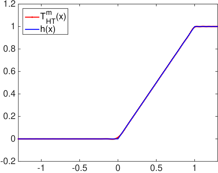
(a)

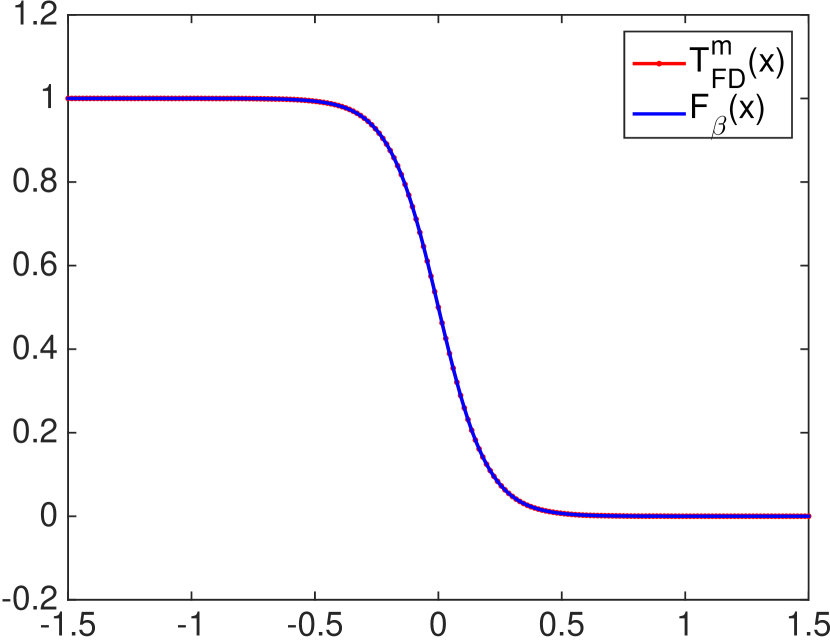
(b)

Figure 1. (a): Chebyshev approximation of $h(x)$ with $m=50$ degree polynomial. (b): Chebyshev approximation of $\phi_{\beta}(x)$ for $\beta=10$ with $m=40$ degree polynomial.

1 Initialize $Q^{0}=R^{0}=P^{0}\in\mathcal{C}\bigcap\mathcal{B}_{w},B^{0}=D^{0}=0$, choose $m_{fd},m_{et}$

2while “not converge” do

3       while “not converge” do

4             $Y^{k,l}=H+\lambda(Z^{k,l-1}-Q^{k-1}+B^{k-1})+r(Z^{k,l-1}-R^{k-1}+D^{k-1})$.

5            $\displaystyle Z^{k,l}=\textrm{\sf FermiDiracviaChebyPoly}(Y^{k,l},m_{fd})$ .

6      

7      $P^{k}=Z^{k,l}$.

8      $\displaystyle Q^{k}=Q_{o}^{k}+\mathrm{diag}(Q_{d}^{k})$, where $Q_{o}^{k}$ and $Q_{d}^{k}$ are given by (24) and (25).

9      $R^{k}=\textrm{\sf EigenThresviaChebyPoly}(P^{k}+D^{k-1},m_{et})$.

10      $b^{k}=B^{k-1}+P^{k}-Q^{k}$.

11      $d^{k}=D^{k-1}+P^{k}-R^{k}$.

Algorithm 9 (A linear scaling algorithm for computing LDM at finite temperature.).

We remark that since polynomial products are applied to approximate the hard thresholding function and the Femi-Dirac operation, approximation errors have been introduced in each iteration of the proposed algorithms 8 and 9. Therefore, the convergence proof used in theorem 6 as we discussed in  [LaiLuOsher:15] can not be directly applied, although our numerical results in Section 5 illustrate satisfactory approximation to model 2 and model 4. Note that similar issues arise in theoretical understanding of convergence of other iterative linear scaling algorithms, for example [GarciaLuXuanE:09].

5. Numerical Experiments

In this section, numerical experiments are presented to demonstrate the proposed models and algorithms for LDM computing for at zero and finite temperatures. We conduct numerical comparisons of our results between LDM computation with and without the linear scaling algorithms, which indicates satisfactory results of the proposed linear scaling algorithms based on approximation by banded matrices. We further illustrate efficiency of the proposed linear scaling algorithms. All numerical experiments are implemented by MATLAB in a PC with a 16G RAM and a 2.7 GHz CPU.

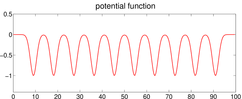
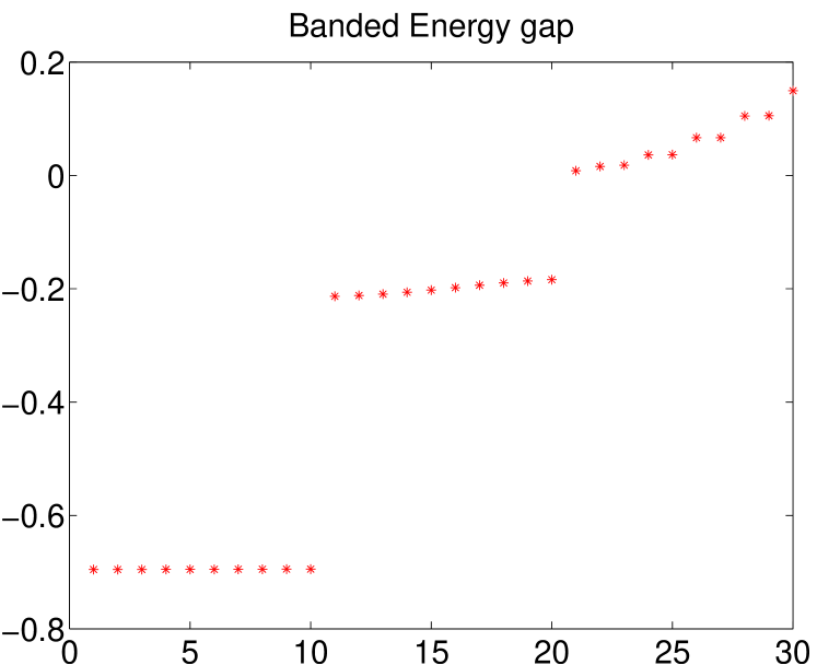
(a)

(b)

Figure 2. (a): The potential function in the modified Kronig-Penney model. (b): The spectrum of the (discretized) Hamiltonian operator.

In our experiments, we consider the proposed models defined on 1D domain $\Omega=[0,~{}100]$ with periodic boundary condition. In this case, the matrix $H$ is a discretization of the Schrödinger operator $\frac{1}{2}\Delta+V$ defined on $\Omega$. Here, $\Delta$ is approximated by a central difference on $[0,~{}100]$ with equally spaced $400$ points. In addition, we consider a modified Kronig–Penney (KP) model [Kronig:1931quantum] for a one-dimensional insulator. The original KP model describes the states of independent electrons in a one-dimensional crystal, where the potential function $V(x)$ consists of a periodic array of rectangular potential wells. We replace the rectangular wells with inverted Gaussians so that the potential is given by

(38) $$V(x)=-V_{0}\sum_{j=1}^{N_{\text{at}}}\exp\left[-\frac{(x-x_{j})^{2}}{\delta^{2}}\right],$$

where $N_{\text{at}}$ gives the number of potential wells. In our numerical experiments, we choose $N_{\text{at}}=10$ and $x_{j}=100j/11$ for $j=1,\ldots,N_{\text{at}}$. The potential is plotted in Figure 2(a). For this given potential, the Hamiltonian operator $H=-\tfrac{1}{2}\Delta+V(x)$ exhibits two low-energy bands separated by finite gaps from the rest of the eigenvalue spectrum (See Figure 2(b)).

The first experiment demonstrates the proposed methods at zero temperature for an insulating case, where we set parameters as $\eta=100,N=10,m_{et}=50$. Figure 3(a) illustrates the true density matrix $\sum_{1\leq i\leq 10}\phi_{i}\phi_{i}^{T}$ obtained by the first $10$ eigenfunctions $\{\phi_{i}\}_{i=1}^{10}$ of $H$. Figure 3(b) plots the density matrix obtained from the proposed model using algorithm 3. As one can observe from Figure 3(b), the LDM provides a quite good approximation to the true density matrix. Note that the LDM with a larger $\eta$ imposes a smaller penalty on the sparsity, and hence the solution has a wider spread and closer to the true density matrix. The approximation behavior is stated in theorem 1. We also refer our previous work [LaiLuOsher:15] for more numerical discussion about this point. Figure 3(c, d) illustrate computing results of LDM using algorithm 8 with band size $w=10,20$ respectively. As we can see from the results, a moderate size of band width can provide satisfactory approximation for the LDM. In addition, we also conduct quantitative comparisons between algorithm 3 and algorithm 8 in table 1, where $P$ and $P_{w}$ are results obtained from algorithm 3 and algorithm 8 respectively. The relative energy error $\frac{|\operatorname{tr}(HP)-\operatorname{tr}(HP_{w})|}{|\operatorname{tr}(HP)|}$ and the comparable relative differences between $\frac{\|P-P_{w}\|_{F}}{\|P\|_{F}}$ and $\frac{\|\mathfrak{T}_{w}(P)-P_{w}\|_{F}}{\|P\|_{F}}$ indicate that results obtained by linear scaling algorithm 8 can provide good estimation of the LDM created from algorithm 3.

(a)

(b)

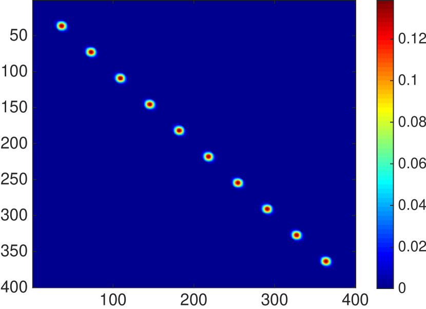
(c)

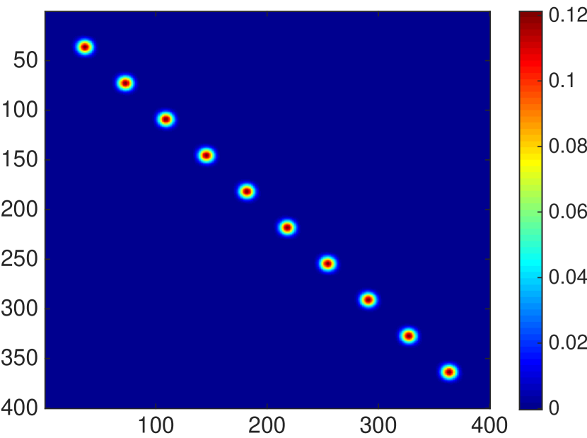
(d)

Figure 3. Result comparisons of the zero temperature case with KP potential ($n=400,N=10$). (a). The true density function obtained by the first N eigenfunctions of $H$. (b). Solution of the localized density matrix with $\eta=100$ using algorithm 3. (c), (d). Solutions of the localized density matrices ($\eta=100$) using algorithm 8 with $w=10,20$ respectively.

For the finite temperature case, it is known that the true density matrix decays exponentially fast along the off-diagonal direction. In the second experiment, we test the algorithms for the finite temperature model with potential free case and modified KP case. We set parameters $\eta=100,\beta=1,m_{et}=40,m_{fd}=20$ for both cases. Figure 4(a) and Figure 5(a) illustrate the corresponding true density matrices described by $\sum_{i}\rho_{i}\phi_{i}\phi_{i}^{T}$ using (8), whose non-zero entries concentrate on a narrow band along the diagonal direction. Figure 4(b) and Figure 5(b) plot the density matrix obtained from the proposed model using algorithm 5. It is clear that the LDM performs reasonably good approximation to the true density matrix. Figure 4(c, d) and Figure 5(c, d) illustrate computing results of LDM using algorithm 9 with band size $w=10,20$ respectively. As we can see from the results, a moderate size of band width can provide satisfactory approximation for the LDM as the true density matrix has exponential decay property. In addition, we also conduct quantitative comparisons between algorithm 5 and algorithm 9 in table 1. The relative energy error $\frac{|\operatorname{tr}(HP)-\operatorname{tr}(HP_{w})|}{|\operatorname{tr}(HP)|}$ and the comparable relative differences between $\frac{\|P-P_{w}\|_{F}}{\|P\|_{F}}$ and $\frac{\|\mathfrak{T}_{w}(P)-P_{w}\|_{F}}{\|P\|_{F}}$ indicate that results obtained by linear scaling algorithm 9 can provide satifactory estimation of the LDM created from algorithm 5.

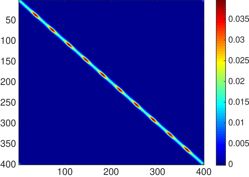
(a)

(b)

(c)

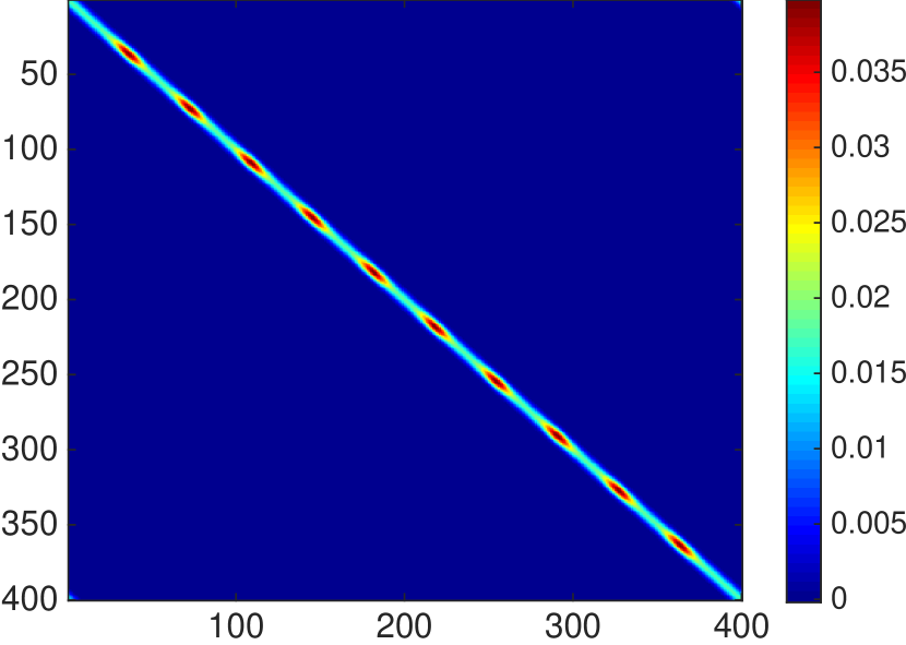
(d)

Figure 4. Result comparisons of the finite temperature case with KP potential ($n=400,N=10,\beta=1$). (a). The true density function obtained by the first N eigenfunctions of $H$. (b). Solution of the localized density matrix with $\eta=100$ using algorithm 5. (c), (d). Solutions of the localized density matrices ($\eta=100$) using algorithm 9 with $w=10,20$ respectively.

(a)

(b)

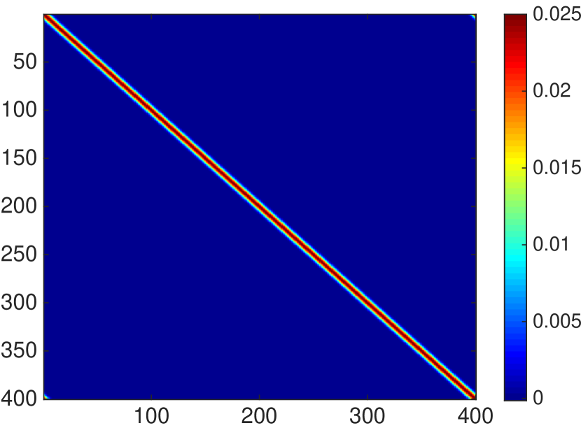
(c)

(d)

Figure 5. Result comparisons of the potential free finite temperature case($n=400,N=10,\beta=1$). (a). The true density function obtained by the first N eigenfunctions of $H$. (b). Solution of the localized density matrix with $\eta=100$ using algorithm 5. (c), (d). Solutions of the localized density matrices ($\eta=100$) using algorithm 9 with $w=10,20$ respectively.

		$\frac{\left\lvert\operatorname{tr}(HP)-\operatorname{tr}(HP_{w})\right\rvert}{\left\lvert\operatorname{tr}(HP)\right\rvert}$	$\frac{|\mathcal{E}_{\beta,\eta}(P)-\mathcal{E}_{\beta,\eta}(P_{w})|}{|\mathcal{E}_{\beta,\eta}(P)|}$	$\frac{\|P-\mathfrak{T}_{w}(P)\|_{F}}{\|P\|_{F}}$	$\frac{\|P-P_{w}\|_{F}}{\|P\|_{F}}$
zero temperature ($\beta=\infty,\eta=100$, modified KP)	$w=10$	$1.00\times 10^{-1}$	$6.36\times 10^{-2}$	$1.46\times 10^{-1}$	$2.32\times 10^{-1}$
	$w=15$	$4.30\times 10^{-2}$	$5.28\times 10^{-2}$	$2.24\times 10^{-2}$	$3.27\times 10^{-2}$
	$w=20$	$4.97\times 10^{-3}$	$1.20\times 10^{-2}$	$1.01\times 10^{-3}$	$1.56\times 10^{-2}$
finite temperature ($\beta=1,\eta=100$, modified KP)	w = 10	$8.31\times 10^{-3}$	$1.44\times 10^{-2}$	$3.86\times 10^{-3}$	$8.46\times 10^{-3}$
	$w=15$	$5.87\times 10^{-4}$	$5.78\times 10^{-4}$	$2.51\times 10^{-4}$	$5.38\times 10^{-4}$
	$w=20$	$9.40\times 10^{-4}$	$4.12\times 10^{-4}$	$1.36\times 10^{-4}$	$3.05\times 10^{-4}$
finite temperature ($\beta=1,\eta=100$, potential free)	w = 10	$2.13\times 10^{-3}$	$2.78\times 10^{-2}$	$4.04\times 10^{-3}$	$5.99\times 10^{-3}$
	$w=15$	$3.03\times 10^{-6}$	$1.03\times 10^{-3}$	$2.66\times 10^{-4}$	$4.81\times 10^{-4}$
	$w=20$	$1.42\times 10^{-5}$	$6.82\times 10^{-4}$	$1.54\times 10^{-4}$	$2.35\times 10^{-4}$

Table 1. Approximation error using banded matrices with $\eta=100$ for all cases.

(a)

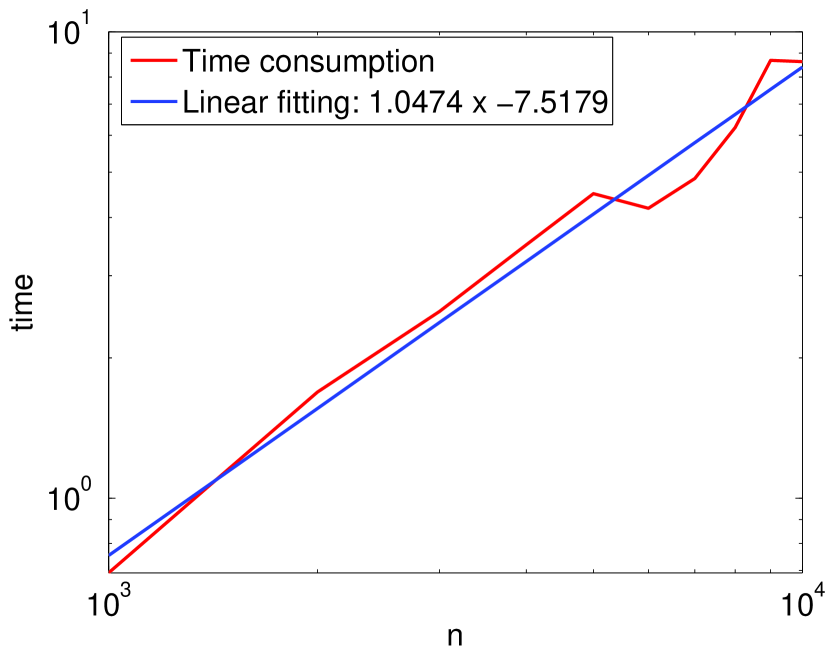
(b)

Figure 6. (a): Time consumption of $\textrm{\sf EigenThresviaChebyPoly}(P,40)$ with different sizes of matrix $P$ and fixed band width $w=10$. (b): Time consumption of $\textrm{\sf FermiDiracviaChebyPoly}(P,40)$ with different sizes of matrix $P$ and fixed band width $w=10$.

In the third experiment, we test the computation cost of the proposed algorithms for approximating the eigenvalue thresholding and the Fermi-Dirac operation. Using different matrix sizes, the EigenThresviaChebyPoly designed by algorithm 7 is applied to approximate the step of hard thresholding eigenvalues used in the algorithm 3 step 5. Similarly, we also test FermiDiracviaChebyPoly for different matrix sizes for the Fermi-Dirac operation. Red curves in Figure 6 (a, b) report log-log curves of the average computation cost for both cases with respect to different matrix sizes, where blue curves illustrate the corresponding linear fitting for the computation cost curve. For banded matrices, It is clear that the computation costs for both approximation algorithms based on Chebyshev polynomials are linear scaling to the matrix sizes.

We next report comparisons for the computation cost of all proposed algorithms, where we set parameters the same as those used in the first and the second experiments. We first conduct comparison between algorithm 3 and algorithm 8 for the zero temperature case with matrix size chosen from $10^{3}$ to $10^{4}$. Figure 7 (a) reports the log-log plots of average time consumption of each iteration for both algorithms. From the slope of the corresponding linear fitting curves, it is clear to see that the original proposed algorithm 3 has computation cost cubically dependent on the matrix size, while the algorithm 8 based on the banded structure has computation cost linearly dependent on the matrix size. As we can observed from Figure 7 (a), the linear scaling algorithm can significantly reduce the computation time when $n$ is larger than certain moderate size. Similarly, we also conduct comparison between algorithm 5 and algorithm 9 for the finite temperature case, where matrices size has been chosen from $10^{2}$ to $2.5\times 10^{3}$. The slopes of the corresponding linear fitting curves also indicate that the proposed algorithm 9 has linear scaling dependent on the problem size, while the original algorithm 5 is cubically scaling to the problem size. Therefore, we can take the linear scaling advantage of the proposed algorithm 8 and algorithm 9 based on the banded structure for problems with large size.

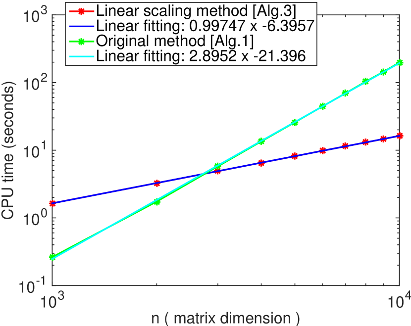
(a)

(b)

Figure 7. (a): Zero temperature case: time consumption of each iteration used in Alg. 3 v.s. Alg. 8. (b): Finite temperature case: time consumption of each iteration used in Alg. 5 v.s. Alg. 9

6. Conclusion and future works

This work extends our previous work [LaiLuOsher:15] for constructing LDMs to the finite temperature case by adding an $\ell_{1}$ regularization to the energy of the original quantum system. As it has been shown that the density matrix decays exponential away from the diagonal for insulating system or system at finite temperature, the LDMs obtained by the proposed convex variational models provide good approximation to the original density matrices. Theoretically, we have conducted analysis to the approximation behavior. In addition, we also design convergence guarantteed numerical algorithms to solve the proposed localized density matrix models based on Bregman iteration. More importantly, by observing that the $\ell_{1}$ regularized system can naturally create a localized density matrix with banded structure, we design approximate algorithms to find the localized density matrices. These numerical algorithms for banded matrices have computation complexity linear scaling to the matrix size $n$.

This paper mainly focuses on proposing variational methods for LDMs, theoretically analyzing its properties and designing numerical algorithms. Thus, we only test some simple examples in the experimental part to illustrate the proposed modes and algorithms. In particular, we have taken a naive finite difference discretization. All codes are implemented in MATLAB for test purpose and are not optimized. In our future work, we will further accelerate the computation from several aspects. First, we can discretize the system using better localized basis to reduce the problem size [FHI-aims, LinLuYingE:DG, Siesta]. Second, we can improve the implementation for better computation performance. In addition, we will explore theoretical analysis for decay properties of the LDM in future works.