Star Formation in Herschel’s Monsters versus Semi-Analytic Models

Abstract

We present a direct comparison between the observed star formation rate functions (SFRF) and the state-of-the-art predictions of semi-analytic models (SAM) of galaxy formation and evolution. We use the PACS Evolutionary Probe Survey (PEP) and Herschel Multi-tiered Extragalactic Survey (HerMES) data-sets in the COSMOS and GOODS-South fields, combined with broad-band photometry from UV to sub-mm, to obtain total (IR$+$UV) instantaneous star formation rates (SFRs) for individual Herschel galaxies up to $z$$\sim$4, subtracted of possible active galactic nucleus (AGN) contamination. The comparison with model predictions shows that SAMs broadly reproduce the observed SFRFs up to $z$$\sim$2, when the observational errors on the SFR are taken into account. However, all the models seem to under-predict the bright-end of the SFRF at $z$${{}_{>}\atop{}^{\sim}}$2. The cause of this underprediction could lie in an improper modelling of several model ingredients, like too strong (AGN or stellar) feedback in the brighter objects or too low fall-back of gas, caused by weak feedback and outflows at earlier epochs.

1 Introduction

The study of how the star formation rate (SFR) in galaxies evolves with redshift provides important constraints to the galaxy formation and evolution theories. In particular, semi-analytic models (SAMs; e.g. White & Frenk 1991; Kauffmann et al. 1993; Springel et al. 2001; Monaco et al. 2007; Guo et al. 2011; Benson 2012; Menci et al. 2012; Henriques et al. 2013), need to be directly compared with observations to obtain insight of the relevant physical processes. The first and most popular SAMs are three, commonly named “Munich” (starting with the models of Kauffmann, White & Guiderdoni 1993), “Durham” (beginning with the models of Cole et al. 1994), and “Santa Cruz” (beginning with the models of Somerville & Primack 1999); more recent SAMs include, i.e., Croton et al. 2006; Bower et al. 2006; Somerville et al. 2008; Fontanot et al. 2009; Guo et al. 2011; Somerville et al. 2012. The main differences between these models lie in the prescriptions adopted for some of the most basic baryonic processes, such as star formation, gas cooling and feedback. One of the processes that must be modelled and compared to data is the evolution of the SFR over the cosmic time. However, the derivation of an accurate SFR from observational data is difficult, due to the many uncertainties involved in its reconstruction. An important source of uncertainty comes from dust extinction. The rest-frame ultraviolet (UV) light emitted by young and massive stars, strictly connected to the instantaneous SFR in galaxies, is strongly absorbed by dust, and re-radiated in the infrared (IR) bands. Dust attenuation, as well as other galaxy physical properties, evolves with cosmic time and shows a peak between $z$$\sim$1 and 2 (e.g. Burgarella et al. 2013). Knowing how dust attenuation evolves in redshift is therefore crucial to study the redshift evolution of the SFR: to this purpose, combining UV information with direct observations in the IR region is probably the best tool to account for the total SFR (e.g., Kennicutt 1998). In fact, IR surveys covering a wide range of redshifts are extremely useful to estimate the global IR luminosity, since they provide a direct measurement of the amount of energy absorbed and re-emitted by dust (e.g., what is missed by UV surveys).

Herschel (Pilbratt et al. 2010), with its 3.5-m mirror, has been the first telescope which allowed us to detect the far-IR population to high redshifts ($z$$\sim$3–4) and to derive its rate of evolution through a detailed LF analysis (Gruppioni et al. 2013; Magnelli et al. 2013) thanks to the extragalactic surveys provided by the Photodetector Array Camera & Spectrometer (PACS; Poglitsch et al. 2010) and Spectral and Photometric Imaging Receiver (SPIRE; Griffin et al. 2010) in the far-IR/sub-mm domain (i.e. PACS Evolutionary Probe, PEP, Lutz et al. 2011; Herschel Multi-tiered Extragalactic Survey, HerMES, Oliver et al. 2012; GOODS-Herschel, Elbaz et al. 2011; Herschel-ATLAS, Eales et al. 2010). PEP and HerMES are the major Herschel Guaranteed Time extragalactic key-projects, designed specifically to determine the cosmic evolution of dusty star formation and of the IR LF, and include the most popular and widely studied extragalactic fields with extensive multi-wavelength coverage available (deep optical, near-IR and Spitzer imaging and spectroscopic and photometric redshifts ; see Berta et al. 2011; Lutz et al. 2011; Oliver et al. 2012 for a detailed description of the fields and observations). The far-IR domain in galaxies, although potentially contaminated by the presence of an AGN, has been probed to be dominated by star formation (i.e. Hatziminaoglou et al. 2010; Delvecchio et al. 2014). Therefore, PEP and HerMES, and all the ancillary data available in the fields, give us the opportunity to disentangle star formation from AGN contribution and to study in detail the evolution of the SFR with cosmic time since the Universe was about a billion years old.
In a recent paper from Pozzi et al. (2015), the observed IR PEP/HerMES LFs have been reproduced by means of a phenomenological model considering two galaxy populations characterised by different evolutions, i.e. a populations of late-type sources and a populations of proto-spheroids. In the model, the IR luminosity functions (linked to the SFR) have been reproduced, as well as the literature K-band luminosity functions (directy linked to the stellar mass), showing that most of the PEP-selected sources observed at $z$$>$2 can be explained as progenitors of local spheroids caught during their formation.
Similar evolutionary rates have been found by Gruppioni et al. (2013), deriving the far- and total IR (i.e. rest-frame 8–1000 $\mu$m) LFs from the Herschel data obtained within the PEP and HerMES projects up to $z$$\sim$4. Since a large fraction of Herschel selected objects have been found to contain an AGN (Berta et al. 2013; Gruppioni et al. 2013; Delvecchio et al. 2014), an accurate quantification of the AGN contribution to the IR luminosity is needed in order to derive reliable SFRs (e.g., not contaminated by AGN activity) from these sources. Delvecchio et al. (2014), through a detailed SED decomposition analysis (see Berta et al. 2013), have disentangled the contribution to the total IR luminosity due to AGN activity and that due to SF for the whole PEP sample. By starting from the work of Delvecchio et al. (2014), but considering the contribution of SF only, in the present paper we focus on the determination of the SFR function (SFRF) and SFR density (SFRD) and compare the results with the predictions of state-of-the-art SAMs of galaxy formation and evolution.

This paper is organised as follows. We discuss the PEP multi-wavelength catalogue in Section 2 and the theoretical predictions and comparison with data in Section 3; finally we present our conclusions in Section 4.

Throughout this paper, we use a Chabrier (2003) initial mass function (IMF) and we assume a $\Lambda$CDM cosmology with $H_{\rm 0}$ = 71 km s^-1 Mpc^-1, $\Omega_{\rm m}$ = 0.27, and $\Omega_{\rm\Lambda}\,=\,0.73$ for data derivations. Note that, although not affecting the results of this paper (see, e.g., Wang et al. 2008), the considered SAMs use slightly different cosmologies.

2 The SFR function of Herschel selected galaxies

2.1 The data-set

We have considered the Herschel PACS (70, 100 and 160 $\mu$m) and SPIRE (250, 350 and 500 $\mu$m) data in the COSMOS and GOODS-S fields from the PEP and HerMES Surveys and all the multi-wavelength data-set associated to the far-IR sources. The reference sample is the PEP blind catalogue selected at 160 $\mu$m to the 3$\sigma$ level, which consists of 4118 and 492 sources respectively in COSMOS (to 10.2 mJy in $\sim$2 deg²) and GOODS-S (to 1.2 mJy in $\sim$196 arcmin². As described in detail by Berta et al. (2011) and Gruppioni et al. (2013), our sources have been associated to the ancillary catalogues by means of a multi-band likelihood ratio technique (e.g., Sutherland & Saunders 1992), starting from the longest available wavelength (160 $\mu$m, PACS) and progressively matching 100 $\mu$m (PACS), 70 $\mu$m (PACS, GOODS-S only) and 24 $\mu$m (Spitzer/MIPS). In the GOODS-S field, we have associated to our PEP sources the 24-$\mu$m catalogue by Magnelli et al. (2009) (extracted with IRAC 3.6-$\mu$m positions as priors), that we have matched with the optical$+$near-IR$+$IRAC MUSIC catalogue of Grazian et al. (2006), revised by Santini et al. (2009), which includes spectroscopic and photometric redshifts. In COSMOS, we have matched our catalogue with the deep 24-$\mu$m sample of Le Floc’h et al. (2009) and with the IRAC-based catalogue of Ilbert et al. (2010), including optical and near-IR photometry and photometric redshifts. In HerMES a prior source extraction was performed using the method presented in Roseboom et al. (2011), based on MIPS-24 $\mu$m positions. The 24-$\mu$m sources used as priors for SPIRE source extraction are the same as those associated with our PEP sources through the likelihood ratio technique. We have therefore associated the HerMES sources with the PEP sources by means of the 24-$\mu$m sources matched to both samples. For most of our PEP sources ($\sim$87 per cent) we found a $>$3$\sigma$ SPIRE counterpart in the HerMES catalogues. Redshifts (either spectroscopic or photometric) are available for all the sources in GOODS-S and for 93% of the COSMOS sample (references and details also in Berta et al. 2011 and Gruppioni et al. 2013).

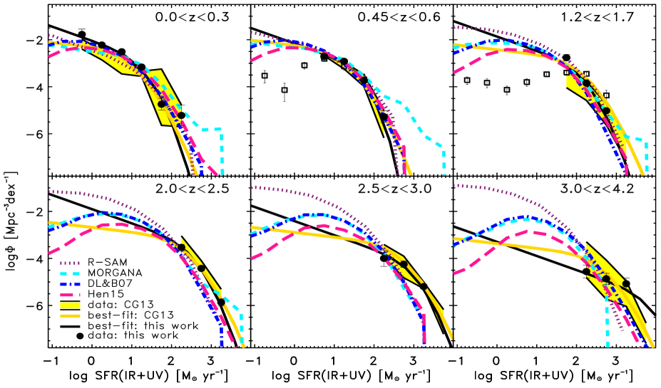
Figure 1: IR$+$UV SFRF estimated through the 1/V_max method in 6 representative redshift bins, by combining the data from the PEP GOODS-S and COSMOS fields using the Avni & Bahcall (1980) technique (black filled circles). The black solid line represents our best fit to our data with a modified Schechter function, while the yellow solid line is the total IR LF (without excluding AGN contribution through SED decomposition) obtained by Gruppioni et al. (2013), converted to a SFRF. The SFRFs of 24-$\mu$m sources with log($M$/$M_{\odot}$)$>$10 in the GOODS-S by Fontanot et al. (2012) are plotted for comparison as black open squares. The SAMS predictions are shown as purple dotted (R-SAM), sea-green short-dashed (MORGANA), blue dot-dashed (De Lucia & Blaizot 2007) and deep-pink long-dashed (Henriques et al. 2015) coloured lines.

2.2 The SFR Function and SFR Density

Gruppioni et al. (2013) derived the far- and total IR (i.e. rest-frame 8–1000 $\mu$m) LFs from the Herschel data obtained within the PEP and HerMES projects up to $z$$\sim$4. To compute the SFRF, we have used the same data and method used by Gruppioni et al. (2013) for deriving the total IR LF, but here we have subtracted - for each source individually - the AGN contribution from each SED, as estimated by Delvecchio et al. (2014), to obtain the IR luminosity due to SF only. In order to disentangle the possible AGN contribution from that related to the host galaxy, Delvecchio et al. (2014) have performed a broad-band SED decomposition of our PEP sources using the MAGPHYS code (da Cunha et al. 2008), which is a public code using physically motivated templates to reproduce the observed galaxy SEDs, as modified by Berta et al. (2013) to include also the AGN component (from Fritz et al. 2006 and Feltre et al. 2012 models). Delvecchio et al. (2014) found significant (at 99 per cent) contribution from AGN in 37 per cent of the PEP sources and used the IR luminosity of the AGN component to derive the AGN bolometric LF and the SMBH growth rate across cosmic time up to $z$$\sim$3. Note that Delvecchio et al. (2014) choose to derive the SMBH accretion function only up to $z$$\sim$3, based on the fact that too few BH accretion data points were available at $z$$>$3 in order to provide an acceptable fit. On the contrary, in this work, we subtract the AGN component from the total IR luminosity of the sources with a significant AGN activity to obtain the contribution due to SF only (L${}_{\rm IR}^{\rm SF}$). In contrast with the work of Delvecchio et al. (2014), we can estimate the SFRF also in the 3$<$$z$$<$4.2 interval, since the SFR data above the completeness limit allowed us to obtain an acceptable fit (though with larger uncertainties than at lower $z$). We have used the same calibration of Santini et al. (2009) and Papovich et al. (2007) to estimate the total instantaneous SFR (then used to derive the SFRF):

$$SFR_{\rm IR+UV}/{\rm M}_{\odot}{\rm yr}^{-1}=1.8\times 10^{-10}\times(2.2\times L_{\rm UV}+L_{\rm IR})$$ (1)

with $L_{\rm UV}$$=$1.5$\times$$L_{\rm 2700\AA}$ computed from the best-fit template SED, and $L_{\rm IR}=$L${}_{\rm IR}^{\rm SF}$. To derive the SFRF, we have used the 1/V_max method (Schmidt et al. 1968), combining the data in the two fields following Avni & Bahcall (1980). According to this method, the SFRF value and its uncertainty in each SFR bin have been computed as:

$$\centering\Phi(SFR,z)=\frac{1}{\Delta SFR}\big{[}\sum_{\rm i}{\frac{1}{w_{\rm i}\times V_{\rm max,i}}}\pm\sqrt{\sum_{\rm i}{\frac{1}{(w_{\rm i}\times V_{\rm max,i})^{2}}}}\big{]}\@add@centering$$ (2)

where $V_{\rm max,i}$ is the comoving volume over which the $i$-${\rm th}$ galaxy could be observed, $\Delta SFR$ is the size of the SFR bin (in logarithmic scale), and $w_{\rm i}$ is the completeness correction factor of the $i$-${\rm th}$ galaxy. These completeness correction factors are a combination of the completeness corrections given by Berta et al. (2011), derived as described in Lutz et al. (2011), to be applied to each source as a function of its flux density, together with a correction for redshift incompleteness. Additional details are given in Gruppioni et al. (2013).

The resulting SFRFs in different redshift intervals are shown in Fig. 1 (black solid circles) and presented in Table 1 (together with their associated 1-$\sigma$ uncertainties). For comparison, the SFRF of sources with log($M$/M_⊙)$>$10 in the GOODS-S derived by Fontanot et al. (2012) have been also plotted, although the two samples have different selections (i.e. the Fontanot et al. 2012 sample is selected at 24 $\mu$m and complete in mass, while ours is flux-limited at 160-$\mu$m), therefore are not directly comparable at the fainter SFRs (affected by the sample cuts). Our best-fit solution with a modified Schechter function (Saunders et al. 1990) has also been reported (black solid line) and compared with the best-fit to the total IR LF of Gruppioni et al. (2013) (yellow solid line), converted to SFRF through the Kennicutt (1998) relation scaled to the Chabrier IMF (although containing also the AGN contribution).

Note that, apart from the two lower redshift bins ($z$$<$0.45), the faint-end of our SFRFs is not constrained by data, therefore we can only derive the value of $\alpha$ at low-$z$, then fix it and keep that value also in the higher redshift bins. This Hobson’s choice implies the assumption that the faint-end slope does not vary with redshift. However, we note that at $z$$<$0.45, where $\alpha$ is constrained by data, the SFRF obtained from the conversion of the total IR LF of Gruppioni et al. (2013) is flatter at low SFRs than the (IR$+$UV) SFRF (e.g. the yellow uncertainty area is lower than the faintest SFR data point). This can be interpreted as due either to a major contribution of the UV to the faint-end (almost negligible at higher SFRs, dominated by the IR) or/and to the fact that some sources might move to fainter luminosity bins when the AGN contribution is removed, thus steepening the SFRF.

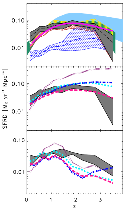
Figure 2: Redshift evolution of the comoving SFRD. The results of integrating the best-fitting curve for our observed IR$+$UV SFRD in each $z$-bin is shown as grey filled area ($\pm$1$\sigma$ uncertainty locus). Top panel: Our IR$+$UV SFRD estimate is compared with other derivations: the yellow line-filled area shows the total IR Luminosity Density resulting from integrating the Gruppioni et al. (2013) best-fitting curve (i.e. converted to SFRD without excluding the AGN contribution); the orange line-filled area shows the uncertainty region of the only-IR SFRD from our data (after AGN removal); the blue line-filled area is the uncorrected for extinction UV SFRD by Cucciati et al. (2012); the dark green filled area is the Burgarella et al. (2013) estimate from Herschel data; the pale blue filled area represents the fit to optical/UV data by Behroozi et al. (2013); the magenta line is the the best-fitting function to IR and UV comoving SFRD by Madau & Dickinson (2014). The honeydew star shows the SFRD value obtained by Marchetti et al. (2015) from the HerMES local wide area sample, by combining the IR and the UV SFRs (but without excluding the AGN contribution). Middle panel: Our IR$+$UV SFRD estimate shown in the previous panel is compared with the SAMs predictions (same colours and line-styles as in the previous figures) integrated over the same range of SFRs (from $log_{10}(SFR)$$=$$-$1.5). Bottom panel: same as in the previous panel, but with our best-fitting function and SAMs integrated only over the SFR range covered by our data.

The latter explanation is also consistent with our finding that in all the redshift bins but the highest one (which is also the most uncertain, due to the high fraction of photometric redshifts), the bright-end of the SFRF (black solid line) is always steeper than that of the total IR LF converted to SFRF (yellow solid line). Since the AGN-dominated sources contribute mainly to the bright-end of the IR LF (see Gruppioni et al. 2013), this difference is due to the subtraction of the AGN component from their SEDs.

The SFRF of 24-$\mu$m selected sources with $M$$>$10¹⁰ M_⊙ by Fontanot et al. (2012) is in good agreement with our determination, in the common redshift and SFR range, with the Fontanot et al. (2012) one being flatter in the lower SFR common bin, likely due to the mass cut in their sample.

Table 1: PEP SFRF and SFRD

	log(${\Phi}$/Mpc-3 dex-1)								$SFRD_{\rm IR+UV}$	$SFRD_{\rm IR}$
									(M⊙ yr-1 Mpc-3)
z	log($SFR_{\rm IR+UV}$/M⊙ yr-1)
	$-$0.5$\div$0.0	0.0$\div$0.5	0.5$\div$1.0	1.0$\div$1.5	1.5$\div$2.0	2.0$\div$2.5	2.5$\div$3.0	3.0$\div$3.5
0.0$-$0.3	$-$1.78$\pm$0.23	$-$2.26$\pm$0.05	$-$2.53$\pm$0.04	$-$3.29$\pm$0.05	$-$4.92$\pm$0.31	$-$5.22$\pm$0.43			0.025$\pm$0.005	0.022$\pm$0.016
0.3$-$0.45		$-$2.52$\pm$0.14	$-$2.36$\pm$0.11	$-$2.85$\pm$0.08	$-$4.29$\pm$0.11	$-$5.22$\pm$0.31			0.035$\pm$0.010	0.028$\pm$0.012
0.45$-$0.6			$-$2.70$\pm$0.09	$-$2.94$\pm$0.06	$-$3.79$\pm$0.05	$-$5.45$\pm$0.31			0.049$\pm$0.014	0.038$\pm$0.013
0.6$-$0.8			$-$2.38$\pm$0.19	$-$2.67$\pm$0.06	$-$3.51$\pm$0.03	$-$4.96$\pm$0.13			0.056$\pm$0.013	0.039$\pm$0.015
0.8$-$1.0				$-$3.01$\pm$0.08	$-$3.26$\pm$0.04	$-$4.40$\pm$0.06	$-$6.17$\pm$0.43		0.064$\pm$0.016	0.050$\pm$0.019
1.0$-$1.2				$-$2.95$\pm$0.11	$-$3.17$\pm$0.08	$-$4.13$\pm$0.04			0.062$\pm$0.014	0.056$\pm$0.026
1.2$-$1.7					$-$2.76$\pm$0.13	$-$3.90$\pm$0.04	$-$5.23$\pm$0.08		0.082$\pm$0.021	0.051$\pm$0.025
1.7$-$2.0						$-$3.96$\pm$0.10	$-$4.61$\pm$0.05	$-$6.56$\pm$0.43	0.071$\pm$0.019	0.062$\pm$0.023
2.0$-$2.5						$-$3.54$\pm$0.13	$-$4.46$\pm$0.06	$-$6.09$\pm$0.19	0.062$\pm$0.021	0.058$\pm$0.015
2.5$-$3.0						$-$4.00$\pm$0.34	$-$4.23$\pm$0.13	$-$5.32$\pm$0.10	0.056$\pm$0.020	0.053$\pm$0.016
3.0$-$4.2						$-$4.67$\pm$0.28	$-$4.94$\pm$0.20	$-$5.34$\pm$0.32	0.028$\pm$0.012	0.016$\pm$0.012

By integrating the best-fitting modified Schechter function to our IR$+$UV (IR) SFRFs down to $log_{10}(SFR)$$=$$-$1.5 in the different redshift bins, from $z$$\sim$0 to $z$$\sim$4, we have derived the comoving IR$+$UV (IR) SFR density (SFRD), as presented in the 10^th (last) column of Table 1 and shown in Fig 2 as a grey-filled (orange line-filled) area. For comparison, other derivations from different bands are shown (i.e. the integration of the best-fitting Schechter function to the total IR LF, containing AGN, converted to SFR as yellow line-filled area; the IR$+$UV SFRD by Burgarella et al. 2013 as dark-green filled area; the fit to optical/UV data by Behroozi et al. 2013 as pale blue filled-area; the UV SFRD - uncorrected for extinction - derivation by Cucciati et al. 2012 as blue line-filled area).

From the comparison between our SFRD and previous derivations, we notice that the IR$+$UV SFRD estimated in this work is higher at low redshift (i.e. $z$$<$0.5), while it agrees within the uncertainties with the other estimates at higher $z$. The IR-only SFRD, given the larger uncertainties, is consistent with the optical SFRD by Behroozi et al. (2013) and with the Gruppioni et al. (2013) IR LD at low-$z$, although the average value is also higher than the latter estimates. Therefore, the low redshift difference is likely due to the UV SFR contribution (that in percentage is higher at low-$z$), but mostly to the AGN contribution subtraction. The (uncorrected for dust extinction) UV SFRD by Cucciati et al. (2012) is significantly lower than our IR or IR$+$UV one over the 0$<$$z$$<$3 range, while at $z$$>$3 it becomes comparable. This is consistent with the peak of dust extinction being around $z$$\sim$1.5-2, with dust attenuation rapidly decreasing at higher redshifts ($>$3-4; e.g., Burgarella et al. 2013). In the top panel of Fig. 2 we also show the redshift evolution of the total SFRDs as obtained (from the same data sample) by Burgarella et al. (2013; dark-green shaded region). The differences (i.e. the Burgarella et al. 2013 estimate is lower than the current one at $z$$<$1 and slightly higher, but still within the uncertainties, at $z$$>$2.5) can be ascribed to the fact that in the previous analysis an average AGN contribution for each population had been subtracted from the total IR luminosity density (then converted to SFRD and summed to the UV SFRD), while in this work an accurate object-by-object subtraction of the IR luminosity contribution due to the AGN has been performed, thanks to the detailed SED-fitting and decomposition of Delvecchio et al. (2014), and a proper SFRF has then been calculated from the obtained IR$+$UV SFRs.

Finally, we note that, while the best-fitting function to the comoving SFRD from IR and UV data by Madau & Dickinson (2014) is in good agreement with our derivation (although slightly lower at $z$$<$0.5 and higher at $z$$>$3), at $z$$>$0.5 the average Behroozi et al. (2013) estimate is always higher (although consistent within the large uncertainty region), maybe due to large extinction corrections.

Finally, in Fig. 2 we show the SFRD value obtained by Marchetti et al. (2015) from the HerMES wide-area sample, by combining the SFR from IR and UV (in analogy with the present work), but without excluding the AGN contribution. The value is in good agreement with the result of Gruppioni et al. (2013) (and the others from the literature) at the same redshift and only marginally consistent with out IR$+$UV SFRD result.

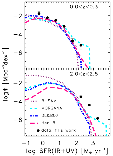
Figure 3: Total (IR$+$UV) SFRF (same as in Fig. 1; black filled circles) in two representative redshift bins compared to SAMs predictions not convolved with an error of 0.3 dex (same colours and line-styles as in Fig. 1).

3 Semi-analytical model predictions

In this section, we compare the observed SFRFs with results obtained with four SAMs of galaxy formation. The SAMs considered in this work are: the MOdel for the Rise of Galaxies aNd Agns (MORGANA, Monaco, Fontanot & Taffoni 2007; sea-green short dashed lines in the figures), R-SAM (Menci et al. 2012, 2014; purple dotted lines) and two versions of the Munich model by De Lucia & Blaizot (2007; dot-dashed blue lines) and Henriques et al. (2015; deep-pink long dashed lines). Note that these SAMs use slightly different cosmologies (see the relative papers for details), although this does not affect the results discussed in this paper (as shown by Wang et al. 2008). Moreover, all the SAMs’ predictions (except the R-SAM’s ones) are mass-limited, with a cut at M$=$10⁹ M${\odot}$, though this selection affects only the low-SFRs, typically lower than those reached by our data. Since these models have not been ”tuned” to reproduce the SFRFs, the results shown in this work can be considered as genuine SAMs predictions.

SAMs treat the physical processes involving baryons (thermal state and infall/outflow of gas, star formation, feedback, accretion onto a black hole, AGN feedback) within the backbone of dark matter (DM) halo merging histories, produced by the gravitational collapse of DM (see Benson 2001 for a review). We refer the reader to the papers cited above for all details on the models.

Together with the observational SFRF, Fig. 1 reports, at the six chosen redshift ranges, the SFRFs predicted by the four SAMs. To take into account the errors in the observational determination of SFRs, model predictions have been convolved with a fiducial error of 0.3 dex (assuming a log-normal error distribution for the SFR with an amplitude of 0.3 dex). As discussed by Fontanot et al. (2009; 2012), this value is roughly equal to the median formal error of SFRs in the GOODS-MUSIC catalogue (Santini et al. 2009) and allows us to determine the gross effect of (random) uncertainties in SFR determinations. We consider this value suitable also for our far-IR-based SFR.

At low redshift ($z$$<$1.7, the three upper panels), all but MORGANA model predictions, are remarkably similar on the bright end. The MORGANA model at $z$${{}_{<}\atop{}^{\sim}}$0.8 shows an excess of very bright sources, that is connected to the specific model of radio-mode AGN feedback, where accretion onto the central black hole takes place from the cold, star forming gas in the bulge, so the suppression of star formation is partial. All models tend to give a power-law tail for the bright-end of the SFRF, that is broadly compatible with the analytical extrapolation of the observed SFRF presented in Section 2. The broadly good agreement between models and data at the bright-end breaks in the very important redshift range from 2 to 3, with the very steep SFRFs produced by all models becoming apparently different from the analytic fit to data in the highest redshift bin. However, the slope of this analytic fit is determined by $z=0-0.3$ data, while at $z\ga 2$, there is clear observational evidence of a steep (or even steepening of the) UV luminosity function (e.g. Cucciati et al. 2012). The consistency at least of one of these models (e.g. MORGANA) with the LF of Lyman-break galaxies has been investigated by Lo Faro et al. (2009). At $z$${{}_{>}\atop{}^{\sim}}$2, the models underpredict the bright-end of the SFRF by a factor of $\sim$0.2$-$0.3 dex. This result depends sensitively on the adopted modelling of observational error. Figure 3 shows the comparison of models and data for two redshift bins at $z$$\sim$0 and $z$$\sim$2, without convolving with 0.3 dex error. While the comparison at $z$$=$0 remains acceptable, the disagreement at $z\sim 2$ worsens dramatically. Only extreme assumptions on the error on SFRs would allow to recover the $z$$\simeq$2 SFRF.

We stress that in the highest redshift bin (3$<$$z$$<$4.2), where the knee of the observed SFRF is not clearly detectable and the shape seems to change significantly, the fraction of photometric redshifts and of the power-law SED AGN (with an uncertain photo-$z$ determination) is higher than at lower $z$’s. For this reason, this $z$-bin is more affected by uncertainties than the other ones and the discrepancy with model predictions here must be taken just as indications (to be furtherly verified).

The inability of SAMs to reproduce the bright-end of the Herschel LF at $z$${{}_{>}\atop{}^{\sim}}$2 had previously been found by Niemi et al. (2012), though based on very preliminary Herschel LF results. It might be connected to the tendency of models to underestimate the main sequence of star-forming galaxies at $z$$\sim$2 (e.g., Dutton et al. 2010). Because SFRs are determined by the complex pattern of gas inflows and outflows, in and out DM halos, and because inflows are determined by outflows taking place at previous times, identifying the cause of this disagreement is not easy. One possibility could be excessive feedback, possibly from AGN either in the radio mode (cooling and thus SFR is over-suppressed in these objects) or in the quasar mode (quasar-triggered outflows limit SFR); however, models with very different implementations of AGN feedback are showing the same problem. Alternatively, an excessive formation of stars in low-mass galaxies (Fontanot et al. 2009; Lo Faro et al. 2009; Weinmann, Neistein & Dekel 2011) could lock too much gas in stars instead of ejecting it from DM halos and making it available for later star formation.

What is interesting to note is that, despite the very different prescriptions for SFR and stellar feedback, all models provide similar predictions (at least up to $z$$\sim$3) in terms of number density of objects with moderate SFRs. Probably this reflects the fact that all the models are calibrated to reproduce the knee of the $z$$=$0 galaxy luminosity/mass function.

At low SFRs ($\la 1$ M_⊙ yr^-1), typically below the completeness limit of Herschel data, models start to separate, with R-SAM and Henriques et al. (2015) giving respectively the highest and lowest SFRFs. These differences may be due to a number of features: different modelling of stellar and AGN feedback, calibration procedure, treatment of merger trees (analytical or based on simulations). The turnover at low SFRs observed in all models but R-SAM is mostly due to incompleteness: models are complete in DM halo mass, that is tightly correlated with stellar mass, while the correlation with SFR is much broader and time-dependent, and this creates a very broad cutoff. While at $z=0$ model SFRFs tend to be lower than the observed ones (as noticed, e.g., by Fontanot et al. 2009), at higher redshifts (but still below $z$$\sim$1.7) they overshoot by a large factor the SFRF of Fontanot et al. (2012), derived for 24-$\mu$m selected sources with $M_{\star}>10^{10}$ M_⊙ in the GOODS-S (but are consistent, up to $z$$\sim$2, with the analytic fit to our SFRF). Part of the difference with Fontanot et al. (2012) is due to the selection in stellar mass done in that paper, which produce a flattening (double-peaked) of the faint-end, although the same paper shows that MORGANA cannot predict the drop in the SFRF at $\sim 1$ M_⊙ yr^-1.

The overprediction of models with respect to the analytic fit to data observed at $log_{10}(SFR){{}_{<}\atop{}^{\sim}}1-2$, becoming more and more important with increasing redshift (although the faint-end slope of the observed SFRSs is fixed at the value found at $z$$\sim$0), if confirmed by deeper data, could be due to the well known excess of low/intermediate mass galaxies predicted by most SAMs with respect to observed mass functions (see, i.e., Somerville & Primack 1999; Cole et al. 2000; Menci et al. 2002; Croton et al. 2006). This aspect is a result of the small-scale power excess typical of the $\Lambda-CDM$ power spectrum (e.g., Moore et al. 1999, Klypin et al. 1999, Menci et al. 2012, Calura et al. 2014). Some authors have suggested that a strong feedback from exploding supernovae can help limiting this excess, and alleviate the discrepancy between data and models at the smallest scales (e.g., Croton et al. 2006; Pontzen & Governato 2012).

The integrals of the SFRFs (SFRD, shown in Figure 2, middle and bottom panels) confirm and better quantify the trends shown in Figure 1. The SFRDs obtained by integrating the SAMs over the same luminosity range as our best-fit SFRFs, are marginally low at $z=0$ for three models out of four (the MORGANA prediction is very close to the observed one, but this is driven by the bright excess visible in Fig. 1). MORGANA and the two Munich models follow the evolution of the observed SFRD up to $z$$\simeq$2, while the R-SAM prediction is significantly steeper, overpredicting the data estimate from $z$$\sim$0.6 up to the higher redshifts. From $z$$=$2 to $z$$=$3 all models but Henriques et al. (2015) overpredict the observed SFRD (at 1-$\sigma$ uncertainty level) by a factor $>$2, with R-SAM diverging by a factor as high as 7–8. Note that if we consider a more conservative uncertainty level for our data (i.e., 3-$\sigma$) the disagreement would be much less or even negligible.

Since the observed SFRD shown in the upper and middle panels of Fig. 2 is obtained by integrating the SFRFs down to SFR values not covered by data, we have also computed the SFRD (from both data and models) by performing the integration just in the SFR range where PEP data are available (as shown in the bottom panel). Here the trend of models underpredicting the observed SFRD at high $z$ is even more evident, with data values starting to be underestimated by SAMs at $z$$\sim$1.5–1.8, but getting closer to model predictions (especially with the Henriques et al. 2015 and R-SAM ones) at $z$$\sim$3.5 (although the better agreement of the 3.2$<$$z$$<$4 SFRD might be due to the compensation of the under-estimate of the bright-end and the over-estimate of the faint-end of the SFRF).

We can conclude that our results at high-$z$ confirm a tension between models and data that possibly points to a problem related to the common assumptions that are at the base of galaxy formation within the $\Lambda$CDM cosmogony. Given the good agreement between models and data at low-$z$, we can interpret these $z$$>$2 tensions as a consequence of model assumptions (like, e.g., the SF law and efficiency, IMF shape) and parameters being calibrated with local observations, and then assumed invariant at higher redshift. It is indeed possible for some of these analytical approximations to have an intrinsic or acquired redshift dependence (through the evolution of the physical properties of model galaxies, see, e.g., Fontanot 2014, where the predicted SFRFs for SAMs with variable IMFs are discussed). Nonetheless, the fact that the largest discrepancies between data and models are seen for the 2$<$$z$$<$3 interval, which represents a peak for both the cosmic SFR and the BH accretion, points to the treatment of SFR in extreme environments as a likely source of the tension. Indeed, the modelling of extreme environments, such those associated with the strongest starburst is still highly uncertain, with many theoretical studies suggesting a different star formation regime for these systems (see, e.g., Somerville, Primack & Faber 2001, Hopkins et al. 2010).
On the other hand, also possible source of uncertainty in the data (affecting mainly the highest redshift interval) might contribute to the tension, increasing the bright-end of the observed SFRF: they can be due to wrong photometric redshifts, bright IR sources at confusion level with flux enhanced by “blending”, mis-identification of lensed galaxies (the latter only to a very minor extent, since the 160-$\mu$m selection should be much less affected by lensed galaxies than sub-mm wavelength ones; e.g. Negrello et al. 2007).

In the future, deeper far-IR observations will be fundamental to explore the faintest end of the SFRF, whereas a study of the bright end at larger redshifts will provide tighter constraints on the feedback processes regulating star formation in the brightest galaxies. A combined study of SFRF and mass function will be also crucial in order to fully understand and tune the single processes considered in SAMs.

4 Conclusions

Starting from the far-IR PEP data considered by Gruppioni et al. (2013), in this paper we investigate the evolution of the SFRF in the redshift range 0.1$<$$z$$<$4 and compare it with theoretical results from various semi-analytical models of galaxy formation (MORGANA, R-SAM, De Lucia & Blaizot 2007 and Henriques et al. 2015). To compute the SFRF, we have subtracted the AGN contribution estimated by Delvecchio et al. (2014) from each SED, to obtain the IR luminosity due to SF only. Then, we have obtained the total instantaneous SFR by combining the IR SF luminosity with the UV derived one, to obtain the total (IR$+$UV) SFR, which we have considered to derive the SFRF.
The conclusions of our work can be summarised as follows.

• We find a generally good agreement between the observed and predicted SFRFs up to $z$$\sim$2 (once the observational errors are taken into account in SAMs), with the exception of MORGANA, showing a high-SFR excess at $z$${{}_{<}\atop{}^{\sim}}$0.8. This result implies that theoretical models, despite the different prescriptions, are able to reproduce the space-density evolution of the IR luminous galaxies from the SFRD peak epoch up to now.

• At $z$${{}_{>}\atop{}^{\sim}}$2, all the models start to under predict the bright-end of the SFRF. This can be due to improper modelling of several ingredients that determine the inflow/outflow patterns of gas in/from DM halos, like AGN feedback, limiting SFR in the largest galaxies, or even inefficient feedback from a previous generation of galaxies.

• Our data are able to constrain the low-SFR end of the (IR$+$UV) SFRF only at low-$z$ ($z$$<$0.45). In this range of redshift, the observed slope is consistent with model predictions, but is steeper than the slope of the total IR LF (containing also AGN contribution) by Gruppioni et al. (2013). However, at intermediate/high-$z$, Herschel data do not sample the low-SFR end of the SFRF, where SAM predictions differ most: our data are not deep enough to allow us to distinguish between the different approaches to SF and stellar feedback considered by the different models. Additional sources of uncertainty affecting the models could be due to the fact that no evolution with redshift is considered for local relations and functions, as SFR laws and IMF. Finally, also data at high redshift could be affected by wrong photometric redshifts and source confusion, contributing to enhance the bright-end of the SFRF, therefore the discrepancy with model predictions.

In this work we have shown that SFRF may help putting stringent constraints on the physical processes modelled in SAMs, especially if extended to low-SFRs, while a study of the bright-end at larger redshifts will provide tighter constraints on the feedback processes regulating star formation in the brightest galaxies. A combined study of SFRF and mass function will be crucial in order to fully understand and tune the single processes modelled in SAMs and to have a global picture of the evolution of SFR and mass growth in galaxies.

References

- Avni & Bahcall (1980) Avni Y. & Bahcall J.N., 1980, ApJ, 235, 694
- Behroozi et al. (2013) Behroozi P.S., Wechsler R.H., Conroy C., 2013, ApJ, 770, 57
- Benson et al. (2001) Benson A.J., Pearce F.R., Frenk C.S., Baugh C.M., Jenkins A., 2001, MNRAS, 320, 261
- Berta et al. (2011) Berta S. et al., 2011, A&A, 532, 49
- Berta et al. (2013) Berta S. et al., 2013, A&A, 551, 100
- Bower et al. (2006) Bower R.G., Benson A.J., Malbon R., Helly J.C., Frenk C.S., Baugh C.M., Cole S. & Lacey C.G., 2006, MNRAS, 370, 645
- Burgarella et al. (2013) Burgarella D. et al., 2013, A&A, 554, 70
- Calura et al. (2014) Calura F., Menci N., Gallazzi A., 2014, MNRAS, 440, 2066
- Chabrier (2003) Chabrier G., 2003, ApJ, 586, L133
- Ciotti & Ostriker (1997) Ciotti L. & Ostriker J.P., 1997, ApJ, 487, L105
- Cole et al. (1994) Cole S., Aragon-Salamanca A., Frenk C.S., Navarro J.F. & Zepf S.E., 1994, MNRAS, 271, 781
- Cole et al. (2000) Cole S., Lacey C.G., Baugh C.M. & Frenk C.S., 2000, MNRAS, 319, 168
- Croton et al. (2006) Croton D.J. et al., 2006, MNRAS, 365, 11
- Cucciati et al. (2012) Cucciati O. et al., 2012, A&A, 539, A31
- da Cunha et al. (2008) da Cunha E., Charlot S. & Elbaz D., 2008, MNRAS, 388, 1595
- Delvecchio et al. (2014) Delvecchio I. et al., 2014, MNRAS, 439, 2736
- De Lucia & Blaizot (2007) De Lucia G. & Blaizot J., 2007, MNRAS, 375, 2
- Dutton et al. (2010) Dutton A.A., van den Bosch F.C. & Dekel A., 2010, MNRAS, 405, 1690
- Eales et al. (2010) Eales S. et al., 2010, PASP, Vol. 122, 891, p. 499
- Elbaz et al. (2011) Elbaz D. et al., 2011, A&A, 533, 119
- Feltre et al. (2012) Feltre A., Hatziminaoglou H., Fritz J. & Franceschini A., 2012, MNRAS, 426, 120
- Fontanot et al. (2009) Fontanot F., De Lucia G., Monaco P., Somerville R.S. & Santini P., 2009, MNRAS, 397, 1776
- Fontanot e Monaco (2010) Fontanot F., Monaco P., 2010, MNRAS, 405, 705
- Fontanot et al. (2012) Fontanot F., Cristiani S., Santini P., Fontana A., Grazian A.& Somerville R.S., 2012, MNRAS, 421, 241
- Fontanot et al. (2013) Fontanot F., Puchwein E., Springel V., Bianchi D., 2013, MNRAS, 436, 2672
- Fontanot (2014) Fontanot F., 2014, MNRAS, 442, 3138
- Fritz et al. (2006) Fritz J., Franceschini, A. & Hatziminaoglou, E., 2006, MNRAS, 366, 767
- Grazian et al. (2006) Grazian A. et al., 2006, A&A, 449, 951
- Griffin et al. (2010) Griffin M. et al., 2010, A&A, 518, L3
- Gruppioni et al. (2013) Gruppioni C. et al., 2013, MNRAS, 423, 23
- Guo et al. (2010) Guo Q., White S., Li C., Boylan-Kolchin M, 2010, MNRAS, 404, 1111
- Guo et al. (2011) Guo Q., White S., Boylan-Kolchin M., De Lucia G., Kauffmann G., Lemson G., Li C., Springel V., Weinmann S., 2011, MNRAS, 413, 101
- Hatziminaoglou et al. (2010) Hatziminaoglou E. et al., 2010, A&A, 518, L33
- Henriques et al. (2013) Henriques B.M.B., White S.D.M., Thomas P.A., Angulo R. E., Guo Q., Lemson G., Springel V., 2013, MNRAS, 431, 3373
- Henriques et al. (2015) Henriques B.M.B., White S.D.M., Thomas P.A., Angulo R. E., Guo Q., Lemson G., Springel V., Overzier R., 2015, MNRAS submitted (arXiv:1410.0365)
- Hopkins & Beacom (2006) Hopkins A.M. & Beacom J.F., 2006, ApJ, 651, 142
- Hopkins et al. (2010) Hopkins P.F., Younger J.D., Hayward C.C., Narayanan D., Hernquist L., 2010, MNRAS, 402, 1693
- Ilbert et al. (2010) Ilbert O. et al., 2010, ApJ, 709, 644
- Kauffmann et al. (1993) Kauffmann G., White S.D.M. & Guiderdoni B., 1993, MNRAS, 264, 201
- Kennicutt (1998) Kennicutt R.C.Jr., 1998, ApJ, 498, 541
- Klypin et al. (1999) Klypin A., Gottlöber S., Kravtsov A.V., Khokhlov A.M., 1999, ApJ, 516, 530
- Le Floc’h et al. (2009) Le Floc’h E. et al., 2009, ApJ, 703, 222
- Lo Faro et al. (2009) Lo Faro B., Monaco P., Vanzella E., Fontanot F., Silva L. & Cristiani S., 2009, MNRAS, 399, 827
- Lutz et al. (2011) Lutz D. et al., 2011, A&A, 532, 90
- Magnelli et al. (2009) Magnelli B., Elbaz D., Chary R.R., Dickinson M., Le Borgne D., Frayer D.T. & Willmer C.N.A., 2009, A&A, 496, 57
- Magnelli et al. (2011) Magnelli B., Elbaz D., Chary R.R., Dickinson M., Le Borgne D., Frayer D.T., & Wilmer C.N.A., 2011, A&A, 528, A35
- Magnelli et al. (2013) Magnelli B. et al., 2013, A&A, 553, A132
- Marchetti et al. (2015) Marchetti L. et al., 2015, MNRAS, submitted
- Menci et al. (2002) Menci N., Cavaliere A., Fontana A., Giallongo E. & Poli F., 2002, ApJ, 575, 18
- Menci et al. (2006) Menci N., Fontana A., Giallongo E., Grazian A., Salimbeni S., 2006, ApJ, 647, 753
- Menci et al. (2008) Menci N., Fiore F., Puccetti S., Cavaliere A., 2008, ApJ, 686, 219
- Menci et al. (2012) Menci N., Fiore F., Lamastra A., 2012, MNRAS, 421, 2384
- Menci et al. (2014) Menci N., Fiore F., Lamastra A., 2014, A&A, 569, 37
- Monaco, Fontanot & Taffoni (2007) Monaco P., Fontanot F., Taffoni G., 2007, MNRAS, 375, 1189
- Moore et al. (1999) Moore B., Ghigna S., Governato F., Lake G., Quinn T., Stadel J., Tozzi P., 1999, ApJ, 524, L19
- Negrello et al. (2007) Negrello M., Perrotta F., Gonz lez-Nuevo Gonz lez J., Silva L., De Zotti G., Granato G.L., Baccigalupi C. & Danese L., 2007, MNRAS, 377, 1557
- Niemi et al. (2012) Niemi S.-M., Somerville R.S., Ferguson H.C., Huang K.-H., Lotz J. & Koekemoer A.M., 2012, MNRAS, 421, 1539
- Oliver et al. (2012) Oliver S. et al., 2012, MNRAS, 424, 1614
- Papovich et al. (2007) apovich C. et al., 2007, ApJ, 668, 45
- Pilbratt et al. (2010) Pilbratt G. et al., 2010, A&A, 518, L1
- Poglitsch et al. (2010) Poglitsch A. et al., 2010, A&A, 518, L2
- Pontzen & Governato (2012) Pontzen A. & Governato F., 2012, MNRAS, 421, 3464
- Pozzi et al. (2015) Pozzi F., Calura F., Gruppioni C., Granato G.L., Cresci G., Silva L., Pozzetti L., Matteucci F., Zamorani G., 2015, ApJ, in press (arXiv:1502.03686)
- Roseboom et al. (2011) Roseboom I.G. et al., 2010, MNRAS, 409, 48
- Santini et al. (2009) Santini P. et al., 2009, A&A, 504, 751
- Saunders et al. (1990) Saunders W. et al., 1990, MNRAS, 242,318
- Schmidt et al. (1968) Schmidt, M. et al., 1968, ApJ, 151, 393
- Somerville & Primack (1999) Somerville R.S. & Primack J.R., 1999, MNRAS, 310, 1087
- Somerville, Primack & Faber (2001) Somerville R.S., Primack J.R. & Faber S.M., 2001, MNRAS, 320, 504
- Somerville et al. (2008) Somerville R.S., Hopkins P.F., Cox T.J., Robertson B.E. & Hernquist L., 2008, MNRAS, 391, 481
- Somerville et al. (2012) Somerville R.S., Gilmore R.C., Primack J.R., Domínguez A., 2012, MNRAS, 2820
- Spergel et al. (2007) Spergel D.N. et al., 2007, ApJS, 170, 377
- Springel et al. (2001) Springel V., White S. D. M., Tormen G., Kauffmann G., 2001, MNRAS, 328, 726
- Springel et al. (2005) Springel V., Di Matteo T., Hernquist L., 2005, MNRAS, 361, 776
- Sutherland & Saunders (1992) Sutherland, W. & Saunders, W., 1992, MNRAS, 259, 413
- Wang & Kauffmann (2008) Wang L. & Kauffmann G., 2008, MNRAS, 391, 785
- Wang et al. (2008) Wang J., De Lucia G., Kitzbichler M.G., White S.D.M., 2008, MNRAS, 384, 1301
- Weinmann, Neistein & Dekel (2011) Weinmann S.M., Neistein E., Dekel A., 2011, MNRAS, 417, 2737
- White & Frenk (1991) White S. D. M., Frenk C. S., 1991, ApJ, 379, 52