Conformation dependent magnetotransport in a single handed helical geometry

Abstract

Conformation dependent circular current is investigated in a single handed helical geometry in presence of magnetic flux $\phi$ within a Hartree-Fock mean field approach. The helical model is described by a set of non-planar rings connected by some vertical bonds where each ring is formed by introducing a non-zero hopping between the atoms $a$ and $b$ as shown in Fig. 1. By stretching and compressing the geometry, circular current can be regulated significantly and thus the system can be exploited to design current controlled device at the nano-scale level. The proximity effect between the atomic sites $a$ and $b$ is also discussed in detail which exhibits interesting results.

I Introduction

Inspection of circular current in low-dimensional conducting loops driven by magnetic flux $\phi$ has remained alive over past few decades since its prediction butt1 in $1983$ by Büttiker et al. It is well known that an isolated conducting mesoscopic ring, threaded by an Aharonov-Bohm (AB) flux $\phi$ carries a net circulating current, the so-called persistent current gefen , which never decays with time. To achieve this non-vanishing circular current the prerequisites are gefen : (i) system size should be finite and not too large and (ii) temperature ($T$) of the system should be low enough. Actually these two i.e., system size and temperature are interdependent in the sense that the average energy level spacing $\Delta E$ must be greater than $k_{B}T$ ($k_{B}$ being the Boltzmann constant) to obtain non-decaying circular current. With increasing system size $\Delta E$ decreases which recommends low temperature limit, while for smaller systems non-zero circular current can be obtained even for a higher temperature region as for these systems $\Delta E$ becomes sufficiently large.

Following the pioneering work done by Büttiker and his co-workers, many theoretical ambe ; schm1 ; schm2 ; bary ; mailly1 ; mailly ; smt ; mont ; ph ; sm1 ; sm2 ; sm3 ; sm4 and experimental levy ; jari ; bir ; chand ; blu groups have carried out systematic studies to explore interesting characteristic features of circular currents considering different loop geometries. In most of these cases simple ring-like conductors or array of rings or cylindrical conductors have been considered. Along with these few other geometries g1 ; g2 ; g3 ; g4 have also been taken into account to explore interesting patterns of circular current in presence of Aharonov-Bohm flux $\phi$. In these works, persistent currents have been described in aspects of electron filling $N_{e}$, chemical potential $\mu$ of the system, temperature $T$, electron-electron correlation $U$, electron-phonon interaction and to name a few. But, to the best of our knowledge, no one has addressed the issue of conformation dependent circular current so far. In the present work we essentially focus on that particular issue by considering a single handed helical geometry (Fig. 1). The helical model is illustrated by a set of non-planar rings those are connected by some vertical bonds. Each of these rings is formed by introducing a finite coupling between the atomic sites $a$ and $b$ as shown in Fig. 1. The helical conductor exhibits a net circulating current in presence of AB flux $\phi$ passing through centers of the rings. The main motivation behind this work

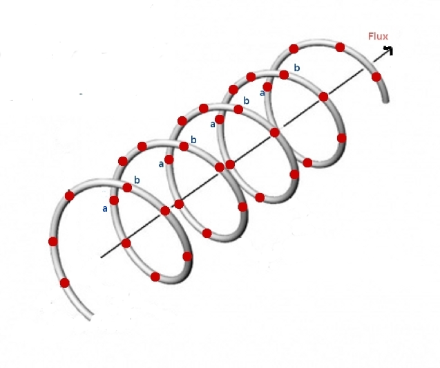
Figure 1: (Color online). A single handed helical conductor represented by a set of non-planar rings connected by some vertical bonds where each ring is formed by introducing a finite hopping due to close proximity of the atomic sites $a$ and $b$. A net circulating current is obtained in presence of AB flux $\phi$ passing through centers of individual rings.

is two-fold. (i) To investigate the interplay between conformational change and Hubbard correlation, which is still unaddressed, on circular current in a helical geometry. (ii) The helical geometry has recently become truly significant in understanding electron transport in several bio-molecules bio1 ; bio2 ; bio3 ; bio4 . Studying the behavior of circular current in presence of AB flux, conducting nature of such helical-like geometries can be estimated up to a certain level. We strongly believe that the present investigation may be helpful in analyzing magnetotransport in several real as well as artificially designed bio-molecules bio1 ; bio2 ; bio3 ; bio4 .

Using a tight-binding (TB) framework we describe the model and compute all the numerical results within a Hartree-Fock (HF) mean field level mf1 ; mf2 ; mf3 ; mf4 . The results are impressive. (i) By stretching and compressing the helical geometry we can control persistent current, keeping all the other physical parameters unchanged. This is quite different from the conventional cases, where current amplitude is regulated either by changing disorderness or by means of electron filling or something else. Thus, our system can be exploited to design conformation dependent current controlled device at the nano-scale level. (ii) The other important observation is that the geometry exhibits both $\phi_{0}/2$ and $\phi_{0}$ periodic persistent currents, while conventional AB rings provide only $\phi_{0}$ periodic currents.

The rest of the work is organized as follows. In Section II, we illustrate the model and give a detailed theoretical description to calculate circulating current within a Hartree-Fock MF approach. The results are analyzed in Section III which includes the effects of compression and extension of the conductor, Hubbard correlation, electron filling, etc. Finally, In Section IV we summarize our findings and present the future perspective.

II Model and Theoretical Framework

II.1 Model

Let us begin by referring to Fig. 1 where a single handed helical conductor in presence of magnetic flux $\phi$,

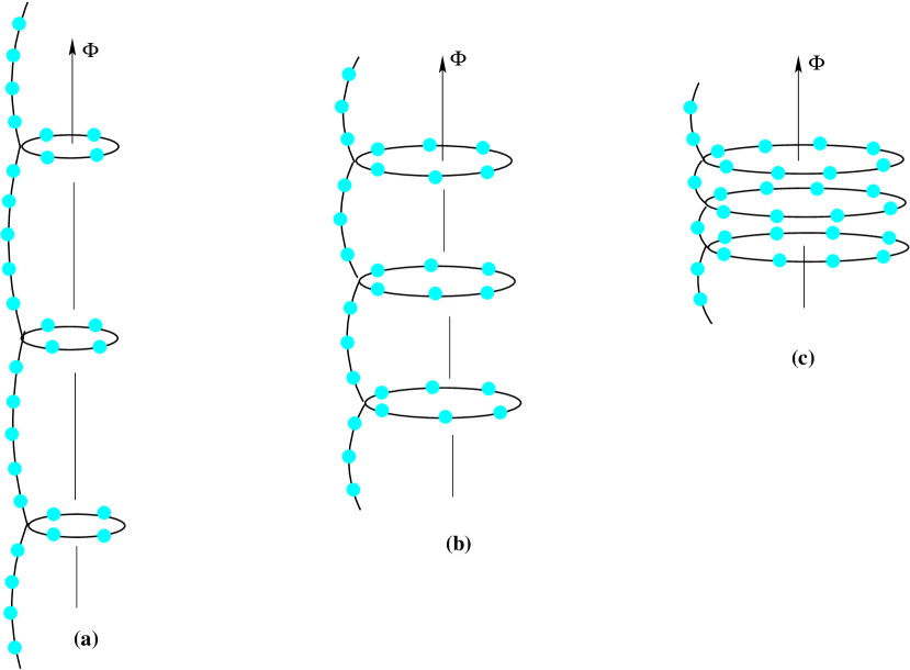
Figure 2: (Color online). Schematic view of a helical conductor in presence of magnetic flux $\phi$ under (a) stretched, (b) undeformed and (c) compressed conditions.

measured in unit of the elementary flux-quantum $\phi_{0}$ ($=ch/e$), is given. Here we consider three different cases, viz, stretched, undeformed and compressed, of the conductor depending on its configuration to explore conformation dependent magnetotransport properties. These configurations are schematically shown in Figs. 2(a), (b) and (c), respectively, where the conformational change is described by increasing and/or decreasing the ring size and chain length such that the total number of atomic sites $N$ of the helical conductor is fixed. It is written as $N=R\,n_{r}+Wn_{w}^{\mbox{\tiny in}}+n_{w}^{\mbox{\tiny out1}}+n_{w}^{\mbox{\tiny out2}}$, where $R$ corresponds to the total number of rings in which each ring contains $n_{r}$ atomic sites. The wire is divided into three parts. One is called intermediate wire that connects two adjacent rings and the other two are called outer wires. The parameter $W$ represents total number of intermediate wires in the conductor where each of these wires holds $n_{w}^{\mbox{\tiny in}}$ atomic sites, while $n_{w}^{\mbox{\tiny out1}}$ and $n_{w}^{\mbox{\tiny out2}}$ give the atomic sites in the two outer wires, respectively.

The TB Hamiltonian of such a helical conductor can be written as a sum of four terms like $H=H_{R}+H_{W}+H_{W}^{\mbox{\tiny out1}}+H_{W}^{\mbox{\tiny out2}}$, where they correspond to four different regions of the interacting conductor. These terms are described as follows. The Hamiltonian $H_{R}$ is given by $\sum_{R}H_{\mbox{\tiny ring}}$ where $H_{\mbox{\tiny ring}}$ describes identical rings, and, for any such rings it becomes,

$$H_{\mbox{\tiny ring}} = \sum_{\begin{subarray}{c}i=1\\ \sigma\end{subarray}}^{n_{r}}\epsilon_{i\sigma}^{r}c_{i\sigma}^{r\dagger}c_{i\sigma}^{r}+\sum_{\begin{subarray}{c}i=1\\ \sigma\end{subarray}}^{n_{r}-1}t\left[e^{i\theta}c_{i\sigma}^{r\dagger}c_{i+1\sigma}^{r}+h.c.\right]$$

$$+ \lambda\sum_{\sigma}\left[e^{i\theta}c_{n_{r}\sigma}^{r\dagger}c_{1\sigma}^{r}+h.c.\right]+U\sum_{i=1}^{n_{r}}c_{i\uparrow}^{r\dagger}c_{i\uparrow}^{r}c_{i\downarrow}^{r\dagger}c_{i\downarrow}^{r}.$$

Here, $\epsilon_{i\sigma}^{r}$ is the site energy of an electron at $i$th site of spin $\sigma$ ($\uparrow$, $\downarrow$), $c_{i\sigma}^{r\dagger}$ and $c_{i\sigma}^{r}$ are the creation and annihilation operators, respectively. $t$ represents the nearest-neighbor hopping integral and $\theta$ ($=2\pi\phi/n_{r}\phi_{0}$) is the phase factor associated with magnetic flux $\phi$. $\lambda$ measures non-zero hopping between the atomic sites $a$ and $b$ (see Fig. 1) due to their close proximity and $U$ gives the on-site Coulomb interaction.

In a similar fashion we express $H_{W}$ ($=\sum_{W}H_{\mbox{\tiny wire}}^{\mbox{\tiny in}}$) which describes the Hamiltonian of all inner wires, and for any such wires it gets the form,

$$H_{\mbox{\tiny wire}}^{\mbox{\tiny in}} = \sum_{\begin{subarray}{c}i=1\\ \sigma\end{subarray}}^{n_{w}^{\mbox{\tiny in}}}\epsilon_{i\sigma}^{w}c_{i\sigma}^{w\dagger}c_{i\sigma}^{w}+\sum_{\begin{subarray}{c}i=1\\ \sigma\end{subarray}}^{n_{w}^{\mbox{\tiny in}}-1}v\left[c_{i\sigma}^{w\dagger}c_{i+1\sigma}^{w}+h.c.\right]$$ (2)

$$+U\sum_{i=1}^{n_{w}^{\mbox{\tiny in}}}c_{i\uparrow}^{w\dagger}c_{i\uparrow}^{w}c_{i\downarrow}^{w\dagger}c_{i\downarrow}^{w}.$$

where, $v$ corresponds to the nearest-neighbor hopping integral and other parameters carry similar meaning like above.

Finally, to describe TB Hamiltonians $H_{W}^{\mbox{\tiny out1}}$ and $H_{W}^{\mbox{\tiny out2}}$ for the two outer arms we use exactly similar kind of TB Hamiltonian as given in Eq. 2, except that in one case $n_{w}^{\mbox{\tiny in}}$ is replaced by $n_{w}^{\mbox{\tiny out1}}$, while in the other case $n_{w}^{\mbox{\tiny in}}$ is substituted by $n_{w}^{\mbox{\tiny out2}}$. Both these outer and inner wires are coupled to the rings via the same hopping integral $v$.

This is the complete description of the model quantum system considered in this work, and, now we describe the Hartree Fock mean field scheme to evaluate ground state energy and finally to determine persistent current as a function of flux $\phi$.

II.2 Mean field approach

To evaluate energy eigenvalues of the interacting helical conductor we use generalized Hartree-Fock mean field approach mf1 ; mf2 ; mf3 ; mf4 where we decouple the interacting Hamiltonian into the non-interacting ones such that one is associated with up spin electrons and the other is related to down spin electrons. In this prescription on-site energies get modified and they are expressed as:

$$\epsilon_{i\uparrow}^{r(w)\prime} =\epsilon_{i\uparrow}^{r(w)}+U\langle n_{i\downarrow}^{r(w)}\rangle$$ (3a)

$$\epsilon_{i\downarrow}^{r(w)\prime} =\epsilon_{i\downarrow}^{r(w)}+U\langle n_{i\uparrow}^{r(w)}\rangle.$$ (3b)

Here, $n_{i\sigma}^{r(w)}=c_{i\sigma}^{r(w)\dagger}c_{i\sigma}^{r(w)}$ is the number operator and $r$ and $w$ are used to relate the ring and wire, respectively. With these modified on-site energies we can express the Hamiltonians of the ring as well as connecting wires in the decoupled form under mean field approximation as follows.

$$H_{\mbox{\tiny ring}}^{\mbox{\tiny MF}} = \sum_{i=1}^{n_{r}}\epsilon_{i\uparrow}^{r\prime}n_{i\uparrow}^{r}+\sum_{i=1}^{n_{r}-1}t\left[e^{i\theta}c_{i\uparrow}^{r\dagger}c_{i+1\uparrow}^{r}+h.c.\right]$$ (4)

$$+ \lambda\left[e^{i\theta}c_{n_{r}\uparrow}^{r\dagger}c_{1\uparrow}^{r}+h.c.\right]$$

$$+ \sum_{i=1}^{n_{r}}\epsilon_{i\downarrow}^{r\prime}n_{i\downarrow}^{r}+\sum_{i=1}^{n_{r}-1}t\left[e^{i\theta}c_{i\downarrow}^{r\dagger}c_{i+1\downarrow}^{r}+h.c.\right]$$

$$+ \lambda\left[e^{i\theta}c_{n_{r}\downarrow}^{r\dagger}c_{1\downarrow}^{r}+h.c.\right]$$

$$- \sum_{i=1}^{n_{r}}U\langle n_{i\uparrow}^{r}\rangle\langle n_{i\downarrow}^{r}\rangle$$

$$= H_{\mbox{\tiny ring}\uparrow}+H_{\mbox{\tiny ring}\downarrow}-\sum_{i=1}^{n_{r}}U\langle n_{i\uparrow}^{r}\rangle\langle n_{i\downarrow}^{r}\rangle$$

where $H_{\mbox{\tiny ring}\uparrow}$ describes the effective TB Hamiltonian for up spin electrons and for down spin electrons it is expressed by $H_{\mbox{\tiny ring}\downarrow}$. The term $\sum_{i=1}^{n_{r}}U\langle n_{i\uparrow}^{r}\rangle\langle n_{i\downarrow}^{r}\rangle$ is the constant term and it produces an energy shift.

Similar to Eq. 4 we can write the TB Hamiltonian of the inner wires as,

$$H_{\mbox{\tiny wire}}^{\mbox{\tiny in, MF}} = \sum_{i=1}^{n_{w}^{\mbox{\tiny in}}}\epsilon_{i\uparrow}^{w}n_{i\uparrow}^{w}+\sum_{i=1}^{n_{w}^{\mbox{\tiny in}}-1}v\left[c_{i\uparrow}^{w\dagger}c_{i+1\uparrow}^{w}+h.c.\right]$$ (5)

$$+ \sum_{i=1}^{n_{w}^{\mbox{\tiny in}}}\epsilon_{i\downarrow}^{w}n_{i\downarrow}^{w}+\sum_{i=1}^{n_{w}^{\mbox{\tiny in}}-1}v\left[c_{i\downarrow}^{w\dagger}c_{i+1\downarrow}^{w}+h.c.\right]$$

$$- \sum_{i=1}^{n_{w}^{\mbox{\tiny in}}}\langle n_{i\uparrow}^{w}\rangle\langle n_{i\downarrow}^{w}\rangle$$

$$= H_{\mbox{\tiny wire}\uparrow}+H_{\mbox{\tiny wire}\downarrow}-\sum_{i=1}^{n_{w}^{\mbox{\tiny in}}}U\langle n_{i\uparrow}^{w}\rangle\langle n_{i\downarrow}^{w}\rangle$$

where different terms have their usual meanings.

Exact expression like Eq. 5 also goes to the two outer arms with appropriate upper limits of the summation index as described before.

Combining all these decoupled Hamiltonians for different sub-parts we can write the effective Hamiltonian for the full interacting conductor in a general way, for the sake of simplification, as

$$H^{\mbox{\tiny MF}} = H_{\uparrow}+H_{\downarrow}-\sum_{i}U\langle n_{i\uparrow}\rangle\langle n_{i\downarrow}\rangle.$$ (6)

Now we can go through self-consistent procedure with these decoupled Hamiltonians setting initial guess values of $\langle N_{i\uparrow}\rangle$ and $\langle N_{i\downarrow}\rangle$. First we construct $H_{\uparrow}$ and $H_{\downarrow}$ considering these $\langle N_{i\uparrow}\rangle$ and $\langle N_{i\downarrow}\rangle$ and then diagonalize these Hamiltonians to find new set of $\langle N_{i\uparrow}\rangle$ and $\langle N_{i\downarrow}\rangle$. Again we repeat this procedure and continue it until a self-consistent solution is obtained. This is the most crucial step for mean-field scheme, and therefore, special emphasis should be given to choose the initial guess values of $\langle N_{i\uparrow}\rangle$ and $\langle N_{i\downarrow}\rangle$.

Once we get the self-consistent solution, the ground state energy of the system can be easily determined. At absolute zero temperature ($T=0\,$K) it becomes,

$$E_{g}=\sum_{p}E_{p\uparrow}+\sum_{p}E_{p\downarrow}-\sum_{i}U\langle n_{i\uparrow}\rangle\langle n_{i\downarrow}\rangle$$ (7)

where the summation is taken upto the Fermi energy $E_{F}$. $E_{p\uparrow}$’s and $E_{p\downarrow}$’s are the eigenvalues of the sub-Hamiltonians for up and down spin electrons, respectively.

Finally, we determine persistent current of the helical conductor, at absolute zero temperature, from the relation gefen ; pc1 ,

$$I(\phi)=-\frac{\partial E_{g}(\phi)}{\partial\phi}$$ (8)

where, $E_{g}(\phi)$ is the ground state energy in presence of flux $\phi$ which is determined by summing over lowest $N_{e}$ energy levels. $N_{e}$ represents the electron filling.

III Numerical results and discussion

Now, we present the results which are computed numerically based on the above theoretical prescription (discussed in Sec. II). The common parameters for our calculations, unless stated otherwise, are: $\epsilon_{i\uparrow}^{r}=\epsilon_{i\downarrow}^{r}=\epsilon_{i\uparrow}^{w}=\epsilon_{i\downarrow}^{w}=0$, $t=1\,$eV, $v=1\,$eV and $T=0\,$K. Throughout the analysis we measure the energy in unit of $t$ and current in unit of $et/h$. Here, we essentially focus on the variation of conformation dependent circular current in a helical conductor in presence of magnetic flux $\phi$. Before addressing this issue, first we describe the nature of energy-flux characteristics to make the present work a self-contained study.

In Fig. 3 we show the variation of ground state energy $E_{g}$ as a function of magnetic flux $\phi$ for a helical conductor considering its three different configurations, viz, undeformed, stretched and compressed. Two different band fillings are considered to compute the ground state

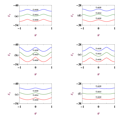
Figure 3: (Color online). $E_{g}$-$\phi$ characteristics of a helical conductor with $N=39$ (considering $R=4$ and $W=3$) for its different conformations where the left column corresponds to the half-filled band case i.e., $N_{e}=39$, while the other column represents $N_{e}=19$. The first row describes the undeformed conductor where we set $n_{w}^{\mbox{\tiny out1}}=n_{w}^{\mbox{\tiny out2}}=3$, $n_{r}=6$ and $n_{w}^{\mbox{\tiny in}}=3$. For the second row the results are shown for the stretched conductor where we choose $n_{w}^{\mbox{\tiny out1}}=n_{w}^{\mbox{\tiny out2}}=4$, $n_{r}=4$ and $n_{w}^{\mbox{\tiny in}}=5$. Finally, the last row represents the compressed conductor with the parameters $n_{w}^{\mbox{\tiny out1}}=n_{w}^{\mbox{\tiny out2}}=2$, $n_{r}=8$ and $n_{w}^{\mbox{\tiny in}}=1$. In each of these spectra $E_{g}$ is computed for three different values of $U$ as shown by three distinct colored curves, considering $\lambda=1\,$eV.

energies and they are presented in two different columns. For the first column we set $N_{e}=39$, while it is $19$ for the other column and in all these cases we determine $E_{g}$ considering three different values of $U$ to investigate the interplay between conformational change and on-site Hubbard correlation. In this particular conductor we choose $N=39$ and it is distributed among four rings ($R=4$) and three internal wires ($W=3$) including two outer wires in appropriate numbers to get three distinct configurations of the helical conductor. Comparing the spectra given in Fig. 3 it is observed that the ground state energy exhibits maximum variation with flux $\phi$ for the stretched configuration, irrespective of $U$ as well as band fillings ($2$nd row of Fig. 3) and it becomes much flatter as we move towards the compressed one. This essentially leads to maximum circular current in the stretched case, while lesser currents are obtained in other two cases, which are described later in Fig. 4, since current is determined by taking the first order derivative of $E_{g}$ with respect to flux $\phi$ (see Eq. 8). With this conformation dependent variation it is also important to note that the ground state energy significantly increases with the rise of $U$ and the slope of $E_{g}$-$\phi$ curve changes in a large and/or small scale depending on the band filling, and it (change in slope) becomes much clearly seen from current-flux characteristics rather than $E_{g}$-$\phi$ spectra. All these ground state energies exhibit $\phi_{0}$ flux-quantum periodicity.

In Fig. 4 we present the variation of persistent current

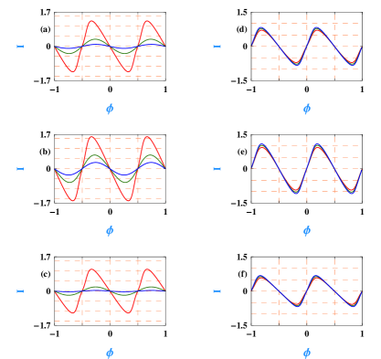
Figure 4: (Color online). $I$-$\phi$ characteristics of a helical conductor with $N=190$ (considering $R=4$ and $W=3$) and $\lambda=1\,$eV for its different conformations where the left column corresponds to the half-filled band case i.e., $N_{e}=190$, while the other column represents $N_{e}=95$. The three different rows represent the results for the three separate conformations as prescribed in Fig. 3. In the first row we set $n_{w}^{\mbox{\tiny out1}}=n_{w}^{\mbox{\tiny out2}}=14$, $n_{r}=30$ and $n_{w}^{\mbox{\tiny in}}=14$, while for the second row the parameters are $n_{w}^{\mbox{\tiny out1}}=n_{w}^{\mbox{\tiny out2}}=18$, $n_{r}=22$ and $n_{w}^{\mbox{\tiny in}}=22$. Finally, in the last row we consider $n_{w}^{\mbox{\tiny out1}}=n_{w}^{\mbox{\tiny out2}}=10$, $n_{r}=38$ and $n_{w}^{\mbox{\tiny in}}=6$. In each of these spectra $I$ is computed for three different values of $U$, shown by three distinct colored curves, where the red, green and blue lines in the left column correspond to $U=0$, $0.5$ and $1$, respectively, and they are $0$, $1$ and $2$, respectively, for the right column.

$I$ as a function of flux for a typical helical conductor with $N=190$ considering different values of $U$ for two distinct band fillings. In the first column the currents are shown for $N_{e}=190$, while in the second column we compute the currents setting $N_{e}=95$. The results are noteworthy. It is observed that the current becomes maximum for the stretched geometry and it gradually decreases as we increase the size of the ring i.e., when we move towards the compressed one. This behavior is independent of the band filling as well as the Hubbard interaction strength. The signature of higher current for the stretched conductor and smaller current for the other two configurations can be clearly understood from the variation of energy-flux characteristics discussed above. In addition it is also important to note that for the half-filled band case ($N_{e}=190$) the current changes sharply with increasing $U$, while away from half-filling ($N-e=95$) it becomes less sensitive to $U$. In all these cases current provides $\phi_{0}$ flux-quantum periodicity.

The results discussed so far, viz, $E_{g}$-$\phi$ and $I$-$\phi$ spectra, are computed for some typical helical conductors where the number of

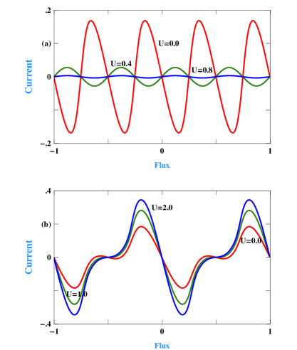
Figure 5: (Color online). Current-flux characteristics for a helical conductor with $N=190$ (considering $R=4$ and $W=3$) and $\lambda=1\,$eV in (a) half-filled ($N_{e}=190$) and (b) quarter-filled ($N_{e}=95$) cases. The other physical parameters are: $n_{w}^{\mbox{\tiny out1}}=14$, $n_{w}^{\mbox{\tiny out2}}=15$, $n_{r}=29$ and $n_{w}^{\mbox{\tiny in}}=15$.

atomic sites $n_{r}$ in each ring is even. Now, to check if any anomalous behavior is observed in current-flux characteristics for odd $n_{r}$, in Fig. 5 we present the results of persistent currents considering helical conductor with $n_{r}=29$ (odd $n_{r}$). Two different cases are shown, where in (a) currents are determined for $N_{e}=190$ (half-filled), while in (b) they are computed when $N_{e}=95$ (quarter-filled). The results are quite interesting. For the half-filled band case current exhibits $\phi_{0}/2$ flux-quantum periodicity instead of the $\phi_{0}$ periodicity as obtained in conventional cases. This typical behavior is only observed for the half-filled band case with odd ring size, since the current regains its $\phi_{0}$ periodicity as long as the electron filling gets changed which is clearly observed by comparing the spectra given in Figs. 5(a) and (b). From our extensive numerical analysis we find that this $\phi_{0}/2$ periodicity is the generic feature of persistent current for odd $n_{r}$ in the half-filled band case, though its physical argument is not clear at this stage and we hope it can be analyzed in our future work. Here, it is also significant to state that the current amplitude sharply decreases with $U$ for the half-filled case, while quite comparable currents are obtained for the other filling. In the limit of half-filling each atomic site is filled with an electron (up or down), and thus, it does not allow to hop an electron from one site to the other due to repulsive nature of $U$ which results reduced current with increasing $U$. While, for the system with less than half-filling there is always an empty site, and therefore, electron can hop into this empty site. The probability of electron hopping increases with lower value of $U$, but it tends to decrease when $U$ exceeds the critical limit yielding a smaller current. This critical value strongly depends on the system size and electron filling.

Finally, we discuss the proximity effect between the atomic sites $a$ and

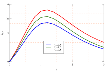
Figure 6: (Color online). Current amplitude at a typical magnetic flux $\phi=0.35$ for a helical conductor with $N=190$ (considering $R=4$ and $W=3$) as function of proximity integral $\lambda$ when $N_{e}$ is set at $160$. The other physical parameters are: $n_{w}^{\mbox{\tiny out1}}=n_{w}^{\mbox{\tiny out2}}=14$, $n_{r}=30$ and $n_{w}^{\mbox{\tiny in}}=14$.

$b$ on circular current. The results are presented in Fig. 6, where we show the variation of typical current amplitude as a function of hopping integral $\lambda$ setting $\phi=0.35$. For all three different values of $U$, we see that persistent current monotonically increases and after reaching the maximum at $\lambda=1\,$eV, it eventually decreases with $\lambda$. At this typical value of $\lambda$, the system behaves like a perfect one since we set $t=v=1\,$eV in our theoretical formulation, which results a maximum current. On the other hand for all other cases (when $\lambda\neq t$ and $v$) current decreases due to this anisotropy in the hopping integral. This anisotropy is directly related to the closeness of the atomic sites $a$ and $b$, and thus, tuning the proximity between these atomic sites we can regulate current amplitude which might be helpful in designing current controlled device at nano-scale level.

IV Conclusion

In the present work we investigate conformation dependent circular current in a single handed helical conductor in presence of AB flux $\phi$. A tight-binding framework is given to illustrate the model where electronic correlation is analyzed in the Hartree-Fock mean field level. Several important features are obtained from our numerical analysis those are summarized as follows. (i) Current amplitude can be controlled by stretching and compressing the geometry, keeping all other parameters unchanged. (ii) Both $\phi_{0}$ and $\phi_{0}/2$ flux-quantum periodicities are obtained in circular currents. The unconventional $\phi_{0}/2$ periodicity is observed only for the half-filled band case when the conductor contains rings with odd number of atomic sites. (iii) Circulating current can also be regulated by tuning the coupling parameter between the atomic sites $a$ and $b$. We believe that all the results studied here can be utilized to investigate magneto-transport in several bio-molecular systems having this helical like geometry.

In our analysis we compute the results for some typical parameter values of on-site energies, hopping integrals, system size, etc., but all these features remain unchanged for any other set of parameter values which certainly demands an experimental verification towards this direction. The other valid approximation is the zero temperature limit, though finite temperature extension of our analysis is a very simple task. The crucial point is that the physical properties studied above are not affected as long as the average level spacing $\Delta E$ is greater than $k_{B}T$. For our geometry we can safely reach upto a sub-Kelvin temperature limit.

References

- (1) M. Büttiker, Y. Imry, and R. Landauer, Phys. Lett. A 96, 365 (1983).
- (2) H. F. Cheung, Y. Gefen, E. K. Reidel, and W. H. Shih, Phys. Rev. B 37, 6050 (1988).
- (3) V. Ambegaokar and U. Eckern, Phys. Rev. Lett. 65, 381 (1990).
- (4) A. Schmid, Phys. Rev. Lett. 66, 80 (1991).
- (5) U. Eckern and A. Schmid, Europhys. Lett. 18, 457 (1992).
- (6) H. Bary-Soroker, O. Entin-Wohlman, and Y. Imry, Phys. Rev. B 82, 144202 (2010).
- (7) W. Rabaud, L. Saminadayar, D. Mailly, K. Hasselbach, A. Benoit, and B. Etienne, Phys. Rev. Lett. 86, 3124 (2001).
- (8) D. Mailly, C. Chapelier, and A. Benoit, Phys. Rev. Lett. 70, 2020 (1993).
- (9) R. A. Smith and V. Ambegaokar, Europhys. Lett. 20, 161 (1992).
- (10) H. Bouchiat and G. Montambaux, J. Phys. (Paris) 60, 2695 (1989).
- (11) E. Gambetti-Césare, D. Weinmann, R. A. Jalabert, and Ph. Brune, Europhys. Lett. 60, 120 (2002).
- (12) S. K. Maiti, M. Dey, S. Sil, A. Chakrabarti, and S. N. Karmakar, Europhys. Lett. 95, 57008 (2011).
- (13) S. K. Maiti, Solid State Commun. 150, 2212 (2010).
- (14) S. K. Maiti, J. Chowdhury and S. N. Karmakar, Phys. Lett. A 332, 497 (2004).
- (15) S. K. Maiti, J. Appl. Phys. 110, 064306 (2011).
- (16) L. P. Lévy, G. Dolan, J. Dunsmuir, and H. Bouchiat, Phys. Rev. Lett. 64, 2074 (1990).
- (17) E. M. Q. Jariwala, P. Mohanty, M. B. Ketchen, and R. A. Webb, Phys. Rev. Lett. 86, 1594 (2001).
- (18) N. O. Birge, Science 326, 244 (2009).
- (19) V. Chandrasekhar, R. A. Webb, M. J. Brady, M. B. Ketchen, W. J. Gallagher, and A. Kleinsasser, Phys. Rev. Lett. 67, 3578 (1991).
- (20) H. Bluhm, N. C. Koshnick, J. A. Bert, M. E. Huber, and K. A. Moler, Phys. Rev. Lett. 102, 136802 (2009).
- (21) M. Iskin and I. O. Kulik, Phys. Rev. B 70, 195411 (2004).
- (22) E. H. M. Ferreira, M. C. Nemes, M. D. Sampaio, H. A. Weidenmüller, Phys. Lett. A 333, 146 (2004).
- (23) H. Mori and R. Ota, J. Phys.: Conf. Ser. 150, 022058 (2009).
- (24) S. K. Maiti, J. Comput. Theor. Nanosci. 6, 187 (2009).
- (25) R. Prince, S. Barnes, and J. Moore, J. Am. Chem. Soc. 122, 2758 (2000).
- (26) M. Inouye, M. Waki, and H. Abe, J. Am. Chem. Soc. 126, 2022 (2004).
- (27) T. Mizutani, S. Yagi, and H. Ogoshi, J. Org. Chem. 63, 8769 (1998).
- (28) Y. Kudo, T. Ohno, and Y. Ishimaru, J. Am. Chem. Soc. 123, 12700 (2001).
- (29) H. Kato and D. Yoshioka, Phys. Rev. B 50, 4943 (1994).
- (30) A. Kambili, C. J. Lambert, and J. H. Jefferson, Phys. Rev. B 60, 7684 (1999).
- (31) S. K. Maiti and A. Chakrabarti, Phys. Rev. B 82, 184201 (2010).
- (32) S. K. Maiti, Phys. Status Solidi B 248, 1933 (2011).
- (33) S. K. Maiti, J. Chowdhury and S. N. Karmakar, J. Phys.: Condens Matter 18, 5349 (2006).