Evaluation of entanglement measures by a single observable
Abstract
We present observable lower bounds for several bipartite entanglement measures including entanglement of formation, geometric measure of entanglement, concurrence, convex-roof extended negativity, and G-concurrence. The lower bounds facilitate estimates of these entanglement measures for arbitrary finite-dimensional bipartite states. Moreover, these lower bounds can be calculated analytically from the expectation value of a single observable. Based on our results, we use several real experimental measurement data to get lower bounds of entanglement measures for these experimentally realized states. In addition, we also study the relations between entanglement measures.
pacs:
03.67.-a, 03.65.Ta, 03.67.LxI Introduction
Quantum entanglement is widely recognized as a valuable resource in quantum information processing. However, it is far from simple to fully determine entanglement. Therefore, the characterization and quantification of entanglement become fundamental problems in quantum information theory. Lots of entanglement measures have been proposed, such as entanglement of formation, geometric measure of entanglement, concurrence, and convex-roof extended negativity.
Consider a finite dimensional bipartite system, one is subsystem and the other one is subsystem . The entanglement of formation (EOF) is the first entanglement measure built by the convex roof construction EOFde1 ; EOFde2 . For a pure state , it is defined by , where stands for the von Neumann entropy and is the reduced density matrix of subsystem . For a mixed state , the EOF is defined by the convex roof, for all possible ensemble realizations , where and . The infimum represents the minimal possible average entanglement over all pure state decompositions of . The geometric measure of entanglement (GME) is another kind of convex-roof entanglement measures GME1 ; GME2 . For an arbitrary bipartite pure state with being its Schmidt coefficients, the GME is defined by . Similarly, the GME is extended to mixed states by the convex roof. The concurrence was firstly introduced for two-qubit states by Ref. EOFde1 , and based on it Wootters and co-workers derived computable formulae for concurrence and EOF in the two-qubit case 2qubit1 ; 2qubit2 . After that, Refs. concurrence3 ; concurrence4 ; concurrence5 extended it to bipartite higher-dimensional systems, i.e., for pure states, and its convex roof for mixed states. The convex roof extended negativity (CREN) is generalized from the negativity, which is strongly related with the partial transpose ppt . For a bipartite state , its negativity reads negativity (for simplicity we ignore the coefficient ), where stands for the trace norm and is partial transpose with respect to subsystem . The positive negativity is a necessary and sufficient condition of entanglement for pure states, and mixed states, but only a sufficient condition for higher-dimensional mixed states ppt . To overcome this drawback, Lee et al. proposed the CREN CREN . For a pure state , CREN is defined by the negativity . For mixed states, CREN is defined by the convex roof. Last but not least, the G-concurrence can be defined by the determinant of the reduced density matrix: for an () pure state GME1 ; Gour ; Fan , and for mixed states, the G-concurrence is defined by the convex roof as well Uhlmann .
Although many entanglement measures have been proposed EOFde1 ; EOFde2 ; GME1 ; GME2 ; 2qubit1 ; 2qubit2 ; concurrence3 ; concurrence4 ; concurrence5 ; ppt ; negativity ; CREN ; Gour ; Fan ; Uhlmann , there are only a few explicit expressions of these measures for two-qubit states and some special kinds of higher-dimensional mixed states 2qubit2 ; eof1 ; GME2 ; iso3 ; werner ; CREN . Furthermore, for a general state it is proved that computing many entanglement measures including the entanglement of formation is NP-hard NP ; yichen , which implies that we could only derive bounds on (rather than compute exact values of) these entanglement measures. Thus, in order to evaluate entanglement measures, lower and upper bounds of entanglement measures for general higher-dimensional states and multipartite states have been proposed mintert04 ; bounds1 ; bounds2 ; bounds3 ; bounds4 ; bounds5 ; bounds6 ; bounds7 ; bounds8 ; bounds9 ; bounds10 ; bounds11 ; bounds12 ; bounds13 ; bounds14 ; ob2 ; bounds15 ; bounds16 . Besides, the lower bounds of entanglement measures can server as a valuable tool for optimal control cui . However, if the proposed bound cannot be directly measured in experiments, quantum state tomography has to be performed which leads to rapidly growing experimental resources as system size increases. Therefore, experimentally observable lower and upper bounds of entanglement measures attract much interest recently mintert ; guhne ; lower ; Huang ; zhang ; ob1 ; ob3 ; ob4 ; ob5 ; ob6 .
In this paper, we shall propose observable lower bounds for EOF, GME, concurrence, CREN, and G-concurrence in finite-dimensional bipartite systems. These lower bounds can be obtained from the expectation value of a single observable. Based on our results, we will present several examples using real experimental measurement data. Furthermore, the relations between entanglement measures will be studied.
II Entanglement of formation
For simplicity, we use the denotation . Here denotes the convex hull of the function , which is the largest convex function that is bounded above by the given function . The denotation has been used to get explicit expressions and bounds for the EOF eof1 ; eof2 ; eof3 ; svl2 ; eof4 ; eof5 ; werner .
Theorem 1.— For any () quantum state , its entanglement of formation satisfies
| (1) |
where , , , with being the standard binary entropy function, and being an arbitrary pure entangled state in system (where are its Schmidt coefficients in decreasing order). The convex hull of is
| (6) |
Proof.– We first find the minimal admissible for a given , where are eigenvalues of and is the Schmidt vector . Consider the following function,
| (7) |
As shown in Ref. eof1 , the minimal versus corresponds to in the form for . Therefore, one can get with .
Suppose that we have already found an optimal decomposition for to achieve the infimum of , then by definition. Since is a monotonously increasing convex function and satisfies for a given , one thus has
where with being its Schmidt coefficients in decreasing order, and we have used
| (8) | |||||
where the second inequality holds since the theorem shown in Ref. horn , and the detailed proof has been given in the appendix. Therefore,
| (9) | |||||
Together with , one can get . Since is a monotonously increasing function and , one has .
As introduced above, is the largest convex function that is bounded above by the given function . From the expression of , the explicit expression of is as Eq. (6) eof1 ; eof2 ; eof3 . Actually, the same function has been gotten for the EOF of isotropic states eof1 and the lower bound of EOF based on partial transpose and realignment criteria in Refs. eof2 ; eof3 .
III Geometric measure of entanglement
Similar to entanglement of formation, we can also find an observable lower bound for the GME.
Theorem 2.— For any () quantum state , its geometric measure of entanglement satisfies
| (10) |
where , with , and
| (11) |
Proof.— We first find the minimal admissible for a given , where . Consider the following function,
| (12) |
As shown in the appendix, the minimal versus corresponds to in the form for . Therefore, holds, with .
Similar to the proof of Theorem 1, suppose that we have already found an optimal decomposition for to achieve the infimum of , then by definition. Since is a monotonously increasing convex function and satisfies for a given , one thus has
where, similar to the proof of Theorem 1, we have used .
From the definition of , one can see , since is a convex function. The same function has been used for the GME of isotropic states GME2 .
IV Concurrence
In the following, we shall also present an observable lower bound for the concurrence.
Theorem 3.— For any () quantum state , its concurrence satisfies
| (13) |
where , with , , and
| (14) |
Proof.— Similarly, we first find the minimal admissible for a given . Consider the following function,
| (15) |
As shown in the appendix, the minimal versus corresponds to still in the form for . Therefore, holds, with .
Similar to the proofs of Theorem 1 and 2, suppose that we have already found an optimal decomposition for to achieve the infimum of , then by definition. Since is a monotonously increasing convex function and satisfies for a given , one thus has
where has been used again.
From the definition of co, one can get Eq. (14), since is a monotonously increasing concave function as shown in the appendix. The same function has been gotten for the concurrence of isotropic states iso3 , the lower bound of concurrence based on partial transpose and realignment criteria in Ref. kai , and the special case of Eq. (13) with being the maximally entangled state fef1 ; fef2 .
V Convex-roof extended negativity
Similarly, an observable lower bound of CREN has been presented as follows.
Theorem 4.— For any () quantum state , its convex-roof extended negativity satisfies
| (16) |
where .
Proof.— Similar to the proofs of the theorems above, suppose that we have already found an optimal decomposition for to achieve the infimum of , then by definition. It is worth noticing that, for an arbitrary pure state with being its Schmidt coefficients in decreasing order, we have . Thus,
where has been proved in Theorem 1. Actually, a similar function has been gotten for the CREN of isotropic states CREN .
VI G-concurrence
Last but not least, one can present an observable lower bound of G-concurrence as follows.
Theorem 5.— For any () quantum state , its G-concurrence satisfies
| (17) |
where , with , , , and
| (18) |
Proof.— Similarly, we first find the minimal admissible for a given . Consider the following function,
| (19) |
As shown in Ref. 201605 and the appendix, the minimal versus corresponds to in the form for . Therefore, holds, with and .
Similar to the proofs of above theorems, suppose that we have already found an optimal decomposition for to achieve the infimum of , then by definition. Since is a monotonously increasing convex function and satisfies for a given , one thus has
where has been used again.
From the definition of co, one can get Eq. (18), since is a monotonously increasing concave function in as shown in Ref. 201605 . The same function has been gotten for the G-concurrence of axisymmetric states 201605 , and the lower bound of G-concurrence for arbitrary states which is the special case of Eq. (17) with being the maximally entangled state 201605 .
Remark 1.— It is worth noticing that when we choose a special case for , i.e. where is the maximally entangled state, then becomes to and . For this special case, our results shown in all the above theorems can be proved in a different manner: for an arbitrary state , one can project it onto the isotropic states by the twirling operation, i.e. , which is a local operations and classical communication (LOCC) operation and therefore cannot increase entanglement. Moreover, we have , since it is invariant under the twirling operation. The entanglement measures of the isotropic states can be expressed as a function of eof1 ; GME2 ; iso3 ; CREN . Thus, one can get lower bounds of entanglement measures for from the entanglement measures of the isotropic states, this idea to get a lower bound has been known since the earliest paper EOFde1 . However, this alternative proof for is not valid for a general .
Remark 2.— From Theorem 1 to Theorem 5, all the lower bounds proposed above are the functions of , which only depends on the expectation value of a single observable . Therefore, it will be much easier to evaluate than tomography in experiments.
VII Examples and experimental measurements
The first example is a real experimental state shown in Ref. real . Tonolini et al. experimentally realized a high-dimensional two-photon entangled state, with dimension of each photon being equal to . They reconstructed the density matrix of the experimental state, and found the fidelity with the maximally entangled pure state being . Therefore, our parameter for this experimental state should be . Using Eqs. (1), (10), (13), and (16), one can arrive at
for this real experimental state.
The second example is also from a real experiment real2 . In Ref. real2 , the authors experimentally realized a special three-photon pure state: and a four-photon Dicke state with two exciations . The square of fidelities for the special state and the Dicke state are measured to be and , respectively. For simplicity, we only consider the entanglement under bipartition for the three-photon special state and bipartition for the four-photon Dicke state. Other bipartition entanglement can also be calculated analytically based on our theorems. Therefore, our parameters for these experimental states should be with and , and with and . Using Eqs. (1), (10), (13), and (16), one can arrive at
for these real experimental states.
In the first example shown above, Tonolini et al. used compressive sensing to reduce the number of measurements, and 2506 measurements are needed for state reconstruction. Actually, the whole state reconstruction is not necessary for our lower bounds. We only need to perform local measurements (or one global measurement) to obtain the expectation value of for dimensional states. If the global measurement is not easy to be performed in experiments, one can use local measurements instead of it. We recall a complete set of local orthogonal observables (LOOs) introduced in Ref. LOO , i.e., , where and . The LOOs satisfy the orthogonal condition , and the complete condition for an arbitrary observable . Thus, , where means transpose of which is another complete set of LOOs, and . Therefore, only local measurements are required which is much less than the number of measurements required by tomography. For the first example , we only need local measurements, much less than 2506 measurements needed by the compressive sensing. When , the expression of has been widely known from Ref. nielsen . Moreover, Ref. namiki proposed methods to get a lower bound of the maximally entangled fraction with a rather smaller number of local measurements.
VIII Relations between entanglement measures
There have been comparative studies of entanglement measures. Horodecki et al. introduced axiomatic approach for entanglement measures Horodecki . Eltschka et al. proposed inequalities between the concurrence and CREN for any () quantum state fef2 , . We shall study the relations between concurrence, geometric measure of entanglement and CREN.
Theorem 6.— For any () quantum state , its concurrence , geometric measure of entanglement , and convex-roof extended negativity satisfy
| (20) | |||
| (21) | |||
| (22) |
where with and the integer , , .
Proof.— Let be the optimal ensemble for and be the Schmidt coefficients in decreasing order for . Thus,
since is a concave function and we have used the fact that .
In order to prove Eq. (21), the properties of are needed: is a decreasing function, i.e., if , and . Therefore, from Eq. (20) we have , which is equivalent to Eq. (21).
It is worth noticing that where . Thus, holds. Together with , we have . Therefore,
holds, and since we get Eq. (22).
IX Discussion and conclusion
Actually, the method we used to get lower bounds of EOF, GME, concurrence, CREN and G-concurrence can be generalized to arbitrary bipartite convex-roof entanglement measures. Suppose that the entanglement measure on an () pure state is , where is the Schmidt vector. We first get the minimal admissible for a given , i.e., . Thus, for a general () state , the lower bound of this entanglement measure is given by with , if the final function is a monotonously increasing convex function with respect to .
Our paper actually provided lower bounds on a variety of bipartite entanglement measures from a well-known entanglement witness exp1 :
| (23) |
where is an arbitrary pure entangled state in system (with being its Schmidt coefficients in decreasing order). This entanglement witness has been measured in many experiments, such as Refs. exp1 ; exp2 ; exp3 ; exp4 ; exp5 ; exp6 ; exp7 ; exp8 . Using this entanglement witness (where can be an arbitrary pure entangled state rather than only a maximally entangled state), one can obtain lower bounds on a variety of bipartite entanglement measures based on our method.
In conclusion, we present observable lower bounds for several entanglement measures defined by convex roof, which include EOF, GME, concurrence, CREN, and G-concurrence. The lower bounds estimate these entanglement measures for arbitrary finite-dimensional bipartite states. Moreover, these lower bounds can be easily obtained from the expectation value of a single observable. Based on our results, we present some examples using real experimental measurement data. In principle, our method can be used for arbitrary finite-dimensional bipartite convex-roof entanglement measures. Last but not least, the relations between entanglement measures are studied.
ACKNOWLEDGMENTS
This work is funded by the Singapore Ministry of Education (partly through the Academic Research Fund Tier 3 MOE2012-T3-1-009), the National Research Foundation, Singapore (Grant No. WBS: R-710-000-008-271), the financial support from RGC of Hong Kong(Grant No. 538213), the National Natural Science Foundation of China (Grants No. 11504253 and No. 11575155), and the startup funding from Soochow University (Grant No. Q410800215).
APPENDIX
Here we provide some details of calculations to get the expressions of , , , , , , and . The main idea is to calculate lower bounds of entanglement measures as a function of for pure states, and then to extend the bounds to mixed states by convex hull. The details of proving the inequality have also been presented.
IX.1 Calculation of and
In the following, we shall seek the minimal for a given . We use to denote the minimal for a given , i.e.,
| (S1) |
As shown in Ref. eof1 , the minimal versus corresponds to in the form
| (S2) |
with copies of and one copy of . Therefore, the minimal and corresponding are
| (S3) | |||||
| (S4) |
In order to show the minimal versus , we need the inverse function of . After some algebra, one can arrive at
| (S5) |
with . Substituting Eq. (S5) into Eq. (S3), we can get the expression for .
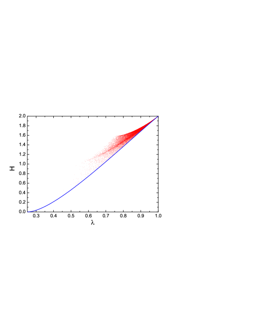
We can simulate the lower boundary of the region in versus plane. 50000 dots for randomly generated states with are displayed in Fig. 1. The lower boundary corresponds to . It is defined that is the largest convex function that is bounded above by the given function . From the expression of , the explicit expression of is obtained in Refs. eof1 ; eof2 ; eof3 , which is Eq. (2) shown in the main text.
IX.2 Calculation of and
We first seek the minimal for a given , where . We use to denote the minimal for a given , i.e.,
| (S6) |
It is interesting that, similar to , the minimal versus corresponds to in the form
| (S7) |
with copies of and one copy of . Therefore, the minimal and corresponding are
| (S8) | |||||
| (S9) |
where , since with . In order to show the minimal versus , we need the inverse function of . After some algebra, one can see that
| (S10) |
with . Substituting Eq. (S10) into Eq. (S8), we can get the expression for , i.e.,
| (S11) |
From Eq. (S11), we can find that
when . Thus, is a monotonously increasing function. Moreover, from the definition of , one can see that , since is a convex function. In order to prove this, we only need to show that . From Eq. (S11), one can get
| (S12) |
since is an integer () and . Therefore, , which is a monotonously increasing convex function.
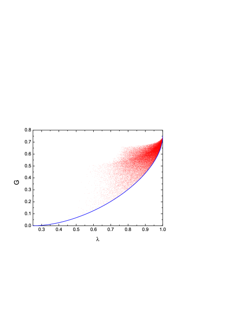
We can simulate the lower boundary of the region in versus plane. In Fig. 2, 50000 dots for randomly generated states with are displayed. The lower boundary corresponds to , which coincides with .
IX.3 Calculation of and
We first seek the minimal for a given . We use to denote the minimal for a given , i.e.,
| (S13) |
It is interesting that, similar to and , the minimal versus corresponds to in the form
| (S14) |
with copies of and one copy of . Therefore, the minimal and corresponding are
| (S15) | |||||
| (S16) |
In order to show the minimal versus , we need the inverse function of . After some algebra, one can arrive at
| (S17) |
with . Substituting Eq. (S17) into Eq. (S15), we can get the expression for , i.e.,
| (S18) | |||||
| (S19) |
From Eqs. (S18) and (S19), we can find that
| (S20) |
where
| (S21) | |||||
| (S22) | |||||
since and . Therefore,
| (S23) |
which means is a monotonously increasing function.
Furthermore, in order to show is a concave function, we need to prove that . One can use
| (S24) |
and
| (S25) | |||||
| (S26) |
Thus,
where
| (S27) | |||||
| (S28) | |||||
| (S29) | |||||
| (S30) |
with . It is easy to see that
| (S31) |
when . Thus,
| (S32) |
when , , and . Therefore, the convex hull of will be
| (S33) |
which is a straight line from to .
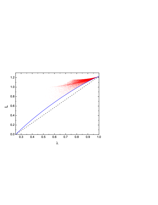
We can simulate the lower boundary of the region in versus plane. 50000 dots for randomly generated states with are displayed in Fig. 3. The lower boundary corresponds to , and the dashed black line corresponds to .
IX.4 Calculation of and
We first seek the minimal for a given . We use to denote the minimal for a given , i.e.,
| (S34) |
As shown in Ref. 201605 , the minimal versus corresponds to in the form
| (S35) |
with copies of and one copy of . Therefore, the minimal and corresponding are
| (S36) | |||||
| (S37) |
In order to show the minimal versus , we need the inverse function of . After some algebra, one can arrive at
| (S38) |
with . Substituting Eq. (S38) into Eq. (S36), we can get the expression for , i.e.,
| (S39) | |||||
| (S40) |
From Ref. 201605 , one can see that is a monotonously increasing concave function in . Therefore, the convex hull of will be
| (S41) |
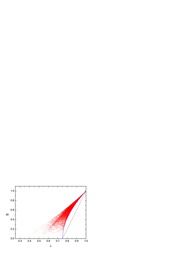
We can simulate the lower boundary of the region in versus plane. 50000 dots for randomly generated states with are displayed in Fig. 4. The lower boundary corresponds to , and the dashed black line corresponds to .
IX.5 Proof of the inequality
Here we give the details of proving . For any () quantum state , suppose that we have found an optimal decomposition for to achieve the infimum of , where is one kind of entanglement measure defined by the convex roof. For each , we have the expression
with being its Schmidt coefficients in decreasing order, where () is an () unitary matrix and is an matrix defined by . Similarly, for an arbitrary pure entangled given state in system, we have the expression
| (S42) |
where are its Schmidt coefficients in decreasing order, () is an () unitary matrix, and is an matrix defined by . Therefore, the maximum under all possible (which is an unitary matrix) and (which is an unitary matrix) is
| (S43) | |||||
where is an unitary matrix defined by , is an unitary matrix defined by , and are singular values of in decreasing order. The first inequality holds since for arbitrary matrix , and the second inequality holds since the following theorem horn :
Let ( matrix) and ( matrix) be given, let , and denote the ordered singular values of , , and by , , and . Then
| (S44) |
Therefore,
| (S45) |
where the first inequality holds since . Thus,
| (S46) |
Together with , one can obtain .
References
- (1) C. H. Bennett, D. P. DiVincenzo, J. A. Smolin, and W. K. Wootters, Phys. Rev. A 54, 3824 (1996).
- (2) M. Horodecki, Quantum Inf. Comput. 1, 3 (2001); D. Bruß, J. Math. Phys. (N.Y.) 43, 4237 (2002); M. B. Plenio and S. Virmani, Quantum Inf. Comput. 7, 1 (2007); R. Horodecki, P. Horodecki, M. Horodecki and K. Horodecki, Rev. Mod. Phys. 81, 865, (2009); O. Gühne and G. Tóth, Phys. Rep. 474, 1 (2009).
- (3) H. Barnum and N. Linden, J. Phys. A 34, 6787 (2001).
- (4) T.-C. Wei and P. M. Goldbart, Phys. Rev. A 68, 042307 (2003); T.-C. Wei, J. B. Altepeter, P. M. Goldbart, and W. J. Munro, ibid. 70, 022322 (2004).
- (5) S. Hill and W. K. Wootters, Phys. Rev. Lett. 78, 5022 (1997).
- (6) W. K. Wootters, Phys. Rev. Lett. 80, 2245 (1998).
- (7) K. Audenaert, F. Verstraete, and B. De Moor, Phys. Rev. A 64, 052304 (2001).
- (8) P. Rungta, V. Buzek, C. M. Caves, M. Hillery, and G. J. Milburn, Phys. Rev. A 64, 042315 (2001).
- (9) P. Badziag, P. Deuar, M. Horodecki, P. Horodecki, and R. Horodecki, J. Mod. Opt. 49, 1289 (2002).
- (10) M. Horodecki, P. Horodecki, and R. Horodecki, Phys. Lett. A 223, 1 (1996); A. Peres, Phys. Rev. Lett. 77, 1413 (1996).
- (11) K. Życzkowski, , P. Horodecki, A. Sanpera, and M. Lewenstein, Phys. Rev. A 58, 883 (1998); G. Vidal, and R. F. Werner, ibid. 65, 032314 (2002).
- (12) S. Lee, D.-P. Chi, S.-D. Oh, and J. Kim, Phys. Rev. A 68, 062304 (2003).
- (13) G. Gour, Phys. Rev. A 71, 012318 (2005).
- (14) H. Fan, K. Matsumoto, and H. Imai, J. Phys. A 36, 4151 (2003); H. Barnum and N. Linden, J. Phys. A 34, 6787 (2001).
- (15) A. Uhlmann, Entropy, 12, 1799 (2010).
- (16) P. Rungta and C. M. Caves, Phys. Rev. A 67, 012307 (2003).
- (17) K. G. H. Vollbrecht and R. F. Werner, Phys. Rev. A 64, 062307 (2001).
- (18) B. M. Terhal and K. G. H. Vollbrecht, Phys. Rev. Lett. 85, 2625 (2000).
- (19) S. Gharibian, Quant. Inf. Comp. 10, 343 (2010).
- (20) Y. Huang, New J. Phys. 16, 033027 (2014).
- (21) F. Mintert, M. Kuś, and A. Buchleitner, Phys. Rev. Lett. 92, 167902 (2004).
- (22) Z. Ma and M. Bao, Phys. Rev. A 82, 034305 (2010).
- (23) X.-S. Li, X.-H. Gao, and S.-M. Fei, Phys. Rev. A 83, 034303 (2011).
- (24) M.-J. Zhao, X.-N. Zhu, S.-M. Fei, and X. Li-Jost, Phys. Rev. A 84, 062322 (2011).
- (25) A. Sabour and M. Jafarpour, Phys. Rev. A 85, 042323 (2012).
- (26) X.-N. Zhu, M.-J. Zhao, and S.-M. Fei, Phys. Rev. A 86, 022307 (2012).
- (27) C. Eltschka and J. Siewert, Phys. Rev. A 89, 022312 (2014).
- (28) S. Rodriques, N. Datta, and P. Love, Phys. Rev. A 90, 012340 (2014).
- (29) M. Roncaglia, A. Montorsi, and M. Genovese, Phys. Rev. A 90, 062303 (2014).
- (30) Z.-H. Chen, Z.-H. Ma, O. Gühne, and S. Severini, Phys. Rev. Lett. 109, 200503 (2012).
- (31) Y.-K. Bai, Y.-F. Xu, and Z.D. Wang, Phys. Rev. Lett. 113, 100503 (2014).
- (32) C. Zhang, S. Yu, Q. Chen, and C.H. Oh, Phys. Rev. Lett. 111, 190501 (2013).
- (33) F. Nicacio and M. C. de Oliveira, Phys. Rev. A 89, 012336 (2014).
- (34) L. E. Buchholz, T. Moroder, O. Gühne, Ann. Phys. (Berlin) 528, 278 (2016).
- (35) M. Huber, J. I. de Vicente, Phys. Rev. Lett. 110, 030501 (2013); M. Huber, M. Perarnau-Llobet, and J.I. de Vicente, Phys. Rev. A 88, 042328 (2013).
- (36) Z.-H. Ma et al., Phys. Rev. A 83, 062325 (2011).
- (37) O. Gühne and M. Seevinck, New J. Phys. 12, 053002 (2010).
- (38) M. Huber, F. Mintert, A. Gabriel, and B.C. Hiesmayr, Phys. Rev. Lett. 104, 210501 (2010).
- (39) J. Cui, F. Mintert, New J. Phys. 17, 093014 (2015).
- (40) S. P. Walborn et al., Nature (London) 440, 1022 (2006); S. P. Walborn, P. H. Souto Ribeiro, L. Davidovich, F. Mintert, and A. Buchleitner, Phys. Rev. A 75, 032338 (2007).
- (41) O. Gühne, M. Reimpell, and R. F. Werner, Phys. Rev. Lett. 98, 110502 (2007); ibid. Phys. Rev. A 77, 052317 (2008).
- (42) F. Mintert and A. Buchleitner, Phys. Rev. Lett. 98, 140505 (2007); L. Aolita, A. Buchleitner, and F. Mintert, Phys. Rev. A 78, 022308 (2008).
- (43) Y.-F. Huang et al., Phys. Rev. A 79, 052338 (2009).
- (44) C. Zhang, S. Yu, Q. Chen, and C. H. Oh, Phys. Rev. A 84, 052112 (2011).
- (45) Y.-C. Liang, T. Vértesi, and N. Brunner, Phys. Rev. A 83, 022108 (2011).
- (46) Z.-H. Chen, Z.-H. Ma, J.-L. Chen, and S. Severini, Phys. Rev. A 85, 062320 (2012).
- (47) J.-Y. Wu, H. Kampermann, D. Bruß, C. Klöckl, and M. Huber, Phys. Rev. A 86, 022319 (2012).
- (48) Y. Hong, T. Gao, and F. Yan, Phys. Rev. A 86, 062323 (2012).
- (49) W. Song, L. Chen, Z.-L. Cao, arXiv:1604.02783.
- (50) K. Chen, S. Albeverio, and S.-M. Fei, Phys. Rev. Lett. 95, 210501 (2005).
- (51) S. M. Fei and X. Li-Jost, Phys. Rev. A 73, 024302 (2006).
- (52) T.-C. Wei et al., Phys. Rev. A 67, 022110 (2003).
- (53) M. Li and S.-M. Fei, Phys. Rev. A 82, 044303 (2010).
- (54) X.-N. Zhu and S.-M. Fei, Phys. Rev. A 86, 054301 (2012).
- (55) R. Horn and C. Johnson, Topics in Matrix Analysis (Cambridge University Press, Cambridge, 1991), Theorem 3.3.4.
- (56) K. Chen, S. Albeverio, and S.-M. Fei, Phys. Rev. Lett. 95, 040504 (2005).
- (57) M.-J. Zhao, Z.-G. Li, S.-M. Fei, and Z.-X.Wang, J. Phys. A: Math. Theor. 43, 275203 (2010).
- (58) C. Eltschka, G. Tóth, and J. Siewert, Phys. Rev. A, 91, 032327 (2015).
- (59) G. Sentís, C. Eltschka, O. Gühne, M. Huber, and J. Siewert, arXiv:1605.09783v1.
- (60) F. Tonolini, S. Chan, M. Agnew, A. Lindsay, and J. Leach, Sci. Rep. 4, 6542 (2014).
- (61) C. Zhang, C.J. Zhang, Y.F. Huang, Z.B. Hou, B.H. Liu, C.F. Li, and G.C. Guo, to be submitted.
- (62) S. Yu and N.-L. Liu, Phys. Rev. Lett. 95, 150504 (2005).
- (63) M. A. Nielsen, Phys. Lett. A 303, 249 (2002).
- (64) R. Namiki and Y. Tokunaga, Phys. Rev. Lett. 108, 230503 (2012).
- (65) M. Horodecki, P. Horodecki, and R. Horodecki, Phys. Rev. Lett. 84, 2014 (2000).
- (66) M. Bourennane et al. Phys. Rev. Lett. 92, 087902 (2004).
- (67) N. Kiesel et al. Phys. Rev. Lett. 95, 210502 (2005).
- (68) C.-Y. Lu et al. Nature Physics 3, 91 (2007).
- (69) W.-B. Gao et al. Nature Physics, 6, 331 (2010).
- (70) Y. F. Huang et al. Nat. Commun. 2, 546 (2011).
- (71) X.-C. Yao et al. Nature Photonics 6, 225 (2012).
- (72) C. Zhang et al. Phys. Rev. Lett. 115, 260402 (2015).
- (73) X.-L. Wang et al. arXiv:1605.08547.