Effect of Fluctuations on the NMR Relaxation Beyond the Abrikosov Vortex State

Abstract

The effect of fluctuations on the nuclear magnetic resonance (NMR) relaxation rate $W=T_{1}^{-1}$ is studied in a complete phase diagram of a 2D superconductor above the upper critical field line $H_{\mathrm{c2}}(T)$ . In the region of relatively high temperatures and low magnetic fields, the relaxation rate $W$ is determined by two competing effects. The first one is its decrease in result of suppression of quasi-particle density of states (DOS) due to formation of fluctuation Cooper pairs (FCP). The second one is a specific, purely quantum, relaxation process of the Maki-Thompson (MT) type, which for low field leads to an increase of the relaxation rate. The latter describes particular fluctuation processes involving self-pairing of a single electron on self-intersecting trajectories of a size up to phase-breaking length $\ell_{\phi}$ which becomes possible due to an electron spin-flip scattering event at a nucleus. As a result, different scenarios with either growth or decrease of the NMR relaxation rate are possible upon approaching the normal metal – type-II superconductor transition. The character of fluctuations changes along the line $H_{\mathrm{c2}}(T)$ from the thermal long-wavelength type in weak magnetic fields to the clusters of rotating FCP in fields comparable to $H_{\mathrm{c2}}(0)$. We find that below the well-defined temperature $T^{\ast}_{0}\approx 0.6T_{\mathrm{c0}}$, the MT process becomes ineffective even in absence of intrinsic pair-breaking. The small scale of FCP rotations ($\xi_{\rm{xy}}$) in so high fields impedes formation of long ($\lesssim\ell_{\phi}$) self-intersecting trajectories, causing the corresponding relaxation mechanism to lose its efficiency. This reduces the effect of superconducting fluctuations in the domain of high fields and low temperatures to just the suppression of quasi-particle DOS, analogously to the Abrikosov vortex phase below the $H_{\mathrm{c2}}(T)$ line.

I Introduction

Nuclear magnetic resonant (NMR) spin-lattice relaxation is a result of nuclei-interactions with low frequency excitations available in the investigated systemSlichter (1990). This fact makes NMR a powerful tool for studying low-energy excitation dynamics in novel materialsRigamonti et al. (1998).

In the Abrikosov phase of the type-II superconductors, for magnetic fields well above the critical field $H_{\mathrm{c1}}$ but still below $H_{\mathrm{c2}}$, magnetic flux lines are separated by superconducting regions at distances of the order of the coherence length $\xi_{\rm{xy}}$. The low-energy excitations driving spin-lattice relaxation are the weighted average of the intra-vortex excitations and of the contribution from the inter-vortex regions, possibly connected by a spin diffusion processSlichter (1990). In the vortex liquid phase, flux line diffusion provides an additional possible relaxation mechanism (see Ref. [Corti et al., 1996] and references therein).

In a recent workGlatz et al. (2011a) the authors pointed out that a dynamic state with clusters of coherently rotating FCP is formed above the $H_{\mathrm{c2}}(T)$ line at low temperatures. It is therefore of special interest to study the effect of this fluctuation analogue of the vortex state on the magnetic field dependence of the relaxation rate near $H_{\mathrm{c2}}\left(T\right)$. Some preliminary experimental studies were performedLascialfari and Rigamonti (shed) by measuring the ${}^{11}B$ NMR relaxation rates in a single crystal of superconducting Y​Ni₂​B₂ (${T_{\mathrm{c0}}=15.3}$K in zero field). The authors discussed an anomalous peak in the NMR relaxation rate magnetic field dependence $W(H)$ at temperatures $2K$ and $4K$ in fields close to $H_{\mathrm{c2}}(T)$, which they tentatively attributed to quantum fluctuations of magnetic flux lines.

Superconducting fluctuations affect the NMR spin-lattice relaxation rate of superconductors in a wide range of magnetic fields and temperatures above the upper critical field line $H_{\mathrm{c2}}(T)$ [Maniv and Alexander, 1977; Kuboki and Fukuyama, 1989; Heym, 1992; Randeria and Varlamov, 1994; Eschrig et al., 1999; Mosconi et al., 2000; Carretta et al., 1996; Mitrović et al., 1999; Gorny et al., 1999; Mitrović et al., 2002; Prando et al., 2011]. First of all, they suppress the density of quasi-particle excitationsAbrahams et al. (1970); Di Castro et al. (1990), which enters quadratically into the NMR relaxation rate, and, as a consequence, they reduce $W$. Nevertheless, this is not the only way for fluctuations to influence nuclear relaxation. There exists another, purely quantum, relaxation process of the Maki-Thompson (MT) type which consists of the fluctuation self-pairing of a single electron on a self-intersecting trajectory due to an electron spin-flip scattering event at a particular nucleusManiv and Alexander (1977); Kuboki and Fukuyama (1989); Larkin and Varlamov (2005) (see Fig. 1). The latter process opens a new channel of NMR signal relaxation leading to the increase of $W$.

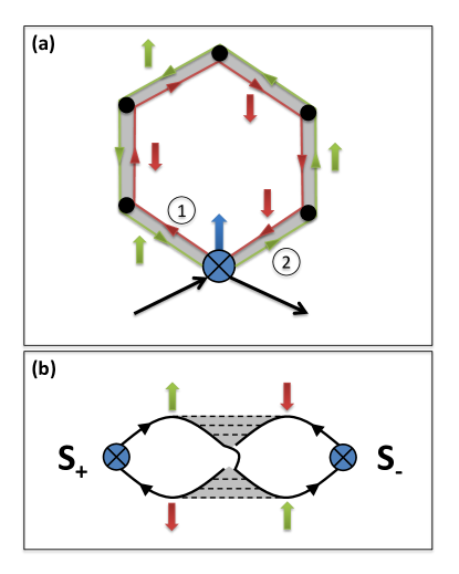
Figure 1: (Color online) The relaxation process of Maki-Thompson (MT) type related to the fluctuation pairing of electrons on self-intersecting trajectories involving their spin-flip scatterings on the investigated nuclei. (a) Initially electron moves along the trajectory 1 (clockwise, red), due to several impurity scattering events it returns to the departure point. In result of interaction with the nuclei, its spin and momentum flip and electron returns along almost the same trajectory 2 (counter-clockwise, green). During this motion it interacts with “itself in past” (corresponding superconducting interactions are shaded). Such process is possible due to “fast” motion of the electron along the trajectory and retarded character of electron-phonon interaction. (b) Representation of the same process as a Feynman diagram (compare with Fig. 2(c).

Below, intending to investigate first of all the region of the Abrikosov lattice formation from the side of normal metal, we study the effect of superconducting fluctuations both of the thermal and the quantum nature on the NMR relaxation mechanisms. We concentrate mainly on the most interesting case of a two-dimensional $s-$wave superconductor restricting our consideration by the representative dirty limit ${T_{\mathrm{c0}}\tau\ll 1}$, where $\tau$ is the electron scattering time. We will derive the general expression for the fluctuation contribution to the NMR relaxation rate valid for the whole phase diagram above the line $H_{\mathrm{c2}}(T)$. Its analysis for temperatures close to $T_{\mathrm{c0}}$ and fields much less than $H_{\mathrm{c2}}(0)$ confirms the picture of the competition of two contributions already studied in previous theoretical worksManiv and Alexander (1977); Kuboki and Fukuyama (1989); Heym (1992); Randeria and Varlamov (1994); Eschrig et al. (1999); Mosconi et al. (2000).

The situation qualitatively changes when temperature decreases well below $T_{\mathrm{c0}}$. The nontrivial finding consists of the fact that below some universal temperature ${T_{\rm{2D,0}}^{\ast}\simeq 0.6T_{\mathrm{c0}}}$ the superconducting fluctuations are no longer able to contribute positively to the NMR relaxation: the coherent MT scattering is suppressed by strong fields ${H\gtrsim H_{\mathrm{c2}}(T_{\rm{2D}}^{\ast})}$, and the remaining effect of the quasi-particle DOS depletion results in the opening of a fluctuation spin gap in the magnetic field dependence of $W$. In order to compare the obtained results with the available low-temperature experimental dataLascialfari and Rigamonti (shed); Lascialfari et al. (2005), in the last section we extend our theory to the case of quasi-two-dimensional spectrum and study the evolution of the crossover temperature $T^{\ast}_{0}$ (in general, $T^{\ast}$ is a function of the pair-breaking parameter and we denote the lowest value of $T^{\ast}$ for vanishing pair-breaking as $T^{\ast}_{0}$) versus the anisotropy parameter $r=4\xi_{z}^{2}/\xi_{\rm{xy}}^{2}$ of a layered superconductor. It turns out that three-dimensialization of the spectrum increases the value of $T^{\ast}$ with respect to $T_{\rm{2D}}^{\ast},$  which completely excludes the superconducting quantum fluctuations as the reason of the peak in NMR relaxation rate observed in Ref. [Lascialfari and Rigamonti, shed] for ${T<0.25T_{\mathrm{c0}}}$.

The paper is organized as follows. In Sec. II we introduce the method of calculating superconducting fluctuation corrections to the NMR relaxation rate. The only relevant contributions to the first order in perturbation theory, the DOS and MT processes, are calculated separately in Sections III and IV, respectively. In Section V we present the total correction to the normal metal Korringa law, which is the main result of this paper. We derive asymptotic expressions for the total NMR correction in the regimes of quantum and thermal fluctuations and provide a rigorous numerical analysis of the results. In Section VI we present the generalization of the approach to quasi-2D and 3D superconducting materials and outline the main consequences of the above generalization. Finally, Section VII summarizes the main results of the paper and explains the physical picture behind the competition of the DOS and MT relaxation processes at different temperatures and magnetic fields in the fluctuation regime. The crossover temperature between the two regimes is obtained from qualitative considerations.

II Model

We begin with the dynamic spin susceptibility ${\chi_{\pm}^{R}(\mathbf{k},\omega)=\chi_{\pm}(\mathbf{k},\omega_{\nu}\rightarrow-i\omega+0^{+})}$, where

$$\chi_{\pm}(\mathbf{k},\omega_{\nu})\!=\!\int_{0}^{1/T}\!\!\!\!d\varsigma e^{i\omega_{\nu}\varsigma}\!\left\langle\hat{T}_{\varsigma}\!\left(\hat{S}_{+}(\mathbf{k},\varsigma)\hat{S}_{-}(-\mathbf{k},0)\right)\!\right\rangle.$$ (1)

Here $\hat{S}_{\pm}$ are the spin raising and lowering operators, $\varsigma$ is the imaginary time, $\hat{T}_{\varsigma}$ is the time ordering operator, $\mathbf{k}$ is momentum, $\omega_{\nu}=2\pi T\nu$ ($\nu=0,1,2...$) is a bosonic Matsubara frequency corresponding to the external field, and the angle brackets denote thermal and impurity averaging in the usual way. In what follows we use the system of units where $\hslash=k_{B}=c=1.$ The NMR relaxation rate $W$ is determined by the imaginary part of the static limit of the dynamic spin susceptibility integrated over all momenta:

$$W=T\lim_{\omega\rightarrow 0}\frac{A}{\omega}\,\mbox{Im}\!\int\left(d\mathbf{k}\right)\chi_{+-}^{R}(\mathbf{k},-i\omega)\,,$$ (2)

where $\left(d\mathbf{k}\right)\equiv d^{D}k/(2\pi)^{D},D$ is the spectrum dimensionality, $A$ is a positive constant involving the gyromagnetic ratio.

For noninteracting electrons $\chi_{\pm}^{\left(0\right)}(\mathbf{k},\omega_{\nu})$ is determined by the correlator of two single-electron Green’s functions ${G\left(\mathbf{k},\varepsilon_{n}\right)=\left(i\widetilde{\varepsilon}_{n}-\xi\left(\mathbf{k}\right)\right)^{-1}}$, [${\widetilde{\varepsilon}_{n}=\varepsilon_{n}+\left(2\tau\right)^{-1}\mathrm{sign}\!\left(\varepsilon_{n}\right)}$, ${\varepsilon_{n}=2\pi T(n+1/2)}$ is the fermionic Matsubara frequency$,\xi\left(\mathbf{k}\right)$ is the quasiparticle energy measured from the Fermi level], i.e. by the usual loop diagram with the $\hat{S}_{\pm}(\mathbf{k},\tau)$ operators playing the role of external vertices (electron interaction with the external field). Its trivial calculation leads to the well-known Korringa law: ${W_{0}=4\pi ATN^{2}(0)}$, with $N(0)$ as the one-electron density of states. Below we will present the fluctuation contribution to $W$ in the dimensionless form by normalizing it to the latter result.

The first-order fluctuation contributions to $\chi_{\pm}$ in a dirty superconductor above the line $H_{\mathrm{c2}}(T)$ can be expressed by means of the standard fluctuation “dressing” (see Fig. 2) of the loop of two Green’s functions by the fluctuation propagator $L_{m}(\Omega_{k})$ (wavy lines in the diagrams) and impurity vertices $\lambda_{m}$ and $C_{m}$ (shaded three- and four-leg blocks representing the result of averaging of the two Green’s functions products over elastic impurity scatterings in the ladder approximation). Their explicit expressions in the representation of Landau levels and Matsubara frequencies read as

$$L_{m}^{-1}(\Omega_{k})=$$ (3)

$$-N(0)\left\{\ln\frac{T}{T_{\mathrm{c0}}}+\psi\left[\frac{1}{2}+\frac{|\Omega_{k}|+\omega_{\mathrm{c}}\left(m+\frac{1}{2}\right)}{4\pi T}\right]-\psi\left(\frac{1}{2}\right)\right\}$$

$$\lambda_{m}(\varepsilon_{1},\varepsilon_{2})=\frac{\tau^{-1}\Theta(-\varepsilon_{1}\varepsilon_{2})}{|\varepsilon_{1}-\varepsilon_{2}|+\omega_{\mathrm{c}}(m+1/2)+\tau_{\phi}^{-1}},$$ (4)

and the four-leg Cooperon is ${C_{m}=\left[2\pi N(0)\tau\right]^{-1}\lambda_{m}}$. Here $m$ is the quantum number of the FCP Landau state, ${\Omega_{k}=2\pi Tk}$ (${k=0,\pm 1,\pm 2...)}$ is the bosonic Matsubara frequency corresponding to the FCP, $\Theta(x)$ is the Heaviside theta function. An important characteristic of these expressions is that they are valid even far from the critical temperature [for temperatures ${T\ll\min\{\tau^{-1},\omega_{D}\}}$] and for magnetic fields as strong as ${H\ll H_{\mathrm{c2}}(0)/(T_{\mathrm{c0}}\tau)}$. For the sake of convenience, we introduce the reduced temperature $t=T/T_{\mathrm{c0}}$ and reduced magnetic field

$$h=\frac{\pi^{2}}{8\gamma_{E}}\frac{H}{H_{\mathrm{c2}}(0)}=0.69\frac{H}{H_{\mathrm{c2}}(0)},$$

where ${\gamma_{E}\simeq 1.78}$ is the Euler constant. The propagator (3) in these variables takes the form ${L_{m}^{-1}(T,H,\Omega_{k})}={-N(0)\mathcal{E}_{m}(t,h,|k|)}$, with

$$\mathcal{E}_{m}\left(t,h,x\right)=\ln t+\psi\left[\frac{1+x}{2}+\frac{2h}{t}\frac{\left(2m+1\right)}{\pi^{2}}\right]-\psi\left(\frac{1}{2}\right).$$ (5)

We will also use its derivatives ${\mathcal{E}_{m}^{(p)}\left(t,h,x\right)}\equiv{\partial_{x}^{p}\mathcal{E}_{m}\left(t,h,x\right)}$, which can be expressed through polygamma functions:

$$2^{p}\mathcal{E}_{m}^{(p)}\left(t,h,x\right)=\psi^{\left(p\right)}\left[\frac{1+x}{2}+\frac{2h}{t}\frac{\left(2m+1\right)}{\pi^{2}}\right]\,.$$ (6)

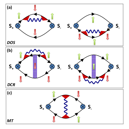
Figure 2: (Color online) The diagrams for spin susceptibility. The solid lines correspond to free electron Green’s functions, bold wavy lines to the fluctuation propagator, dashed triangles and rectangles account for electrons scatterings on impurities. The two diagrams (a) represent the density of states (DOS) correction, the diagrams (b) represent the renormalization of the diffusion coefficient (DCR), while the diagram (c) corresponds to the Maki-Thompson (MT) process.

Let us return to Fig. 2. The two diagrams (a) represent the effect of fluctuations on the single-particle self-energy, leading to a decrease in corresponding DOS at the Fermi level. Consequently, in accordance with the Korringa law, one can expect them to reduce the relaxation rate $W$ with respect to its normal value, opening some kind of fluctuation spin-gap upon approach of the transition line $H_{\mathrm{c2}}(T)$ from the normal phase.

Diagrams (b) with the four-leg Cooperon impurity blocks account for the corrections to the NMR relaxation rate due to the electron diffusion coefficient renormalization (DCR) by superconducting fluctuations. The analogous contribution turns out to be the dominant one in the region of quantum fluctuations in the case of fluctuation conductivityGlatz et al. (2011b). However, in the case under consideration, the additional integration over the external momentum with respect to the case of conductivity makes their contribution proportional to the square of the small Ginzburg-Levanyuk numberLarkin and Varlamov (2005)

$$\rm{Gi}_{\rm{2D}}=\frac{7\zeta(3)}{32\pi^{3}N(0)T_{\mathrm{c0}}\xi^{2}}\,,$$

which strongly suppresses the entire DCR contributionRanderia and Varlamov (1994).

Finally, the diagram in Fig. 2(c) is nothing else but the diagrammatic representation of the MT process shown in Fig. 1, where the region of attractive interaction (in grey) interrupted periodically by impurity scattering events (circles) is replaced by the fluctuation propagator (wavy line). This MT type diagram for $\chi_{\pm}$ in this graphic form appears to be identical to the one for conductivity. Nevertheless, the process shown in Fig. 1(c) shows us the important difference in the topology of the former and latter that arises from the spin structure. The MT diagram in Fig. 2(c) is a non-planar graph with a single fermion loop. In contrast, the MT graph for conductivity is planar and has two fermion loops. The number of loops, according to the rules of the diagrammatic techniqueAbrikosov et al. (1965), determines the sign of the contribution. In the case of spin susceptibility, which is under consideration, the topological sign of the MT diagram turns out to be opposite to that one for conductivity.

The presence of the $\hat{S}_{\pm}(\mathbf{k},\tau)$ operators, taking over the role of external vertices, changes not only the formal sign of the MT diagram. The fact that two fermion lines attached to such vertex must have the opposite spin labels (up and down) eliminates the Aslamazov-Larkin diagram from our present consideration: one simply cannot consistently assign a spin label to its central fermion lines for spin–singlet pairingManiv and Alexander (1977).

III DOS contribution

Let us start with the calculation of the DOS contribution determined by the two diagrams in Fig. 2(a). The corresponding expression for the dynamic spin susceptibility integrated over all momenta is

$$\int\left(d\mathbf{k}\right)\chi_{+-}^{\rm{DOS}}(\mathbf{k},\omega_{\nu})=\frac{h}{\pi\xi^{2}}\sum_{m}T\sum_{\Omega_{k}}L_{m}\left(\Omega_{k}\right)$$

$$\cdot T\sum_{\varepsilon_{n}}\lambda_{m}^{2}\left(\varepsilon_{n},\!\Omega_{k-n}\!\right)g\left(\varepsilon_{n+\nu}\!\right)J^{\rm{DOS}}\!\left(\varepsilon_{n},\Omega_{k-n}\right)\,,$$ (7)

where the first summation is performed over Landau levels and

$$g\left(\varepsilon_{n+\nu}\right)=\int\left(d\mathbf{k}\right)G\left(\mathbf{k},\varepsilon_{n+\nu}\right)=-i\pi N(0)\operatorname{sgn}\left(\varepsilon_{n+\nu}\right)\,,$$ (8)

$$J^{\rm{DOS}}\left(\varepsilon_{n},\Omega_{k-n}\right) =\int\left(d\mathbf{p}\right)~{}G^{2}\left(\mathbf{p},\varepsilon_{n}\right)G\left(\mathbf{p},\Omega_{k-n}\right)$$

$$=2\pi iN(0)\frac{\Theta\left(-\varepsilon_{n}\Omega_{k-n}\right)\operatorname{sgn}\left(\varepsilon_{n}\right)}{\left(i\widetilde{\varepsilon}_{n}-i\widetilde{\Omega}_{k-n}\right)^{2}}\,.$$ (9)

In the approximation of a dirty metal (${T\tau\ll 1})$,

$$\int\left(d\mathbf{k}\right)\, \chi_{+-}^{\rm{DOS}}(\mathbf{k},\omega_{\nu})=\frac{2\pi N^{2}(0)T^{2}h}{\xi^{2}}$$

$$\cdot\sum_{m}\sum_{\Omega_{k}}L_{m}\left(\Omega_{k}\right)\Xi_{m}\left(\Omega_{k},\omega_{\nu}\right)\,$$

with

$$\Xi_{m}\left(\Omega_{k},\omega_{\nu}\right)=\sum_{\varepsilon_{n}}\frac{\Theta\left(-\varepsilon_{n}\Omega_{k-n}\right)\operatorname{sgn}\left(\varepsilon_{n}\right)\operatorname{sgn}\left(\varepsilon_{n+\nu}\right)}{\left(\left|\varepsilon_{n}-\Omega_{k-n}\right|+\alpha_{m}\right)^{2}}\,,$$ (11)

where we have defined ${\alpha_{m}\equiv\omega_{c}\left(m+1/2\right)}$. For the Heaviside theta function we assume ${\Theta(0)=1}$. Now one can perform the summation over fermionic frequencies by splitting its domain into three intervals: ${(-\infty,-\nu-1]},{[-\nu,-1]},\text{ and }{[0,\infty)}$. The part of Eq. (III) depending on the external frequency $\omega_{\nu},$ which determines the imaginary part of the susceptibility $\mbox{Im}\chi_{+-}^{R}(\mathbf{k},-i\omega)$ in Eq. (2), is

$$\Xi_{m}^{\left(\omega\right)}\left(\Omega_{k},\omega_{\nu}\right)=-2\sum_{n=0}^{\nu-1}\frac{\Theta\left(\varepsilon_{n}+\Omega_{k}\right)}{\left(2\varepsilon_{n}+\Omega_{k}+\alpha_{m}\right)^{2}}\,.$$ (12)

The summation over fermionic frequencies again can be performed by splitting the domain of further summation over the bosonic frequencies into three: $k\in{[0,\infty)},\,k\in{[-\nu,-1]}$, and $k\in{(-\infty,-\nu-1]}$. Summation over the last interval results in zero and Eq. (12) is presented as the sum of regular and anomalous parts:

$$\Xi_{m}^{\left(\omega\right)}\left(\Omega_{k},\omega_{\nu}\right)=\Xi_{m}^{\left(\mathrm{reg}\right)}\left(\Omega_{k},\omega_{\nu}\right)+\Xi_{m}^{\left(\mathrm{an}\right)}\left(\Omega_{k},\omega_{\nu}\right)\,,$$ (13)

where

$$\Xi_{m}^{\left(\rm{reg}\right)}\left(\Omega_{k},\omega_{\nu}\right)=\frac{\Theta\left(\Omega_{k}\right)}{8\pi^{2}T^{2}}\left[\psi^{\prime}\left(\frac{1}{2}+\frac{\omega_{\nu}}{2\pi T}+\frac{\Omega_{k}+\alpha_{m}}{4\pi T}\right)-\psi^{\prime}\left(\frac{1}{2}+\frac{\Omega_{k}+\alpha_{m}}{4\pi T}\right)\right]$$ (14)

and

$$\Xi_{m}^{\left(\rm{an}\right)}\left(\Omega_{k},\omega_{\nu}\right)=\frac{\Theta\left(-\Omega_{k}\right)\Theta\left(\Omega_{k}+\omega_{\nu}\right)}{8\pi^{2}T^{2}}\left[\psi^{\prime}\left(\frac{1}{2}+\frac{\omega_{\nu}}{2\pi T}+\frac{\Omega_{k}+\alpha_{m}}{4\pi T}\right)-\psi^{\prime}\left(\frac{1}{2}+\frac{-\Omega_{k}+\alpha_{m}}{4\pi T}\right)\right]\,.$$ (15)

The regular part (14) is an analytic function of the external frequency $\omega_{\nu}$ and can be easily continued to the upper half-plane of the complex frequencies by substitution ${\omega_{\nu}\rightarrow-i\omega}$. As a result, by putting together Eqs. (2),(III), (11), and (14), one finds [the identity (6) was used to finalize $\Xi_{m}^{\left(\mathrm{reg}\right)}\left(\Omega_{k}\right)$]:

$$W^{\rm{DOS}\left(\mathrm{reg}\right)}(t,h)=\frac{AN(0)}{8\pi^{2}\xi^{2}}h\sum_{m=0}^{M}\sum_{k=0}^{\infty}\frac{4\mathcal{E}_{m}^{\prime\prime}\left(t,h,\left|k\right|\right)}{\mathcal{E}_{m}\left(t,h,\left|k\right|\right)}\,,$$ (16)

with $M=\left(tT_{\mathrm{c0}}\tau\right)^{-1}$ as the cut-off parameter.

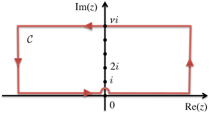
Figure 3: (Color online) Closed integration contour $\mathcal{C}$ in the plane of complex frequencies.

Now, let us proceed to the analysis of the anomalous DOS contribution to the relaxation rate determined by Eqs. (2), (III), (11), and (15). Here, the upper limit of summation over bosonic frequencies contains the external frequency and one should be cautious with the analytic continuation to the upper half-plane of complex frequencies. One can write

$$\int\left(d\mathbf{k}\right)\chi_{+-}^{\rm{DOS}\left(\mathrm{an}\right)}(\mathbf{k},\omega_{\nu})=-\frac{N(0)h}{2\pi\xi^{2}}\sum_{m}\theta_{m}\left(\omega_{\nu}\right)\,,$$ (17)

where

$$\theta_{m}\left(\omega_{\nu}\right)=\sum_{l=1}^{\nu-1}f_{m}(l,\omega_{\nu})$$ (18)

and

$$f_{m}(l,\omega_{\nu})=\frac{\left[\mathcal{E}_{m}^{\prime}\left(2\nu-l\right)-\mathcal{E}_{m}^{\prime}\left(l\right)\right]}{\mathcal{E}_{m}\left(l\right)}\,.$$ (19)

Note that the summation limit in Eq. (18) can be extended from ${(\nu-1)}$ to $\nu$, since ${f_{m}(l=\nu,\omega_{\nu})=0}$.

The analytic continuation of Eq. (18) to the upper half-plane of complex frequencies was performed in Ref. [Aslamasov and Varlamov, 1980] (see also Eq. (8.84) in Ref. [Larkin and Varlamov, 2005]). By means of the Eliashberg transformation Eliashberg (1961), the corresponding sum can be presented as an integral over a counterclockwise closed contour $\mathcal{C}$ consisting of two horizontal lines, two vertical lines, and a semicircle in the upper complex plane around the pole ${z=0}$ (see Fig. 3):

$$\theta_{m}\left(\omega_{\nu}\right)\!=\!\frac{1}{2i}\oint\limits_{\mathcal{C}}\coth\left(\pi z\right)f_{m}(-iz,\omega_{\nu})dz\,.$$ (20)

The integrals over the vertical line segments are zero and the integral over the semi-circle reduces to minus half of the residue of the integrand at ${z=0}$. By inverting the direction of integration along the line ${\mbox{Im}\,z=\nu}$ and shifting the integration variable as ${z-i\omega_{\nu}/2\pi T\rightarrow z}$ in the corresponding integral, one finds:

$$\theta_{m}\left(\omega_{\nu}\right)=-\frac{f_{m}(0,\omega_{\nu})}{2}+\frac{1}{2i}\mathop{\,\,\vphantom{\intop}\!\!\!\mathchoice{\ooalign{$\displaystyle\intop$\cr$\displaystyle-$}}{\ooalign{$\textstyle\intop$\cr$\textstyle-$}}{\ooalign{$\scriptstyle\intop$\cr$\scriptstyle-$}}{\ooalign{$\scriptscriptstyle\intop$\cr$\scriptscriptstyle-$}}}\nolimits_{-\infty}^{\infty}\coth\left(\pi z\right)$$ (29)

$$\times\left[f_{m}(\!-iz,\omega_{\nu})\!-\!f_{m}(\!-iz\!+\!\omega_{\nu}/2\pi T,\omega_{\nu})\right]dz\,.$$ (30)

Eq. (30) is an analytic function of $\omega_{\nu}$ and one can perform its continuation by the standard substitution ${\omega_{\nu}\rightarrow-i\omega}$. By the change of variables ${z+\omega/2\pi T\rightarrow z}$ in the second integral and with the help of the identity

$$\coth(a)-\coth(b)=-\frac{\sinh(a-b)}{\sinh(a)\sinh(b)}\,,$$

one finally finds

$$\theta_{m}^{R}\left(-i\omega\right)=-\frac{f_{m}(0,-i\omega)}{2}$$ (31)

$$+i\frac{\sinh\left(\omega/2T\right)}{2}\int_{-\infty}^{\infty}\frac{f_{m}(-iz,-i\omega)dz\!}{\sinh\left(\pi z\right)\sinh\left(\pi z-\omega/2T\right)}\,.$$

Substitution of the explicit expression for function ${f_{m}(-iz,-i\omega)}$ from Eq. (19) into Eq. (31) results in

$$\int\left(d\mathbf{k}\right)\chi_{+-}^{\rm{DOS}\left(\mathrm{an}\right)}(\mathbf{k},\omega)=-\frac{N(0)h}{4\pi\xi^{2}}\sum_{m=0}^{M}\left\{-\frac{\mathcal{E}_{m}^{\prime}\left(-\frac{i\omega}{\pi T}\right)-\mathcal{E}_{m}^{\prime}(0)}{\mathcal{E}_{m}(0)}\right.\left.+i\sinh\left(\frac{\omega}{2T}\right)\mathop{\,\,\vphantom{\intop}\!\!\!\mathchoice{\ooalign{$\displaystyle\intop$\cr$\displaystyle-$}}{\ooalign{$\textstyle\intop$\cr$\textstyle-$}}{\ooalign{$\scriptstyle\intop$\cr$\scriptstyle-$}}{\ooalign{$\scriptscriptstyle\intop$\cr$\scriptscriptstyle-$}}}\nolimits\limits_{-\infty}^{\infty}\frac{\left[\mathcal{E}_{m}^{\prime}\left(-iz\!-\!\frac{i\omega}{\pi T}\right)\!-\!\mathcal{E}_{m}^{\prime}(-iz)\right]dz\!}{\sinh(\pi z)\sinh\left(\pi z-\omega/2T\right)\mathcal{E}_{m}(-iz)}\right\}\,.$$ (40)

By sending the external frequency to zero, one finds the anomalous DOS contribution to the NMR relaxation rate:

$$W^{\rm{DOS}(\rm{an})}(t,h) = \frac{AN(0)}{8\pi^{2}\xi^{2}}h\sum_{m=0}^{M}\left\{\frac{2\mathcal{E}_{m}^{\prime\prime}(0)}{\mathcal{E}_{m}(0)}+2\pi\int_{-\infty}^{\infty}\frac{\mbox{Im}\,\mathcal{E}_{m}^{\prime}(iz)\,\mbox{Im}\,\mathcal{E}_{m}(iz)\,dz}{\sinh^{2}(\pi z)\left[\mbox{Re}^{2}\mathcal{E}_{m}(iz)+\mbox{Im}^{2}\mathcal{E}_{m}(iz)\right]}\right\}$$ (41)

Let us note that along the line $H_{\mathrm{c2}}(T),$ where the Eq. (5) can be simplified as

$$\mathcal{E}_{m}\left(t,h,iz\right)=\frac{h-h_{\mathrm{c2}}(t)}{h_{\mathrm{c2}}(t)}+\frac{i\pi^{2}zt}{4h_{\mathrm{c2}}(t)}\,,$$

the second term in Eq. (41) exactly cancels the first one and in this region only the regular part of the DOS diagrams contributes to the NMR relaxation rate. This fact justifies the approximation of static fluctuations (account for the term with $\Omega_{k}=0$ only) assumed in the previous worksManiv and Alexander (1977); Kuboki and Fukuyama (1989); Heym (1992); Randeria and Varlamov (1994); Eschrig et al. (1999); Mosconi et al. (2000) in their consideration performed close to $T_{\mathrm{c0}}.$

IV Maki-Thompson contribution

The mentioned above MT contribution to the process of NMR relaxation is described by the diagram in Fig. 2(c). The corresponding expression for the dynamic spin susceptibility integrated over all momenta is

$$\int\left(d\mathbf{k}\right)\chi_{+-}^{\rm{MT}}=\frac{hT^{2}}{2\pi\xi^{2}}\sum_{m}\sum_{\Omega_{k}}L_{m}\left(\Omega_{k}\right)\sum_{n}\lambda_{m}\left(\varepsilon_{n},\Omega_{k-n}\right)$$

$$\cdot\lambda_{m}\!\left(\varepsilon_{n+\nu},\Omega_{k-n-\nu}\right)\!I_{2g}\!\left(\varepsilon_{n},\Omega_{k-n}\right)\!I_{2g}\!\left(\varepsilon_{n+\nu},\Omega_{k-n-\nu}\right)$$ (42)

Restricting ourselves by the assumed above case of the dirty superconductor, one can write an explicit expression for the integral of the product of two Green’s functions:

$$I_{2g}\!=\!\!\int\!\!\left(d\mathbf{p}\right)\!G\!\left(\mathbf{p},\varepsilon_{n}\right)\!G\!\left(\mathbf{-p},\Omega_{k-n}\right)\!=\!2\pi N(0)\tau\Theta\!\left(-\varepsilon_{n}\Omega_{k-n}\right)$$

and express Eq. (42) in the standard form

$$\int\!\left(d\mathbf{k}\right)\chi_{+-}^{\rm{MT}}=\frac{2\pi N^{2}(0)T^{2}h}{\xi^{2}}\sum_{m}\sum_{\Omega_{k}}L_{m}\!\left(\Omega_{k}\right)\Upsilon_{m}\!\left(\Omega_{k},\omega_{\nu}\right)\,.$$

The summation over fermionic frequencies in the expression

$$\Upsilon_{m} = \sum_{n}\frac{\Theta\left[\varepsilon_{n}\left(\varepsilon_{n}-\Omega_{k}\right)\right]\Theta\left[\varepsilon_{n+\nu}\left(\varepsilon_{n+\nu}-\Omega_{k}\right)\right]}{\left(\left|2\varepsilon_{n}-\Omega_{k}\right|+\alpha_{m}\right)\left(\left|2\varepsilon_{n+\nu}-\Omega_{k}\right|+\alpha_{m}\right)}$$

$$= \Upsilon_{m}^{\left(\rm{reg1}\right)}\left(\Omega_{k},\omega_{\nu}\right)+\Upsilon_{m}^{\left(\rm{reg2}+\rm{an}\right)}\left(\Omega_{k},\omega_{\nu}\right)$$

is performed in complete analogy with the previous section, and one finds as a result:

$$\Upsilon_{m}^{\left(\rm{reg1}\right)}\left(\Omega_{k},\omega_{\nu}\right) = \frac{1}{4\pi T}\frac{1}{\omega_{\nu}}\left[\psi\left(\frac{1}{2}+\frac{2\omega_{\nu}+\left|\Omega_{k}\right|+\alpha_{m}}{4\pi T}\right)\right.$$

$$\left.-\psi\left(\frac{1}{2}+\frac{\left|\Omega_{k}\right|+\alpha_{m}}{4\pi T}\right)\right]\,$$

and

$$\Upsilon_{m}^{\left(\rm{reg2}+\rm{an}\right)}\left(\Omega_{k},\omega_{\nu}\right)=\frac{\Theta\left(\omega_{\nu-1}-|\Omega_{k}|\right)}{4\pi T\left(\omega_{\nu}+\alpha_{m}\right)}$$

$$\cdot\left[\psi\left(\frac{1}{2}+\frac{2\omega_{\nu}-|\Omega_{k}|+\alpha_{m}}{4\pi T}\right)-\psi\left(\frac{1}{2}+\frac{|\Omega_{k}|+\alpha_{m}}{4\pi T}\right)\right]\,.$$

Analitic continuation of $\Upsilon_{m}^{\left(\rm{reg1}\right)}\left(\Omega_{k},\omega_{\nu}\right)$ is trivial, while that one of $\Upsilon_{m}^{\left(\rm{reg2}+\rm{an}\right)}$ is performed by means of the Eliashberg transformation (20). Finally, one obtains

$$W^{\rm{MT}}(t,h) = \frac{AN(0)}{16\pi^{2}\xi^{2}}\,h\sum_{m=0}^{M}\left[\sum_{k=-\infty}^{\infty}\frac{4\mathcal{E}_{m}^{\prime\prime}\left(t,h,\left|k\right|\right)}{\mathcal{E}_{m}\left(t,h,\left|k\right|\right)}\right.$$

$$\left.+\frac{\pi^{3}}{\gamma_{\varphi}+\frac{2h}{t}(m+1/2)}\int\limits_{-\infty}^{\infty}\frac{dz}{\sinh^{2}(\pi z)}\frac{\mbox{Im}^{2}\mathcal{E}_{m}(t,h,iz)}{\mbox{Re}^{2}\mathcal{E}_{m}(t,h,iz)+\mbox{Im}^{2}\mathcal{E}_{m}(t,h,iz)}\right],$$

with ${\gamma_{\phi}=\pi/(8T_{\mathrm{c0}}\tau_{\phi})}$ and $\tau_{\phi}$ as the phase-breaking time.

V Main result

Collecting DOS and MT contributions in one expression and normalizing it to the normal metal Korringa relaxation rate, one can write the expression for $W^{\rm{fl}}$ valid in the whole phase diagram (with the restrictions discussed above):

$$\frac{W^{\rm{fl}}(t,h)}{W_{0}} = \frac{\rm{Gi}_{\rm{2D}}}{7\zeta(3)}\left(\frac{h}{t}\right)\sum_{m=0}^{M}\left[\sum_{k=-\infty}^{\infty}\frac{8\mathcal{E}_{m}^{\prime\prime}(t,h,\left|k\right|)}{\mathcal{E}_{m}(t,h,\left|k\right|)}\right.+4\pi\int_{-\infty}^{\infty}\frac{dz}{\sinh^{2}(\pi z)}\frac{\mbox{Im}\,\mathcal{E}_{m}^{\prime}(t,h,iz)\,\mbox{Im}\,\mathcal{E}_{m}(t,h,iz)}{\mbox{Re}^{2}\mathcal{E}_{m}(t,h,iz)+\mbox{Im}^{2}\mathcal{E}_{m}(t,h,iz)}$$ (43)

$$\left.+\frac{\pi^{3}}{\gamma_{\phi}+\frac{2h}{t}(m+1/2)}\int\limits_{-\infty}^{\infty}\frac{dz}{\sinh^{2}(\pi z)}\frac{\mbox{Im}^{2}\mathcal{E}_{m}(t,h,iz)}{\mbox{Re}^{2}\mathcal{E}_{m}(t,h,iz)+\mbox{Im}^{2}\mathcal{E}_{m}(t,h,iz)}\right]\,.$$

One can analyze it in different limiting cases.  Close to $T_{\mathrm{c0}}$ and for magnetic fields not too high (${h\ll 1}$) but arbitrary with respect to reduced temperature ${\epsilon=\left(T-T_{\mathrm{c0}}\right)/T_{\mathrm{c0}}\ll 1}$ and phase-breaking rate ${\gamma_{\phi}\ll 1}$ one can perform the integrations and summations in Eq. (43) and get

$$\frac{W^{\rm{fl}}(\epsilon,h\ll 1)}{W_{0}}=-3\rm{Gi}_{\rm{2D}}\left\{\left[\ln\frac{1}{h}-\psi\left(\frac{\epsilon}{2h}+\frac{1}{2}\right)\right]-\frac{\pi^{4}}{168\zeta(3)}\frac{1}{\epsilon-\gamma_{\phi}}\left[\psi\left(\frac{\epsilon}{2h}+\frac{1}{2}\right)-\psi\left(\frac{\gamma_{\phi}}{2h}+\frac{1}{2}\right)\right]\right\}.$$ (44)

In the limit of weak fields ${h\ll\min\{\epsilon,\gamma_{\phi}\}}$

$$\frac{W^{\rm{fl}}}{W_{0}} = \,3\rm{Gi}_{\rm{2D}}\left[\frac{\pi^{4}}{168\zeta(3)}\frac{1}{\epsilon-\gamma_{\phi}}\ln\frac{\epsilon}{\gamma_{\phi}}-\ln\frac{1}{\epsilon}\right]$$ (45)

$$-\rm{Gi}_{\rm{2D}}\,\frac{h^{2}}{2\epsilon^{2}}\left[\frac{\pi^{4}}{168\zeta(3)}\frac{\gamma_{\phi}+\epsilon}{\gamma_{\phi}^{2}}-1\right].$$

The first line of Eq. (45) reproduces the results of Refs. [Maniv and Alexander, 1977; Kuboki and Fukuyama, 1989; Heym, 1992; Randeria and Varlamov, 1994], while the magnetic field dependence of $W^{\rm{fl}}$ for weak fields (second line of Eq. (45)) was firstly analytically found in Ref. [Mosconi et al., 2000]. One can see that the MT contribution dominates when the pair-breaking is weak. In this case superconducting fluctuations in weak fields increase the NMR relaxation; increase of the field reduces the latter. As the phase-breaking grows, the role of the first term in Eq. (45) weakens and the effect of fluctuations can change sign: the MT trajectories shorten and the negative contribution of superconducting fluctuations due to the suppression of the quasi-particle density of states becomes the dominant. Since ${\gamma_{\phi}\lesssim 1}$ the effect of magnetic field on $W^{\rm{fl}}$ is always negative.

In the opposite case ${1\gg h\gg\max\left\{\epsilon,\gamma_{\phi}\right\}}$ the MT contribution dominatesMosconi et al. (2000): intrinsic pair-breaking here is weak while the effect of magnetic field on the motion of Cooper pairs is not yet strong enough:

$$\frac{W^{\rm{fl}}}{W_{0}}\approx\,3\rm{Gi}_{\rm{2D}}\left[\frac{\pi^{6}}{672\zeta(3)}\frac{1}{h}-\ln\frac{1}{h}\right].$$

Concluding discussion of the closeness of $T_{\mathrm{c0}}$, one can write the explicit expression for $W^{\rm{fl}}$ along the line $H_{\mathrm{c2}}(T)$ in its beginning, where ${\epsilon+h\rightarrow 0}$:

$$\frac{W^{\rm{fl}}}{W_{0}}=\,3\rm{Gi}_{\rm{2D}}\left\{\frac{\pi^{4}}{168\zeta(3)}\frac{2h}{(\epsilon+h)(\gamma_{\phi}+h)}-\ln\frac{1}{h}\right\}.$$

Now let us turn to the main subject of our study: the domain of the phase diagram above the second critical field at relatively low temperatures. Our general formula (44) allows to obtain the explicit analytical expressions, for instance, along the line $H_{\mathrm{c2}}(T)$, where ${t\ll h_{\mathrm{c2}}(t)}$. Here the main contribution is due to the lowest Landau level of the FCP motion. Corresponding propagator (3) has the pole structure:

$$L_{0}^{R}(t,h,iz)=-\frac{1}{N(0)}\frac{1}{\widetilde{h}+\frac{i\pi^{2}zt}{4h_{\mathrm{c2}}(t)}}.$$

Performing summation over bosonic frequencies and integration in Eq. (43) one finds

$$\frac{W^{\rm{fl}}\!\left(t\ll h_{\mathrm{c2}}(t)\right)}{W_{0}}=-\frac{4\pi^{2}\rm{Gi}_{\rm{2D}}}{7\zeta(3)}\left\{\ln\frac{1}{\widetilde{h}}+\frac{2\widetilde{h}\gamma_{\phi}}{\pi^{2}}\left[\psi^{\prime}\left(\frac{4h_{\mathrm{c2}}(t)\widetilde{h}}{\pi^{2}t}\right)-\frac{\pi^{2}t}{4h_{\mathrm{c2}}(t)\widetilde{h}}-\frac{1}{2}\left(\frac{\pi^{2}t}{4h_{\mathrm{c2}}(t)\widetilde{h}}\right)^{2}\right]\right\}$$

At very low temperatures ${t\ll\widetilde{h}}$, ${\widetilde{h}\equiv\left[H-H_{\mathrm{c2}}(0)\right]/H_{\mathrm{c2}}(0)}$, and just above $H_{\mathrm{c2}}(0),$ the regime of quantum fluctuations is realized. They suppress the NMR relaxation due to decrease of the quasi-particle density of states.

$$\frac{W^{\rm{fl}}\!\left(t\!\ll\!\widetilde{h}\right)}{W_{0}}=-\frac{4\pi^{2}\rm{Gi}_{\rm{2D}}}{7\zeta(3)}\!\left[\ln\frac{1}{\widetilde{h}}\!+\!\frac{\pi^{4}t^{3}\gamma_{\phi}}{192h_{\mathrm{c2}}^{3}(t)\widetilde{h}^{2}}\right]\,.$$ (46)

At higher temperatures, ${\widetilde{h}\ll t\ll h_{\mathrm{c2}}(t)}$, superconducting fluctuations become of thermal nature, while the DOS suppression of the NMR relaxation remains dominant:

$$\frac{W^{\rm{fl}}\!\left(\widetilde{h}\!\ll\!t\!\ll\!h_{\mathrm{c2}}(t)\!\right)}{W_{0}}\!=\!-\frac{4\pi^{2}\rm{Gi}_{\rm{2D}}}{7\zeta(3)}\!\!\left[\ln\frac{1}{\widetilde{h}}\!+\!\frac{\pi^{2}t^{2}\gamma_{\phi}}{16h_{\mathrm{c2}}^{2}(t)\widetilde{h}}\right]\,.$$ (47)

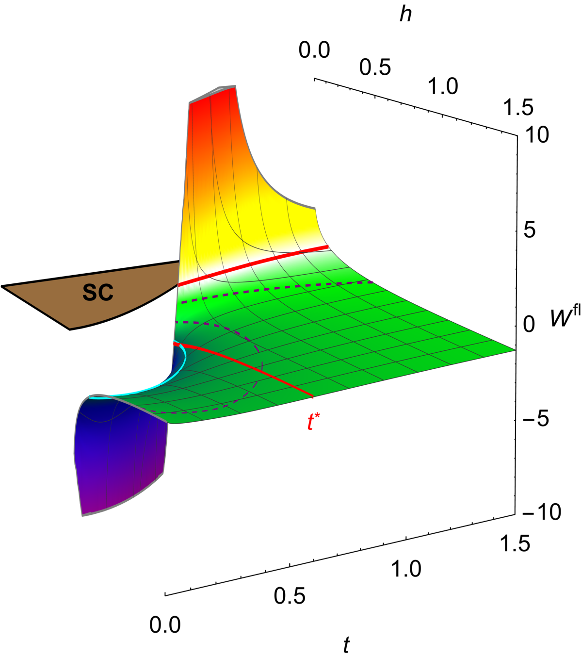
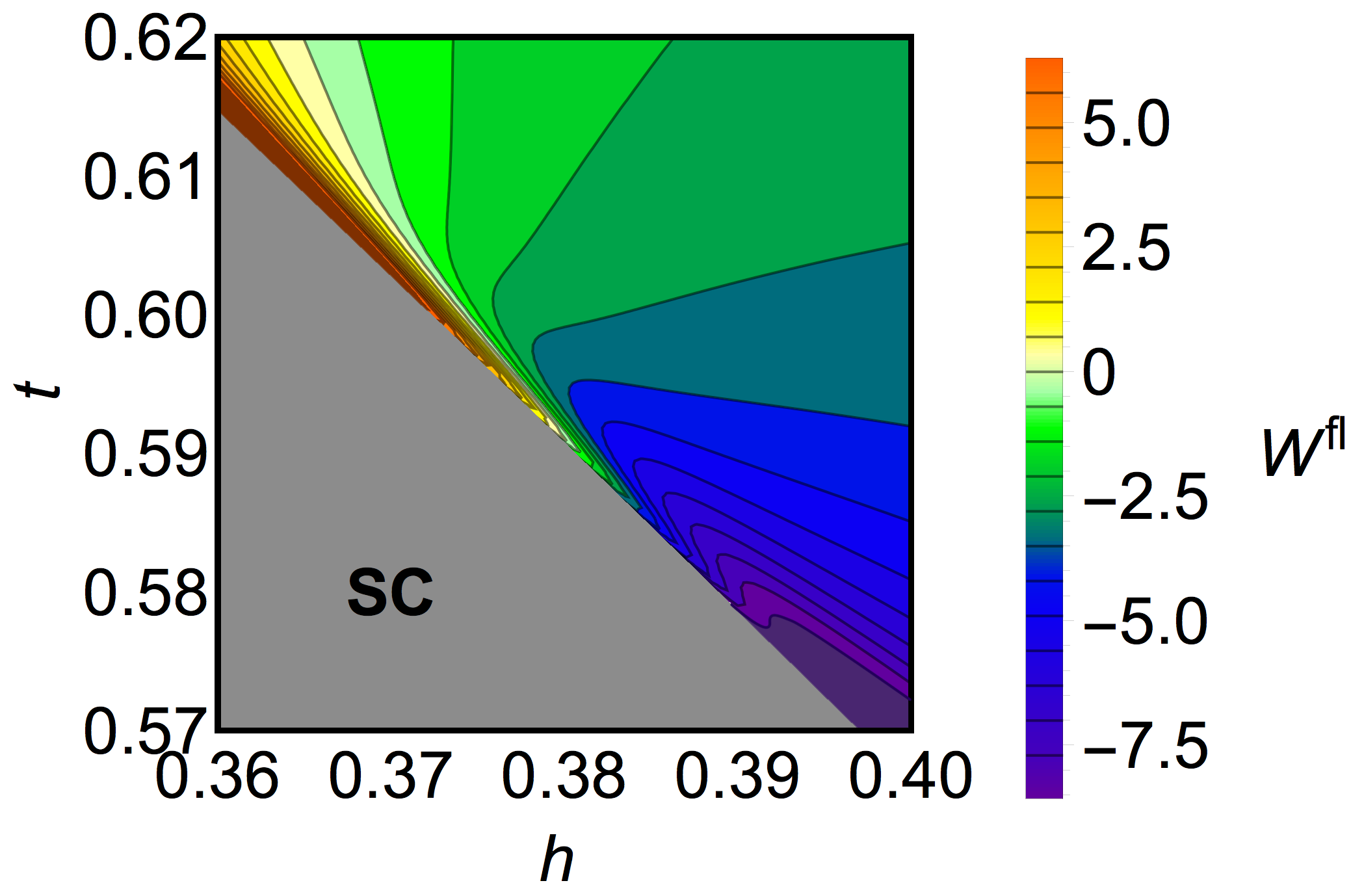
Figure 4: (Color online) Top: The temperature and magnetic field dependence of the relaxation rate $W^{\rm{fl}}$ in case of a very weak pair-breaking $\gamma_{\phi}=0.003$. The thick isoline (red) represents a zero relaxation rate, while the dashed isolines correspond to relaxation rate values of $-1$ and $-2$. The mesh-line $t^{*}$ (red) marks the critical temperature for $\gamma_{\phi}\to 0$, while the light (cyan) contour line indicates the value of $W^{\rm{fl}}$ at $h_{\rm{c2}}(t^{\ast})$ ($-3.04$) (see Fig. 6). Bottom: Contour plot of the region close to $h_{\mathrm{c2}}(t^{*})$.

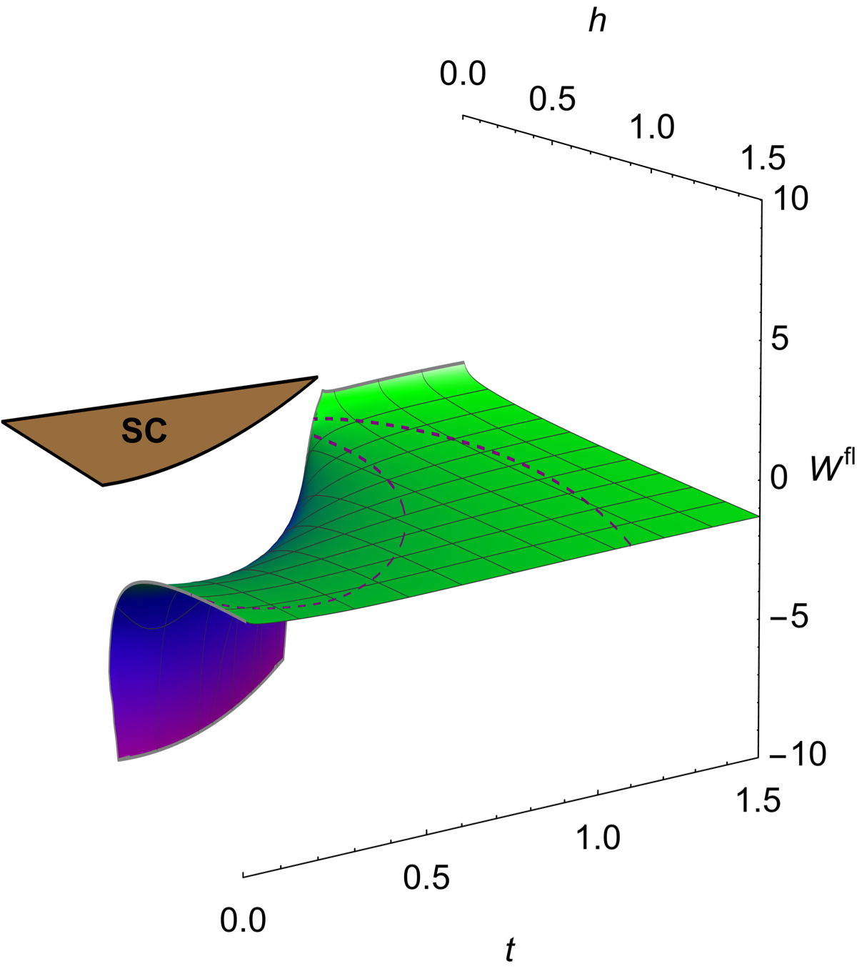
Figure 5: (Color online) The temperature and magnetic field dependence of the relaxation rate $W^{\rm{fl}}$ in case of a strong pair-breaking $\gamma_{\phi}=0.3$. The dashed isolines correspond to relaxation rate values of $-1.5$ and $-2$.

The results of numerical analysis of Eq. (43) for different pair-breaking rates are presented in Figs. 4–5. In the case of a small enough pair-breaking, there is a large domain of the phase diagram where superconducting fluctuations result in the increase of the NMR relaxation rate (see Fig. 4). Growth of the pair-breaking suppresses MT contribution and when ${\gamma_{\phi}\sim 1}$ the only effect of quasi-particle DOS suppression on $W^{\rm{fl}}$ dominates in the whole phase diagram (see Fig. 5). It is interesting that even in the absence of the pair-breaking (${\gamma_{\phi}\rightarrow 0}$) there exists a crossover temperature $T^{\ast}_{0}$ below which the MT relaxation process is suppressed by strong magnetic fields and the fluctuation correction $W^{\rm{fl}}$ cannot be positive. In the case of a two-dimensional superconductor $T_{0,\rm{2D}}^{\ast}\approx 0.6T_{\mathrm{c0}}.$ The temperature and field dependence of $W^{\rm{fl}}(T,H)$ near the point $\left\{T_{\rm{2D}}^{\ast},H_{\rm{c2}}\left(T_{\rm{2D}}^{\ast}\right)\right\}$ is very singular, see the close-up view of its vicinity in the bottom panel of Fig. 4.

Closer analysis of the crossover region, see Fig. 6, reveals that near $h_{\rm{c2}}(t^{\ast})$ the total correction curves calculated along the line $h_{\rm{c2}}(t)$ cross at a single point at temperature $t^{\ast}(\gamma_{\phi})$, i.e. the total correction to the NMR relaxation rate becomes independent of the field close to the point ${\{t^{\ast},h_{\rm{c2}}(t^{\ast})\}}$. This can also be seen on Fig. 4, where the isoline corresponding to the value ${W^{\rm{fl}}(t^{\ast},h_{\rm{c2}}(t^{\ast}))\approx-3.04}$ is seen to be parallel to the ${t=t^{\ast}}$ line in the immediate vicinity of the superconducting region.

Below the crossover temperature $t^{\ast}$, the total correction exhibits monotonic (increasing) field-dependence for fixed temperature ${t<t^{\ast}}$. For ${t\ll h_{\rm{c2}}(t)}$, both in the regime of quantum and thermal fluctuations, our numerical analysis is in full agreement with the asymptotic expressions (46) and (47), confirming the negative sign of the total correction. At the same time, Fig. 6 reveals a non-monotonic behavior at intermediate temperatures ${t\lesssim t^{\ast}}$ when going along the $h_{\rm{c2}}(t)$ line.

Above the crossover temperature, the field dependence of $W^{\rm{fl}}$ always shows a non-monotonic behavior as a result of the two competing contributions, as can be seen by from Fig. 4. The total correction is positive (for not-too-strong pair-breaking $\gamma_{\phi}$) close to the line $h_{\rm{c2}}(t)$; it then decreases rapidly reaching a minimum negative value at some intermediate distance from $h_{\rm{c2}}(t)$ before increasing up to zero when sufficiently far from the superconducting region.

Overall, our result for the total fluctuation correction $W^{\rm{fl}}$ is in qualitative agreement with that of Ref. Eschrig et al., 1999, where the temperature range between $0.75T_{\rm{c0}}$ and $1.5T_{\rm{c0}}$ was analyzed to compare with experimental data. The authors correctly point out the strong dependence of $W^{\rm{fl}}$ on the pair-breaking parameter $\gamma_{\phi}$. Our analysis based on Eq. (43) in the entire temperature range along $H_{\rm{c2}}(T)$ enables us to identify the temperature $T^{\ast}(\gamma_{\phi})$ at which the DOS and MT relaxation mechanisms fully compensate each other, such that the fluctuation correction ${W^{\rm{fl}}}$ completely vanishes (in the leading order of perturbation theory). The dependence of this temperature on the pair-breaking parameter $\gamma_{\phi}$ is presented in Fig. 6c). The asymptotic crossover temperature $T^{\ast}_{0}$ is then defined as $T^{\ast}(0)$, i.e. the temperature below which the negative DOS contribution always dominates, regardless of the values of $\gamma_{\phi}$ and $h$. The physical picture behind this observation is explained in more detail in Section VII.

VI Quasi-two-dimensional superconductor

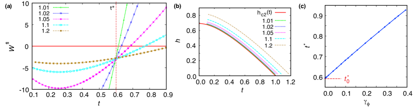
Figure 6: (Color online) Total correction (a) in the 2D case for $\gamma_{\phi}=0.003$ calculated parallel to, but at different distances from the line $h_{\mathrm{c2}}(t)$ in the fluctuation regime. Different colors correspond to different separations defined by the scaling parameter $a$ from $h_{\mathrm{c2}}(t)$ given in the legend, see the (b) panel. (c) $t^{\ast}(\gamma_{\phi})$ shows a linear dependence for all experimentally relevant values of $\gamma_{\phi}$. For fixed temperatures below $t^{\ast}$ the relaxation rate $W^{\rm fl}$ is monotonically increasing with field, while for larger temperatures the relaxation rate is non-monotonic and grows strongly when approaching $h_{c2}$ from above. The asymptotic value is $t^{\ast}_{0}=t^{\ast}(\gamma_{\phi}=0)=0.59$.

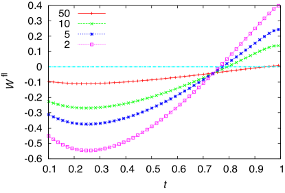
Figure 7: (Color online) Quasi-2D result for different $r$ values very close to $h_{\mathrm{c2}}(t)$ with $a=1.01$ (see Fig. 6) for $\gamma_{\phi}=0.003$.

The effect of three-dimensionality of the spectrum can be easily accounted for by the direct generalization of the Eq. (43). Indeed, the properties of a quasi-two dimensional superconductor can be described well in the framework of the phenomenological Lawrence-Doniach (LD) modelLD7 (1971), which provides a Ginzburg-Landau functional for a layered superconductor. In the case under consideration, when the magnetic field is applied perpendicular to the layers, it takes the form:

$$\mathcal{F}^{(\rm{LD})}\!\left[\Psi\right] = {\sum_{l}}\!\int\!d^{2}r\!\left[\!\alpha T_{\mathrm{c0}}\epsilon\left|\Psi_{l}\right|^{2}\!+\!\frac{b}{2}\left|\Psi_{l}\right|^{4}\right.$$

$$\left.+\frac{1}{4m}\left|\left(\mathbf{\nabla}_{\parallel}\!-\!2ie\mathbf{A}_{\parallel}\right)|\Psi_{l}\right|^{2}\!+\!\mathcal{J}\left|\Psi_{l+1}-\Psi_{l}\right|^{2}\right].$$

Here $\Psi_{l}$ is the order parameter of the $l$-th superconducting layer and the phenomenological constant $\mathcal{J}$ is proportional to the energy of the Josephson coupling between adjacent planes. The gauge with ${A_{z}=0}$ is chosen.

In the immediate vicinity of $T_{\mathrm{c}}$, the LD functional is reduced to the GL one with the effective mass ${M=\left(4\mathcal{J}s^{2}\right)^{-1}}$ along $z$-direction, where $s$ is the inter-layer spacing. One can relate the value of $\mathcal{J}$ to the coherence length along the $z$-direction, or, what is more convenient, with the degree of three-dimensionality of the system ${r=4\xi_{z}^{2}/s^{2}}$: ${\mathcal{J}=\alpha T_{\mathrm{c0}}r/2}$ (see Ref. [Larkin and Varlamov, 2005] pp. 26 and 220). Corresponding generalization can be done also in the microscopic approach: it is enough to enrich the propagator and Cooperons (or directly the final Eq. (43)) by the account of the transversal motion: ${\omega_{\mathrm{c}}\left(m+\frac{1}{2}\right)\rightarrow\omega_{\mathrm{c}}\left(m+\frac{1}{2}\right)+\frac{\mathcal{J}}{2}(1-\cos q_{z}s)}$ and perform the additional integration over the transversal momentum. In order to avoid the cumbersome expressions, let us show explicitly how it works only for the regular DOS contribution (16):

$$W^{\rm{DOS}(\rm{LD},\mathrm{reg})}(t,h)=\frac{AN(0)}{8\pi^{2}\xi^{2}}h\int_{-\pi/s}^{\pi/s}\frac{dq_{z}}{2\pi}\sum_{m=0}^{M}\sum_{k=0}^{\infty}\frac{\psi^{\prime\prime}\left[\frac{1+|k|}{2}+\frac{2h}{t}\frac{\left(2m+1\right)}{\pi^{2}}+\frac{4r}{\pi^{2}t}\sin^{2}\frac{q_{z}s}{2}\right]}{\ln t+\psi\left[\frac{1+|k|}{2}+\frac{2h}{t}\frac{\left(2m+1\right)}{\pi^{2}}+\frac{4r}{\pi^{2}t}\sin^{2}\frac{q_{z}s}{2}\right]-\psi\left(\frac{1}{2}\right)}.$$ (48)

One can see that the averaging in Eq. (48) over the transversal modes effectively reduces it to the same Eq. (16) with addition of some positive constant $\lambda r/t$ in the arguments of all polygamma functions. Hence, in order to satisfy the same conditions for ${T^{\ast}\left(r=0\right)}$ but at some temperature ${T^{\ast}\left(r>0\right)}$, one should have

$$\frac{h_{\mathrm{c2}}\left(t_{\rm{2D}}^{\ast}\right)}{t_{\rm{2D}}^{\ast}}=\frac{h_{\mathrm{c2}}\left(t_{r}^{\ast}\right)}{t_{r}^{\ast}}+\pi^{2}\lambda\frac{r}{t_{r}^{\ast}}.$$

This means that ${h_{\mathrm{c2}}\left(t_{\rm{2D}}^{\ast}\right)/t_{\rm{2D}}^{\ast}>h_{\mathrm{c2}}\left(t_{r}^{\ast}\right)/t_{r}^{\ast}}$, or, taking into account the monotonous increase of the second critical field with the decrease of temperature, one makes sure that ${t_{r}^{\ast}>t_{\rm{2D}}^{\ast}}$, i.e. the temperature $T^{\ast}$ should grow with the increase of $r.$ This qualitative speculation is confirmed by the numerical study of correspondingly generalized Eq. (43) (see Fig. 7), where the asymptotic crossover temperature is increased to ${t^{\ast}_{0,\rm{3D}}\approx 0.75}$.

VII Discussion

Here we discuss the physical aspect of the results obtained and consequences for the general understanding of the fluctuation picture. As already explained above, it is the MT process of the self-electron pairing at the self-intersecting trajectories that is responsible for the growth of $W(T,H).$ Its contribution to the NMR relaxation rate is proportional to the superconducting interaction strength $g\left(T,H\right)$ and to the total probability for the formation of such trajectories (see Ref. [Larkin and Varlamov, 2005]):

$$W_{\rm{2D}}^{\rm{MT}}(T,H)\sim g(T,H)\int_{\xi_{\rm{FCP}}\left(T,H\right)/v_{F}}^{\min\{\ell_{\phi},L_{H}\}/v_{F}}\frac{\lambda_{F}v_{F}dt}{Dt}.$$

Here $L_{H}=\sqrt{c/2eH}$ is the FCP magnetic length, while ${\xi_{\rm{FCP}}(T,H)}$ is its effective size. Close to $T_{\mathrm{c0}}$ and in weak fields, where the long wave-length Ginzburg-Landau fluctuation picture takes place ${\xi_{\rm{FCP}}(T,H)=\xi_{\rm{GL}}=\xi_{\rm{xy}}/\sqrt{\epsilon}}$. In the opposite case of quantum fluctuations at zero temperature and in the vicinity of $H_{\mathrm{c2}}(0)$, the size of FCP clusters, including many pairs, is of the order of ${\xi_{\rm{xy}}/\sqrt{\widetilde{h}}}$, but the length corresponding to one of them is ${\xi_{\rm{FCP}}(0,H)\sim\xi_{\rm{xy}}}$ (see Refs. [Glatz et al., 2011a] and [Glatz et al., 2011b]). At some intermediate region of temperatures along the line $H_{\mathrm{c2}}(T)$ to low temperatures the increasing magnetic field “breaks” GL waves and the vortex description becomes more adequate. The obtained crossover temperature $T^{\ast}$ allows us to define where it happens: namely for ${\xi_{\rm{FCP}}\left[T^{\ast},H(T^{\ast})\right]\sim L_{H}=\sqrt{c/2eH(T^{\ast})}}$, where the MT mechanism of NMR relaxation becomes irrelevant when going to lower temperatures (see Figs. 4 and 6). The crossover temperature depends on the pair-breaking parameter $\gamma_{\phi}$ and becomes minimal in the limit ${\gamma_{\phi}\rightarrow 0}$ with a value ${t^{\ast}_{0}\approx 0.6}$ which can be clearly seen in Figs. 4 and 5.

Now let us return to discussion of the experiments of Ref. [Lascialfari and Rigamonti, shed; Lascialfari et al., 2005], which partially motivated this work. The authors observed a well pronounced peak of $W(T,H)$ versus magnetic field in the low temperature part ($t=0.12;0.25)$ when crossing the line $H_{\mathrm{c2}}(T)$ and attributed it to the possible manifestation of the quantum fluctuations. Unfortunately, our analysis of all fluctuation contributions definitely excludes this hypothesis: below ${t^{\ast}_{0}\approx 0.6}$ fluctuations can only open the spin gap in the NMR relaxation rate, but they cannot lead to its growth. The observed decay above $H_{\mathrm{c2}}(T)$ is therefore not related to quantum fluctuations.

VIII Acknowledgements

We express our deep gratitude to A. Rigamonti and A. Lasciafari for attracting our attention to their experiments and numerous elucidating discussions. A.V. was partially supported by the U.S. Department of Energy, Office of Science, Office of Advanced Scientific Computing Research and Materials Sciences and Engineering Division, Scientific Discovery through Advanced Computing (SciDAC) program.

Appendix A Numerical evaluation of the NMR relaxation rate

In order to utilize the complete expression for the NMR relaxation rate $W^{\rm{fl}}$ to analyze experimental data we need an efficient and accurate method to evaluate Eq. (43) numerically. Here we describe the method used throughout this work. The integral contributions ($z$-integrations) can be straight-forwardly evaluated using a suitable quadrature scheme. Here we use the Gauss-Legendre 5-point method, which also allows integration of integrable poles or principle values. Due to the presence of the $\sinh^{-2}(\pi z)$ term in the integrand we can restrict the support to $z\in[-5,5]$. Outside this interval the integrand is smaller than the numerical accuracy (of double precision floating point numbers). This sum over Landau-levels is calculated up to $M=(tT_{\mathrm{c0}}\tau)^{-1}$ explicitly.

In contrast, the summation over $k$ in the MT contribution to Eq. (43) is more involved and only slowly converging. For the numerical summation of the $k$-sum we separate the $k=0$ term and sum from $k=1$ to $k_{\max}$ (twice, due to symmetry) which is determined by the arguments of the $\mathcal{\psi}^{(n)}$ functions being equal to $\Omega=1000$. For $k\geq k_{\max}$ we transform the sum into an integral and use only the asymptotic expressions for the polygamma functions as the difference to the exact expression is again below the floating point accuracy. Then the integration variable is inverted and we have a finite integral for the remaining part of the sum.

Therefore we concentrate on

$$S^{\rm{MT}}_{m}\equiv\sum_{k=-\infty}^{\infty}\frac{\mathcal{E}_{m}^{\prime\prime}\left(t,h,\left|k\right|\right)}{\mathcal{E}_{m}\left(t,h,\left|k\right|\right)}$$

and write

$$S_{m}^{\rm{MT}} = \left[\sum_{k=0}^{k_{\max}-1}\left(2-\delta_{0,k}\right)+2\int_{k_{\max}}^{\infty}dk\right]\frac{\mathcal{E}_{m}^{\prime\prime}\left(t,h,\left|k\right|\right)}{\mathcal{E}_{m}\left(t,h,\left|k\right|\right)}$$

$$\equiv S_{m}^{\rm{MT}(s)}+S_{m}^{\rm{MT}(i)}$$

with

$$k_{\max}=\max\left\{2\Omega-\left\lfloor\frac{4h}{\pi^{2}t}\left(2m+1\right)\right\rfloor,1\right\}\,.$$

The sum part $S^{\rm{MT}(s)}_{m}$ is calculated straightforwardly, which leaves the calculation of the “rest-integral” $S^{\rm{MT}(i)}_{m}$:

$$S_{m}^{\rm{MT}(i)} = \frac{1}{2}\int\limits_{k_{\max}}^{\infty}\!\!dk\,\frac{\psi^{\prime\prime}\left(\frac{1+k}{2}+x_{m}\right)}{\ln t-\psi\left(\frac{1}{2}\right)+\psi\left(\frac{1+k}{2}+x_{m}\right)}$$

$$\circeq \!-\frac{1}{2}\!\int\limits_{k_{\max}}^{\infty}\!\!dk\,\frac{\left(\frac{1+k}{2}+x_{m}\right)^{-2}}{\ln t-\psi\left(\frac{1}{2}\right)-\ln(2)+\ln\left(1+k+2x_{m}\right)}$$

with $x_{m}\equiv\frac{2h}{t}\frac{\left(2m+1\right)}{\pi^{2}}$.

A convenient substitution is

$$\frac{1}{z}\!=\!\frac{8}{\pi^{2}}+\frac{(1+k)t}{h\left(m+1/2\right)}=\frac{8}{\pi^{2}x_{m}}\left[x_{m}+\frac{1+k}{2}\right]\,,$$

$$\frac{dz}{z^{2}}=-\frac{t}{h\left(m+1/2\right)}dk=-\frac{4}{\pi^{2}}\frac{dk}{x_{m}}\,,$$

$$z_{\max}=\frac{\pi^{2}}{4}\left(2+\frac{1+k_{\max}}{x_{m}}\right)^{-1}\,.$$

Therefore,

$$S_{m}^{\rm{MT}(i)}\! = \!\frac{\pi^{2}}{8}\int\limits_{z_{\max}}^{0}\frac{dz}{z^{2}}\!\frac{x_{m}\left(\frac{8z}{\pi^{2}x_{m}}\right)^{2}}{\ln\left(t\pi^{2}x_{m}/4\right)-\psi\left(\frac{1}{2}\right)-\ln(2)-\ln(z)}$$

$$= -\frac{8}{\pi^{2}x_{m}}\int\limits_{0}^{z_{\max}}dz\frac{1}{A_{m}-\ln z}$$

$$= -\frac{2t}{h\left(m+1/2\right)}\int\limits_{0}^{z_{\max}}dz\frac{1}{A_{m}-\ln z}$$

with $A_{m}\equiv\ln\left[h\left(m+1/2\right)\right]-\psi\left(\frac{1}{2}\right)-\ln(2)$.

This integral is integrable and calculated by the Gauss-Legendre 5-point method (with avoids the singular point at $z=0$) with only a few support points in the small interval $0$ to $z_{max}$ using $125$ support points.

Overall this yields a highly accurate numerical value of the $k$-sums.

In the quasi-two-dimensional case the additional finite $q$-integral is calculated by the Gauss-Legendre 5-point method using $25$ support points, which is sufficient to obtain high accuracy.