Comparing Hamiltonians of a spinning test particle for different tetrad fields

Abstract

This work is concerned with suitable choices of tetrad fields and coordinate systems for the Hamiltonian formalism of a spinning particle derived in [E. Barausse, E. Racine, and A. Buonanno, Phys. Rev. D 80, 104025 (2009)]. After demonstrating that with the originally proposed tetrad field the components of the total angular momentum are not preserved in the Schwarzschild limit, we analyze other hitherto proposed tetrad choices. Then, we introduce and thoroughly test two new tetrad fields in the horizon penetrating Kerr–Schild coordinates. Moreover, we show that for the Schwarzschild spacetime background the linearized in spin Hamiltonian corresponds to an integrable system, while for the Kerr spacetime we find chaos which suggests a nonintegrable system.

I Introduction

The motion of a spinning particle in the spacetime background of a black hole, particularly the Kerr spacetime, is of great astrophysical interest. Namely, it approximates the motion of a stellar compact object (e.g., a black hole) around a supermassive black hole. Such binary systems are expected to lie at the center of galaxies (see, e.g., AmaroSeoane14 and references therein) and to be good candidates for sources of gravitational radiation Riles13 .

Even though the equations describing the motion of a spinning particle in a curved spacetime have been provided several decades ago by Mathisson Mathisson37 and Papapetrou Papapetrou51 , many issues of this motion are still open. The problem lies in the fact that the Mathisson-Papapetrou (MP) equations are not a closed system of first order differential equations. Hence, a spin supplementary condition (SSC) is needed in order to close them. Several such SSCs have been proposed (see, e.g., Semerak99 ; Kyrian07 for a review), each of which introduces a different reference frame. Physically, the ambiguity in the choice of a SSC is related to the fact that a spinning body cannot be treated as a point particle but must have a finite size in order to be prevented from rotating at superluminal speed Moeller49 . In particular, each SSC corresponds to an observer who sees the reference worldline fixed by the SSC as the center of mass of the extended body. Previous studies have shown that the choice of the SSC depends on the question one wants to investigate Costa12 ; Corinaldesi51 ; Kyrian07 ; Semerak99 ; LSK1 ; Moeller49 ; Pirani56 ; Semerak15 .

Within the MP equations the motion of spinning test particles in the Schwarzschild or Kerr spacetime have been investigated in Hackmann14 ; Plyatsko12 ; Plyatsko13 , and several papers have been devoted to the investigation of the appearing chaotic motion Hartl03a ; Hartl03b ; Suzuki97 ; Verhaaren10 . Beyond the pole-dipole approximation, the quadrupole moment of the test particle has already been taken into account Steinhoff12 ; Bini14 .

The dynamics of spinning test particles has not only been worked out in Lagrangian formalisms (MP equations) Bailey75 , but in Hamiltonian formalisms Steinhoff11 ; Steinhoff08 ; Barausse09 ; Tauber88 ; Deriglazov15a ; Deriglazov15b as well. Hamiltonian dynamics has a long tradition in astronomy and a large number of problems there (e.g., perturbative problems or chaotic motion) are typically studied from a Hamiltonian perspective Contop02 . In general relativity the Hamiltonian formalisms have been applied, for example, in the framework of the canonical Arnowitt-Deser-Misner (ADM) formalism ADM and in the effective-one-body approach (EOB) Buonanno99 ; Damour00 ; Damour08 , which studies the dynamics of spinning bodies of compact objects using the Hamiltonian description of a one-body problem Blanchet06 . Due to the significance of a Hamiltonian approach the Hamiltonian description of spinning particles is important despite the fact that it mostly neglects terms quadratic in spin.

In our previous work LSK1 , we have compared the Tulczyjew (T) SSC Tulczyjew59 with the Newton-Wigner (NW) SSC NewtonWigner49 as supplements to the MP equations. In a second step, we compared the MP equations supplemented by the NW SSC to the corresponding Hamilton equations derived in Barausse09 based on the same NW SSC. In this work we focus on the latter, i.e., on a canonical Hamiltonian formalism which should be equivalent to the MP equations up to the linear order of the test particle spin.

In contrast to the T SSC, the NW SSC, which is used within the framework of the Hamiltonian formalism, does not provide a unique choice of reference frame. It rather defines an entire class of observers, each characterized by a different tetrad field. Thus, the Hamiltonian formalism proposed in Barausse09 depends on the choice of a reference basis given by such a tetrad field. Each choice of a tetrad field basically determines the form and the properties of the resulting Hamiltonian function. The fact that tetrads providing certain frames of reference are involved in a definition of the spin variable can also be seen as a consequence of the fact that in the Hamiltonian description the spin is a vector with prescribed canonical relations to coordinates and momenta. Still, one might conclude that the tetrad dependence of the Hamiltonian description of the spinning particle is against covariance principles of general relativity. Yet, when we numerically solve equations of motion we have to use some coordinates anyway. The involvement of tetrads simply means we use different coordinates for external and inner degrees of freedom of the spinning particle. As, e.g., Boyer-Lindquist coordinates are comfortable for solving equations of motion in Kerr geometry there may well be some other tetrad fields more suitable for the definition of the Hamiltonian spin.

We discuss the advantages and the drawbacks of Hamiltonian functions arising from tetrad fields already proposed in Barausse09 ; Barausse10 . Then, we introduce two new tetrad fields in Kerr–Schild coordinates which yield Hamiltonian functions with desirable properties using both analytical and numerical analysis. Namely in order to have a good choice of a tetrad field, the corresponding Hamiltonian should reflect the symmetries of the background spacetime, i.e., preserve the integrals of motion, and avoid any coordinate effects evoked by coordinate dependent tetrad basis vectors. For the above discussion, we focus on the Schwarzschild limit and show that the well behaving Hamiltonian functions based on our tetrads have as many integrals of motion as degrees of freedom. Thus, it is shown that in the Schwarzschild limit these Hamiltonians describe an integrable system. We view this as an important test, as in general, for different tetrad fields the description Barausse09 provides Hamiltonians non-equivalent beyond the given approximation. In any Hamiltonian system the integrals of motion play a crucial role, when the integrability issue is studied. If we have several possible descriptions of the same system in the given approximation, those respecting all background symmetries are the obvious choice. We use the case of spinning particle in Schwarzschild spacetime as such an exact problem with many integrals of motion to demonstrate shortcomings of certain coordinate-tetrad choices. Even though the considered approximations assume small spins, to clearly demonstrate (non-)integrability we also use large spin values in numerical tests.

As for the Kerr spacetime, it was shown in Rudiger that if the MP equations supplemented by the T SSC are linearized in the spin, an integral of motion associated with a Killing-Yano tensor appears. This led to the impression that, up to linear order in the spin, the motion of a spinning particle is integrable in general Hinderer13 . However, according to our numerical calculations, this seems not to be the case for the Hamiltonian function depending on the tetrad field choice introduced in Barausse10 .

This paper is organized as follows. In Sec. II we give a short overview of the Hamiltonian formalism introduced in Barausse09 . After that, in Sec. III, we present two different choices of coordinate systems, the Boyer-Lindquist and the Cartesian isotropic coordinates, for a tetrad corresponding to a ZAMO observer which is already given in Barausse09 ; Barausse10 . We analyze the properties of both with the help of analytical calculations and numerical integrations. Then we present our new tetrads in Kerr-Schild coordinates in Sec.  IV. Finally, in Sec.  V, we summarize our results. We add a description of our numerical tools in the Appendix.

We use geometric units, i.e., $(G=c=1)$, and the signature of the metric is (-,+,+,+). Greek letters denote the indices corresponding to spacetime (running from 0 to 3), while Latin letters denote indices corresponding only to space (running from 1 to 3).

II The Hamiltonian formalism

The Hamiltonian formalism in Barausse09 has been achieved by linearizing the MP equations of motion for the NW SSC. The MP equations describe the motion of a particle with mass $m^{2}=-p_{\mu}p^{\mu}$, satisfying the mass shell constraint, and spin $S^{\mu\nu}$ in a given spacetime background $g_{\mu\nu}$. Their reformulation in Dixon70 reads

$$\frac{D\leavevmode\nobreak\ p^{\mu}}{d\sigma}=-\frac{1}{2}\leavevmode\nobreak\ {R^{\mu}}_{\nu\kappa\lambda}v^{\nu}S^{\kappa\lambda}\leavevmode\nobreak\ \leavevmode\nobreak\ ,$$ (1)

$$\frac{D\leavevmode\nobreak\ S^{\mu\nu}}{d\sigma}=p^{\mu}\leavevmode\nobreak\ v^{\nu}-v^{\mu}\leavevmode\nobreak\ p^{\nu}\leavevmode\nobreak\ \leavevmode\nobreak\ ,$$ (2)

where $p^{\mu}$ is the four-momentum, $v^{\mu}=dx^{\mu}/d\sigma$ is the tangent vector to the worldline along which the particle moves, $\sigma$ is an evolution parameter along this worldline, and ${R^{\mu}}_{\nu\kappa\lambda}$ is the Riemann tensor. The NW SSC reads

$$S^{\mu\nu}\leavevmode\nobreak\ \omega_{\mu}=0\leavevmode\nobreak\ \leavevmode\nobreak\ ,$$ (3)

where $\omega_{\mu}$ is a sum of timelike vectors. This sum in Barausse09 has the form

$$\omega_{\nu}=p_{\nu}-m\leavevmode\nobreak\ \tilde{e}_{\nu}\,^{T}\leavevmode\nobreak\ \leavevmode\nobreak\ ,$$ (4)

where $\tilde{e}_{\nu}\,^{T}$ is a timelike future oriented vector (throughout the article we use T instead of 0), which together with three spacelike vectors $\tilde{e}^{\mu}\,_{I}$, denoted by capital latin indices, is part of a tetrad field $\tilde{e}^{\mu}\,_{\Delta}$.

This tetrad field has to satisfy two conditions: the first condition ensures the orthonormality of the tetrad given by

$$\tilde{e}^{\mu}\,_{\Gamma}\tilde{e}^{\nu}\,_{\Delta}\leavevmode\nobreak\ g_{\mu\nu}=\eta_{\Gamma\Delta}\leavevmode\nobreak\ \leavevmode\nobreak\ ,$$ (5)

where $\eta_{\Gamma\Delta}$ is the metric of the flat spacetime and $g_{\mu\nu}$ its analogon for the curved spacetime background. The capital indices are raised and lowered by the flat metric $\eta_{\Gamma\Delta}$, the small ones by $g_{\mu\nu}$. The second condition is implied by (5) and reads

$$\tilde{e}^{\mu}\,_{\Delta}\tilde{e}_{\nu}\,^{\Delta}=\delta_{\nu}^{\mu}\leavevmode\nobreak\ \leavevmode\nobreak\ ,$$ (6)

where $\delta_{\nu}^{\mu}$ is the Kronecker delta.

When a tensor is projected on the tetrad field, then it is denoted with capital indices. For example, $\omega_{\Delta}=\tilde{e}^{\nu}\,_{\Delta}\omega_{\nu}$ is the projection of the time-like vector (4) on the tetrad field, i.e.,

$$\omega_{T} = p_{\nu}\leavevmode\nobreak\ \tilde{e}^{\nu}\,_{T}-m\leavevmode\nobreak\ \leavevmode\nobreak\ ,$$

$$\omega_{J} = p_{\nu}\leavevmode\nobreak\ \tilde{e}^{\nu}\,_{J}\leavevmode\nobreak\ \leavevmode\nobreak\ .$$ (7)

Then, the spin tensor $S^{\mu\nu}$ projection reads

$$S^{IJ}=S^{\mu\nu}\leavevmode\nobreak\ \tilde{e}_{\mu}\,^{I}\leavevmode\nobreak\ \tilde{e}_{\nu}\,^{J}\leavevmode\nobreak\ \leavevmode\nobreak\ .$$ (8)

In Barausse09 , the authors do not work with this tensor but rather employ the spin three vector

$$S_{I}=\frac{1}{2}\epsilon_{IJL}\leavevmode\nobreak\ S^{JL}\leavevmode\nobreak\ \leavevmode\nobreak\ ,$$ (9)

where $\epsilon_{IJL}$ is the Levi-Civita symbol.

Now, the Hamiltonian function $H$ for a spinning particle

$$H=H_{NS}+H_{S}\leavevmode\nobreak\ \leavevmode\nobreak\ ,$$ (10)

splits in two parts. The first,

$$H_{NS}=\beta^{i}P_{i}+\alpha\leavevmode\nobreak\ \sqrt{m^{2}+\gamma^{ij}P_{i}P_{j}}\leavevmode\nobreak\ \leavevmode\nobreak\ ,$$ (11)

is the Hamiltonian for a nonspinning particle, where

$$\alpha = \frac{1}{\sqrt{-g^{00}}}\leavevmode\nobreak\ \leavevmode\nobreak\ ,$$ (12)

$$\beta^{i} = \frac{g^{0i}}{g^{00}}\leavevmode\nobreak\ \leavevmode\nobreak\ ,$$ (13)

$$\gamma^{ij} = g^{ij}-\frac{g^{0i}g^{0j}}{g^{00}}\leavevmode\nobreak\ \leavevmode\nobreak\ ,$$ (14)

and $P_{i}$ are the canonical momenta conjugate to $x^{i}$ of the Hamiltonian (10). They can be calculated from the momenta $p_{i}$ with the help of the relation

$$P_{i} = p_{i}+E_{i\Gamma\Delta}S^{\Gamma\Delta}\leavevmode\nobreak\ \leavevmode\nobreak\ ,$$ (15)

$$= p_{i}+\left(2E_{iTJ}\frac{\omega_{C}}{\omega_{T}}+E_{iJC}\right)\epsilon^{JCL}\leavevmode\nobreak\ S_{L}\leavevmode\nobreak\ \leavevmode\nobreak\ ,$$

where the spin connection

$$E_{\nu\Gamma\Delta}=-\frac{1}{2}\left(g_{\kappa\lambda}\leavevmode\nobreak\ \tilde{e}^{\kappa}\,_{\Gamma}\leavevmode\nobreak\ \frac{\partial\tilde{e}^{\lambda}\,_{\Delta}}{\partial x^{\nu}}+\tilde{e}^{\kappa}\,_{\Gamma}\leavevmode\nobreak\ \Gamma_{\kappa\nu\lambda}\leavevmode\nobreak\ \tilde{e}^{\lambda}\,_{\Delta}\right)\leavevmode\nobreak\ \leavevmode\nobreak\ ,$$ (16)

is a tensor which is antisymmetric in the last two indices, i.e., $E_{\nu\Gamma\Delta}=-E_{\nu\Delta\Gamma}$, and $\Gamma_{\kappa\nu\lambda}$ are the Christoffel symbols. The second part of the Hamiltonian,

$$H_{S}=-\left(\beta^{i}F_{i}^{C}+F_{0}^{C}+\frac{\alpha\leavevmode\nobreak\ \gamma^{ij}P_{i}\leavevmode\nobreak\ F_{j}^{C}}{\sqrt{m^{2}+\gamma^{ij}P_{i}P_{j}}}\right)S_{C}\leavevmode\nobreak\ \leavevmode\nobreak\ ,$$ (17)

provides the contribution of the particle’s spin to the motion, with

$$F_{\mu}^{C}=\left(2E_{\mu TI}\frac{\bar{\omega}_{J}}{\bar{\omega}_{T}}+E_{\mu IJ}\right)\epsilon^{IJC}\leavevmode\nobreak\ \leavevmode\nobreak\ ,$$ (18)

and

$$\bar{\omega}_{\Delta} = \bar{\omega}_{\nu}\leavevmode\nobreak\ \tilde{e}^{\nu}\,_{\Delta}\leavevmode\nobreak\ \leavevmode\nobreak\ ,$$

$$\bar{\omega}_{\nu} = \bar{P}_{\nu}-m\leavevmode\nobreak\ \tilde{e}_{\nu}\,^{T}\leavevmode\nobreak\ \leavevmode\nobreak\ ,$$

$$\bar{P}_{i} = P_{i}\leavevmode\nobreak\ \leavevmode\nobreak\ ,$$

$$\bar{P}_{0} = -\beta^{i}\leavevmode\nobreak\ P_{i}-\alpha\sqrt{m^{2}+\gamma^{ij}P_{i}P_{j}}\leavevmode\nobreak\ \leavevmode\nobreak\ ,$$

$$\bar{\omega}_{T} = \bar{P}_{\nu}\leavevmode\nobreak\ \tilde{e}^{\nu}\,_{T}-m\leavevmode\nobreak\ \leavevmode\nobreak\ ,$$

$$\bar{\omega}_{J} = \bar{P}_{\nu}\leavevmode\nobreak\ \tilde{e}^{\nu}\,_{\leavevmode\nobreak\ J}\leavevmode\nobreak\ \leavevmode\nobreak\ .$$ (19)

The equations of motion for the canonical variables as a function of coordinate time $t$ read

$$\frac{dx^{i}}{dt} =\frac{\partial H}{\partial P_{i}}\leavevmode\nobreak\ \leavevmode\nobreak\ ,$$ (20)

$$\frac{dP_{i}}{dt} =-\frac{\partial H}{\partial x^{i}}\leavevmode\nobreak\ \leavevmode\nobreak\ ,$$ (21)

$$\frac{dS_{I}}{dt} =\epsilon_{IJC}\frac{\partial H}{\partial S_{J}}S^{C}\leavevmode\nobreak\ \leavevmode\nobreak\ \leavevmode\nobreak\ \leavevmode\nobreak\ .$$ (22)

The phase space of a canonical Hamiltonian system is equipped with a binary operation, i.e., the Poisson bracket. If the dynamical system is subject to (secondary) constraints $\xi_{i}$, the Poisson bracket has to be replaced by the Dirac bracket Dirac

$$\left\{Q,R\right\}_{DB}:=\left\{Q,R\right\}-\left\{Q,\xi_{i}\right\}\left[C^{-1}\right]_{ij}\left\{\xi_{j},R\right\}\,\,,$$ (23)

where $Q$ and $R$ are functions on phase space and $C^{-1}$ is the inverse of the matrix consisting of the Poisson brackets of the set of constraints $C=\left\{\xi_{i},\xi_{j}\right\}$. In the case of a spinning particle the constraints are given by the supplementary condition, here the NW SSC (3), and, in order to retain the symplectic structure, by the choice of the timelike body-fixed tetrad vector to be aligned with the four momentum

$$\chi_{\mu}:=e_{\mu T}-\frac{p_{\mu}}{m}=0\,\,,$$

where $e^{\mu}\,_{A}$ is related to the local frame $\tilde{e}^{\mu}\,_{A}$ by a Lorentz transformation (for more details see Barausse09 ). In order to derive the canonical structure of the phase space variables, the new defined momenta $P_{\mu}$ in eq. (15) are treated as functions of the kinematical momenta $p_{\mu}$, the position, and of the spin which result in the following bracket relations

$$\left\{x^{i},P_{j}\right\}_{DB} =\delta_{j}^{i}+\mathcal{O}\left(S^{2}\right)\leavevmode\nobreak\ \leavevmode\nobreak\ ,$$

$$\left\{S^{I},S^{J}\right\}_{DB} =\epsilon^{IJK}S^{K}+\mathcal{O}\left(S^{2}\right)\leavevmode\nobreak\ \leavevmode\nobreak\ .$$ (24)

All the other bracket relations between the variables vanish at linear order in spin Barausse09 . At this approximation, even if the mass $m^{2}=-p_{\nu}p^{\nu}$ is not a constant of motion for the exact MP equations with NW SSC, actually it scales quadratically in the particle’s spin (see, e.g., LSK1 ), the mass is preserved at first order in the spin and treated as a constant in the linearized Hamiltonian formalism Barausse09 .

When we restrict the scheme to the linearized Hamiltonian formalism, and consider the $P_{i}$ no longer as functions but as independent phase space variables, then the terms of $\mathcal{O}\left(S^{2}\right)$ are dropped in all the above Dirac brackets, i.e., in (24) and all the other bracket relations between the variables $\{x^{i},P_{i},S_{I}\}$. Profoundly, in the linearized Hamiltonian formalism a quantity $I$ is a constant of motion, if it holds for its Dirac bracket with the Hamiltonian function $H$

$$\left\{I,H\right\}_{DB}=0\leavevmode\nobreak\ \leavevmode\nobreak\ .$$ (25)

This means that if the system is evolved by the eqs. (20)-(22), then the quantity $I$ is preserved during the evolution.

The formulation provided up to this point is general, namely it does not depend on the specific coordinate system or on the specific tetrad field. These two factors, however, are essential for the Hamiltonian function (10). In particular, the nonspinning part of the Hamiltonian function (11) depends on the coordinate system which the metric is written in, while the spinning part (17) depends on the tetrad we choose. In Sec. III and Sec. IV, we present three different combinations tetrad $\leftrightarrow$ coordinates for the Kerr spacetime background and discuss the advantages and shortcomings of the respective setups.

III The Hamiltonian Function in Boyer-Lindquist coordinates compared with Cartesian Isotropic coordinates

III.1 A tetrad in Boyer-Lindquist coordinates

A Hamiltonian function for the Kerr spacetime background in Boyer-Lindquist (BL) has been provided in Barausse09 . The line element of the Kerr spacetime in BL coordinates reads

$$ds^{2} = g_{tt}\leavevmode\nobreak\ dt^{2}+2\leavevmode\nobreak\ g_{t\phi}\leavevmode\nobreak\ dt\leavevmode\nobreak\ d\phi+g_{\phi\phi}\leavevmode\nobreak\ d\phi^{2}$$ (26)

$$+ g_{rr}\leavevmode\nobreak\ dr^{2}+g_{\theta\theta}\leavevmode\nobreak\ d\theta^{2}\leavevmode\nobreak\ \leavevmode\nobreak\ ,$$

with

$$g_{tt} = -1+\frac{2Mr}{\Sigma}\leavevmode\nobreak\ \leavevmode\nobreak\ ,$$

$$g_{t\phi} = -\frac{2aMr\sin^{2}{\theta}}{\Sigma}\leavevmode\nobreak\ \leavevmode\nobreak\ ,$$

$$g_{\phi\phi} = \frac{\Lambda\sin^{2}{\theta}}{\Sigma}\leavevmode\nobreak\ \leavevmode\nobreak\ ,$$ (27)

$$g_{rr} = \frac{\Sigma}{\Delta}\leavevmode\nobreak\ \leavevmode\nobreak\ ,$$

$$g_{\theta\theta} = \Sigma\leavevmode\nobreak\ \leavevmode\nobreak\ ,$$

and

$$\Sigma = r^{2}+a^{2}\cos^{2}{\theta}\leavevmode\nobreak\ \leavevmode\nobreak\ ,$$

$$\Delta = \varpi^{2}-2Mr\leavevmode\nobreak\ \leavevmode\nobreak\ ,$$

$$\varpi^{2} = r^{2}+a^{2}\leavevmode\nobreak\ \leavevmode\nobreak\ ,$$

$$\Lambda = \varpi^{4}-a^{2}\Delta\sin^{2}\theta\leavevmode\nobreak\ \leavevmode\nobreak\ .$$ (28)

$M$ denotes the mass and $a$ the spin parameter of the central Kerr black hole.

The tetrad field given in Barausse09 reads

$$\tilde{e}_{\mu}\,^{T} = \delta_{\mu}^{t}\sqrt{\frac{\Delta\Sigma}{\Lambda}}\leavevmode\nobreak\ \leavevmode\nobreak\ ,$$

$$\tilde{e}_{\mu}\,^{1} = \delta_{\mu}^{r}\sqrt{\frac{\Sigma}{\Delta}}\leavevmode\nobreak\ \leavevmode\nobreak\ ,$$

$$\tilde{e}_{\mu}\,^{2} = \delta_{\mu}^{\theta}\sqrt{\Sigma}\leavevmode\nobreak\ \leavevmode\nobreak\ ,$$

$$\tilde{e}_{\mu}\,^{3} = -\delta_{\mu}^{t}\frac{2aMr\sin\theta}{\sqrt{\Lambda\Sigma}}+\delta_{\mu}^{\phi}\sin{\theta}\sqrt{\frac{\Lambda}{\Sigma}}\leavevmode\nobreak\ \leavevmode\nobreak\ ,$$ (29)

where for the small indices the numbers have been replaced with the corresponding coordinates, i.e., $t,\leavevmode\nobreak\ r,\leavevmode\nobreak\ \theta,\leavevmode\nobreak\ \phi$ stand for $0,\leavevmode\nobreak\ 1,\leavevmode\nobreak\ 2,\leavevmode\nobreak\ 3$, respectively. The proposed tetrad corresponds to an observer in the zero angular momentum frame (ZAMO) which intuitively yields a reasonable choice. Moreover, the coordinate system is based on the spherical coordinates in flat spacetime which respects the symmetries of the spacetime. In the Schwarzschild limit the above tetrad field reduces to $(a\rightarrow 0)$

$$\tilde{e}_{\mu}\,^{T} = \delta_{\mu}^{t}\sqrt{f(r)}\leavevmode\nobreak\ \leavevmode\nobreak\ ,$$

$$\tilde{e}_{\mu}\,^{1} = \delta_{\mu}^{r}\sqrt{f(r)^{-1}}\leavevmode\nobreak\ \leavevmode\nobreak\ ,$$

$$\tilde{e}_{\mu}\,^{2} = r\leavevmode\nobreak\ \delta_{\mu}^{\theta}\leavevmode\nobreak\ \leavevmode\nobreak\ ,$$

$$\tilde{e}_{\mu}\,^{3} = r\leavevmode\nobreak\ \sin{\theta}\leavevmode\nobreak\ \delta_{\mu}^{\phi}\leavevmode\nobreak\ \leavevmode\nobreak\ ,$$ (30)

where $f(r)=1-\frac{2M}{r}$. In the flat spacetime limit ($M\rightarrow 0,\,a\rightarrow 0$) we get

$$\tilde{e}_{\mu}\,^{T} = \delta_{\mu}^{t}\leavevmode\nobreak\ \leavevmode\nobreak\ ,$$

$$\tilde{e}_{\mu}\,^{1} = \delta_{\mu}^{r}\leavevmode\nobreak\ \leavevmode\nobreak\ ,$$

$$\tilde{e}_{\mu}\,^{2} = r\leavevmode\nobreak\ \delta_{\mu}^{\theta}\leavevmode\nobreak\ \leavevmode\nobreak\ ,$$

$$\tilde{e}_{\mu}\,^{3} = r\leavevmode\nobreak\ \sin{\theta}\leavevmode\nobreak\ \delta_{\mu}^{\phi}\leavevmode\nobreak\ \leavevmode\nobreak\ .$$ (31)

This yields the flat spacetime in spherical coordinates.

Let’s have a closer look at the dynamics in Schwarzschild spacetime. The corresponding metric in Schwarzschild spacetime results in

$$ds^{2}=-f\left(r\right)dt^{2}+f\left(r\right)^{-1}dr^{2}+r^{2}\left(d\theta^{2}+\sin^{2}\left(\theta\right)d\phi^{2}\right)\leavevmode\nobreak\ \leavevmode\nobreak\ ,$$

with $f\left(r\right)=1-2M/r$ and the corresponding tetrad field is (30). The Hamiltonian

$$H=H_{NS}+H_{S}\leavevmode\nobreak\ \leavevmode\nobreak\ ,$$

is expressed in terms of the new phase space variables $\left(r,\theta,\phi,P_{r},P_{\theta},P_{\phi},S_{I}^{BL}\right)$ where $S_{I}^{BL}$ stands for the spin projected onto the spatial background tetrad in spherical coordinates (reduced from the Boyer-Lindquist coordinates). All told, we have

$$H= \frac{1}{\sqrt{f\left(r\right)}}\sqrt{Q}+\frac{M}{r^{3}\left(1+\sqrt{Q}\right)}\left(P_{\theta}S_{3}^{BL}-\frac{P_{\phi}}{\sin\left(\theta\right)}S_{2}^{BL}\right)$$

$$-\frac{f\left(r\right)}{r^{2}\sqrt{Q}}\bigg{(}\frac{\cos\left(\theta\right)}{\sin^{2}\theta\sqrt{f\left(r\right)}}P_{\phi}S_{1}^{BL}-\frac{P_{\phi}}{\sin\left(\theta\right)}S_{2}^{BL}$$

$$+P_{\theta}S_{3}^{BL}\bigg{)}\leavevmode\nobreak\ \leavevmode\nobreak\ ,$$ (32)

where $Q=m^{2}+f\left(r\right)P_{r}^{2}+\frac{1}{r^{2}}P_{\theta}^{2}+\frac{1}{r^{2}\sin^{2}\left(\theta\right)}P_{\phi}^{2}$.

In Barausse09 a criterion for the behavior of the Hamiltonian in the flat spacetime limit was introduced in order to check whether the choice of coordinates is a “good” one. Ideally, the contributions from the spin to the Hamiltonian $H_{S}$ vanish, since we no longer have curvature which the spin could couple to and the trajectory of the spinning particle should simply be the one of a straight line. Thus, the motion of the particle should be completely independent of the spin. However, in the case of spherical coordinates the Hamiltonian is given by (32) and the contribution from the spin part $H_{S}$ does not vanish representing an evolution of the spin in the absence of spin-orbit coupling, as was noted in Barausse09 , which might imply a coordinate effect for this choice of tetrad. Following the latter line of thought, we might say that the basis vectors are coordinate dependent, since they are oriented along the direction of the coordinate basis vectors in spherical coordinates. Therefore, they introduce an additional evolution to the dynamical system which affects the equations of motion for the spinning particle, i.e., the equations of motion do not only contain the physical dynamics of the spinning object, but also the coordinate dynamics. On the other hand, the coordinate effect might not be the only interpretation, for instance for a long time the helical motion of a spinning particle with Pirani SSC in the flat spacetime was considered unnatural, until it was explained in terms of a hidden momentum in Costa12 . Anyhow, such effects make it harder to gain insights into the physical behavior of the particle’s motion, since it is not so easy to distinguish between coordinate effects and physical effects in the results. Therefore, we prefer to focus on a more solid criterion for the Hamiltonian to check whether the choice of coordinates is a “good” one, and this criterion comes from the symmetries of the system.

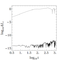
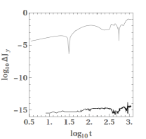
Figure 1: The left panel shows the relative error of $\Delta J_{x}$, and the right of $\Delta J_{y}$ as a function of time in logarithmic scale for the Schwarzschild background. The gray lines show the relative error of these quantities when the system is evolved using the Hamiltonian function corresponding to the tetrad (30), while the black lines show the relative error of these quantities when the system is evolved using the respective MP equations. Both evolutions share the same initial conditions conditions, where $a=0$, $M=m=1$, and $S=1$.

Generally, according to Noether’s theorem each spacetime symmetry is related to a conserved quantity. In the case of spinning particles moving in a particular spacetime geometry equipped with a symmetry described by a Killing vector $\xi_{\mu}$, the associated quantity conserved by MP equations reads

$$C=p^{\mu}\xi_{\mu}-\frac{1}{2}S^{\mu\nu}\xi_{\mu;\nu}\leavevmode\nobreak\ \leavevmode\nobreak\ .$$ (33)

In Schwarzschild spacetime we have three spatial Killing vectors yielding the three components of the total angular momentum Suzuki97

$$J_{x}= -p_{\theta}\sin\left(\phi\right)-p_{\phi}\cot\left(\theta\right)\cos\left(\phi\right)$$

$$+r^{2}S^{\theta\phi}\sin\left(\theta\right)^{2}\cos\left(\phi\right)+rS^{\phi r}\sin\left(\theta\right)\cos\left(\theta\right)\cos\left(\phi\right)$$

$$-rS^{r\theta}\sin\left(\phi\right)\leavevmode\nobreak\ \leavevmode\nobreak\ ,$$

$$J_{y}= p_{\theta}\cos\left(\phi\right)-p_{\phi}\cot\left(\theta\right)\sin\left(\phi\right)+r^{2}S^{\theta\phi}\sin\left(\theta\right)^{2}\sin\left(\phi\right)$$

$$+rS^{\phi r}\sin\left(\theta\right)\cos\left(\theta\right)\sin\left(\phi\right)+rS^{r\theta}\cos\left(\phi\right)\leavevmode\nobreak\ \leavevmode\nobreak\ ,$$

$$J_{z}= p_{\phi}-r\sin\left(\theta\right)^{2}\left(S^{\phi r}-rS^{\theta\phi}\cot\left(\theta\right)\right)\leavevmode\nobreak\ \leavevmode\nobreak\ ,$$

where $p_{i}$ are the kinematical momenta and $S^{ij}$ the spin components written in coordinate basis. In order to check whether the components of the total angular momentum are constants of motion within the Hamiltonian formulation we have to transform the expression to canonical variables $P_{i}$ and $S_{I}^{BL}$ with the relations given in (8) and (15). Therewith we obtain

$$J_{x} =\cos(\phi)(S_{1}^{BL}\csc(\theta)-P_{\phi}\cot(\theta))-P_{\theta}\sin(\phi)\leavevmode\nobreak\ \leavevmode\nobreak\ ,$$

$$J_{y} =P_{\theta}\cos(\phi)+\sin(\phi)(S_{1}^{BL}\csc(\theta)-P_{\phi}\cot(\theta))\leavevmode\nobreak\ \leavevmode\nobreak\ ,$$

$$J_{z} =P_{\phi}\leavevmode\nobreak\ \leavevmode\nobreak\ ,$$

for the components of the total angular momentum, with which we may now compute the evolution equations for $J_{i}$ via the Dirac brackets with the Hamiltonian. Indeed, they result in

$$\left\{J_{x},H\right\}_{DB} =\mathcal{O}\left(S^{2}\right)\leavevmode\nobreak\ \leavevmode\nobreak\ ,$$

$$\left\{J_{y},H\right\}_{DB} =\mathcal{O}\left(S^{2}\right)\leavevmode\nobreak\ \leavevmode\nobreak\ ,$$

$$\left\{J_{z},H\right\}_{DB} =0\leavevmode\nobreak\ \leavevmode\nobreak\ ,$$

and

$$\left\{J_{x}^{2}+J_{y}^{2}+J_{z}^{2},H\right\}_{DB} =\mathcal{O}\left(S^{2}\right)\leavevmode\nobreak\ \leavevmode\nobreak\ .$$

Although we consistently keep the linearization in the Hamiltonian and the corresponding bracket structure, we find that the Dirac brackets for $J_{x}$, $J_{y}$ and $J_{z}$ contain contributions from higher orders in the particle’s spin. Indeed, $J_{x}$ and $J_{y}$ start oscillating when the Hamiltonian system corresponding to the tetrad field (30) is numerically evolved through the the equations of motion (20)-(22). It is visible from the relative error

$$\Delta J_{i}=|1-\frac{J_{i}(t)}{J_{i}(0)}|\leavevmode\nobreak\ \leavevmode\nobreak\ \leavevmode\nobreak\ i=x,y\leavevmode\nobreak\ \leavevmode\nobreak\ ,$$ (34)

at time $t$ of the $J_{x}$ and $J_{y}$ (gray line) in Fig. 1, that the Hamiltonian function resulting from the tetrad (30) apparently violates the symmetry properties of the Schwarzschild spacetime. Consequently, the total angular momentum $J^{2}$ is not preserved, because the $x$ and $y$ components of the total angular momentum exhibit inappropriate behavior. On the other hand, the respective evolution using the MP equation supplemented with NW SSC, instead, shows the expected preservation of the angular momentum components (black curves in Fig. 1). This shows that even in the above linear in spin Hamiltonian approximation a quantity is a constant of motion only when its Dirac brackets with the Hamiltonian are exactly zero, while when the brackets have contributions from the higher in spin orders, the quantities show no constancy. The violation of the expected symmetries results in a system that exhibits chaotic motion (scattered dots in the left panel of Fig. 2), which contradicts with the integrability of the Hamiltonian for the spinning particle on the Schwarzschild background we prove in section III.2. It is true, however, that the relative error of the $J_{x},\leavevmode\nobreak\ J_{y}$ components, and therefore of $J^{2}$ scale with $S$ (right panel of Fig. 2). However, this should be anticipated since as $S\rightarrow 0$ the system basically ignores the spin contribution and tends to reproduce geodesic trajectories.

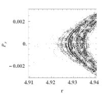
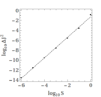
Figure 2: In the left panel is a detail from the surface of section $\theta=\pi/2$, $P_{\theta}>0$. The parameters of the orbits are $H=0.95$, $J_{z}=P_{\phi}=3$, $S=M=m=1$, $a=0$, the common initial conditions are $\phi=0$, $P_{r}=0$, $S_{1}=S_{2}=0$, $S=S_{3}=10^{-2}$, while the initial $P_{\theta}$ is defined numerically by the Hamiltonian function $H$. The right panel shows how the maximal value of the relativity error $\Delta J^{2}=|1-J^{2}(t)/J^{2}(0)|$ for evolution intervals $t=10^{3}$ scales with the spin measure $S$.

In this work we focus on the properties of the equations of motion, and not so much on the astrophysical implication of these equations. The spin of the particle makes the trajectories to deviate from their geodesic paths. Thus, we can interpret the spin as a perturbation parameter of the system. A constant of motion cannot dependent on the magnitude of the spin, even if the given value might be astrophysically irrelevant. This independence from the spin magnitude holds also for the integrability of a spinning particle Hamiltonian (excluding of course the case when $S=0$). In our numerical calculations we measure the spin in units of $m\leavevmode\nobreak\ M$, i.e. $\sigma=S/(m\leavevmode\nobreak\ M)$, and set both masses to $1$, thus the spin parameter $\sigma=S$ is dimensionless. Large values of the dimensionless spin, like $S=1$, might be astrophysically questionable, but do not have implications on the dynamics (see, e.g., Suzuki97 ; Hartl03a for relevant discussions). In our paper large values of the spin serve mainly as a tool to amplify the effects we want to point out, since these effects become less prominent when $S\ll 1$.

Moreover, we find that

$$\left\{L_{x}^{2}+L_{y}^{2}+L_{z}^{2},H\right\}_{DB}=\mathcal{O}\left(S^{2}\right)\leavevmode\nobreak\ \leavevmode\nobreak\ ,$$

with

$$L_{x} =-p_{\theta}\sin(\phi)-p_{\phi}\cot(\theta)\cos(\phi)\leavevmode\nobreak\ \leavevmode\nobreak\ ,$$

$$L_{y} =p_{\theta}\cos(\phi)-p_{\phi}\cot(\theta)\sin(\phi)\leavevmode\nobreak\ \leavevmode\nobreak\ ,$$

$$L_{z} =p_{\phi}\leavevmode\nobreak\ \leavevmode\nobreak\ ,$$

which also have to be rewritten in terms of the canonical momenta $P_{i}$. The conservation of the measure of the orbital momentum $L^{2}$ of the linearized in spin MP equation in the case of the Schwarzschild spacetime background has been thoroughly discussed in Apostolatos96 for the Pirani SSC Pirani56 . When the measure of the spin $S^{2}=S_{I}S^{I}$ and the total angular momentum $J^{2}$ are preserved, the integral of motion $L^{2}$ is equivalent to the conservation of $\vec{L}\cdot\vec{S}$. However, as in the case of the total angular momentum, we recover the same numerical problems for the measure of the orbital angular momentum. These two oscillations issues can be traced back to the coordinate dependence of the basis vectors in the spherical coordinate system, as we will see in the next subsection.

So far, these coordinate effects have been investigated in Schwarzschild spacetime. Since the Schwarzschild spacetime is the nonrotating limit of the Kerr spacetime we would like to ensure that such coordinate effects can be eliminated in the nonrotating limit, i.e., the coordinate effects should vanish for nonrotating or slowly rotating black holes. Thus, we were wondering whether there are more suitable choices of a coordinate system and of a tetrad for rotating black holes which do not show any unphysical coordinate effects in the Schwarzschild limit. Hence, the question arises as to which coordinates are best used?

Therefore, in the rest of Sec. III we study the Hamiltonian formulation in an isotropic coordinate systems for the same kind of observer (ZAMO), introduced by Barausse10 .

III.2 The Hamiltonian function in isotropic Cartesian coordinates

A revised Hamiltonian function for the Kerr spacetime background in BL has been provided in Barausse10 . The formulation starts in Cartesian quasi-isotropic coordinates. The line element in these coordinates for an axisymmetric stationary metric is

$$ds^{2} = g_{tt}\leavevmode\nobreak\ dt^{2}$$ (35)

$$+ 2\leavevmode\nobreak\ g_{tX}dX\leavevmode\nobreak\ dt+2\leavevmode\nobreak\ g_{tY}dY\leavevmode\nobreak\ dt+2\leavevmode\nobreak\ g_{XY}dX\leavevmode\nobreak\ dY$$

$$+ g_{XX}\leavevmode\nobreak\ dX^{2}+g_{YY}\leavevmode\nobreak\ dY^{2}+g_{ZZ}\leavevmode\nobreak\ dZ^{2}\leavevmode\nobreak\ \leavevmode\nobreak\ ,$$

with

$$g_{tt} = e^{-2\nu}\left[B^{2}\omega^{2}(X^{2}+Y^{2})-e^{4v}\right]\leavevmode\nobreak\ \leavevmode\nobreak\ ,$$

$$g_{tX} = e^{-2\nu}\omega B^{2}Y\leavevmode\nobreak\ \leavevmode\nobreak\ ,$$

$$g_{tY} = -e^{-2\nu}\omega B^{2}X\leavevmode\nobreak\ \leavevmode\nobreak\ ,$$

$$g_{XY} = -\frac{(e^{-2\nu}B^{2}-e^{2\mu})XY}{X^{2}+Y^{2}}\leavevmode\nobreak\ \leavevmode\nobreak\ ,$$

$$g_{XX} = \frac{e^{2\mu}X^{2}+e^{-2\nu}B^{2}\leavevmode\nobreak\ Y^{2}}{X^{2}+Y^{2}}\leavevmode\nobreak\ \leavevmode\nobreak\ ,$$

$$g_{YY} = \frac{e^{2\mu}Y^{2}+e^{-2\nu}B^{2}\leavevmode\nobreak\ X^{2}}{X^{2}+Y^{2}}\leavevmode\nobreak\ \leavevmode\nobreak\ ,$$

$$g_{ZZ} = e^{2\mu}\leavevmode\nobreak\ \leavevmode\nobreak\$$ (36)

where $\omega,\,e^{\mu},\,e^{\nu},\,B$ are functions of $X,\,Y,\,Z$.

For this coordinate system the authors propose the tetrad field

$$\tilde{e}_{\beta}\,^{T} = e^{\nu}\delta_{\beta}^{t}\leavevmode\nobreak\ \leavevmode\nobreak\ ,$$

$$\tilde{e}_{\beta}\,^{1} = \frac{B\leavevmode\nobreak\ \omega\leavevmode\nobreak\ Y}{e^{\nu}}\delta_{\beta}^{t}+\frac{e^{\mu}X^{2}+e^{-\nu}B\leavevmode\nobreak\ Y^{2}}{X^{2}+Y^{2}}\delta_{\beta}^{X}$$

$$+ \frac{(e^{\mu}-e^{-\nu}B)XY}{X^{2}+Y^{2}}\delta_{\beta}^{Y}\leavevmode\nobreak\ \leavevmode\nobreak\ ,$$

$$\tilde{e}_{\beta}\,^{2} = -\frac{B\leavevmode\nobreak\ \omega\leavevmode\nobreak\ X}{e^{\nu}}\delta_{\beta}^{t}+\frac{(e^{\mu}-e^{-\nu}B)XY}{X^{2}+Y^{2}}\delta_{\beta}^{X}$$

$$+ \frac{e^{\mu}Y^{2}+e^{-\nu}B\leavevmode\nobreak\ X^{2}}{X^{2}+Y^{2}}\delta_{\beta}^{Y}\leavevmode\nobreak\ \leavevmode\nobreak\ ,$$

$$\tilde{e}_{\beta}\,^{3} = e^{\mu}\delta_{\beta}^{Z}\leavevmode\nobreak\ \leavevmode\nobreak\ ,$$ (37)

corresponding to an infalling observer with zero 3-momentum. This tetrad becomes Cartesian, i.e., $\tilde{e}_{\beta}\,^{T}=1$, $\tilde{e}_{\beta}\,^{I}=\delta_{\beta}^{I}$, in the flat spacetime limit.

The Cartesian quasi-isotropic coordinates relate with the BL coordinate system through the transformation

$$X = R\left(r\right)\sin{\theta}\cos{\phi}\leavevmode\nobreak\ \leavevmode\nobreak\ ,$$

$$Y = R\left(r\right)\sin{\theta}\sin{\phi}\leavevmode\nobreak\ \leavevmode\nobreak\ ,$$

$$Z = R\left(r\right)\cos{\theta}\leavevmode\nobreak\ \leavevmode\nobreak\ ,$$

$$R\left(r\right) = \frac{1}{2}(r-M+\sqrt{\Delta})\leavevmode\nobreak\ \leavevmode\nobreak\ .$$ (38)

The above relation between $r$ and $R$ holds outside the black hole’s horizon .

When we go back to the Schwarzschild spacetime where $a\rightarrow 0$,

$$ds^{2}=-f(R)dt^{2}+h(R)(dX^{2}+dY^{2}+dZ^{2})\leavevmode\nobreak\ \leavevmode\nobreak\ ,$$ (39)

the tetrad (37) reduces to the isotropic tetrad given in Barausse09 :

$$\tilde{e}_{\beta}\,^{T} = \sqrt{1-\frac{2M}{r}}\delta_{\beta}^{t}=\sqrt{f\left(R\right)}\delta_{\beta}^{t}\leavevmode\nobreak\ \leavevmode\nobreak\ ,$$

$$\tilde{e}_{\beta}\,^{1} = \frac{r}{R}\delta_{\beta}^{X}=\left(1+\frac{M}{2R}\right)^{2}\delta_{\beta}^{X}\leavevmode\nobreak\ \leavevmode\nobreak\ ,$$

$$\tilde{e}_{\beta}\,^{2} = \frac{r}{R}\delta_{\beta}^{Y}=\left(1+\frac{M}{2R}\right)^{2}\delta_{\beta}^{Y}\leavevmode\nobreak\ \leavevmode\nobreak\ ,$$

$$\tilde{e}_{\beta}\,^{3} = \frac{r}{R}\delta_{\beta}^{Z}=\left(1+\frac{M}{2R}\right)^{2}\delta_{\beta}^{Z}\leavevmode\nobreak\ \leavevmode\nobreak\ ,$$ (40)

where

$$r =R\left(1+\frac{M}{2R}\right)^{2}\leavevmode\nobreak\ \leavevmode\nobreak\ ,$$

$$f(R) =\frac{\left(2R-1\right)^{2}}{\left(2R+1\right)^{2}}\leavevmode\nobreak\ \leavevmode\nobreak\ ,$$

$$h\left(R\right) =\left(1+\frac{M}{2R}\right)^{4}\leavevmode\nobreak\ \leavevmode\nobreak\ .$$

In order to check the behavior of these so called isotropic Cartesian coordinates $\left(X,Y,Z\right)$ we analyze the conservation of the constants of motion given by the symmetries of the system. The spherical symmetry of the spacetime can be described in Cartesian-like coordinates $x^{\mu}$ by the following three Killing vectors

$${\xi}_{K}^{\mu}=\epsilon^{KLM}x^{L}\delta_{M}^{\mu}\leavevmode\nobreak\ \leavevmode\nobreak\ .$$ (41)

Using (33) we thus get the three conserved components of the total angular momentum as a combination of the kinematical momentum $p_{\mu}$ and the components of the spin tensor $S^{\mu\nu}$. On the other hand, in the canonical description, the conservation of the total angular momentum

$$J_{K}=\epsilon^{KLM}x^{L}P_{M}+S_{K}\leavevmode\nobreak\ \leavevmode\nobreak\ ,$$ (42)

is demonstrated by vanishing Dirac brackets

$$\left\{J_{K},H\right\}_{DB}=0\leavevmode\nobreak\ \leavevmode\nobreak\ .$$ (43)

Contrary to the previous case the canonical momenta $P_{M}$ and tetrad components of the spin appear in this formula. The relations between the two sets of quantities, the kinematical and the canonical, are given by (15) and (8). By computing the difference of projection of (33) and (42) it can be shown, that if the Lie derivatives of the three spatial tetrad vectors obey the Cartesian-like rule

$$\left(\pounds_{\xi_{K}}\tilde{e}^{\mu}\,_{L}\right)\tilde{e}_{\mu M}=-\epsilon_{KLM}\leavevmode\nobreak\ \leavevmode\nobreak\ \leavevmode\nobreak\ \leavevmode\nobreak\ {\rm and}\leavevmode\nobreak\ \leavevmode\nobreak\ \leavevmode\nobreak\ \leavevmode\nobreak\ \xi_{K}^{0}\equiv 0\leavevmode\nobreak\ \leavevmode\nobreak\ ,$$ (44)

the two conserved quantities, one in kinematical variables and the other in canonical ones, are identical. Indeed, this formula holds in the flat Minkowski spacetime for the Cartesian tetrad $\tilde{e}_{\mu}\,^{A}=\delta_{\mu}^{A}$, which naturally leads to the intuition, that a tetrad, that reduces to a Cartesian one in the flat spacetime, is a good tetrad choice. (In (44) the fact that the time component of the Killing vectors is required to vanish is explicitly stated, since it is written as a covariant, coordinate independent formula, but it has been derived using the above coordinate assumption.)

The general condition (44) can now be applied to the particular case of the Schwarzschild limit (39). As Lie derivatives can be written using partial rather than covariant derivatives, one can easily check, that the tetrad field (40) satisfies (44).

Yet, as an example, that the equivalence between total angular momentum expressed in kinematical and canonical variables is not so obvious, let us consider a symmetry of the Schwarzschild spacetime w.r.t. rotation along the $z$-axis

$${\xi}_{z}^{\mu}=[0,-Y,X,0]\leavevmode\nobreak\ \leavevmode\nobreak\ .$$ (45)

It yields the related component of the total angular momentum

$$J_{z}= Xp_{y}-Yp_{x}+S^{xy}\left(h\left(R\right)+\frac{\left(h\left(R\right)\right)^{\prime}}{2R}\left(X^{2}+Y^{2}\right)\right)$$

$$-\frac{\left(h\left(R\right)\right)^{\prime}}{2R}Z\left(XS^{yz}+YS^{zx}\right)\leavevmode\nobreak\ \leavevmode\nobreak\ .$$

Here, $p_{i}$ represents the kinematical MP momenta and $S^{ij}$ the coordinate spin components, the prime denotes a derivative with respect to $R$. In the Hamiltonian approach we use the canonical momenta $P_{i}$ and the projected spin components $S^{I}$, so it is necessary to perform a transformation from $\left(p_{i},S^{ij}\right)$ to $\left(P_{I},S^{I}\right)$ using the relations given in (15) and (8). By doing this, terms proportional to $h^{\prime}(R)$ get absorbed into $P_{x}$ and $P_{y}$ and the corresponding component of the total angular momentum can be written as

$$J_{z} =XP_{y}-YP_{x}+S_{3}\leavevmode\nobreak\ \leavevmode\nobreak\ .$$ (46)

The corresponding Hamiltonian in these coordinates, cf. Barausse09 reads

$${H=H_{NS}+H_{S}\leavevmode\nobreak\ \leavevmode\nobreak\ ,}$$

with

$$H_{NS} =\frac{1}{\sqrt{f\left(R\right)}}\sqrt{Q}\leavevmode\nobreak\ \leavevmode\nobreak\ ,$$ (47)

$$H_{S} =\frac{1-\frac{M}{2R}+2\left(1-\frac{M}{4R}\right)\sqrt{Q}}{\left(1+\frac{M}{2R}\right)^{6}R^{3}\sqrt{Q}\left(1+\sqrt{Q}\right)}\frac{M}{m}\left(\vec{L}\cdot\vec{S}\right)\leavevmode\nobreak\ \leavevmode\nobreak\ ,$$ (48)

and $Q=m^{2}+\frac{1}{h\left(R\right)}\vec{P}^{2}$. Notice, that setting $M\rightarrow 0$, i.e., no gravitational field, we indeed obtain that the spin part of the Hamiltonian $H_{S}$ becomes zero, as it should in the Minkowskian spacetime.

Next, we can easily compute the evolution equations for the $J_{x}$, $J_{y}$ and $J_{z}$ as

$$\left\{J_{x},H\right\}_{DB} =0\leavevmode\nobreak\ \leavevmode\nobreak\ ,$$

$$\left\{J_{y},H\right\}_{DB} =0\leavevmode\nobreak\ \leavevmode\nobreak\ ,$$

$$\left\{J_{z},H\right\}_{DB} =0\leavevmode\nobreak\ \leavevmode\nobreak\ ,$$

which is thus also true for the measure of the total angular momentum $J^{2}$. Moreover, it holds that $\left\{L^{2},H\right\}=0$ where $L^{2}=L_{x}^{2}+L_{y}^{2}+L_{z}^{2}$ is the measure of the orbital angular momentum. Its respective components are defined as $L_{i}=\varepsilon_{ijk}q^{j}P^{k}$, with $q^{i}=\left(X,Y,Z\right)$ and $P^{i}=\left(P_{x},P_{y},P_{z}\right)$.

In fact, since the linearized in spin Hamiltonian system given by (47), (48) has five degrees of freedom, the five independent and in involution constants of motion $(J_{z},J^{2},L^{2},S^{2},H)$ of the Schwarzschild limit make the system integrable. The integrability for the Schwarzschild background seems to result from the linearized in spin Hamiltonian approximation, because in Suzuki97 it has been shown that for the full MP equations with T SSC chaos appears for a spinning particle moving in the Schwarzschild background. However, the integrability seems to vanish in the Hamiltonian approximation once we turn on the spin of the central body. Namely, in the case of a Kerr spacetime background chaos appears again (scattered dots in Fig. 3), which suggests the nonintegrability of the corresponding Hamiltonian system. The existence of chaos in the Kerr background case for the Hamiltonian approximation is not just a confirmation of previous studies concerning the full MP equations with T SSC, see, e.g., Hartl03a ; Hartl03b . It shows that the linearized in spin Hamiltonian function given in Barausse10 is non-integrable. This result contradicts statements in the literature saying that up to the linear order in spin the motion of a spinning particle corresponds to an integrable system, see, e.g., Hinderer13 . A thorough investigation of chaos in the Kerr spacetime for the linearized in spin Hamiltonian function will be provided in LGKPS .

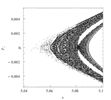
Figure 3: A detail from the surface of section $\theta=\pi/2$, $P_{\theta}>0$. The parameters of the orbits are $H=0.9449111825230683$, $J_{z}=3.5$, $S=M=m=1$, $a=0.1$, the common initial conditions are $\phi=0$, $P_{r}=0$, $S_{1}=0$, while by solving numerically the system $P_{\theta}=-S_{2}$, $J_{z}=P_{\phi}+S_{3}$, and $S=\sqrt{S_{2}^{2}+S_{3}^{2}}$ we define the rest.

The above results match exactly the expectations we had from the symmetries.

Up to this point, we have discussed the properties of a ZAMO tetrad in spherical and Cartesian coordinates in Schwarzschild spacetime. Taking the conservation of the constants of motion for numerical calculations as an important criterion to be satisfied, promising indicators for a “good” tetrad choice are the reduction to Cartesian tetrad in flat spacetime as well as the vanishing of the spin dependent Hamiltonian. Two questions arise with this statement: First, are there other coordinates we may choose providing us with “good” tetrads, and second, since we were focusing on a ZAMO tetrad, we ask whether a non-ZAMO tetrad yields the same properties if the coordinate basis is not changed. We expect the properties of the tetrad to depend on the choice of the coordinates, so that in the following we take Kerr-Schild coordinates and analyze two tetrads, one ZAMO and one non-ZAMO tetrad.

IV The Hamiltonian function in Kerr-Schild coordinates

The Kerr-Schild coordinates have the great advantage that they are horizon penetrating so that they are well behaved in the vicinity of the horizon, which simplifies numerical calculations in this domain, probably improving the numerical treatment compared to isotropic coordinates for events in the strong field. Here we shall introduce a Hamiltonian function using the Kerr-Schild (KS) coordinates. The line element in KS coordinates reads Gualtierie

$$ds^{2} = g_{\mu\nu}d\bar{x}^{\mu}d\bar{x}^{\nu}\leavevmode\nobreak\ \leavevmode\nobreak\ ,$$

$$g_{\mu\nu} = \eta_{\mu\nu}+f\leavevmode\nobreak\ l_{\mu}\leavevmode\nobreak\ l_{\nu}\leavevmode\nobreak\ \leavevmode\nobreak\ ,$$ (49)

where $(0,1,2,3)$ correspond to $(\bar{t},\bar{x},\bar{y},\bar{z})$,

$$l_{\bar{t}} = -1\leavevmode\nobreak\ \leavevmode\nobreak\ ,$$

$$l_{\bar{x}} = -\frac{\bar{r}\leavevmode\nobreak\ \bar{x}+a\leavevmode\nobreak\ \bar{y}}{\bar{r}^{2}+a^{2}}\leavevmode\nobreak\ \leavevmode\nobreak\ ,$$

$$l_{\bar{y}} = -\frac{\bar{r}\leavevmode\nobreak\ \bar{y}-a\leavevmode\nobreak\ \bar{x}}{\bar{r}^{2}+a^{2}}\leavevmode\nobreak\ \leavevmode\nobreak\ ,$$

$$l_{\bar{z}} = -\frac{\bar{z}}{\bar{r}}\leavevmode\nobreak\ \leavevmode\nobreak\ ,$$ (50)

and

$$f = \frac{2\leavevmode\nobreak\ M\leavevmode\nobreak\ \bar{r}^{3}}{\bar{r}^{4}+a^{2}\leavevmode\nobreak\ \bar{z}^{2}}\leavevmode\nobreak\ \leavevmode\nobreak\ ,$$ (52)

$$\bar{r} = \sqrt{\frac{\bar{\rho}^{2}+\sqrt{\bar{\rho}^{4}+4a^{2}\leavevmode\nobreak\ z^{2}}}{2}}\leavevmode\nobreak\ \leavevmode\nobreak\ ,$$

$$\bar{\rho}^{2} = \bar{x}^{2}+\bar{y}^{2}+\bar{z}^{2}-a^{2}\leavevmode\nobreak\ \leavevmode\nobreak\ .$$ (53)

For simplicity in the rest of the section we drop the bar notation over the KS coordinates.

Independently on the tetrad field the choice of coordinates implies the non-spinning part of the Hamiltonian

$$H_{NS}=\alpha^{2}f\leavevmode\nobreak\ l_{i}P_{i}+\alpha\sqrt{m^{2}+P_{i}P_{i}-f\alpha^{2}(l_{i}P_{i})^{2}}\leavevmode\nobreak\ \leavevmode\nobreak\ ,$$ (54)

where $l_{i}P_{i}=\delta^{ij}l_{i}P_{j}$ and

$$\alpha=\frac{1}{\sqrt{1+f}}\leavevmode\nobreak\ \leavevmode\nobreak\ .$$ (55)

In the following we present two tetrad choices corresponding to different types of observers.

IV.1 ZAMO Tetrad

In the previous section, we focused on a tetrad field associated to the observers with vanishing momenta $P_{i}=0$, i.e., zero angular momentum observers (ZAMO), in two different coordinate systems, isotropic Cartesian and Boyer-Lindquist coordinates. Therefore, it is reasonable to first consider such an observer in KS coordinates as well. Here, we choose a tetrad corresponding to an observer infalling with the radial velocity $U^{r}=-\alpha f$:

$$\tilde{e}_{\beta}\,^{T} = \alpha\;\delta_{t}^{0}\leavevmode\nobreak\ \leavevmode\nobreak\ ,$$

$$\tilde{e}_{\beta}\,^{I} = \delta_{\beta}^{I}+\left(\alpha^{-1}\!\!-1-\alpha f\right)l_{I}\,\delta_{\beta}^{0}+\left(\alpha^{-1}\!\!-1\right)l_{I}l_{\beta}\leavevmode\nobreak\ \leavevmode\nobreak\ .$$

Again, this tetrad becomes Cartesian, i.e., $\tilde{e}_{\beta}\,^{T}=\delta_{\beta}^{T}$, $\tilde{e}_{\beta}\,^{I}=\delta_{\beta}^{I}$, in the flat spacetime limit, which is a first indicator for being a good tetrad choice. The next step is to analyze the behavior in the Schwarzschild limit $a\rightarrow 0$. Then, following the procedure introduced in Barausse09 , we obtain the Hamiltonian $\bar{H}^{{\rm Schw}}=\bar{H}_{NS}^{{\rm Schw}}+\bar{H}_{S}^{{\rm Schw}}$ with

$${\bar{H}}_{NS}^{{\rm Schw}} =\alpha\left(\overline{m}-\frac{2M\alpha}{r^{2}}\;\vec{r}\!\cdot\!\vec{P}\right)\leavevmode\nobreak\ \leavevmode\nobreak\ ,$$ (56)

$${\bar{H}}_{S}^{{\rm Schw}} =\frac{M}{\overline{m}}\left[\frac{2\alpha^{2}}{\alpha+1}-\frac{\alpha^{5}+3\alpha^{3}}{r}\frac{\vec{r}\!\cdot\!\vec{P}}{\omega_{T}}-\alpha^{4}\frac{\overline{m}}{\omega_{T}}\right]\frac{\vec{L}\cdot\vec{S}}{r^{3}}\leavevmode\nobreak\ \leavevmode\nobreak\ ,$$ (57)

where

$$\overline{m} =\sqrt{m^{2}+\vec{P}^{2}-\frac{f\alpha^{2}}{r^{2}}\left(\vec{r}\!\cdot\!\vec{P}\right)^{2}}\leavevmode\nobreak\ \leavevmode\nobreak\ ,$$

$$\omega_{T} =-m-\overline{m}\leavevmode\nobreak\ \leavevmode\nobreak\ .$$ (58)

Since the total Hamiltonian is merely a function of certain scalar combinations of $\left(\vec{r},\vec{P},\vec{S}\right)$ (where $\vec{r}=\left(x,y,z\right)$), namely $\bar{H}=\bar{H}\left(|\vec{r}|^{2},|\vec{P}|^{2},\vec{r}\cdot\vec{P},\vec{L}\cdot\vec{S}\right)$ with $L_{i}=\varepsilon_{ijk}r^{j}P^{k}$ , we can deduce that

$$\left\{\vec{L}+\vec{S},H\right\}_{DB}=0\leavevmode\nobreak\ \leavevmode\nobreak\ ,$$ (59)

by using the canonical structure of the variables. Moreover, we would like to stress here again, that the conservation of $L^{2}$ in Schwarzschild spacetime is equivalent to the conservation of $\vec{L}\cdot\vec{S}$ so that it suffices to express the Hamiltonian in terms of $\vec{L}\cdot\vec{S}$ in order to show (59). In fact, it reflects the integrability of the system at linear order in spin.

However, we cannot simply infer that $\vec{J}=\vec{L}+\vec{S}$ is valid in the new canonical coordinates. The conserved total angular momentum is already given by (33) and by the Killing vectors (41) of the Schwarzschild spacetime we get

$$J_{i} =\tilde{L}_{i}+S_{i}\leavevmode\nobreak\ \leavevmode\nobreak\ ,$$ (60)

where the tilde denotes the quantities to be written in terms of the kinematical momenta $p_{i}$ $\left(L_{i}=\varepsilon_{ijk}r^{j}p^{k}\right)$ and the index $i$ in $S_{i}$ refers to the coordinate basis. This relation is valid in KS coordinates, independent of the tetrad choice.

In order to relate the conserved quantities to the canonical momenta $P_{i}$ and the tetrad components of the spin $S_{I}$, we have to perform a transformation from $\left(p_{i},S_{i}\right)$ to $\left(P_{i},S_{I}\right)$ using the relations given in (15) and (8). Therewith, we indeed find the components $J_{i}$ to be given by (46), which yields vanishing Dirac brackets for each component of the total angular momentum according to the argument mentioned in Section III.2. In order to support this statement we performed a numerical check shown in Fig. 4.

Figure 4: The left panel shows the relative error of $J_{x}$, and the right of $J_{y}$ as a function of time in logarithmic scale for the ZAMO tetrad in KS coordinates as evolved by the Hamiltonian with $a=0$, $M=m=1$, and $S=1$.

It is immediately obvious that the conservation of these components is ensured up to numerical errors which do not accumulate over the integration time but stay at the same level. These results are similar to the ones obtained in isotropic Cartesian coordinates, so that the quality of the outputs is comparable. Therefore, if one can choose between KS and isotropic Cartesian coordinates, there is no preferred choice between those two in Schwarzschild spacetime. However, if the dynamics of plunging orbits is considered in a Kerr spacetime background, it may be more sensible to change to KS coordinates since they are horizon penetrating and avoid numerical divergence close to the horizon (see Appendix B).

Second, we consider the contribution from the spin part of the Hamiltonian in flat spacetime. From (57) we see that for $M\rightarrow 0$ the contributions from $H_{S}$ vanish as it should. Hence, also additional coordinate effects which arise in spherical coordinates are avoided, further supporting such a choice of tetrad and coordinates.

IV.2 Non-ZAMO tetrad

To simplify the Hamiltonian in Kerr-Schild coordinates we change to another tetrad field, which is not required to be a ZAMO observer. In particular, we take advantage of the fact that for certain observers no square roots appear due to normalization of the tetrad vectors

$$\tilde{e}_{\mu}\,^{T} =\left[1-\frac{f}{2},\leavevmode\nobreak\ \frac{f}{2}l_{x},\leavevmode\nobreak\ \frac{f}{2}l_{y},\leavevmode\nobreak\ \frac{f}{2}l_{z}\right]\leavevmode\nobreak\ \leavevmode\nobreak\ ,$$ (61)

$$\tilde{e}_{\mu}\,^{X} =\left[\leavevmode\nobreak\ -\frac{f}{2}l_{x},\leavevmode\nobreak\ 1+\frac{f}{2}l_{x}l_{x},\leavevmode\nobreak\ \frac{f}{2}l_{x}l_{y},\leavevmode\nobreak\ \frac{f}{2}l_{x}l_{z}\right]\leavevmode\nobreak\ \leavevmode\nobreak\ ,$$ (62)

$$\tilde{e}_{\mu}\,^{Y} =\left[\leavevmode\nobreak\ -\frac{f}{2}l_{y},\leavevmode\nobreak\ \frac{f}{2}l_{y}l_{x},\leavevmode\nobreak\ 1+\frac{f}{2}l_{y}l_{y},\leavevmode\nobreak\ \frac{f}{2}l_{y}l_{z}\right]\leavevmode\nobreak\ \leavevmode\nobreak\ ,$$ (63)

$$\tilde{e}_{\mu}\,^{Z} =\left[\leavevmode\nobreak\ -\frac{f}{2}l_{z},\leavevmode\nobreak\ \frac{f}{2}l_{z}l_{x},\leavevmode\nobreak\ \frac{f}{2}l_{z}l_{y},\leavevmode\nobreak\ 1+\frac{f}{2}l_{z}l_{z}\right]\leavevmode\nobreak\ \leavevmode\nobreak\ ,$$ (64)

where we use the definitions from above, cf. Eqs. (50)-(52). This is the tetrad of an infalling ‘non-ZAMO’ observer, as the observer’s specific angular momentum

$$\tilde{e}_{\phi T}=\left(\frac{\partial}{\partial\phi}\right)^{\mu}\tilde{e}_{\mu T}=-\frac{1}{2}\,\frac{fa}{r}\frac{x^{2}+y^{2}}{r^{2}+a^{2}} \neq 0\leavevmode\nobreak\ \leavevmode\nobreak\ ,$$ (65)

and the observer’s radial coordinate velocity

$$\tilde{e}^{r}\,_{T}=\left(\frac{\partial r}{\partial x^{\mu}}\right)\tilde{e}^{\mu}\,_{T}\leavevmode\nobreak\ =-\frac{f}{2}<0\leavevmode\nobreak\ \leavevmode\nobreak\ .$$

Thus, we again compute the Hamiltonian in canonical coordinates up to linear order in spin given by Barausse09

$$H=H_{NS}+H_{SO}+H_{SS}\leavevmode\nobreak\ \leavevmode\nobreak\ ,$$ (66)

where $H_{NS}$ is given by (54),

$$H_{SO}= \leavevmode\nobreak\ \alpha f\frac{Mm-2{\widetilde{m}}(M-fr)}{2M\;\overline{m}\;\omega_{T}}\leavevmode\nobreak\ \frac{r\;\epsilon^{ijK}l_{i}p_{j}S^{K}}{r^{2}+a^{2}l_{z}^{2}}\leavevmode\nobreak\ \leavevmode\nobreak\ ,$$ (67)

and

$$H_{SS}=\leavevmode\nobreak\ -\frac{af}{4\,\omega_{T}\leavevmode\nobreak\ M{\overline{m}}\leavevmode\nobreak\ (a^{2}l_{z}^{2}+r^{2})}\times\Bigg{\{}$$ (68)

$$\Big{[}4\,{{f}{l_{z}}\,{\widetilde{m}}\left(({\overline{m}}-\alpha f{\widetilde{m}}){r}+\alpha{\widetilde{m}}M\right)}-2M\,{l_{z}}\left({\overline{m}}m+\alpha{m}^{2}\right)$$

$$\leavevmode\nobreak\ +2\,{\alpha\left[(M+{2\,r})mf{l_{z}}+(3M-2{fr})P_{z}\right]{\widetilde{m}}}\Big{]}S^{i}l_{i}$$

$$+2\,\alpha\left(m+{\widetilde{m}}\right)\left[M{l_{z}}\;{S^{i}P_{i}}-{\widetilde{m}}\left(2\,{fr}-3M\right){S^{3}}\right]$$

$$-2\,{\frac{{a}{l_{z}}\,{\widetilde{m}}}{{r}^{2}}}\left(3\,Mr-{a}^{2}f{l_{z}}^{2}-3\,f{r}^{2}\right)\Big{[}\alpha(S^{1}P_{y}-S^{2}P_{x})$$

$$-\left(\alpha m+{\overline{m}}-\alpha f{\widetilde{m}}\right)(S^{1}l_{y}-S^{2}l_{x})\Big{]}\Bigg{\}}\leavevmode\nobreak\ \leavevmode\nobreak\ .$$

Here, instead of (58), we used

$$\overline{m} =\sqrt{m^{2}+P_{i}P_{i}-f\alpha^{2}(l_{i}P_{i})^{2}}\leavevmode\nobreak\ \leavevmode\nobreak\ ,$$

$${\widetilde{m}} =\alpha\overline{m}-\alpha^{2}P_{i}l^{i}\leavevmode\nobreak\ \leavevmode\nobreak\ ,$$

$$\omega_{T} =-m-\frac{\overline{m}}{\alpha}+\frac{f}{2}\widetilde{m}\leavevmode\nobreak\ \leavevmode\nobreak\ ,$$ (69)

which together with the usage of components of $l^{\mu}$ instead of coordinates significantly shortened expressions for $H_{SO}$ and $H_{SS}$. All vector components are grouped in such a way that the relation $\left\{L_{z}+S_{z},H\right\}_{DB}=0$ is obvious.

Again, the complete angular momentum conservation is restored in the Schwarzschild limit. Since $\bar{H}_{NS}$ only depends on the chosen coordinate basis, it is still given by (56). The spinning part

$$\bar{H}_{S} =\left[\alpha\frac{M}{\overline{m}}\left(1\!-\!\frac{M+2r}{r\left(r+2M\right)}\frac{\vec{r}\!\cdot\!\vec{P}}{\omega_{T}}\right)\!-\!\frac{M}{\omega_{T}}\frac{1-\frac{M}{r}}{1+\frac{2M}{r}}\right]\frac{\vec{L}\cdot\vec{S}}{r^{3}}\leavevmode\nobreak\ \leavevmode\nobreak\ ,$$ (70)

where $\bar{m}$ and $\omega_{T}$ are given by (69), can again be written as a function $\bar{H}=\bar{H}\left(|\vec{r}|^{2},|\vec{P}|^{2},\vec{r}\cdot\vec{P},\vec{L}\cdot\vec{S}\right)$ so that we can follow the reasoning of the preceding subsection to obtain vanishing Dirac brackets (59). Therefore, we only have to check the equations for the components of the total angular momentum $J_{i}$ in canonical coordinates $\left(P_{i},S_{I}\right)$. Using the expressions for the total angular momentum with respect to the coordinate basis (60), we again perform a transformation to the tetrad basis and the canonical momenta and recover relation (46). Thus, in the Schwarzschild limit, the non-ZAMO tetrad in KS coordinates has the same numerical properties as the ZAMO tetrad, as expected, which is also visible in Fig. 5.

Figure 5: The left panel shows the relative error of $J_{x}$, and the right of $J_{y}$ as a function of time in logarithmic scale for the non-ZAMO tetrad in KS coordinates as evolved by the Hamiltonian with $a=0$, $M=m=1$, and $S=1$.

Consequently, it seems to be a good choice of coordinate system for numerical investigations.

It is of course also possible to rewrite the coefficients of the tetrad basis vectors in terms of any coordinate system without changing the general properties of the Hamiltonian system as long as the tetrad basis vectors remain oriented along the isotropic coordinate (Cartesian like) basis vectors. In Barausse09 , it was already mentioned that the coordinate effects can be avoided by choosing the directions of the tetrad basis vectors along a Cartesian coordinate system. However, if the tetrad corresponds to a Cartesian frame, the spin variables remain Cartesian whereas the position and momentum variables are spherical ones. This approach is used in effective-one-body theory or post-Newtonian methods in order to compare the dynamical contributions from different orders in spin, (see e.g., Porto06 ; Barausse09 ) and may in fact also be used for the computation of the equations of motion from the Hamiltonian. Nevertheless, in that case it is more sensible to be consistent in the choice of coordinates and spin variables so that the Dirac brackets can be used for the calculation of the equations of motion. This coordinate system does not necessarily adapt to the symmetries of the spacetime as we have seen. Generally, it is very useful to choose a coordinate system and corresponding basis vectors that do not imply coordinate effects if one aims at the analysis of the equations of motion.

V Conclusions

In this work we have studied the Hamiltonian formalism of a spinning particle provided in Barausse09 with regard to numerical investigations of the equations of motion. It was already discussed in Barausse09 that this Hamiltonian formalism does not only depend on the tetrad field one uses, but also on the coordinate system one chooses in order to express the tetrad field or the Hamiltonian function. Using the Dirac brackets to check the integrals of motion, we have shown that an unfortunate choice of the coordinate system can lead to a nonpreservation of quantities in numerical integration which should, according to the symmetries of the system and the linearized MP equations, be conserved. However, we find that the type of the tetrads, i.e., whether the observer is ZAMO or follows some other worldline which does not correspond to a ZAMO does not affect the general dynamical properties of the constants of motion. In fact, we have examined both kinds of tetrads and found no difference in their ability to be numerically applied, i.e., they possess the same properties with respect to numerical computations. However, the formulae for the spinning part of the Hamiltonian can be simplified and compactified, which we think is worthwhile to be mentioned.

In order to obtain Hamiltonian systems without coordinate effects smearing the actual physical behavior in numerical solutions and still reliable in the vicinity of the central object’s horizon, two new horizon penetrating Hamiltonian functions were introduced. Both of them were constructed on tetrad fields which were expressed in Kerr-Schild coordinates. In particular, the non-ZAMO tetrad allows us to express the Hamiltonian both in Schwarzschild and Kerr spacetime in a simple and compact form. Future (numerical) work may profit from this explicit Hamiltonian.

While studying the Dirac brackets in the Schwarzschild limit, we have shown that in this limit the Hamiltonian functions with acceptable properties are integrable. In particular, we have shown that the system’s five degrees of freedom admit five independent and in involution integrals of motion. On the other hand, we have shown by a numerical example that chaos appears when we go to the Kerr background in the case of the Hamiltonian function proposed in Barausse10 . This suggests that this linearized Hamiltonian function corresponds to a nonintegrable system in the case of the Kerr background. Indeed, the Hamiltonian formulation offers a wide range of applications in the context of chaos and perturbation theory, such as Poincaré sections or recurrence plots. In order to answer the question for chaos thoroughly, a detailed analysis of the motion of spinning particles in the Kerr spacetime described by the linearized in spin Hamiltonian approximation is in progress LGKPS .

Appendix A Numerical integration of the Hamiltonian equations

Our numerical integrators rely on the considerations of our previous work, cf. (LSK1, , Secs. A and B), which can be extended to all Hamiltonians in this work. Let us briefly summarize the main points.

All Hamiltonian equations of this work possess a so-called Poisson structure, i.e., for $\mathbf{y}=(P_{1},P_{2},P_{3},x^{1},x^{2},x^{3},S_{1},S_{2},S_{3})^{T}\in\mathbb{R}^{9}$, they can be written as

$$\dot{\mathbf{y}}=B(\mathbf{y})\mathbf{\nabla}H(\mathbf{y})\leavevmode\nobreak\ \leavevmode\nobreak\ ,$$ (71)

where $B:\mathbb{R}^{9}\to\mathbb{R}^{9\times 9}$ is the skew-symmetric matrix-valued function

$$B(\mathbf{y}) =\begin{pmatrix}0&-I_{3\times 3}&0\\ I_{3\times 3}&0&0\\ 0&0&B_{1}(\mathbf{y})\end{pmatrix}\leavevmode\nobreak\ \leavevmode\nobreak\ ,$$ (72)

with

$$I_{3\times 3} =\begin{pmatrix}1&0&0\\ 0&1&0\\ 0&0&1\end{pmatrix}\leavevmode\nobreak\ \leavevmode\nobreak\ ,$$ (73)

$$B_{1}(\mathbf{y}) =\begin{pmatrix}0&-S_{3}&S_{2}\\ S_{3}&0&-S_{1}\\ -S_{2}&S_{1}&0\end{pmatrix}\leavevmode\nobreak\ \leavevmode\nobreak\ .$$ (74)

Due to this special structure, the spin length $S=\sqrt{S_{1}^{2}+S_{2}^{2}+S_{3}^{2}}$ is conserved along solutions of the equations of motion (71). Thus, the three dimensional spin $\mathbf{S}=(S_{1},S_{2},S_{3})^{T}$ can be represented by two variables $\alpha$ and $\xi$ via

$$\mathbf{S}=S\begin{pmatrix}\sqrt{1-\xi^{2}}\cos(\alpha)\\ \sqrt{1-\xi^{2}}\sin(\alpha)\\ \xi\end{pmatrix}\leavevmode\nobreak\ \leavevmode\nobreak\ ,$$ (75)

see, e.g., wuxie ; Seyrich13 . One can then show, cf. Seyrich13 , that

$$\dot{\xi} =-\frac{\partial H}{\partial\alpha}\leavevmode\nobreak\ \leavevmode\nobreak\ ,$$ (76)

$$\dot{\alpha} =\frac{\partial H}{\partial\xi}\leavevmode\nobreak\ \leavevmode\nobreak\ ,$$ (77)

holds. Hence, in the transformed variables $\mathbf{z}=(P_{1},P_{2},P_{3},\xi,x^{1},x^{2},x^{3},\alpha)$, the equations of motion take the symplectic form

$$\dot{\mathbf{z}} =J^{-1}\mathbf{\nabla}H(\mathbf{z})\leavevmode\nobreak\ \leavevmode\nobreak\ ,$$ (78)

$$J =\begin{pmatrix}0&I_{4\times 4}\\ -I_{4\times 4}&0\end{pmatrix}\leavevmode\nobreak\ \leavevmode\nobreak\ .$$ (79)

As a nice consequence, we can evolve the system with Gauss Runge–Kutta schemes which have already been shown to yield very good results for little computational costs in previous studies, see, e.g., Seyrich13 ; SeyrichLukes12 .

An $s$-stage Gauss Runge-Kutta scheme is a collocation method, i.e., an implicit Runge-Kutta scheme

$$\mathbf{y}_{n+1} =\mathbf{y}_{n}+h\sum_{i=1}^{s}b_{i}f(\mathbf{Y}_{i})\leavevmode\nobreak\ \leavevmode\nobreak\ ,$$ (80)

$$\mathbf{Y}_{i} =\mathbf{y}_{n}+h\sum_{j=1}^{s}a_{ij}f(\mathbf{Y}_{j})\leavevmode\nobreak\ \leavevmode\nobreak\ ,\quad i=1,...,s\leavevmode\nobreak\ \leavevmode\nobreak\ ,$$ (81)

with coefficients

$$a_{ij}=\int_{0}^{c_{i}}l_{j}(t)dt\leavevmode\nobreak\ \leavevmode\nobreak\ ,$$ (82)

$$b_{j}=\int_{0}^{1}l_{i}(t)dt\leavevmode\nobreak\ \leavevmode\nobreak\ ,$$ (83)

where the stages $c_{1},...,c_{s}$ are chosen as

$$c_{i}=\frac{1}{2}(1+\tilde{c}_{i})\leavevmode\nobreak\ \leavevmode\nobreak\ ,$$ (84)

with $\tilde{c}_{i}$ being the roots of the Legendre-polynomial of degree $s$. Here, $h$ denotes the time step size, $Y_{i}$, $i=1,...,s$, are the so-called inner stage values and $\mathbf{y}_{n}$ denotes the numerical approximation to the solution $\mathbf{y}$ at time $\tau=nh$. The functions $l_{i}(t)$ are the Lagrange-polynomials of degree $s$,

$$l_{i}(t)=\prod_{i\neq j}\frac{t-c_{j}}{c_{i}-c_{j}}\leavevmode\nobreak\ \leavevmode\nobreak\ .$$ (85)

Gauss Runge-Kutta methods have a convergence order $\mathcal{O}(h^{2s})$ which is the highest possible order among collocation schemes, e.g., hairernorsettwanner . Detailed information on their implementation is given in (Seyrich13, , Sec. 7), and (hairerlubichwanner, , Chapters VIII.5 and VIII.6).

Very importantly, Gauss Runge–Kutta schemes almost exactly preserve the Hamiltonian throughout the numerical evolution, cf.(LSK1, , Fig. 10). Furthermore, it is known from numerical analysis that the solution $\mathbf{y}_{n+1}$ coincides with the value at $t=h$ of the interpolation polynomial $\mathbf{U}(t)$ through the points $(0,\mathbf{y}_{n})$ and $(c_{1},\mathbf{Y}_{1})...(c_{s},\mathbf{Y}_{s})$. This interpolation polynomial can be shown to stay $\mathcal{O}(h^{s})$ close to the exact solution of the equations of motion, see, e.g.,  (hairerlubichwanner, , Chapter II.1). Therefore, we can conveniently calculate $\mathcal{O}(h^{s})$ approximations to surface sections, such as the one presented in Fig. 3 above (for the procedure details see, e.g., Seyrich13 ).

Appendix B Plunging orbits

Figure 6: The relative error of the Hamiltonian $\Delta H$ as a function of the BL radius $r$ for two plunging orbits. The top plot shows the $\Delta H$ of a plunging orbit evolved by the Hamiltonian function discussed in section III.2 (BL), while the bottom plot shows the $\Delta H$ of a plunging orbit evolved by the Hamiltonian function discussed in section IV.2 (KS). In both cases we used masses $M=m=1$ and Kerr parameter $a=0.9$. For more about the initial conditions refer to the text. The horizon is depicted in both plots by a vertical dashed gray line.

The analytical properties of equations of motion have also an impact on the behavior of their numerical solution. In Fig. 6 we plot the relative error of the Hamiltonian $\Delta H=|1-H(t)/H(0)|$ for plunging orbits using the Gauss Runge-Kutta method (Appendix A) with fixed time step for equations of motion given by the Hamiltonian function discussed in Sec. III.2 (BL) (top plot) and the one discussed in section IV.2 (KS ) (bottom plot) as functions of the BL radius. The figure clearly shows that the KS case covers smoothly the horizon of the Kerr black hole (vertical dashed gray line), while the BL fails to do so by definition.

The mass parameters are $M=m=1$ and the Kerr parameter is $a=0.9$. As initial conditions for the BL orbit we use $r=25$, $\theta=\pi/2,\phi=0$, and $\frac{dr}{dt}=\frac{d\phi}{dt}=\frac{d\theta}{dt}=0$. The first two conditions for the velocities determine the initial values of $S_{3}$, and $P_{r}$. The remaining initial conditions are $P_{\phi}=S_{x}=S_{y}=P_{\theta}=0$. The time step is $\Delta t_{BL}=0.1$. The initial conditions for the KS orbit are $x=25,y=z=0$, and $P_{x}=P_{y}=P_{z}=0$ with spin $S_{x}=S_{z}=0,S_{z}=0.9$. The time step is $\Delta t_{KS}=0.1$.

In fact, to test how much the pole-dipole approximation of rotating body fails near the horizon has to be investigated by other studies. But, one can assume that not having equations of motion singular at the horizon helps to obtain the right numerical results within the range of spins allowed by the linear-in-spin approximation.

References

- (1) P. Amaro-Seoane, J. R. Gair, A. Pound, S. A. Hughes, and C. F.Sopuerta, J. Phys.: Conf. Ser. 610, 012002 (2015)
- (2) K. Riles, Prog. in Particle & Nuclear Phys. 68, 1 (2013)
- (3) M. Mathisson, Acta Phys. Polonica 6, 163 (1937)
- (4) A. Papapetrou, Proc. R. Soc. London Ser. A 209, 248 (1951)
- (5) O. Semerák, Mon. Not. R. Astron. S. 308, 863 (1999)
- (6) K. Kyrian, and O. Semerák, Mon. Not. R. Astron. S. 382, 1922 (2007)
- (7) C. Møller, Annales de l’I. H. P. 11, 251 (1949)
- (8) G. Lukes-Gerakopoulos, J. Seyrich, D. Kunst, Phys. Rev. D 90, 104019 (2014)
- (9) F. A. E. Pirani, Acta Phys. Polonica 15, 389 (1956)
- (10) L. F. Costa, C. Herdeiro, J. Natario and M. Zilhão, Phys. Rev. D 85, 024001 (2012).
- (11) E. Corinaldesi and A. Papapetrou, Proc. R. Soc. London Ser. A 209, 259 (1951).
- (12) O. Semerák, M. Šrámek (2015) arXiv:gr-qc/1505.01069
- (13) E. Hackmann, C. Lämmerzahl, Y. N. Obukhov, D. Puetzfeld, I. Schaffer, Phys. Rev. D 90, 064035 (2014)
- (14) R. Plyatsko, M. Fenyk, Phys. Rev. D 85, 104023 (2012).
- (15) R. Plyatsko, M. Fenyk, Phys. Rev. D 87, 044019 (2013).
- (16) S. Suzuki and K. Maeda, Phys. Rev. D 55, 4848 (1997)
- (17) M. D. Hartl, Phys. Rev. D 67, 024005 (2003).
- (18) M. D. Hartl, Phys. Rev. D 67, 104023 (2003).
- (19) C. Verhaaren, E. W. Hirschmann, Phys. Rev. D 81, 124034 (2010).
- (20) J. Steinhoff, and D. Puetzfeld, D., Phys. Rev. D 86, 044033 (2012)
- (21) D. Bini, and A. Geralico, Phys. Rev. D 89, 044013 (2014)
- (22) I. Bailey, and W. Israel, Commun. Math. Phys. 42, 65 (1975).
- (23) E. Barausse, E. Racine, and A. Buonanno, Phys. Rev. D 80, 104025 (2009)
- (24) J. Steinhoff, G. Schäfer, and S. Hergt, Phys. Rev. D 77, 104018 (2008).
- (25) J. Steinhoff, Annal. Phys 523, 296 (2011).
- (26) G. E. Tauber, International Journal of Theoretical Physics 27, 335 (1988).
- (27) A. A. Deriglazov and W. Guzmán Ramírez, arXiv:1509.04926
- (28) A. A. Deriglazov and W. Guzmán Ramírez, arXiv:1509.05357
- (29) G. Contopoulos, Order and chaos in dynamical astronomy (Springer, Berlin 2002).
- (30) R. Arnowitt, S. Deser, and C. W. Misner, in Gravitation: An Introduction to Current Research, edited by L. Witten (Wiley, New York 1962), p. 227; arXiv:gr-qc/0405109.
- (31) A. Buonanno and T. Damour, Phys. Rev. D 59, 084006 (1999).
- (32) T. Damour, P. Jaranowski, and G. Sch¨afer, Phys. Rev. D 62, 084011 (2000).
- (33) T. Damour, Int. J. Mod. Phys. A 23, 1130 (2008)
- (34) L. Blanchet, Living Rev. Rel. 9, 4 (2006).
- (35) W. Tulczyjew, Acta Phys. Polonica 18, 393 (1959)
- (36) T. D. Newton and E. P. Wigner, Rev. Mod. Phys. 21, 400 (1949)
- (37) E. Barausse, and A. Buonanno, Phys. Rev. D 81, 084024 (2010)
- (38) R. Rüdiger, Proc. R. Soc. London Ser. A 375, 185 (1981); 385, 229 (1983)
- (39) T. Hinderer, A. Buonanno, A. H. Mroué et. al, Phys. Rev. D 88,084005 (2013)
- (40) W. G. Dixon, Proc. R. Soc. London Ser. A 314, 499 (1970); Proc. R. Soc. London Ser. A 319, 509 (1970); Proc. R. Soc. London Ser. A 277, 59 (1974)
- (41) P. A. M. Dirac Canadian Journal of Mathematics 2, 129 (1950)
- (42) T. A. Apostolatos, Clas. Quant. Grav. 13, 799 (1996)
- (43) G. Lukes-Gerakopoulos, M. Katsanikas, P. Patsis and J. Seyrich, in preparation
- (44) L. Gualtierie and V. Ferrari, Lecture notes for a graduate course on black holes in general relativity (2011)
- (45) R. A. Porto, Phys. Rev. D 73, 104031 (2006).
- (46) X. Wu and Y. Xie, Phys. Rev. D 81, 084045 (2010)
- (47) J. Seyrich, Phys. Rev. D 87, 084064 (2013)
- (48) J. Seyrich and G. Lukes-Gerakopoulos, Phys. Rev. D 86, 124013 (2012)
- (49) E. Hairer, S. P. Nørsett and G. Wanner, Solving Ordinary Differential Equations I (Springer, 1993), 2nd ed.
- (50) E. Hairer, C. Lubich and G. Wanner, Geometric numerical integration. Structure-preserving algorithms for ordinary differential equations (Springer, 2006), 2nd ed.