On the ergodicity bounds for a constant retrial rate queueing model

Abstract. We consider a Markovian single-server retrial queueing system with a constant retrial rate. Conditions of null ergodicity and exponential ergodicity for the corresponding process, as well as bounds on the rate of convergence are obtained.

Key words: single-server retrial queueing system; constant retrial rate; continuous-time Markov chains; ergodicity bounds

1 Introduction

We consider the following Markovian single-server retrial queueing system with a constant retrial rate, denoted by $\Sigma$. The exogenous (primary) customers follow a Poisson input with rate $\lambda$. The customers have i.i.d. exponential service times $\{S_{i}\}$, with a generic element $S$ and rate $\mu:=1/\hbox{\sf E}S$. If a new customer finds a server busy it joins an infinite-capacity orbit and called secondary customer. We assume that the orbit works as a single FIFS (first-in, first-served or first-come, first-served) server. It means that, if the orbit is not empty, a head line (the oldest) secondary customer attempts to enter the server after an exponentially distributed time with a rate $\mu_{0}$. Thus, unlike classical retrial models, the orbit rate in $\Sigma$ does not depend on the orbit size, i.e., the number of secondary customers. Such a model is called a retrial model with constant retrial rate. Thus, orbit can be interpreted as a single-server $\cdot/M/1$-type queue with service rate $\mu_{0}$, and input is generated by the customers rejected in busy server. Note that the only possible source of instability of such system is an infinite growth of the orbit size. A sufficient stability condition of the general single-class retrial system with constant retrial rate described above is obtained in [5]. Stability analysis of multi-class retrial system is presented in [6].

Considered system can be successfully applied to model the standard multi-access protocol ALOHA, with restrictions for the individual retrial rates and has other several applications. We list the most important papers related to motivation of presented model. In [10] Fayolle first used a retrial queue with constant retrial rate to simulate a telephone exchange system. Then, in [7] the authors have modelled an unslotted Carrier Sense Multiple Access with Collision Detection (CSMA/CD) protocol and in [8] and [9] the authors have modelled some particular versions of the ALOHA protocol. The model of Fayolle [10] was extended in [1], [2] for more complex settings, such as multiple servers and waiting places. In [12] it has been proposed to use the retrial queue with constant retrial rate to model a logistic system. In [3] and [4] the authors have suggested to use retrial queues and retrial networks with constant retrial rates to model TCP traffic originated from short HTTP connections. The present retrial model also appears to be relevant for the optical-electrical hybrid contention resolution scheme for Optical Packet Switching networks [13, 14].

In this note we firstly consider the description of the model (Section 2). In Section 3, we present the auxiliary results that were obtained for birth-death processes in [11, 15, 16]. In Sections 4, 5 we apply this approach for the considered model and obtain explicit bounds on the rate of convergence both for null ergodic and exponentially ergodic situations.

2 Description of the model

Now we describe the model in more detail. For a moment $t$, let $\nu(t)$ be the number of customers in the server and $N(t)$ be the number of customers in the orbit. That is, $\nu(t)=0$, if the server is empty, and $\nu(t)=1$, otherwise, while $N(t)=0,\,1,\,\dots$. We introduce the basic two-dimensional process $X(t)=\{\nu(t),\,N(t),\,t\geq 0\}$ with the state space $\{0,\,1\}\times\{0,\,1,\,2,\,\dots\}$. Consider in more detail the transitions between the states of the system. To this end, we first enumerate the states of the process as follows: each state $\{0,\,n\}$ will be denoted $2n+1$, for $n\geq 0$, while each state $\{1,\,n\}$ is denoted $2n,\,n\geq 1$. Denote by $Q=(q_{ij})$ an intensity matrix corresponding to the given enumeration. Then it follows that

$$q_{1,1} = -\lambda,$$

$$q_{1,2} = \lambda,$$

and, for $n\geq 1$,

$$q_{2n,2n} = -(\lambda+\mu),$$

$$q_{2n,2n+2} = \lambda,$$

$$q_{2n,2n-1} = \mu,$$

$$q_{2n+1,2n+1} = -(\lambda+\mu_{0}),$$

$$q_{2n+1,2n} = \mu_{0},$$

$$q_{2n+1,2n+2} = \lambda.$$

As a result, an intensity matrix $Q=(q_{ij})$ takes the form

$$Q=\begin{pmatrix}-\lambda&\lambda&0&0&0&0&0&0&0&\cdots\\ \mu&-(\lambda+\mu)&0&\lambda&0&0&0&0&0&\cdots\\ 0&\mu_{0}&-(\lambda+\mu_{0})&\lambda&0&0&0&0&0&\cdots\\ 0&0&\mu&-(\lambda+\mu)&0&\lambda&0&0&0&\cdots\\ 0&0&0&\mu_{0}&-(\lambda+\mu_{0})&\lambda&0&0&0&\cdots\\ 0&0&0&0&\mu&-(\lambda+\mu)&0&\lambda&0&\cdots\\ \vdots&\vdots&\vdots&\vdots&\vdots&\vdots&\vdots&\vdots&\vdots&\vdots\end{pmatrix}.$$

Figures 1,2 illustrate these transitions by different but equivalent ways:

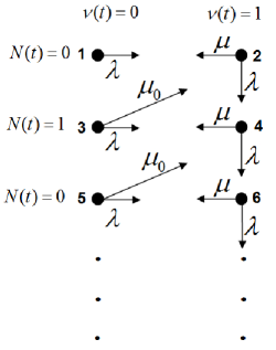
Figure 1:

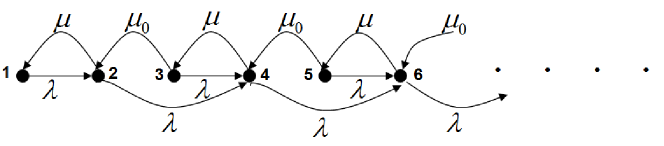
Figure 2:

3 Auxiliary notions

Then the probabilistic dynamics of the process is represented by the forward Kolmogorov system:

$$\frac{d{\mathbf{p}}}{dt}=A{\mathbf{p}},$$ (1)

where $A=\left(a_{ij}\right)_{i,j=1}^{\infty}=\left(q_{ji}\right)_{i,j=1}^{\infty}=Q^{T}$ is the corresponding transposed intensity matrix, and ${\mathbf{p}}={\mathbf{p}}(t)=\left(p_{1}(t),p_{2}(t),\dots\right)^{T}$ is the column vector of state probabilities of the process $X(t)$.

Throughout the paper by $\|\cdot\|$ we denote the $l_{1}$-norm, i. e. $\|{{\mathbf{x}}}\|=\sum|x_{i}|$, and $\|B\|=\sup_{j}\sum_{i}|b_{ij}|$ for matrix $B=(b_{ij})_{i,j=1}^{\infty}$.

We recall here the approach for the study on the rate of convergence of birth-death process, see all details and discussion in [11, 15, 16, 18].

Let $B$ be a bounded linear operator on a Banach space ${\cal B}$ and let $I$ denote the identity operator. The number

$$\gamma\left(B\right)_{\cal B}=\lim\limits_{h\rightarrow+0}\frac{\left\|I+hB\right\|-1}{h}$$

is called the logarithmic norm of $B.$

If ${\cal B}=l_{1}$, so that the operator $B$ is given by the matrix $B=\left(b_{ij}\right)_{i,j=1}^{\infty}$, then the logarithmic norm of $B$ can be found explicitly:

$$\gamma\left(B\right)_{1}=\sup\limits_{j}\left(b_{jj}+\sum\limits_{i\neq j}\left|b_{ij}\right|\right).$$

On the other hand, the logarithmic norm of the operator $B$ is related to the Cauchy operator $V(t,s)$ of differential equation

$$\frac{d{\bf x}}{dt}=B{\bf x}$$

in the following way

$$\gamma\left(B\right)_{\cal B}=\lim\limits_{h\rightarrow+0}\frac{\left\|V\left(t+h,t\right)\right\|-1}{h},\quad t\geq 0.$$

From the latter one can deduce the following bounds of the Cauchy operator $V(t,s)$, see [11, 15, 16]:

$$\left\|V\left(t,s\right)\right\|_{\cal B}\leq e^{(t-s)\gamma\left(B\right)},\quad 0\leq s\leq t.$$

Let $\Omega$ be a set of all stochastic vectors, i. e. $l_{1}$ vectors with nonnegative coordinates and unit norm. Hence $\|A\|=2\lambda+2\max(\mu,\mu_{0})<\infty$. Thus, the Cauchy problem for differential equation (1) has a unique solutions for an arbitrary initial condition, and ${\mathbf{p}}(s)\in\Omega$ implies ${\mathbf{p}}(t)\in\Omega$ for $t\geq s\geq 0$.

4 Null ergodicity

We recall that a Markov chain $X(t)$ is called null ergodic (in other terms, it means null recurrence or transience), if $p_{k}(t)\to 0$ as $t\to\infty$ for any initial condition ${\bf p}(0)$ and any $k$.

Consider a decreasing sequence of positive numbers $\{\delta_{i}\}$, $i=1,2,\dots$, and the corresponding diagonal matrix $\Delta$ with diagonal entries $\{\delta_{k}\}$.

Let $l_{1\Delta}$ be the space of sequences:

$$l_{1\Delta}=\left\{{\bf p}=(p_{1},p_{2},\cdots)^{T}:\,\|{\bf p}\|_{1\Delta}\equiv\|\Delta{\bf p}\|<\infty\right\}.$$

Then we have

$$\gamma\left(A\right)_{1\Delta}=\gamma\left(\Delta A\Delta^{-1}\right)_{1}=\sup_{i}\left(a_{ii}+\sum_{j\neq i}\frac{\delta_{j}}{\delta_{i}}a_{ji}\right).$$ (2)

Put $\delta_{1}=1$ and $\delta_{2k+1}=a\delta_{2k}$, $\delta_{2k}=b\delta_{2k-1}$, if $k\geq 1$ for some $a,b$. Then $\delta_{2k+1}=a^{k}b^{k}$, $\delta_{2k}=a^{k-1}b^{k}$, if $k\geq 1$.

We have

$$A=Q^{T}=\begin{pmatrix}-\lambda&\mu&0&0&0&0&0&0&0&\cdots\\ \lambda&-(\lambda+\mu)&\mu_{0}&0&0&0&0&0&0&\cdots\\ 0&0&-(\lambda+\mu_{0})&\mu&0&0&0&0&0&\cdots\\ 0&\lambda&\lambda&-(\lambda+\mu)&\mu_{0}&0&0&0&0&\cdots\\ 0&0&0&0&-(\lambda+\mu_{0})&\mu&0&0&0&\cdots\\ 0&0&0&\lambda&\lambda&-(\lambda+\mu)&\mu_{0}&0&0&\cdots\\ \vdots&\vdots&\vdots&\vdots&\vdots&\vdots&\vdots&\vdots&\vdots&\vdots\end{pmatrix},$$

and

$$\Delta A\Delta^{-1}=\begin{pmatrix}-\lambda&b^{-1}\mu&0&0&0&0&0&0&0&\cdots\\ b\lambda&-(\lambda+\mu)&a^{-1}\mu_{0}&0&0&0&0&0&0&\cdots\\ 0&0&-(\lambda+\mu_{0})&b^{-1}\mu&0&0&0&0&0&\cdots\\ 0&ab\lambda&b\lambda&-(\lambda+\mu)&a^{-1}\mu_{0}&0&0&0&0&\cdots\\ 0&0&0&0&-(\lambda+\mu_{0})&b^{-1}\mu&0&0&0&\cdots\\ 0&0&0&ab\lambda&b\lambda&-(\lambda+\mu)&a^{-1}\mu_{0}&0&0&\cdots\\ \vdots&\vdots&\vdots&\vdots&\vdots&\vdots&\vdots&\vdots&\vdots&\vdots\end{pmatrix}.$$

Therefore

$$\gamma\left(A\right)_{1\Delta}=-\min\left(\lambda(1-b),\lambda(1-ab)-\mu(b^{-1}-1),\lambda(1-b)-\mu_{0}(a^{-1}-1)\right)=$$

$$-\min\left(\lambda(1-ab)-\mu(b^{-1}-1),\lambda(1-b)-\mu_{0}(a^{-1}-1)\right).$$ (3)

Let now

$$\mu\mu_{0}<\lambda(\lambda+\mu_{0}).$$ (4)

Then one has

$$b^{*}:=\frac{\mu(\lambda+\mu_{0})}{\lambda(\lambda+\mu+\mu_{0})}<1.$$ (5)

Now for any $b\in(b^{*},1)$ the inequality

$$\frac{\mu_{0}}{\lambda(1-b)+\mu_{0}}<\frac{\lambda-\mu(b^{-1}-1)}{b\lambda}$$ (6)

holds.

Choose now

$$a\in\left(\frac{\mu_{0}}{\lambda(1-b)+\mu_{0}},\frac{\lambda-\mu(b^{-1}-1)}{b\lambda}\right).$$ (7)

Then $a<1,b<1$, $\lambda(1-ab)-\mu(b^{-1}-1)>0$, $\lambda(1-b)-\mu_{0}(a^{-1}-1)>0$.

Hence inequality $\gamma\left(A\right)_{1\Delta}<0$ implies null ergodicity of $X(t)$, and we obtain the following statement.

Theorem 1

Let assumption (4) hold. Then the process $X(t)$ is null ergodic and

$$\sum_{i=0}^{N}p_{i}(t)\leq\frac{\delta_{k}}{\delta_{N}}e^{-\zeta^{*}t},$$ (8)

for any $t\geq 0$, any initial condition $X(0)=k$, and any natural $N$, where

$$\zeta^{*}=\min\left(\lambda(1-ab)-\mu(b^{-1}-1),\lambda(1-b)-\mu_{0}(a^{-1}-1)\right)>0.$$

5 Exponential ergodicity

By introducing $p_{1}(t)=1-\sum_{i\geq 2}p_{i}(t)$, from (1) we obtain the equation

$$\frac{d{\mathbf{z}}}{dt}=B{\mathbf{z}}+{\mathbf{f}},$$ (9)

where ${\mathbf{f}}=\left(a_{21},a_{31},\ldots\right)^{T}=\left(\lambda,0,0,\ldots\right)^{T}$, ${\mathbf{z}}={\mathbf{z}}(t)=\left(p_{2}(t),p_{3}(t),\cdots\right)^{T}$,

$${B=\left(b_{ij}\right)_{i,j=1}^{\infty}=\left(\begin{array}[]{ccccc}a_{22}-a_{21}&a_{23}-a_{21}&\cdots&a_{2r}-a_{21}&\cdots\\ a_{32}-a_{31}&a_{33}-a_{31}&\cdots&a_{3r}-a_{31}&\cdots\\ \cdots&\cdots&\cdots&\cdots&\cdots\\ a_{r2}-a_{r1}&a_{r3}-a_{r1}&\cdots&a_{rr}-a_{r1}&\cdots\\ \cdots&\cdots&\cdots&\cdots&\cdots\end{array}\right),}$$ (10)

see detailed discussion in [15, 16, 18]. Let $\{d_{i}\}$, $i=2,3,\dots$, be a sequence of positive numbers. Put $g_{i}=\sum_{n=2}^{i}d_{n}.$

Let $D$ be the upper triangular matrix,

$$D=\left(\begin{array}[]{ccccccc}d_{2}&d_{2}&d_{2}&\cdots\\ 0&d_{3}&d_{3}&\cdots\\ 0&0&d_{4}&\cdots\\ &\ddots&\ddots&\ddots\\ \end{array}\right),$$ (11)

and $l_{1D}$ be the corresponding space of sequences

$$l_{1D}=\left\{{\bf z}=(p_{2},p_{3},\cdots)^{T}|\,\|{\bf z}\|_{1D}\equiv\|D{\bf z}\|_{1}<\infty\right\}.$$

Consider equation (9) in the space $l_{1D}$. Then the logarithmic norm $\gamma({B})_{1D}=\gamma(DBD^{-1})_{1}$, see [11, 16].

We have

$$DBD^{-1}=\begin{pmatrix}-(\lambda+\mu)&\frac{d_{2}}{d_{3}}\mu&0&0&0&0&0&0&0&\cdots\\ \frac{d_{3}}{d_{2}}\lambda&-(\lambda+\mu_{0})&\frac{d_{3}}{d_{4}}\mu_{0}&0&0&0&0&0&0&\cdots\\ \frac{d_{4}}{d_{2}}\lambda&0&-(\lambda+\mu)&\frac{d_{4}}{d_{5}}\mu&0&0&0&0&0&\cdots\\ 0&0&\frac{d_{5}}{d_{4}}\lambda&-(\lambda+\mu_{0})&\frac{d_{5}}{d_{6}}\mu_{0}&0&0&0&0&\cdots\\ 0&0&\frac{d_{6}}{d_{4}}\lambda&0&-(\lambda+\mu)&\frac{d_{6}}{d_{7}}\mu&0&0&0&\cdots\\ \vdots&\vdots&\vdots&\vdots&\vdots&\vdots\vdots&\vdots&\vdots&\vdots\\ \vdots&\vdots&\vdots&\vdots&\vdots&\vdots&\vdots&\vdots&\vdots&\vdots\end{pmatrix}.$$

Put $d_{2}=1$ and $d_{2k+1}=bd_{2k}$, $d_{2k+2}=ad_{2k+1}$, if $k\geq 1$.

Then

$$\gamma\left(B\right)_{1D}=-\inf_{i\geq 2}\alpha_{i},$$ (12)

where

$$\begin{array}[]{ccc}\alpha_{2}=\lambda+\mu-\lambda(b+ab),\\ \alpha_{2k+1}=\lambda+\mu_{0}-\mu b^{-1},\quad k\geq 1,\\ \alpha_{2k+2}=\lambda+\mu-\lambda(b+ab)-\mu_{0}a^{-1},\quad k\geq 1.\end{array}$$ (13)

Hence exponential ergodicity of the process $X(t)$ follows from the bound

$$\inf_{i\geq 1}\alpha_{i}=\min\left(\lambda+\mu_{0}-\mu b^{-1},\lambda+\mu-\lambda(b+ab)-\mu_{0}a^{-1}\right)>0,$$ (14)

for some $a,b$ such that $ab>1$, see [11, 15, 16].

Let now that

$$\mu\mu_{0}>\lambda(\lambda+\mu_{0}),$$ (15)

in contrast to (4)

Put $x=ab$.

Then one has

$$x^{*}:=\frac{\mu\mu_{0}}{\lambda(\lambda+\mu_{0})}>1.$$ (16)

Then for any $x\in(1,x^{*})$ the inequality

$$\frac{\mu}{\lambda+\mu_{0}}<\frac{\lambda+\mu-x\lambda}{\lambda+\mu_{0}/x}.$$ (17)

holds.

Choose now

$$b\in\left(\frac{\mu}{\lambda+\mu_{0}},\frac{\lambda+\mu-x\lambda}{\lambda+\mu_{0}/x}\right),$$ (18)

and $a=x/b$.

Then $\lambda+\mu_{0}-\mu b^{-1}>0,$ $\lambda+\mu-\lambda(b+ab)-\mu_{0}a^{-1}>0$, and as a result, we obtain the following statement.

Theorem 2

Let assumption (15) be true. Then the process $X(t)$ is exponentially ergodic and the following bound holds:

$$\|{\bf p}(t)-{\bf\pi}\|_{1}\leq 4e^{-\alpha^{*}t}\sum_{i\geq 2}g_{i}|p_{i}(0)-\pi_{i}|,$$ (19)

for any $t\geq 0$, and any initial condition ${\bf p}(0)$, where

$$\alpha^{*}=\min\left(\lambda+\mu_{0}-\mu b^{-1},\lambda+\mu-\lambda(b+ab)-\mu_{0}a^{-1}\right)>0,$$

and ${\bf\pi}=\left(\pi_{0},\pi_{1},\dots\right)^{T}$ is the corresponding stationary distribution.

Remark 1

It is worth mentioning that condition (15) is the stability criteria of the system studied by regenerative method in [5]. More exactly, under this condition, the workload and queue size processes are positive recurrent regenerative (that is, the mean regeneration period is finite).

Remark 2

One can obtain the respective perturbation bounds applying Theorem 2 and approach of [17]. On the other hand, the opposite condition (4) implies an unlimited growth of the process, and it is consistent with the null ergodicity which established in Theorem 1.

6 Acknowledgement

The research is supported by the Russian Foundation for Basic Research, projects no. 15-01-01698,15-07-02341,15-37-20851; and by Ministry of Education and Science, State Contract No. 1816.

References

References

• [1] Artalejo, J.R. 1996. Stationary analysis of the characteristics of the $M/M/2$ queue with constant repeated attempts. Opsearch, 33, 83–95.
• [2] Artalejo, J.R., Gómez-Corral, A.,Neuts, M.F. 2001. Analysis of multiserver queues with constant retrial rate. European Journal of Operational Research, 135, 569–581.
• [3] Avrachenkov, K., Yechiali, U. 2008. Retrial networks with finite buffers and their application to Internet data traffic. Probability in the Engineering and Informational Sciences, 22, 519–536.
• [4] Avrachenkov, K., Yechiali, U. 2010. On tandem blocking queues with a common retrial queue. Computers and Operations Research, 37(7), 1174–1180.
• [5] Avrachenkov, K., Morozov, E.V. 2014. Stability analysis of $GI/G/c/K$ retrial queue with constant retrial rate. Math. Meth. Oper. Res., 79, 273–291.
• [6] Avrachenkov, K., Nekrasova, Rm Morozov, E Steyaert, B. 2014. Stability analysis and simulation of $N$-class retrial system with constant retrial rates and Poisson inputs. Asia-Pacific Journal of Operational Research, 31, No.2.
• [7] Choi, B.D., Shin, Y.W., Ahn, W.C. 1992. Retrial queues with collision arising from unslotted CSMA/CD protocol. Queueing Systems, 11, 335–356.
• [8] Choi, B.D., Park, K.K., Pearce, C.E.M. 1993. An $M/M/1$ retrial queue with control policy and general retrial times. Queueing Systems, 14, 275–292.
• [9] Choi, B.D., Rhee K.H., Park, K.K. 1993. The $M/G/1$ retrial queue with retrial rate control policy. Probability in the Engineering and Informational Sciences, 7, 29–46.
• [10] Fayolle, G. 1986. A simple telephone exchange with delayed feedback. In Boxma, O.J., Cohen J.W., and Tijms, H.C. (eds.), Teletraffic Analysis and Computer Performance Evaluation, 7, 245–253.
• [11] Granovsky, B and Zeifman, A. 2004. Nonstationary Queues: Estimation of the Rate of Convergence. Queueing Systems, 46, 363–388.
• [12] Lillo, R.E. 1996. A $G/M/1$ queue with exponential retrial. TOP, 4, 99–120.
• [13] Wong, E.W.M., Andrew, L.L.H., Cui, T., Moran, B., Zalesky, A., Tucker, R.S., Zukerman, M. 2009. Towards a bufferless optical internet. Journal of Lightwave Technology, 27, 2817–2833.
• [14] Yao, S., Xue, F., Mukherjee, B., Yoo, S.J.B., Dixit, S. 2002. Electrical ingress buffering and traffic aggregation for optical packet switching and their effect on TCP-level performance in optical mesh networks. IEEE Communications Magazine, 40(9), 66–72.
• [15] Zeifman, A. I. 1991. Some estimates of the rate of convergence for birth and death processes. Journal of Applied Probability, 28, 268–277.
• [16] Zeifman, A., Leorato, S., Orsingher, E., Satin, Ya., Shilova, G. 2006. Some universal limits for nonhomogeneous birth and death processes. Queueing Systems, 52, 139–151.
• [17] Zeifman, A. I., Korolev, V. Y. 2014. On perturbation bounds for continuous-time Markov chains. Statistics & Probability Letters, 88, 66–72.
• [18] Zeifman, A. I., Korolev, V. Y. 2015. Two-sided bounds on the rate of convergence for continuous-time finite inhomogeneous Markov chains. Statistics & Probability Letters, 103, 30–36.