We review here particular aspects of the connection between Laplacian growth problems and classical integrable systems. In addition, we put forth a possible relation between quantum integrable systems and Laplacian growth problems. Such a connection, if confirmed, has the potential to allow for a theoretical prediction of the fractal properties of Laplacian growth clusters, through the representation theory of conformal field theory.

1 Introduction

1.1 Laplacian Growth

The phenomenon of Laplacian growth constitutes one of the basic paradigms for the appearance of fractal patterns in physical systems out of equilibrium. Laplacian growth models may be encountered in natural settings, in engineering applications and in the lab. To introduce Laplacian growth we describe briefly an instance of it found in the latter settings, in laboratory experiment involving a Hele-Shaw cell.

A Hele-Shaw cell (see Fig. 1) is composed of two glass plates fixed in place such that a small gap, which may be filled with fluid, is allowed to form between them. One of the glass plates contains a hole. The glass plates are horizontal. To obtain a Laplacian growth pattern between the two plates a high viscosity fluid is allowed to entirely fill the gap between the plates. Then, fluid of low viscosity is injected through the hole. The two fluids are immiscible. As the low viscosity fluid is injected, a bubble of the low viscosity fluid expands within the ambient high viscosity fluid, a portion of which, in turn, escapes the Hele-Shaw cell through the cell’s perimeter.

The interface between the low viscosity bubble and the high viscosity fluid surrounding it is seen to possess a intricate fractal pattern, which was intensely studied numerically and analytically. The interface consists of fingers on different scales, somewhat reminiscent of a snow flake, though much less regular. The fractal dimension of the interface has been established numerically[1] and experimentally[2], and is found to be, say, $1.71\pm 0.03$. In addition, the multi-fractal nature of the so-called harmonic measure of these clusters have been studied [3, 4].

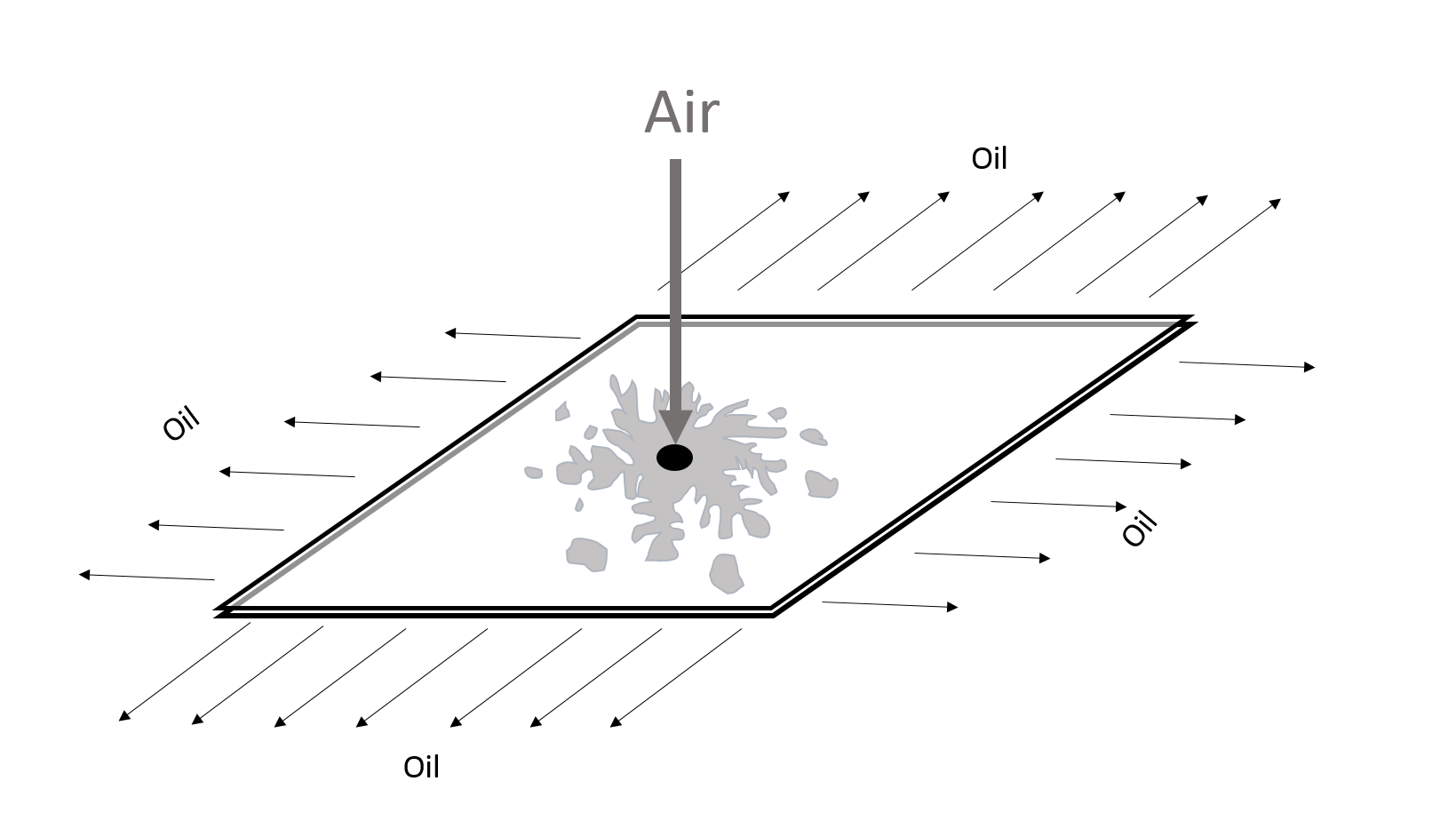
Figure 1: A low viscosity fluid, say air, is pumped through a hole (black circle) in one of the glass plates constricting the gap of the Hele-Shaw cell, which is otherwise filled with a high viscosity fluid, say oil. As air is pumped, oil escapes through the sides of the cell, while a droplet with an intricate interface is formed. Depending on the protocol of injection, the interface may become multi-connected.

The rate of injection is immaterial to the shapes that appear, and as such we may assume this rate to be constant. Since then the area inside the interface increases linearly, we may measure time in units of the area of the low viscosity droplet. We may thus henceforth talk of the phsycal time and the area of the low viscosity droplet interchangeably.

A theoretical prediction of the fractal dimension and other fractal properties of the cluster has long been at the focus of a fairly large body of scientific research (although interest may have waxed and waned). The purpose of the current article is twofold. First, we wish to review an approach to tackle the problem based on the relation of Hele-Shaw growth to classical integrability. Second, we wish to propose a tentative new direction of research based on quantum integrability.

As a definition of the fractal dimension of the interface we shall take use relation between the linear size of the droplet $R$ and the area of the low viscosity droplet $t$. We define the fractal dimension through the observed power law relation between the two:

$$R^{D}=t.$$ (1.1)

We leave open the question of how to define of the linear size of the droplet, $R$. In addition we shall assume that the relation (1.1) holds sharply, namely that $D$ defined above does not fluctuate.

1.2 The Hele-Shaw Probability Density

One of the main goals within the theory of the Hele-Shaw problem is to find the function giving the probability density to find Hele-Shaw interfaces of different shapes. Let us define $t(\mathcal{C})$ as the area inside the interface $\mathcal{C}$, and the probability distribution function , $P(\mathcal{C})$, as the probability density to find an interface $\mathcal{C}$ at time $t(\mathcal{C})$, given some probability distribution on the initial condition $P_{0}(\mathcal{C})$. Let $\mathcal{C}^{\Delta t}$ be the the interface $\mathcal{C}$ evolved a time $\Delta t$. Namely, if $\mathcal{C}$ has area $t$, then $\mathcal{C}^{\Delta t}$ has area $t+\Delta t$. The function $P$ is defined as follows:

$$P(\mathcal{C})=P_{0}(\mathcal{C}^{-t(\mathcal{C})})$$ (1.2)

We shall specify the measure $d\mathcal{C},$ with respect to which the probability density $P(\mathcal{C})$ is defined, but shall only demand that it is time translation invariant, $d\mathcal{C}=d\mathcal{C}^{\Delta t}$ . Indeed, Eq. (1.2) makes little sense otherwise.

The probability density $P$ is time translation invariant. Indeed, from (1.2) one may easily show

$$P(\mathcal{C}^{\Delta t})=P(\mathcal{C}).$$ (1.3)

The function $P$ possesses scale invariance, as well. Let us define, with some abuse of notations, $P(R)$ as follows:

$$P(R)=\int P(\mathcal{C})\delta(R-R(\mathcal{C}))d\mathcal{C},$$ (1.4)

where $R(\mathcal{C})$ is the linear size of the interface. For Laplacian growth we assume Eq. (1.1) holds which, we shall see, leads to:

$$P(R)dR=dR^{D}.$$ (1.5)

Indeed,

$$P(R)=\int P(\mathcal{C})\delta\left(R-t^{1/D}(\mathcal{C})\right){d\mathcal{C}}=$$ (1.6)

$$=DR^{D-1}\int P(\mathcal{C})\delta\left(R^{D}-t(\mathcal{C})\right)d\mathcal{C}=$$ (1.7)

$$=DR^{D-1},$$ (1.8)

where the last equality follows from the fact that the measure is time translation invariant.

We note that the time translation invariance of the probability density means that the probability measure can be thought as a probabilistic uniform superposition of the interface at different times. That the probability density is also scale invariant is a demonstration of the fractal property of the interface, namely Eq. (1.1), such the two properties together define the problem of finding the probability density which encodes the fractal dimensions.

A further important comment is that in searching for the probability density obeying scale and time translation invariance, the problem may be somewhat generalized in the following sense. The droplet in the Laplacian problem remains singly connected if the injection of the low viscosity fluid is always fast enough to rule out surface tension effects. However, if the protocol of injection is altered the droplet may become multi-connected. Imagine, for example taking a large droplet, with a fully-developed fractal structure over many scales. The interface is self similar in that if the low viscosity fluid is extracted, allowing the droplet to shrink, but we re-scale the resulting interface by a proper factor, one obtains the original droplet. Assume now that before extracting the low viscosity fluid we wait some time and allow surface tension to change the shape. This has the effect of coarsening the shape on the lowest scales as well as allowing for the possibility for the droplet to become multi-connected. Then some low viscosity fluid is quickly extracted. We may still expect that the self-similarity, though perhaps in a weaker sense, is preserved. It seems then that the single-connectedness of the droplet should not be imposed as a strict condition. As a result we consider probability densities which give non-zero measure to multi-connected droplets.

1.3 Preview of the Paper

The fact that the time translation invariance property of the probability distribution function, Eq. (1.3), coexists with the scale invariance property, Eq. (1.5), is equivalent to the scaling law $R^{D}(\mathcal{C})=t(\mathcal{C})$. We may formulate the problem of determining $D$, the fractal dimension, as finding the scaling law (1.5) for a probability distribution function obeying the time translation invariance property, Eq. (1.3). The current paper puts forward the proposition that candidates for the probability distribution function may be found within the realm of quantum integrable systems and conformal field theory .

Let us briefly recount the connection between fractal structures and conformal field theory. The context in which the two concepts may be most successfully linked is within the framework of equilibrium two dimensional critical phenomena. There, scale invariance, which is a consequence of the divergence of correlation lengths leads to conformal invariance, and it is assumed that, at the critical point, the statistical mechanics problem is described by conformal field theory. The vacuum is a Gibbs state in which fractal objects, such as cluster boundaries, exist at all length scales. A fractal cluster may then be pinned to a particular point by applying a scaling field at that point[5]. The dimension of the scaling field is determined by the power-law dependence of the scaling field on the small scale cut-off. Since this cut-off also determines the probability that the fractal can be found and pinned to a small box of linear size given by the cut-off scale, and this in turn is related to the notion of box-counting fractal dimension, there is a relation between the dimension of the scaling field and the fractal dimension of the object being pinned by it.

Non-equilibrium problems, such as Laplacian growth, are unlikely to be linked in the same manner to conformal field theory. Indeed, it does not seem a reasonable assumption that the Laplacian growth interface may be pinned to a point by applying, to some vacuum containing already many fractal structures on all scales, a scaling field of conformal field theory. Such a scenario would mean that the fully developed large area interface can be picked at once from a Gibbs state without a need to apply the nonlinear evolution from an initial interface. In other words, such a scenario would mean that there is a representation of the interface as an equilibrium object.

Nevertheless, a connection to conformal field theory is an appealing prospect, due to the fact that conformal field theory is inherently scale invariant, just as the fractal dimension of the interface is, and due to the fact that such a connection would alow for tools to predict the fractal dimensions, since conformal field theory naturally supplies a discrete spectrum of possible scaling dimensions, these in turn possibly determining the fractal dimension.

Here we propose that instead of basing the connection to conformal field theory on the notion of scale invariance being promoted to conformal invariance, a relation to conformal field theory may be established making use of the fact that conformal field theory has a hidden integrable structure, a structure which can be viewed as a quantization of the integrable structure hidden in Laplacian growth. At present, we are only able to make this connection within some limit, where only a small part of the interface, which happens to be long and narrow, is focused upon. Within this limit, the integrable structure of Laplacian growth becomes that of the Korteweg-de Vries equation, the quantum analogue of which is the integrable structure hidden within conformal field theory.

To flesh out this connection, we review first the integrable structure within Laplacian growth[6, 7, 8, 9] in section 2. This integrable structure turns out to be the dispersionless limit of a reduction of the two dimensional Toda lattice. Since we are eventually interested in the quantum integrable system, we must discuss how this dispersionless limit is obtained from a fully quantum system. To this end section 3 and 4 describe how the dispersionless limit is removed to obtain the full but reduced and classical two dimensional Toda lattice. The next logical step would be to pass to the quantum problem. However, before discussing how to quantize the problem, we pass, on a classical level, from the two dimensional Toda lattice to the Korteweg-de Vries equation[10]. This is done in section 5, and includes focusing on a long and narrow finger of the Laplacian growth. In section 6 we discuss the quantization of the problem[11, 12, 13, 14, 15], which leads us to the quantum Korteweg de-Vries equations. This quantum problem lies at the heart of conformal field theory. This fact allows us, in section 7, to show how a certain object, familiar within the framework of conformal and integrable field theory, may describe the classical Laplacian growth problem, through the probability distribution function $P(\mathcal{C})$. Section 8 contains concluding remarks.

2 Classical Integrability in Laplacian Growth

Here we review some of the mathematical structures underlying the problem of Laplacian growth. This includes the description through conformal maps and classical integrability[6, 7].

2.1 Description Through Conformal Maps

Let us consider the Hele-Shaw setup, which was already described in the introduction. The ambient, high viscosity fluid is described by a velocity field $\vec{v}$. This velocity is the average velocity across the gap between the two glass plates. Due to the high viscosity of the fluid, one must balance the internal viscous friction force experienced by the fluid, with the force supplied by the pressure, neglecting inertia, which is small because of the small separation of the plates. As the force of friction scale with the average velocity across the gap $\vec{v}$ , with the magnitude of the viscosity, $\mu$, and inversely with the size of the gap squared, $\frac{1}{b^{2}}$ one obtain Darcy’s law:

$$\frac{12\mu}{b^{2}}\vec{v}=-\vec{\nabla}P.$$ (2.1)

The factor $12$ may be obtained by a more detailed, but basic calculation, which takes into account the no-slip conditions at the interface between the fluid and the glass plates, which results in a parabolic velocity profile.

The dynamics are dictated by the following conditions. The motion of the interface between the inviscid and viscous fluid are determined by the normal velocity at the interface, which is proportional to the normal derivative of the pressure at the interface:

$$v_{n}=-\frac{b^{2}}{12\mu}\partial_{n}P.$$ (2.2)

Incompressibility, $\vec{\nabla}\cdot\vec{v}=0$, requires, that there exists a real stream function, $\varphi$:

$$\vec{v}=\frac{Q}{2\pi}\hat{z}\times\vec{\nabla}\theta,$$ (2.3)

where $\hat{z}$ is the out-of-plane unit vector and $Q$ is the volume flux, namely the volume of fluid injected into the cell in unit time, inserted here for convenience, as to make $\varphi$ dimensionless.

Defining the complex function $v$ by $v=v_{x}+\imath v_{y}$, and taking $\partial$, and $\bar{\partial}$ to be a derivative with respect to $z$ and $\bar{z}$, respectively ($\partial=\frac{\partial_{x}-\imath\partial y}{2},$ $\bar{\partial}=\frac{\partial_{x}+\imath\partial y}{2}$), we may write the relations between the pressure, the stream function and the velocity as:

$$v=-\frac{b^{2}}{6\mu}\bar{\partial}P=\frac{Q}{\pi}\imath\bar{\partial}\theta$$ (2.4)

We may define a complex analytic potential $\varphi_{t}$ (where in $\varphi_{t}$ the index denotes explicitly the time dependence):

$$\varphi_{t}(z)=\theta-\imath\frac{\pi b^{2}}{6Q\mu}P.$$ (2.5)

Indeed, relation (2.4) suggests that $\varphi_{t}(z)$ is analytic $\bar{\partial}\varphi_{t}=0,$ Taking the complex conjugate of (2.4) also leads, after simple algebra, to:

$$\bar{v}=-\frac{\imath Q}{2\pi}\partial\varphi_{t}.$$ (2.6)

The pressure is constant inside the droplets of lower viscosity, since the fluid there has neither inertia (due to the narrowness of the gap) nor viscosity (by assumption). We may assume this pressure to be zero. This means that we assume a type of dynamics in which, even after the low viscosity droplet breaks up into several droplets, the same pressure is maintained across the different droplets. This scenario cannot be attained in a Hele-Shaw cell, since only one of the droplets will be connected to the source of low viscosity fluid through the hole. One may imagine instead of a glass plate using a plate made of a material permeable to the low viscosity fluid but impregnable to the high viscosity fluid. The low viscosity fluid may then be supplied through the entire plate, and the different droplets will maintain the same pressure, which without loss of generality may be set to zero, since only gradients of the pressure play any role in the dynamics.

We now consider the analytic properties of $\varphi_{t}$. First note that we assume that the fluid is syphoned off in a radially symmetric fashion around infinity, which suggests $v(r)\sim\frac{Q\hat{r}}{2\pi r}$ as $r\to\infty$. This leads to the following asymptotic behavior of $\varphi_{t}:$

$$\varphi_{t}(z)\sim-\imath\log(z),\quad\mbox{as }z\to\infty,$$ (2.7)

which leads to the fact that the imaginary part of $\varphi+t$, namely the stream function $\varphi$ winds by $2\pi$ as one encircles infinity. In fact $\varphi_{t}$ is only well-defined if a branch cuts are introduced in the complex plane, such that from each droplet a branch cut extends to infinity. This can be understood by considering that the winding by $2\pi$ of $\varphi_{t}$ around infinity has its origin in the winding of $\theta$ around the droplets. Indeed, consider the integral over the velocity around the droplet. From simple hydrodynamical kinematics, this integral is equal to volume flux of fluid entering the cell, on the one hand, and from the definition of the stream function, Eq. (2.3), it is equal to the integral over the gradient of $\theta$ around the droplets:

$$Q=\oint\vec{v}\times d\vec{r}=\frac{Q}{2\pi}\oint\vec{\nabla}\theta\cdot d\vec{r},$$ (2.8)

leading to the conclusion that the winding of $\varphi$ around the droplets is $2\pi$:

$$\oint\vec{\nabla}\theta=2\pi.$$ (2.9)

The the variable $\theta$ can thus be used as a coordinate along the droplets, whose range is $[0,2\pi]$.

A central role will be given to the inverse function of $\imath\varphi_{t}$, which we shall denote by $f_{t}$:

$$f_{t}(\imath\varphi_{t}(z))=z$$ (2.10)

$f_{t}(\imath\varphi)$ is defined such that for $\varphi\in[0,2\pi]$, the function $f_{t}(\imath\varphi)$ gives the complex coordinate of a point on the interface of the droplets, with given $\theta$ and at time $t$. The function $f_{t}$ is defined with period $\imath 2\pi$:

$$f_{t}(\imath\varphi+2\pi\imath)=f_{t}(\imath\varphi),$$ (2.11)

For complex $\varphi$, the function $f_{t}(\imath\varphi)$ is defined by analytic continuation. As a result of the periodicity, the function $f_{t}$ is defined on a cylinder, $\mathcal{S}$, where points displaced by $2\pi\imath$ are identified, $\mathcal{S}=\mathds{C}/2\pi\imath\mathds{Z}$. The function $f_{t}(\imath\varphi)$ has the following expansion at ${\rm Im}(\varphi)\to-\infty:$

$$f_{t}(\imath\varphi)=a_{1}^{(1)}e^{\imath\varphi}+a_{0}^{(1)}+a_{-1}^{(1)}e^{-\imath\varphi}+\dots=\sum_{j=-1}^{\infty}a^{(1)}_{-j}e^{-\imath j\varphi},$$ (2.12)

which results from (2.7).

Since the interface is described by the map $f_{t}(\imath\varphi):[0,2\pi]\to z$ and since $f_{t}$ is periodic in $2\pi\imath$, there is an arbitrariness in choosing $f_{t}(\imath\varphi)$ given the shape of the interface. Indeed the functions $f_{t}(\imath\varphi)$ and $f_{t}(\imath(\varphi+c))$ describe the same interface, the only difference being that the reference point on the interface where the angle $\theta$ is considered as $0$ is moved from $f_{t}(0)$ to $f_{t}(\imath c)$. Thus, when describing the dynamics of the interface as the dynamics of $f_{t}$, one has to bear in mind that the dynamics of $f_{t}$ which are equivalent to shifting the reference point of $\varphi$ are meaningless and arbitrary. It is common in the literature to remove this arbitrariness by requiring $a_{1}^{(1)}$ to be real. We shall not follow that convention, and rather leave this arbitrariness in place.

An useful mathematical object to study interfaces in two dimensions is is the Schwarz function, $S(z)$ – the an analytic continuation of a function giving $\bar{z}$ on the boundary. Namely for $z\in\mathcal{C}$, we have $S(z)=\bar{z}$, with $S(z)$ being analytic in a neighborhood of $\mathcal{C}$. One may easily ascertain that the Schwarz function can be written as

$$S(z)=\bar{f}_{t}(-\imath\varphi_{t}(z)),$$ (2.13)

where, as usual, for any function $g(z)$, the function $\bar{g}(z)$ is defined as $\overline{g(\bar{z})}$. To see that (2.13) indeed gives the Schwarz function, consider that for $z$ on the boundary, $\varphi_{t}(z)$ , is purely real and so, $\bar{f}_{t}(-\imath\varphi_{t}(z))=\overline{f_{t}(\imath\varphi_{t}(z))}=\bar{z}.$ The Schwarz function, $S(z),$ obeys the ‘unitarity’ condition:

$$\bar{S}(S(z))=z.$$ (2.14)

This relation is proven by considering it on the interface, where it simply follows from the fact that $S(z)=\bar{z}$ on the interface, and then trivially analytically continuing the relation away from the interface.

2.2 Richardson Moments

As was found by Richardson [9], during the course of the evolution an infinite set of parameters, namely the Richardson moments remain constant. The $k$’th Richardson moment is defined as:

$$t_{k}=\int_{\mathcal{D}_{+}}\frac{dz\wedge d\bar{z}}{2\pi\imath kz^{k}},$$ (2.15)

where $\mathcal{D}_{+}$ denotes the domain which is exterior to the droplet. To see that these are conserved consider $\dot{t}_{k}$:

$$\dot{t}_{k}=\hat{z}\cdot\oint_{\mathcal{C}}\frac{d\vec{r}\times\vec{v}}{2\pi\imath kz^{k}}.$$ (2.16)

We may write $\hat{z}\cdot d\vec{r}\times\vec{v}=\frac{\imath}{2}(dz\bar{v}-d\bar{z}v)$. We may re-write the right hand side of this equation using (2.6) as $\frac{Q}{4\pi}(dz\partial\varphi+d\bar{z}\bar{\partial}\varphi)=\frac{Q}{4\pi}d\varphi_{t}$, one obtains:

$$\dot{t}_{k}=\frac{Q}{8\imath\pi^{2}k}\oint\frac{d\varphi_{t}}{z^{k}},$$ (2.17)

As the integrand is analytic in $\varphi_{t}$, the contour of integration may be deformed to a large contour surrounding infinity in the $z$-plane, where the asymptotic relation $\varphi_{t}\sim-\imath\log z$ holds. This yields:

$$\dot{t}_{k}=\frac{Q}{8\imath\pi^{2}k}\oint_{\infty}\frac{dz}{z^{k+1}}=0.$$ (2.18)

Note also that the Schwarz function encodes the harmonic moments. Indeed, Stokes theorem states that (2.15) can be written as a contour integral over the boundary of the droplets $t_{l}=\oint_{\mathcal{C}}\bar{z}z^{-l}\frac{dz}{2\pi\imath l}$ and since one the contour $S(z)=\bar{z}$, this can be written as:

$$t_{l}=\oint S(z)z^{-l}\frac{dz}{2\pi\imath l},\quad t=\oint S(z)\frac{dz}{2\pi\imath}.$$ (2.19)

One may construct from knowledge of the Richardson moments, $t_{k}$, and the area of the droplets, $t$ its shape, given some additional data, such as the number of connected components. The Richardson moments are thus reminiscent of the conserved quantities of completely integrable systems, since the knowledge of which is enough to determine completely the dynamics. The results of Refrs. [6, 7, 8] show, however, that the actual integrable structure behind the zero surface-tension Hele-Shaw problem treats the Richardson moments rather as the ‘times’ conjugate to the conserved quantities, or ‘Hamiltonians’, which may be denoted by $H_{k}$. In addition it is appropriate to treat the complex conjugate of the Richardson moments (which are themselves complex quantities), namely the quantities $\bar{t}_{k}$, as additional independent times, with which one associated a set of Hamiltonians, $\bar{H}_{k}$.

To be able to define the Hamiltonians, $H_{k}$, $\bar{H}_{k}$, we must first define a Poisson bracket. This is given by:

$$\{\imath\varphi,t\}=1.$$ (2.20)

With this definition of the Poisson bracket, the evolution of $f_{t}$ is encoded in the following relations:

$$\{f_{t}(\imath\varphi),\bar{f}_{t}(-\imath\varphi)\}=1,$$ (2.21)

which, due to $\bar{f}_{t}(-\imath\varphi)=S(f_{t}(\imath\varphi)),$ can also be written as:

$$\{f_{t}(\imath\varphi),S(f_{t}(\imath\varphi))\}=1.$$ (2.22)

That the evolution of $f_{t}$ is determined by (2.21) can be shown as follows. First note that (2.21) can be written as:

$${\rm Im}\partial_{t}f_{t}\partial_{\varphi}\bar{f}_{t}=1.$$ (2.23)

Since $\partial_{t}f_{t}$ is the velocity of a point on the interface with given $\varphi$, we may write it in usual vector notation as $\vec{\tilde{v}}$, the tilde denoting that it may not be equal to the velocity of the fluid. Nevertheless, its normal component must be equal to the velocity of the fluid so we have $\tilde{v}_{n}=v_{n}$. Furthermore, $\partial_{\varphi}f_{t}$ may be written in vector notations as $\frac{d\vec{r}}{d\varphi}$. Taking into account that if $a=a_{x}+\imath a_{y}$ and $b=b_{x}+\imath b_{y}$ are the complex notations for $\vec{a}$ and $\vec{b}$, then the vector product is given by $\vec{a}\times\vec{b}=\hat{z}{\rm Im}(a\bar{b})$, we may rewrite (2.23) as:

$$\vec{\tilde{v}}\times\frac{d\vec{r}}{d\varphi}=1.$$ (2.24)

This relation implies $v_{n}\frac{dl}{d\varphi}=1$, or $v_{n}=\frac{d\theta}{dl}.$ Now, since $\theta$ and $\frac{\pi b^{2}}{6Q\mu}P$ are conjugate harmonic functions (Eq. (2.5)), one may use the Cauchy-Riemann relations to obtain $\frac{d\varphi}{dl}=-\frac{b^{2}}{6Q\mu}\frac{dP}{dn}$, yielding the equation governing the evolution of the droplet, Eq. (2.2).

The evolution with respect to the physical time, is given by relation (2.21). Alternatively, we can write:

$$\partial_{t}f=\{\imath\varphi,f\},$$ (2.25)

showing that the designation of the Hamiltonian that generate the time translations as $\imath\varphi$ is appropriate. We may thus write $H=\imath\varphi$. Note however, that Eq. (2.25) is almost an empty statement, in the sense that the evolution of $f$ cannot be extracted from it, as the right hand side is identically equal to the left hand side irrespective of the time evolution of the droplet.

Another way to describe the evolution is through the Schwarz function. Writing the Poisson bracket in (2.22) explicitly and dividing by $\frac{\partial f_{t}}{\partial\varphi}$, one obtains:

$$\frac{\partial S(f_{t}(\imath\varphi))}{\partial t}=\frac{1}{\frac{\partial f_{t}(\imath\varphi))}{\partial\varphi}}\left(\imath+\frac{\partial f_{t}(\imath\varphi)}{\partial t}\frac{\partial S(f_{t}(\imath\varphi))}{\partial\varphi}\right).$$ (2.26)

Evaluating this equation at $\varphi=\varphi_{t}(z)$ and making use of

$$\left.\frac{\partial f_{t}(\imath\varphi))}{\partial\varphi}\right|_{\varphi=\varphi_{t}(z)}=\left(\frac{\partial\varphi_{t}(z)}{\partial z}\right)^{-1}\mbox{ and}\quad\frac{\partial\varphi_{t}(z)}{\partial t}\frac{\partial f_{t}(\imath\varphi)}{\partial\varphi}+\left.\frac{\partial f_{t}(\imath\varphi)}{\partial t}\right|_{\varphi=\varphi_{t}(z)}=0,$$ (2.27)

yields:

$$\frac{\imath\partial\varphi_{t}(z)}{\partial z}=\frac{\partial\varphi_{t}(z)}{\partial t}\frac{\partial S(f_{t}(\imath\varphi))}{\partial\varphi}+\left.\frac{\partial S(f_{t}(\imath\varphi))}{\partial t}\right|_{\varphi=\varphi_{t}(z)}.$$ (2.28)

The right hand side can be identified with $\frac{\partial S(z)}{\partial t}$ such that we have:

$$\frac{\partial S(z)}{\partial t}=\frac{\imath\partial\varphi_{t}(z)}{\partial z},$$ (2.29)

which constitutes a simple evolution equation for the Schwarz function.

Eq. (2.29) is useful to show that the dynamics prescribed by (2.21) is such that the pressure is equal on all interfaces. This needs to be shown because above we have only assumed that the pressure is constant on any connected component of the interface. Suppose then that points $a$ and $b$ are on the interface, perhaps on different connected components of which. Eq. (2.29) together with (2.5) allows us to write:

$$\frac{P(a)-P(b)}{\frac{\pi b^{2}}{6Q\mu}}={\rm Re}\frac{\partial}{\partial t}\int_{a}^{b}S(z)dz.$$ (2.30)

On the other hand we have:

$$\int_{a}^{b}S(z)dz=-\overline{\int_{\overline{S(a)}}^{\overline{S(b)}}S(y)dy}+\left.zS(z)\right|^{b}_{a},$$ (2.31)

which is obtained by first changing the integration variable from $z$ to $y=\overline{S(z)}$, on the left hand side, this change of variables being facilitated by using unitarity, Eq. (2.14), to obtain $z=\overline{S(y)}$, then integrating by parts the result. Taking the real part of Eq. (2.31) and a time derivative, one obtains:

$$2{\rm Re}\int_{a}^{b}\partial_{t}S(z)dz={\rm Re}\left(z\partial_{t}S(z)-\bar{z}\partial_{t}\overline{S(z)}\right)=0,$$ (2.32)

which when compared to (2.30) yields:

$$P(a)=P(b),$$ (2.33)

for any two points $a$, $b$ on the interface, including points on different connected components.

2.3 Integrability of Laplacian growth

Integrability of Laplacian growth is the statement that the evolution of the Hele-Shaw interface can be described by a Hamiltonian, $H$, which is in involution with an infinite set of other Hamiltonians (conserved quantities) , $H_{k},$ with respect to some Poisson bracket. As usual, the other Hamiltonians, in Laplacian growth can be used to generate flows with respect to new times $t_{k},$ in one to one correspondence to the Hamiltonians, $H_{k}$. These Hamiltonians in Laplacian growth can be chosen such that $t_{k}$ are the Richardson moments of the interface. Namely, the Hamiltonians, $H_{k},$ generate deformations of the interface corresponding to changing the Richardson moments $t_{k}$, respectively. Due to the fact that these moments are complex, the Hamiltonians are also complex and to each $H_{k}$ we may associate a $\bar{H}_{k}$, which generates, formally, deformations which correspond to changing $\bar{t}_{k}$. Of course one cannot change $t_{k}$ without changing $\bar{t}_{k}$, yet, as usual, they may be treated as independent variables, just as $H_{k}$ and $\bar{H}_{k}$ may be treated as independent conserved quantities or Hamiltonians.

The Hamiltonians read explicitly:

$$H_{k}(\varphi,t)=\left({f_{t}^{k}(\imath\varphi)}\right)_{+}+c^{(k)},$$ (2.34)

where $c^{(k)}$ is a an arbitrary function of the times only, which (as shall be seen below) does not affect the dynamics, while the index $+$ denotes taking the positive (polynomial) part of the Laurent expansion around infinity in the variable $e^{\imath\varphi}$, using the following convention. Due to Eq. (2.12) we may expand $f^{k}_{t}$ as

$$f_{t}^{k}=\sum_{j=-\infty}^{k}a_{j}^{(k)}e^{\imath j\varphi}.$$ (2.35)

The positive part of this series is defined as follows:

$$\left({f_{t}^{k}(\imath\varphi)}\right)_{+}=\frac{a^{(k)}_{0}}{2}+\sum_{j=1}^{k}a_{j}^{(k)}e^{\imath j\varphi},$$ (2.36)

which is natural, except the zeroth order term, defined with a factor $1/2$ for later convenience.

The Hamiltonian $\bar{H}_{k}$ is defined as follows:

$$\bar{H}_{k}(\varphi,t)=\overline{H_{k}(\bar{\varphi},t)}=\left({\bar{f}_{t}^{k}(-\imath\varphi)}\right)_{+}+\bar{c}^{(k)}.$$ (2.37)

We now show that the evolution generated by the Hamiltonians,

$$\frac{\partial f_{t}(\imath\varphi)}{\partial t_{k}}=\{f_{t}(\imath\varphi),H_{k}\},$$ (2.38)

$$\frac{\partial f_{t}(\imath\varphi)}{\partial\bar{t}_{k}}=-\{f_{t}(\imath\varphi),\bar{H}_{k}\},$$ (2.39)

effect a deformation of the contour corresponding to changing the Richardson moments. Namely, we show that if (2.15) holds at any moment in times, then it holds for all subsequent times, for the evolution prescribed by (2.38), (2.39).

First note that the complex conjugate of Eq. (2.39) can be also cast as the evolution of the Schwarz function. Indeed, the complex equation of that equation, has the following form:

$$\frac{\partial\bar{f}_{t}(-\imath\varphi)}{\partial t_{k}}=\{\bar{f}_{t}(-\imath\varphi),H_{k}\},$$ (2.40)

which is the evolution of the Schwarz function, $S(z)=\bar{f}_{t}(-\imath\varphi_{t}(z))$, evaluated at $z=f_{t}(\varphi)$. We proceed by first showing:

$$\frac{\partial S(z)}{\partial t_{k}}=\frac{\partial H_{k}}{\partial z},\quad\frac{\partial S(z)}{\partial\bar{t}_{k}}=\frac{\partial\bar{H}_{k}}{\partial z}.$$ (2.41)

We do this by writing:

$$\frac{\partial S(z)}{\partial t_{k}}=\frac{\partial\bar{f}_{t}(-\imath\varphi)}{\partial t_{k}}+\left.\frac{\partial\varphi_{t}(z)}{\partial t_{k}}\frac{\partial\bar{f}_{t}(-\imath\varphi)}{\partial\varphi}\right|_{\varphi=\varphi_{t}(z)}$$ (2.42)

Using (2.38) and the first equation in (2.27) along with

$$\frac{\partial\varphi_{t}(z)}{\partial t_{k}}=-\left.\frac{\partial f_{t}(\imath\varphi)}{\partial t_{k}}\left(\frac{\partial f_{t}(\imath\varphi)}{\partial\varphi}\right)^{-1}\right|_{\varphi=\varphi_{t}(z)},$$

one may re-write (2.42) as:

$$\frac{\partial S(z)}{\partial t_{k}}=\frac{\partial H_{k}}{\partial\varphi}\left.\left(\frac{\partial S(f_{t}(\imath\varphi))}{\partial t}+\frac{\partial S(z)}{\partial z}\frac{\partial f_{t}(\imath\varphi)}{\partial t}\right)\right|_{\varphi=\varphi_{t}(z)}=\frac{\partial S(z)}{\partial t}\left.\frac{\partial H_{k}}{\partial\varphi}\right|_{\varphi=\varphi_{t}(z)}.$$ (2.43)

Making use now of (2.29) , the first equation in (2.41) follows. The second equation in (2.41) may be derived by the analogous manipulations.

Given (2.41), and the definition of $H_{k}$, we may write

$$\frac{\partial S(z)}{\partial t_{k}}=kz^{k-1}+O(1/z^{2}),\quad\frac{\partial S(z)}{\partial\bar{t}_{k}}=O(1/z^{2}).$$ (2.44)

Indeed, substituting into the first equation in (2.41) the explicit expression for $H_{k}$ and evaluating at $\varphi=\varphi_{t}(z)$, leads to the first equation. For the second equation note that $\bar{H}_{k}$ contains only negative powers of $e^{\imath\varphi}$. These, in turn, when evaluated at $\varphi=\varphi_{t}(z)$ can be written as negative powers of $z$, due to (2.12), leading to the second equation in (2.44). Equation (2.44) immediately implies:

$$\oint_{\mathcal{C}}z^{-l}\frac{\partial S(z)}{\partial t_{k}}\frac{dz}{2\pi\imath k}=\delta_{kl},\quad\oint_{\mathcal{C}}z^{-l}\frac{\partial S(z)}{\partial\bar{t}_{k}}\frac{dz}{2\pi\imath k}=0.$$ (2.45)

Taking a derivative with respect to $t_{k}$ and $\bar{t}_{k}$ of Eq. (2.19), one realizes that Eq. (2.45) is just the differential form of these equations. Thus we have proven the required statement.

Note that $c^{(k)}$ in (2.34) are indeed arbitrary, in the sense that we did not need to assume anything about them to prove that (2.19) follow from (2.38), (2.39). In fact, $c^{(k)}$ just generates transformations that shift the reference point for the angle $\varphi$. To see this consider that one always applies the Hamiltonians in a real combination. Namely any deformation of the droplet is effected by:

$$\delta f_{t}=\sum_{k}\{f_{t},\delta t_{k}H_{k}-\delta\bar{t}_{k}\bar{H}_{k}\}.$$ (2.46)

The free ($\varphi$-independent) term in $\delta t_{k}H_{k}-\delta\bar{t}_{k}H_{k}$ reads $2\imath{\rm Im}(\delta t_{k}c^{(k)})$, while the latter generates the following deformation of $f_{t}$:

$$\{f_{t},2\imath{\rm Im}(\delta t_{k}c^{(k)})\}=2{\rm Im}(\delta t_{k}\dot{c}^{(k)})\frac{\partial f_{t}}{\partial\varphi},$$ (2.47)

where the dot signifies a $t$ derivative. Thus, $2\imath{\rm Im}(\delta t_{k}c^{(k)})$ indeed is the generator of real, times-dependent $\varphi$ translations, and thus do not deform the interface. As a result, we may choose $c^{(k)}$ freely.

We make the choice of $c^{(k)}$ such that it is consistent with the involution of the Hamiltonians. Consider first the indefinite integral $\int S(z)dz=\sum_{k}t_{k}z^{k}+t\log(z)+c+O(1/z),$ where $c$ is an arbitrary function of the times, the arbitrariness of $c$ being due to the indefiniteness of the integral. We may choose $c$ such that $\partial_{t}c=-\log(a_{0}^{(1)}),$ and define the result, which is now definite up to a time and $z$ independent additive factor as the integral of $S(z)$ :

$$\int S(z)dz=\sum_{k}t_{k}z^{k}+t\log(z)-\int_{0}^{t}\log(a_{0}^{(1)})+O(1/z).$$ (2.48)

The integral over $S$ is a generating function for the Hamiltonians. Indeed due to (2.41), we have:

$$\left.\frac{\partial}{\partial t_{k}}\int S(z)dz\right|_{z}=\alpha^{(k)}+H_{k},$$ (2.49)

for some $z$-independent constant, $\alpha^{(k)}$. We may choose $c^{(k)}$ such that this constant is zero, and write:

$$\left.\frac{\partial}{\partial t_{k}}\int S(z)dz\right|_{z}=H_{k},\quad\left.\frac{\partial}{\partial t}\int S(z)dz\right|_{z}=H.$$ (2.50)

This last equation (which is derived from the choice of $c^{(k)}$) states that $\int S(z)dz$ is a generating function for the Hamiltonians and, as shall be seen below, insures that the Hamiltonians are in involution. Indeed, The identities $\frac{\partial^{2}}{\partial t_{k}\partial t_{l}}=\frac{\partial^{2}}{\partial t_{l}\partial t_{k}}$, $\frac{\partial^{2}}{\partial t_{k}\partial\bar{t}_{l}}=\frac{\partial^{2}}{\partial\bar{t}_{l}\partial t_{k}}$, leads to:

$$\left.\frac{\partial H_{k}}{\partial t_{l}}\right|_{z}=\left.\frac{\partial H_{l}}{\partial t_{k}}\right|_{z},\left.\frac{\partial H_{k}}{\partial\bar{t}_{l}}\right|_{z}=\left.\frac{\partial\bar{H}_{l}}{\partial t_{k}}\right|_{z}\quad$$ (2.51)

and this yields the involution of the Hamiltonians, when written in terms of derivatives at fixed $\varphi$ rather than at fixed $z$; We first write:

$$\left.\frac{\partial H_{k}}{\partial t_{l}}\right|_{z}=\frac{\partial H_{k}}{\partial t_{l}}+\frac{\partial\varphi_{t}(z)}{\partial t_{l}}\left.\frac{\partial H_{k}}{\partial\varphi}\right|_{\varphi=\varphi_{t}(z)}=$$ (2.52)

$$=\frac{\partial H_{k}}{\partial t_{l}}-\left.\frac{\partial f_{t}(\imath\varphi)}{\partial t_{l}}\left(\frac{\partial f_{t}(\imath\varphi)}{\partial\varphi}\right)^{-1}\frac{\partial H_{k}}{\partial\varphi}\right|_{\varphi=\varphi_{t}(z)},$$ (2.53)

then subtract the equation with $k$ and $l$ interchanged and use (2.38) to obtain:

$$\frac{\partial H_{k}}{\partial t_{l}}-\frac{\partial H_{l}}{\partial t_{k}}-\{H_{k},H_{l}\}=0.$$ (2.54)

The latter being the required statement of the Hamiltonians being in involution. Of course one may easily obtain the following as well:

$$\frac{\partial H_{k}}{\partial\bar{t}_{l}}-\frac{\partial\bar{H}_{l}}{\partial t_{k}}-\{H_{k},\bar{H}_{l}\}=0.$$ (2.55)

3 Algebraic Solutions to Laplacian Growth

The interface may be described as a curve, namely as a relation between $x$ and $y,$ the Cartesian coordinates on the interface. This may be done by finding some function $\tilde{F}(x,y)$ such that $\tilde{F}(x,y)=0$ gives the interface. The ellipse is the simplest example except the circle. For the ellipse we have $\tilde{F}(x,y)=\frac{x^{2}}{r_{1}^{2}}+\frac{y^{2}}{r_{2}^{2}}-1$. Using complex coordinates one may alternatively describe the curve by a relation between $z$ and $\bar{z}$, for example, the ellipse may be described by $F(z,\bar{z})=\tilde{F}\left(\frac{z+\bar{z}}{2},\frac{z-\bar{z}}{2\imath}\right)=0,$ where $F(z,\bar{z})=\frac{1}{2}\left(\frac{1}{r_{1}^{2}}+\frac{1}{r_{2}^{2}}\right)|z|^{2}+\frac{1}{2}\left(\frac{1}{r_{1}^{2}}-\frac{1}{r_{2}^{2}}\right)(z^{2}+\bar{z}^{2}).$ One may solve this equation for $\bar{z}$. This gives the Schwarz function, $S(z)$, which satisfies $F(z,S(z))=0.$ If, as is true for the ellipse, the function $F(z,\bar{z})$ is a polynomial in both arguments, then $S(z),$ as a function of $z,$ is an algebraic function. As an example, for the ellipse we obtain:

$$S(z)=\frac{(r_{1}^{2}+r_{2}^{2})z+2r_{1}r_{2}\sqrt{z^{2}+r_{2}^{2}-r_{1}^{2}}}{r_{1}^{2}-r_{2}^{2}}.$$ (3.1)

Namely $S(z)$ contains roots and polynomials. As an algebraic function, $S(z)$ may be defined on a algebraic Riemann surface.

Defining the Schwarz function on the Riemann surface arises due to the fact that $S(z)$ is generically a multi-valued function, such as the function in (3.1), where the square roots makes $S(z)$ multi-valued. One is lead to resolve this multi-valuedness, by considering $m$ copies of the complex plane, one copy for each possible value of $S(z)$ for given $z$. Let us denote the $m$ possible values of $S(z)$ by $S^{(i)}(z),$ with $i=1,\dots,m$. Each copy of the complex plane must also be provided with branch cuts, in order to fully resolve the ambiguity. One should imagine cutting the sheets along the branch cuts. After cutting the sheet, each branch cut has the topology of a closed curve. On copy $i$ of the complex plane, the Schwarz function is designated the value $S^{(i)}(z)$ for given $z$. Then the different copies of the complex plane are glued together along the branch cuts, corresponding to the fact that as $z$ crosses the branch cut on sheet $i$ the function $S^{(i)}(z)$ will coincide smoothly with the value of function $S(z)$ on some other sheet, $j$.

For the example of the ellipse there are two sheets and

$$S^{(1,2)}(z)=\frac{(r_{1}^{2}+r_{2}^{2})z\pm 2r_{1}r_{2}\sqrt{z^{2}+r_{2}^{2}-r_{1}^{2}}}{r_{1}^{2}-r_{2}^{2}}.$$ (3.2)

The square root is taken in a way dictated by convention $\sqrt{re^{\imath\theta}}=\sqrt{r}e^{\imath\theta/2},$ for $-\pi\leq\theta<\pi.$ A branch cuts are drawn on both sheets between $\sqrt{r_{1}^{2}-r_{2}^{2}}$ (assuming $r_{1}>r_{2}$). And the two sheets are glued along the branch cut, the upper bank of the branch cut on first sheet to the lower bank of the branch cut on the lower sheet.

The algebraic Riemann surface, $\mathcal{A,}$ that is produced by considering the complex curve $F(z,S(z))=0$, is also called an algebraic curve[16] . It is composed of $m$ copies of the complex plane $\mathds{C}^{(i)}$ called sheets equipped with branch cuts. On each sheet, away from the branch cuts, one defines a holomorphic local parameter given by $z$. On the branch cuts, but away from the branch points, the local parameter spans more than one sheet. If $z_{0}$ is a simple branch point on sheet $i$, then the local parameter around the point is $\sqrt{z-z_{0}}$, spanning the two sheets that are connected at the branch point.

We may define a function on the algebraic curve $\mathcal{A}$ by specifying its values for any $z$ and any sheet $i$. It is thus convenient to introduce the notation $\bm{z}$ for a point on the $\mathcal{A}$, where $\bm{z}=\{z,i\}$, specifying the complex coordinate, $z$, of the point, and the sheet, $i$. For example, $S(\bm{z})$ is naturally defined as:

$$S(\bm{z})=S(\{z,i\})=S^{(i)}(z).$$ (3.3)

Finally, note that we shall called first sheet, $i=1$, also the ’upper sheet’, and all other sheets, collectively as ’lower sheets’.

The anti-analytic function $\tau(z)$, defined as:

$$\tau(z)=\overline{S(z)},$$ (3.4)

is, in fact, a one-to-one and onto map from the Riemann surface to itself. This is due to the fact that it is its own inverse $\tau(\tau(z))=z$, which is a consequence of unitarity (Eq. (2.14)). The set of points invariant with respect to $\tau$ is the interface of the droplet, $\tau(z)=z\Leftrightarrow S(z)=\bar{z}$. The anti-holomorphic involution, $\tau$, allows us to equivalently describe the Riemann surface as a Schottky double[17].

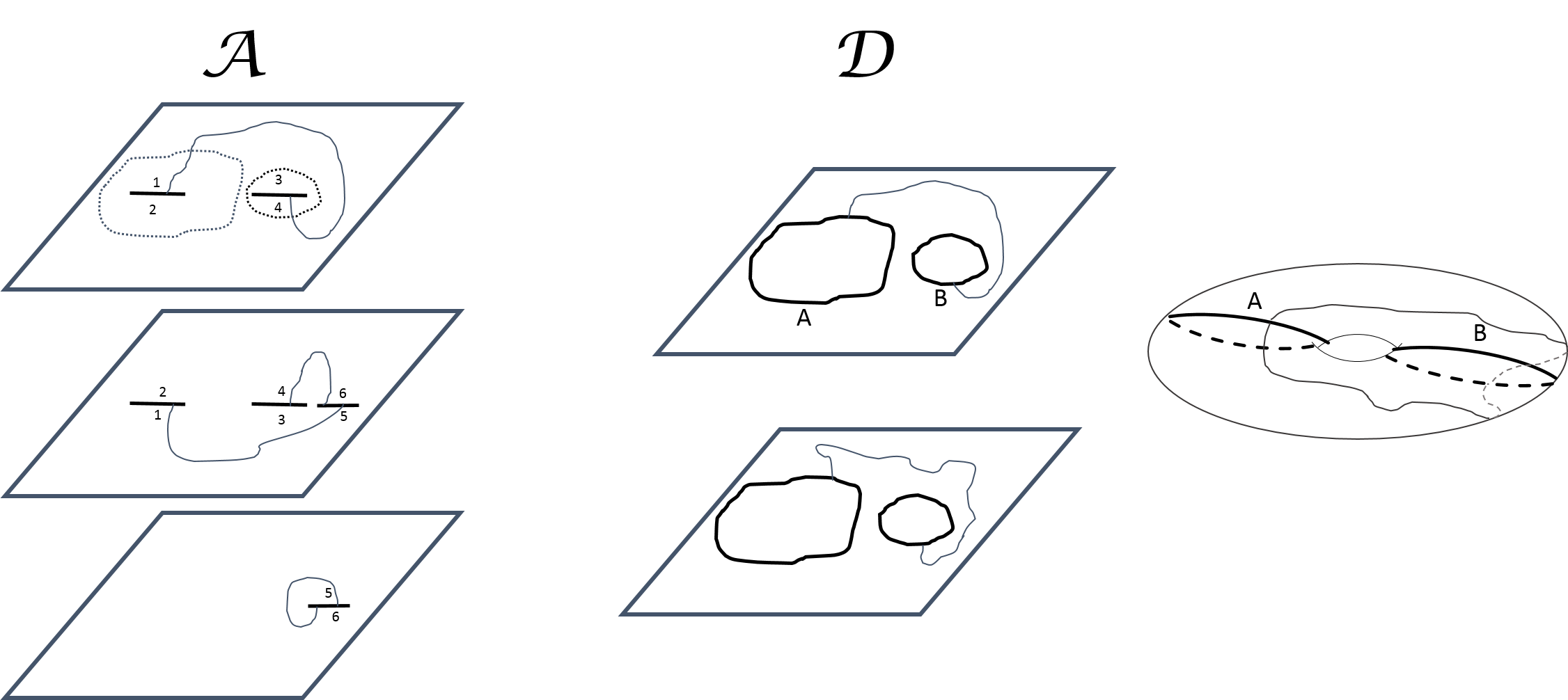
Figure 2: The construction of the Riemann surface as an algebraic curve, $\mathcal{A,}$ is drawn on the left. The surface is three sheeted. The two banks of each of the branch cuts are numbered, such that banks that are glued together on different sheets are given the same number. A meandering closed path, through the Riemann surface is also drawn. The dotted line is the interface. The algebraic curve $\mathcal{A}$ is mapped onto the Schottky double $\mathcal{D}$, in the middle drawing. The map of the meandering line is also drawn. The two connected components of the interface are now labelled $A$ and $B$. On the right is a torus of genus $1$ drawn as a doughnut. The interface with its two connected components, $A$ and $B,$ are drawn there, along with the meandering path. The torus is topologically equivalent both to the algebraic Riemann surface, $\mathcal{A}$ and the Schottky double $\mathcal{D}$.

To describe the Schottky double, consider two copies of that part of the complex plane that lies outside the droplet. Let us denote these two copies by $D^{(\uparrow)}$ and $D^{(\downarrow)}$, respectively. The Schottky double, $\mathcal{D}$ is defined to consist of the two copies of the exterior of the droplet, $D^{(i)}$, with local holomorphic coordinates inherited from the algebraic curve $\mathcal{A},$ through a one to one mapping $v,$ defined below, from the algebraic curve $\mathcal{A}$ to the Schottky double $\mathcal{D}$. The mapping $v$ is defined as follows:

$$v(\{z,i\})=\left\{\begin{array}[]{lr}\{z,\uparrow\}&\mbox{$i=1$ and $z$ outside $\mathcal{C}$}\\ \{\tau(z),\downarrow\}&\mbox{otherwise}\end{array}\right.$$ (3.7)

The upper sheet of the Schottky double, $D^{(\uparrow)}$ is usually called ‘the front side’, while the lower sheet, $D^{(\downarrow)},$ is commonly known, apparently, as ‘the back side’.

Note that since $\tau(z)$ is anti-holomorphic, the holomorphic coordinate on $D^{(\downarrow)}$ is $\bar{z}$, rather than $z$. Thus, by definition, an analytic on the Schottky double, is an analytic function of the variable $z$ on $D^{(\uparrow)}$ and an analytic function of the variable $\bar{z}$ on $D^{(\downarrow)}$. The function must also be analytic across the interface. Another way to describe an analytic function, $f$, on the Schottky doubleis to say that $f$ is analytic on the Schottky double, $\mathcal{D}$, if $g=f\circ\ v$ is analytic on the algebraic curve, $\mathcal{A}$.

As examples of analytic functions on the Schottky double, consider the function $id(\bm{z})$ defined as $id(\{z,\uparrow\})=z$, $id(\{z,\downarrow\})=\bar{z}$ . Another example (with some abuse of notations) is the function $S(\bm{z})$, defined as $S(\{z,\uparrow\})=S(z)$ and $S(\{z,\downarrow\})=\bar{z}$, with apologies for using the same symbol $S$, for the Schottky double function, just defined, and the Schwarz function. The two functions are distinguished by the the fact that the former takes the combined notation $\{z,i\}$ as an argument while the latter takes a complex number as the argument. In that respect, we shall often use what we shall term as ‘front-side notations’. Namely, we shall denote a function on the Schottky double by the same notation defined on the algebraic curve, if both functions agree on $D^{(\uparrow)}$. Thus, for example, the function $id$ above, would also be denoted by $z$. If the function is analytic there is no ambiguity introduced in these notations, since there is a unique continuation of the function from $D^{(\uparrow)}$ to $D^{(\downarrow)}$ on the Schottky double just as there is a unique analytic continuation from the upper sheet of the algebraic curve to all lower sheets.

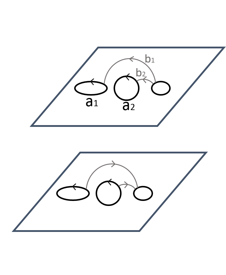
Figure 3: The choice of cycles for a genus $2$ Riemann surface. The $b$ cycles draw a path, one part of which is on the front side and the other on the back side. The $a$ cycles are drawn exactly on the contours connecting the front and back sides.

Let us make note of the non-trivial cycles on the different models of Riemann surfaces we have defined. If the the interface has more than one connected component, the topology of the Riemann surface becomes non-trivial, in that there are cycles which cannot smoothly be contracted to a point. Two cycles are inequivalent if they cannot be deformed one onto the other smoothly. If the interface has $g+1$ connected components, then we may define $g$ such non-trivial inequivalent cycles as $g$ of the $g+1$ connected components. The last connected component is actually equivalent to the union of the first $g$, and thus may not be considered independent. These $g$ cycles are denoted by $a_{j}$, with $j=1,\dots,g$. In addition, $g$ independent cycles, $b_{j}$, may be defined, which intersect the cycles $a_{j}$, respectively, with intersection number $1$. This fact is written formally as:

$$a_{i}\cdot b_{j}=\delta_{i,j}.$$ (3.8)

On the Schottky double, the path of the cycle $b_{j}$ may be considered to start on the front side on the $g+1$ connected component of the interface, then continues to the back side intersecting cycle $a_{j}$ finally connecting to the starting point through the back side. The situation is shown in Fig. 3.

Finally let use describe how the Hamiltonians, $H_{k}$, $\bar{H}_{k}$, are determined by the Riemann surface $\mathcal{D}$ (or equivalently $\mathcal{A}$). The Hamiltonians, $H_{k},$ are multi-valued functions on the Riemann surface. Their derivatives with respect to $z,$ are single-valued, due to Eqs. (2.41), (2.29) and the single-valuedness of the Schwarz function. Let us define

$$H^{(R)}_{k}=\frac{H_{k}+\bar{H}_{k}}{2},\quad H^{(I)}_{k}=\frac{H_{k}-\bar{H}_{k}}{2\imath},$$ (3.9)

which are the Hamiltonians conjugate to the real and imaginary parts of $t_{k}$, respectively. Denote the real and imaginary parts of $t_{k}$ by $t_{k}^{(R)}$ and $t_{k}^{(I)},$ respectively. We shall use the convention that $H_{0}=H/2$, where by $H_{0}^{(R)}=0,$ $H_{0}^{(I)}=H/2.$

The following are well-defined (single-valued) meromorphic differentials on the Riemann surface:

$$dH_{k}^{(R/I)}=\frac{\partial H_{k}^{(R/I)}}{\partial z}dz=\frac{\partial S}{\partial t_{k}^{(R/I)}}dz.$$ (3.10)

Due to (2.44) and (2.41), the differnetial $dH^{(R/I)}_{k}$ has a pole of order $k+1$ at infinity. Indeed:

$$dH_{k}^{(R)}=-\frac{(k-1)}{2}\frac{ds}{s^{k+1}}+O(1/s^{2}ds),\quad dH_{k}^{(I)}=\mp\frac{(k-1)}{2\imath}\frac{ds}{s^{k+1}}+O(1/s^{2}ds)$$ (3.11)

where $s=z^{-1}$ is the local parameter around infinity and the $\pm$ sign in the expansion of $dH^{(I)}_{k}$ is to be taken respectively with whether the expansion is around $\infty_{\uparrow}$ or $\infty_{\downarrow}$. The differential of the Hamiltonians have no further singularities. This last fact can be surmised from (3.10) and (2.19).

A meromorphic differential with specified singularities, such as prescribed by Eq. (3.11), is unique up to an addition of a holomorphic differential, of which there are $g$ on a genus $g$ Riemann surface. Since we can add to $dH_{k}^{(R/I)}$ any linear combination of them with complex coefficients, the space of differentials obeying (3.11) is $2g$ dimensional over $\mathds{R}$. To fix $dH_{k}^{(R/I)}$ completely, one may explore the integral over any cycle of such a differential. We first note that Eq. (2.31) implies that $\oint S(z)dz$ over any cycle is purely imaginary (set $a=b$ in that equation). This fact, when combined with (3.10) gives:

$${\rm Re}\oint_{a_{j}}dH^{(R/I)}_{k}={\rm Re}\oint_{b_{j}}dH^{(R/I)}_{k}=0.$$ (3.12)

This constitutes $2g$ real constraints on $dH^{(R/I)}_{k},$ which completely fix the ambiguity in determining them for any $k$. This means that $dH_{k}$ can also be fixed uniquely given $\mathcal{D}$ or equivalently, $\mathcal{A}$. As a consequence we shall write in the following $H_{k}(\mathcal{A})$ in occasions where we shall want to stress that the Hamiltonians are determined from the Riemann surface.

4 Dispersive Quantization and the two dimensional Toda lattice

We shall now want to proceed and quantize the Laplacian growth dynamics, eventually obtaining quantum field theory, with the aim of using methods of integrable and conformal field theory to gain better understanding of the fractal patterns in Laplacian growth. The program of quantization requires in this case two steps. The first step is removing the dispersionless limit from the two dimensional reduced dispersionless Today hierarchy that was presented above as the hierarchy determining Laplacian growth. This gives a classical nonlinear integrable system, the (dispersionful) two dimensional Toda lattice. Formally, the procedure is very similar to quantization, thus it is dubbed here as ‘dispersive quantization’, although it connects to classical problems. It is only then that we can apply the second step, that of physical quantization, to obtain a quantum field theory.

4.1 The two dimesional Toda Hierarchy

The two dimensional Toda hierarchy [18], is an integrable system of nonlinear equations generalizing the more familiar Toda lattice. The latter being a one dimensional system of springs, having exponential force law $F=F_{0}\cdot(e^{-\Delta x/x_{0}}-1)$, where $F$ is the force that the string exerts when it is extended a distance $\Delta x.$ The nonlinear equation is the Newton equation for the springs:

$$m\frac{d^{2}x_{n}}{dt^{2}}=F_{0}\cdot\left(e^{\frac{x_{n-1}-x_{n}}{x_{0}}}-e^{\frac{x_{n}-x_{n+1}}{x_{0}}}\right).$$ (4.1)

The two dimensional Toda lattice, despite the name, does not generalize the problem of exponential springs to two dimensions, but is rather a formal generalization, in which time itself is treated as a complex variable:

$$\frac{\partial x_{n}}{\partial t_{1}\partial\bar{t}_{1}}=e^{{x_{n-1}-x_{n}}}-e^{{x_{n}-x_{n+1}}}.$$ (4.2)

Here we have set $m$, $F_{0}$ and $x_{0}$ to unity, as the physical interpretation in terms of springs was already lost when we complexified time, and so there is no real use of keeping track of physical units.

The equation of motion for Laplacian growth, when treated as equations determining the evolution of a algebraic Riemann surface, are identical to the equations that are obtained by considering the slow time modulation of the two dimensional Toda lattice hierarchy. Here one assumes that a solution to the two dimensional Toda lattice has the property that it is rapidly oscillating in time (which itself a complex parameter, denoted here by $t_{1}$), in such a way that the envelope of the oscillations varies on a much larger scale than the period of oscillations. If one parametrizes the envelope of oscillations using the correct variables, the equations for these parameters acquire an elegant form, which resemble a semiclassical limit of the full hierarchy. In the present case these semiclassical equations are Eqs. (2.54), defining the Laplacian growth evolution, while the equations for the two dimensional Toda hierarchy are obtained by replacing the Hamiltonians $H_{k}$ by differential operators and the Poisson brackets by commutators. This section, together with appendices A,B, C, is devoted to showing how this connection, described above in heuristic terms, may be derived rigorously.

We must first define the whole two dimensional Toda lattice hierarchy, with its infinite number of complex times, and the respective Hamiltonians. The hierarchy may be defined[18] making use of a Lax operator matrix, $L.$ For the two dimensional Toda lattice, $L$ is an infinite matrix depending on the times, having the property:

$$L_{nm}=0\quad{\rm for}\quad m>n+1.$$ (4.3)

Each time $t_{l}$ has associated with it a Hamiltonian $L^{(l)}$ with matrix elements:

$$L^{(l)}_{mn}=\left\{\begin{array}[]{lr}(L^{l})_{mn}&m>n\\ \frac{1}{2}(L^{l})_{mn}&m=n\\ 0&m<n\end{array}\right.,$$ (4.7)

here, e.g., $(L^{l})_{mn}$ is the $mn$ element of the matrix $L$ raised to the power $l$. The time $\bar{t}_{l}$, has the $-L^{(l)\dagger}$ as the associated Hamiltonian. Note the similarity of (4.7) with (2.34), (2.36).

The nonlinear equations of the hierarchy may be obtained by demanding:

$$\frac{\partial L}{\partial t_{k}}=\left[L,L^{(k)}\right],\quad\frac{\partial L}{\partial\bar{t}_{k}}=-\left[L,L^{(k)\dagger}\right].$$ (4.8)

As a consequence[19] of (4.8) and the definition of $L^{(l)}$, the zero-curvature conditions hold:

$$\frac{\partial L^{(l)}}{\partial t_{k}}-\frac{\partial L^{(k)}}{\partial t_{l}}-[L^{(l)},L^{(k)}] =0$$ (4.9)

$$\frac{\partial L^{(l)\dagger}}{\partial t_{k}}+\frac{\partial L^{(k)}}{\partial\bar{t}_{l}}-[L^{(l)\dagger},L^{(k)}] =0.$$ (4.10)

We shall be interested in a special reduction of the two dimensional Toda hierarchy. Namely, we shall assume the the Lax operator obeys the following condition:

$$[L,L^{\dagger}]=1.$$ (4.11)

In the dispersionless limit this equation becomes (2.21).

To demonstrate how (4.9), (4.10), give rise to a whole hierarchy of nonlinear integrable partial differential equations, let us derive the first member of the hierarchy, Eq. (4.2), from them. First note that any matrix satisfying (4.3) may be written as:

$$L=\sum_{m=-\infty}^{1}a^{(1)}_{m}(\hat{t})e^{m\hat{p}},$$ (4.12)

where $\hat{t}$ acting on a vector $\vec{\psi}$, whose elements are $\psi_{n}$ gives a vector whose elements are $n\psi_{n}$, while the operator $e^{m\hat{p}}$ when acting on the same vector gives a vector whose elements are $\psi_{n+m}$:

$$(\vec{\psi})_{n}=\psi_{n},\quad(\hat{t}\vec{\psi})_{n}=n\psi_{n},\quad(e^{m\hat{p}}\vec{\psi})_{n}=\psi_{m+n}.$$ (4.13)

Note the similarity between Eq. (4.12) with (2.12). In fact the latter equation is the semiclassical limit of the former if we assume that in the limit $\hat{p}\to\imath\varphi$. The similarity between the dispersionless limit (the limit in which one describes the modulations of fast oscillating solutions) and a semiclassical limit, will present itself repeatedly below. The rigorous basis for the similarity will be treated in the next subsections, supplemented by the appendices.

From Eqs. (4.12), (4.7) one may obtain $L^{(1)}$, as follows:

$$L^{(1)}=a^{(1)}_{1}(\hat{t})e^{\hat{p}}+\frac{a^{(1)}_{0}(\hat{t})}{2}.$$ (4.14)

Setting $k=l=1$ in (4.10) one obtains the equation:

$$\frac{1}{2}\left(\frac{\partial a^{(1)}_{0}(\hat{t})}{\partial\bar{t}_{1}}+\frac{\partial\bar{a}^{(1)}_{0}(\hat{t})}{\partial t_{1}}\right)+e^{-\hat{p}}\frac{\partial\bar{a}^{(1)}_{1}(\hat{t})}{\partial t_{1}}+\frac{\partial a^{(1)}_{1}(\hat{t})}{\partial\bar{t}_{1}}e^{\hat{p}}+=\left|a^{(1)}_{1}(\hat{t}-1)\right|^{2}-\left|a^{(1)}_{1}(\hat{t})\right|^{2}+$$ (4.15)

$$+e^{-\hat{p}}\frac{\bar{a}^{(1)}_{1}(\hat{t})a^{(1)}_{0}(\hat{t})-\bar{a}^{(1)}_{1}(\hat{t})a^{(1)}_{0}(\hat{t}+1)}{2}+\frac{a^{(1)}_{1}(\hat{t})\bar{a}^{(1)}_{0}(\hat{t})-a^{(1)}_{1}(\hat{t})\bar{a}^{(1)}_{0}(\hat{t}+1)}{2}e^{\hat{p}}.$$

For the operator on the left hand side to be equal to the operator on the right hand side, the free terms (the terms in the brackets on the left hand side and the first two terms on the right hand side) on the right and left hand sides must be equal, as well as the coefficient of $e^{\hat{p}}$ and $e^{-\hat{p}}$, on both sides of the equation, respectively.

To obtain (4.2), one writes:

$$a^{(1)}_{1}(n)=e^{\imath\theta_{n}}e^{\frac{x_{n}-x_{n+1}}{2}}.$$ (4.16)

The the equation relating the coefficient of $e^{\hat{p}}$ and $e^{-\hat{p}}$ on both sides of (4.15) lead to the same equation:

$$-\imath 2\frac{\partial\theta}{\partial t_{1}}+\frac{\partial}{\partial t_{1}}(x_{n}-x_{n+1}) =a^{(1)}_{0}(n)-a^{(1)}_{0}(n+1)$$ (4.17)

$$\frac{\partial a^{(1)}_{0}(n)}{\partial\bar{t}_{1}}+\frac{\partial\bar{a}^{(1)}_{0}(n)}{\partial t_{1}} =e^{x_{n-1}-x_{n}}-e^{x_{n}-x_{n+1}}$$ (4.18)

Adding the $\bar{t}_{1}$ derivative of (4.17) to its complex conjugate, one obtains:

$$\frac{\partial^{2}}{\partial t_{1}\partial\bar{t}_{1}}(x_{n}-x_{n+1})=e^{x_{n-1}-x_{n}}+e^{x_{n+1}-x_{n+2}}-2e^{x_{n}-x_{n+1}},$$ (4.19)

which is just what is obtained by subtracting Eq. (4.2) from the same equation when $n$ is shifted up by $1$, (that is $n\to n+1$). Namely, if we assume that $x_{n}\to 0$ fast enough as $n\to\pm\infty$, then Eq. (4.19) is equivalent to (4.2), since in that case we can use, e.g., $x_{n}=\sum_{m=n}^{\infty}x_{m}-x_{m+1}.$

4.2 Multi-Periodic Solutions

As mentioned above, the reduced dispersionless two dimensional Toda lattice hierarchy, which determines the evolution Laplacian growth can be obtained by taking the dispersionful reduced two dimensional Toda lattice hierarchy and considering slowly modulated waves. In order to be able to discuss these modulated waves, we must introduce the unmodulated periodic solutions. In particular we must discuss how these are constructed. To do this it is useful to make use of the Baker Akhiezer function[20].

The Baker Akhiezer function, is an eigenfunction of the Lax operator, with complex eigenvalue $z$:

$$L\psi=z\psi.$$ (4.20)

The time dependence of $\psi$ is defined naturally using the Hamiltonians:

$$\frac{\partial\psi}{\partial t_{k}}=L^{(l)}\psi,\quad\frac{\partial\psi}{\partial\bar{t}_{k}}=-L^{(l)\dagger}\psi.$$ (4.21)

For each $z$ there may be several eigenfunctions of $L$. Suppose that, generically, there are $m$ of these eigenfunctions for each $z$. We may take $m$ copies of the complex plane $\mathds{C}$ and assign to each copy one of the eigenfunctions. It turns out that there is a large class of $L$’s such that by drawing branch cuts on the different sheets and gluing the sheets together along the branch cuts, the function $\psi$ becomes a smooth function of $z$, except at infinity, and at a set of discrete poles. In fact, Krichever [21] has shown that an effective way to construct multi-periodic solutions is to start with an algebraic Riemann surface, and define the Baker-Akhiezer function according to some analytic conditions (see also Ref. [22] for an overview of this subject). The Lax matrix $L$, can then be constructed from the knowledge of the Baker-Akhiezer function. Since the elements of the matrix $L$ are the nonlinear fields of of the two dimensional Toda hierarchy, the lax matrix also encodes solutions to the nonlinear integrable equation.

If the algebraic Riemann surface in section admits an anti-holomorphic, $\tau$, then the Riemann surface can be given the structure of a Schottky double. Anticipating the connection to the Riemann surfaces we encountered in Laplacian growth, we assume the existence of such a anti-holomorphic involution and the problem of constructing multi-periodic solutions thus becomes the problem of constructing Baker-Akhiezer functions on a  given Schottky double.

The details of how to define a Baker-Akhiezer function from a set of analytic properties is given in appendix A. The fact that such a function then solves (4.21) is then shown in appendix B. The information pertinent to the sequel is that for each Schottky double a procedure yields a multi-periodic solution of the form:

$$u_{m}(t_{0})=f_{m}\left(\sum_{k=0}^{\infty}t_{k}\vec{\omega}_{k}+\bar{t}_{k}\vec{\bar{\omega}}_{k}\right),$$ (4.22)

where $\vec{\omega}_{k}$ are $g$ dimensional complex vectors and $f_{m}$ are functions from $\mathds{C}^{g}$ to $\mathds{C}$, which are periodic with periods $\hat{e}_{i}$ and $\bm{B}\hat{e}_{i}$:

$$f_{m}(\vec{v}+\hat{e}_{i})=f_{m}(\vec{v}),\quad f_{m}(\vec{v}+\bm{B}\hat{e}_{i})=f_{m}(\vec{v}).$$ (4.23)

Here $\hat{e}_{i}$ is the unit vector in the $i$-th direction, $(\hat{e}_{i})_{j}=\delta_{ij}$, and $\bm{B}$ is a $g$ by $g$ matrix. Many more details are given in appendices A and B. However, the main message of Eq.(4.22) is that a complicated multi-periodic solution of this form may be obtained from a given Schottky double. In fact, $f_{m}$ is given as a combination of Riemann theta functions associated with the Riemann surface.

4.3 Modulations Equations

Given a multi-periodic solution, corresponding to some Schottky double, or equivalently, to a algebraic Riemann surface, one may consider the effect of applying any perturbation to the nonlinear equations. The effect of such a perturbation would be to slowly change the nature of the multi-periodic solution. Namely, the amplitude, phase, average value and frequency would change. After a while, the solution would be described by a different Schottky double, than the one describing the solution at initial times. We may describe the modulation of the multi-periodic wave as dynamics of the Schottky double or the algebraic curve.

The form of the dynamics of the Schottky double naturally depends on perturbation applies. It turns out, however, that if the strength of the perturbation is sent to zero, the original, unperturbed, solution is not recovered. In other words, the limit of vanishing perturbation is singular. Nevertheless, the limit of zero perturbation is universal, in that for sufficiently well behaved perturbations, taking the amplitude of the perturbation to zero yields the same universal Whitham dynamics on Schottky doubles. This leads to the interesting situation in which there is a natural dynamics defined on Schottky doubles or, equivalently, algebraic curves. For the case of the reduced two dimensional Toda lattice, the universal dynamics obtained is that of Laplacian growth, which was already described as the dynamics of the algebraic Riemann surface $\mathcal{A}$.

Whitham [23, 24, 25, 26, 27] developed some of the first tools to describe such universal modulated dynamics for nonlinear wave. Flaschka, Forest and McLaughlin connected this evolution to concepts in algebraic geometry, while Krichever [28] was able to derive the dynamics rigorously making use of an averaging method that he had devised. The resulting dynamics has an integrable structure (as we have seen in Laplacian growth above). Such dynamics are sometimes called dispersionless hierarchies or Whitham hierarchies. Appendix C is devoted to a review of Krichever’s work[28], following the more accessible presentation of Ref. [27, 23].

The modulation equations obtained by this procedure are Eqs. (2.51). They are obtained by essentially averaging the zero curvature conditions, Eqs. (4.9), (4.10), with the Baker-Akhiezer function, and its adjoint over many periods of the multi-periodic solution, but on a scale much smaller than the typical scale of modulation. The details are given in appendix C.

Let us note that Eqs. (2.51) can be solved by taking a Riemann surface which is times independent. Indeed, as was describe in section 3, the Hamiltonians $H_{k}$ can be found by considering that $dH_{k}$ is a unique differential on the Riemann surface, such that if the Riemann surface does not change then both left and right hand side of (2.51) are zero. Nevertheless, such a solution is obviously not a solution of the Laplacian growth problem. Mathematically, we see this by noting that we are seeking solutions in which there is a Schwarz function that generates this Hamiltonian (Eq. (2.41)) and obeys the unitarity condition (Eq. (2.14)). The fact that given initial conditions two solutions exist, is related to the fact that the Whitham equations are a singular limit obtained by adding a perturbation to the equations and sending this perturbation to zero. The solution which corresponds to Laplacian growth is the non-trivial solution in which the Riemann surface is time dependent and in which the unitarity condition is preserved by the evolution.

5 The Classical Korteweg-de Vries Limit

After discussing how to remove the dispersionless limit from the integrable structure of Laplacian growth to obtain the (dispersionful) reduced two dimensional Toda lattice hierarchy, we would like to quantize the latter. A lot more is known, though, on the quantization of Korteweg-de Vries equation than the quantization of the two dimensional Toda lattice. In fact, quantum Korteweg-de Vries is the integrable structure underlying conformal field theory, which makes this quantum integrable system very appealing, due to the rich structure and the applicability of results of the representation theory of the Virasoro algebra.

Due to these consideration, we opt to first treat a limit of Laplacian growth, which has the integrable structure of Korteweg-de Vries associated with it [10]. Only then will we consider quantization. The advantage of this approach is that we will be able to use results from conformal field theory after quantization, the drawback is that it is not clear to what extent the fractal nature of the growth extends to the Korteweg-de Vries limit.

5.1 Narrow Finger Limit of Hele-Shaw Flows

If one focuses on a region around a Hele-Shaw finger, the integrable structure of the two dimensional Toda lattice simplifies in the limit of a very thin and long finger. Let us orient the $x$ axis to point in the long direction of the finger (see Fig. 4). The Korteweg-de Vries limit occurs when the finger is symmetric to reflection across the $x$-axis and when the curve is described at intermediately large and negative $x$ as

$$y=y_{0}\left(\frac{x}{x_{0}}\right)^{J-3/2}+\dots,$$ (5.1)

where $x_{0}\gg y_{0}$, so that the finger is long and narrow. Eq. (5.1) describes the shape of the finger at $x\sim x_{0}$, and may have more complicated features at $x\ll x_{0}$. Nevertheless, it is assumed that throughout the region, for all points on the interface, $y\ll x$. Due to this $f_{t}(\imath\varphi)$ is approximately real in the entire region.

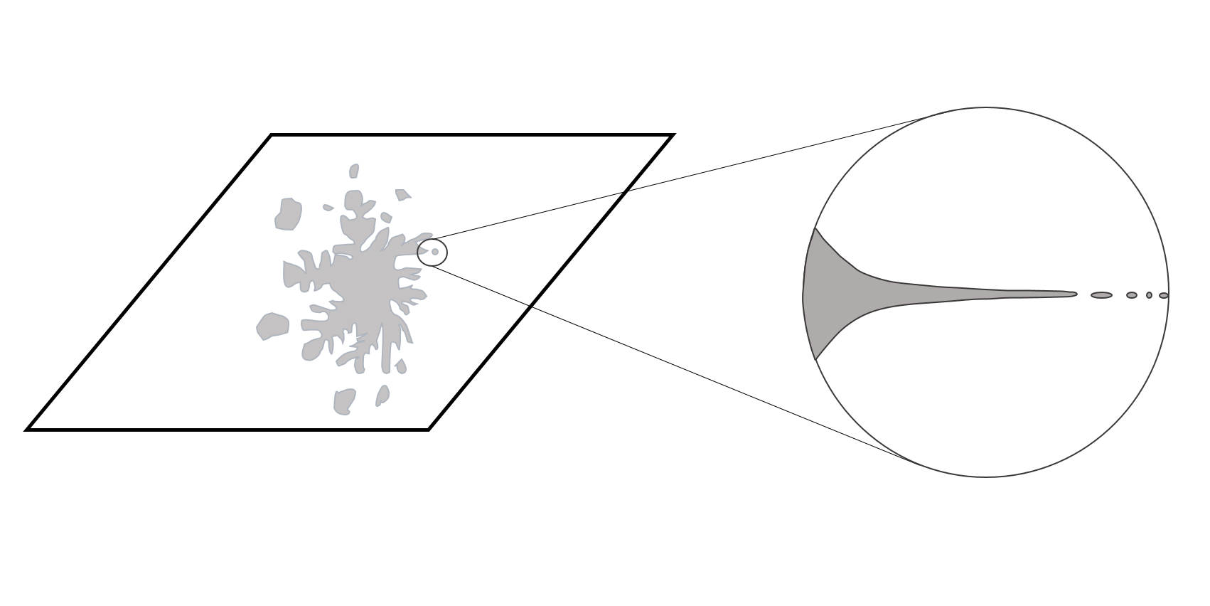
Figure 4: A small part of the droplet is magnified, to reveal a long and narrow, possibly multi-connected, finger, symmetric with respect to reflections about the real axis.

The Korteweg-de Vries description of the finger holds for any rapid evolution of the interface at $|x|\ll x_{0}$, while the asymptotic behavior at $x\sim x_{0}$, Eq. (5.1), does not change. Namely, in Eq. (5.1), we may assume that $x_{0}$ and $y_{0}$ are time independent. Furthermore, since the Korteweg-de Vries description only holds for the confined region $x\ll x_{0},$ we may assume that Eq. (5.1) describes the asymptotic behavior of the not only at $x\sim x_{0}$ but all the way to $x\to-\infty.$

To describe such a finger, we first define a re-scaled and shifted $\varphi$ and $t$ given by $\tilde{\varphi}$ and $\tilde{t}$, respectively. Namely, we define $\tilde{\varphi}(\varphi)=a\varphi+b$, $\tilde{t}=\alpha t+\beta$, where the way $a,b,\alpha,\beta$ are chosen will be described below. Let:

$$l_{\tilde{t}}(\tilde{\varphi})=\frac{f_{t(\tilde{t})}(\imath\varphi(\tilde{\varphi}))+\bar{f}_{t(\tilde{t})}(-\imath\varphi(\tilde{\varphi}))}{2},\quad h_{\tilde{t}}(\tilde{\varphi})=\frac{f_{t(\tilde{t})}(\imath\varphi(\tilde{\varphi}))-\bar{f}_{t(\tilde{t})}(-\imath\varphi(\tilde{\varphi}))}{2\imath}.$$ (5.2)

We may now expand $l_{\tilde{t}}$, $h_{\tilde{t}}$ as a Laurent series in $\tilde{\varphi}$ around infinity, such that the asymptotics described in Eq. (5.1) is recovered.The simplest choice is to take:

$$l_{\tilde{t}}=\tilde{\varphi}^{2}+\sum_{j=-\infty}^{0}\tilde{a}^{(1)}_{j}\tilde{\varphi}^{2j},$$ (5.3)

and

$$h_{\tilde{t}}=\frac{y_{0}}{x_{0}^{J-3/2}}\tilde{\varphi}^{2J-3}+O\left(\tilde{\varphi}^{2J-1}\right).$$ (5.4)

The choice of $a$ and $b$ in $\tilde{\varphi}(\varphi)=a\varphi+b$, is made such that the free term in (5.3)  is missing and the highest order term has unit pre-factor. The fact that $l_{\tilde{t}}$ has only even powers in an expansion in $\tilde{\varphi}$ and $h_{\tilde{t}}$ only odd powers, corresponds to the symmetry of the finger with respect to reflections across the real axis. Indeed, together with (5.4), the reflection symmetry is effected by $\tilde{\varphi}\to-\tilde{\varphi}$, whereby $l_{\tilde{t}}\to l_{\tilde{t}}$, while $h_{\tilde{t}}\to-h_{\tilde{t}}$. The fact that this way to respect the reflection symmetry is actually implemented by the conformal map $f_{t}$ in the asymptotic region, is not guaranteed. Nevertheless, it may be expected to hold fairly generally, when the shape of the interface away from the finger does not induce a strongly asymmetric pressure field on the finger. We shall not dwell on this point, as we are mainly interested in the existence of the Korteweg-de Vries limit under some conditions, rather than demanding that it hold under generic conditions.

Instead of the Schwarz function it is more appropriate to define the following combination:

$$\quad y(x)=h_{\tilde{t}}(\tilde{\varphi}_{\tilde{t}}(x)),\quad$$ (5.5)

where $\tilde{\varphi}_{\tilde{t}}(x)$ is the inverse function of $l_{\tilde{t}}$:

$$l_{\tilde{t}}(\tilde{\varphi}_{\tilde{t}}(x))=x.$$ (5.6)

The function $y(x)$ is the analytic continuation in $x-$plane of a function which gives the $y$ coordinate of the finger as a function of the $x$ coordinate, for $x$ that belongs to the droplet. Such $x$’s that below to the finger form segments on the real axis. These segments are branch cuts for the function $y(x)$. If one approaches the branch cut from above or below one obtains the $\pm y(x)$, respectively. Namely as $x$ approaches the real axis we have $y(\bar{x})=-y(x)$. Since $y$ is real we can take the complex conjugate of the left hand side of this equation and obtain:

$$\bar{y}(x)=-y(x).$$ (5.7)

This equation holding for $x$ approaching the real axis.

Around the contour we have ostensibly $y(x)=\sum_{n}a_{n}(\sqrt{x-\lambda_{i}})^{n}$. To obey (5.7), $a_{2n}$ have to be purely imaginary, but $y$ is real on the real axis and so $a_{2n}=0$. Thus, $y(x)$ has only odd powers of $\sqrt{x-\lambda_{i}}$ which implies that $y^{2}(x)$ is regular, as a function of $x$, everywhere in the complex plane. Namely, it is an entire function. In addition, $y^{2}(x)\sim x^{2J-3}$ as $x\to\infty,$ which, together with the fact that it is entire, suggests that it is a polynomial. Considering that the zeros of this polynomial are the branch points, one obtains:

$$y^{2}(x)=\prod_{i=1}^{2g+1}(x-\lambda_{i}).$$ (5.8)

This equation describes a Riemann surface, through a complex curve. Curves which are defined through $y^{2}=P_{n}(x)$, where $P_{n}$ is a polynomial, are called hyper-elliptic. Thus, in the Korteweg-de Vries limit, the Riemann surface is a hyper-elliptic curve.

Given the definition, Eq. (5.2), of $l_{\tilde{t}}$ and $h_{\tilde{t}}$, Eq. (2.21) implies the following Poisson bracket for these objects:

$$\{l_{\tilde{t}},h_{\tilde{t}}\}=1,$$ (5.9)

where here the choice of $\alpha$ in $\tilde{t}=\alpha t+\beta$ is made as to have $1$ on the right hand side. The choice of $\beta$ remains arbitrary. Eqs. (5.3), (5.4) leads to the following expansion for $y$:

$$y(x)=\sum_{k=1}^{J}\tilde{t}_{2k+1}x^{k-1/2}+O(z^{-3/2}).$$ (5.10)

with $\tilde{t}_{1}=\tilde{t}$. All the $\tilde{t}_{2k+1}$ are real parameters, as the symmetry of the finger dictates.

In a manner following closely to the way in which Eq. (2.29) was derived from (2.21), one may derive from (5.9) the following equation:

$$\frac{\partial y(x)}{\partial\tilde{t}}=\frac{\partial\tilde{\varphi}_{\tilde{t}}(x)}{\partial x}.$$ (5.11)

Define now the Hamiltonians

$$\tilde{H}_{2k+1}=\left(x_{\tilde{t}}^{k+1/2}\right)_{\tilde{+}},$$ (5.12)

where the definition of $g(\tilde{\varphi})_{\tilde{+}}$ , for any function $g(\tilde{\varphi})=\sum_{k=-\infty}^{\infty}\alpha_{k}\tilde{\varphi}^{k}$ is as follows:

$$g_{\tilde{+}}=\frac{\alpha_{0}}{2}+\sum_{k=1}^{\infty}\alpha_{k}\tilde{\varphi}^{k}.$$ (5.13)

Assume

$$\frac{\partial l_{\tilde{t}}}{\partial\tilde{t}_{k}}=\{x_{\tilde{t}},\tilde{H}_{k}\},\quad\frac{\partial h_{\tilde{t}}}{\partial\tilde{t}_{k}}=\{h_{\tilde{t}},\tilde{H}_{k}\},$$ (5.15)

for $k$ odd. Then,

$$\frac{\partial y(x)}{\partial\tilde{t}_{k}}=\left.\frac{\partial l_{\tilde{t}}(\tilde{\varphi})}{\partial\tilde{t}_{k}}+\frac{\partial l_{\tilde{t}}(\tilde{\varphi})}{\partial\tilde{\varphi}}\frac{\partial\tilde{\varphi}_{t}(x)}{\partial\tilde{t}_{k}}\right|_{\tilde{\varphi}=\tilde{\varphi}_{t}(x)}=$$ (5.16)

$$=\left.\{l_{\tilde{t}},\tilde{H}_{k}\}-\left(\frac{\partial\tilde{l}_{t}(\tilde{\varphi})}{\partial\tilde{\varphi}}\right)^{-1}\frac{\partial l_{\tilde{t}}(\tilde{\varphi})}{\partial\tilde{\varphi}}\frac{\partial\tilde{l}_{t}(\tilde{\varphi})}{\partial\tilde{t}_{k}}\right|_{\tilde{\varphi}=\tilde{\varphi}_{t}(x)}=$$

$$=\left.\frac{\partial\tilde{H}_{k}}{\partial\tilde{\varphi}}/\frac{\partial\tilde{l}_{t}(\tilde{\varphi})}{\partial\tilde{\varphi}}\right|_{\tilde{\varphi}=\tilde{\varphi}_{t}(x)}=\frac{\partial\tilde{H}_{k}}{\partial x}$$ (5.17)

This equation is an evolution equation in time $\tilde{t}_{k}$ for $y$, and has the property that it retains the form (5.10). This shows that the times $\tilde{t}_{k}$ may be viewed as the analogue of the harmonic moments in the narrow finger limit. First, each $\tilde{t}_{k}$ is conserved when any on of the other times is changed and secondly, the $\tilde{t}_{k}$ are quantities characterizing the shape of the interface. Indeed, the function $y(x)$, for which the $\tilde{t}_{k}$ are Laurent coefficients, can be found by directly from the shape of the interface, as it is the analytic continuation in the complex $x-$plane of the function which gives the $y$ coordinate of the interface given the $x$ coordinate.

5.2 Dispersive Quantization of Korteweg-de Vries

Just as we have applied ‘dispersive quantization’ the the dispersionless limit of the two dimensional Toda lattice equations, we shall now be interested in applying the same procedure the the dispersionless Korteweg-de Vries equations (5.15). We shall at this point do away with the tildes over the time, over the $\varphi$ variable, and the Hamiltonians, since we shall not treat the two dimensionless Toda anymore, and as such there should be no confusion about whether the objects discussed belong to the Korteweg-de Vries or the two dimensional Toda hierarchies.

The Korteweg-de Vries hierarchy may be defined (See Ref. [29] and references therein) by considering the Lax operator, $L$, a differential operator in $t_{1}$, given by:

$$\hat{L}=\partial_{t_{1}}^{2}+\frac{u(t_{1})}{6}.$$ (5.18)

One may write the square root of $\hat{L}$ as a formal power series in $\partial_{t_{1}}$:

$$\hat{L}^{1/2}=\partial_{t_{1}}+\sum_{m=0}^{\infty}b_{m}(t_{1})\partial_{t_{1}}^{-m},$$ (5.19)

where $\partial_{t_{1}}^{-m}$ is the formal inverse of $\partial_{t_{1}}$ raised to the power $m$. The function $b_{m}(t_{1})$ can be found, order by order, by demanding $\hat{L}^{1/2}\hat{L}^{1/2}=\hat{L}$.

A set of Hamiltonians are then given by

$$\hat{H}_{2k+1}=\left(\hat{L}^{1/2}\hat{L}^{k}\right)_{+},$$ (5.20)

where the $(\hat{L}^{k+1/2})_{+}$ denotes only positive powers of $\partial_{t_{1}}$ in the expansion of $L^{1/2}\hat{L}$, which itself contains both positive and negative powers. The equations for the hierarchy follow from the Lax equations:

$$\partial_{t_{k}}\hat{L}=[\hat{L},\hat{H}_{k}]1$$ (5.21)

The dispersionless limit of this problem becomes the problem that has been discussed in the previous subsection. To show this one may follow much the same as described in for the two dimensional Toda lattice. In fact the result may be obtained by taking an appropriate limit of that procedure. Namely, the long and narrow finger limit, in which the Riemann surface becomes hyperelliptic, and only real odd times describe the evolution. As such, we shall not repeat those steps. We note, that the original literature cited here on the matter [28, 30, 31] either deals directly with the Korteweg-de Vries problem, or with close relatives, which are easily reduced to the Korteweg-de Vries problem – mainly the Kadomtsev-Petviashvili hierarchy.

The first member of the hierarchy gives the tautology $\partial_{t_{1}}u=\partial_{t_{1}}u.$The first non-trivial member of the hierarchy is given by:

$$4\partial_{t_{3}}u=\partial_{t_{1}}^{3}u+u\partial_{t_{1}}u.$$ (5.22)

Alternative to the Lax construction, this equation may be obtained by defining the following Poisson brackets:

$$\{u(x),u(y)\}=2(u(x)+u(y))\delta^{\prime}(x-y)+\delta^{\prime\prime\prime}(x-y),$$ (5.23)

and allowing for evolution with the Hamiltonian:

$$H_{3}=\frac{1}{8}\oint u^{2}(t_{1})dt_{1},$$ (5.24)

upon which, Eq. (5.22) becomes equivalent to:

$$\partial_{t_{3}}u=\{u,H_{3}\}.$$ (5.25)

The tautological equation $\partial_{t_{1}}u=\partial_{t_{1}}u$ is generated by $H_{1}$ given by

$$H_{1}=\int u(t_{1})dt_{1}.$$ (5.26)

All higher order flows defined by (5.21) may be obtained using the Poisson bracket (5.23) by defining appropriate Hamiltonians (See Ref. [29] and references therein) .

5.3 Inverse Scattering

The method of inverse scattering was first invented for the Korteweg-de Vries equation[32] and later expanded to become a wide-ranging subject (see, e.g., Ref. [29] and references therein). It is useful to review briefly the inverse scattering method, since it provides a link between the classical multi-periodic solutions to the quantum states one obtains in solving the integrable quantum Korteweg-de Vries equation.

To present the method of inverse scattering, first let us consider the periodic problem. Namely, we consider the problem in which the field $u(t_{1})$ is periodic with period $2\pi$. Next, we consider the Miura transformation:

$$u=-\left(\frac{\partial\phi}{\partial t_{1}}\right)^{2}-\frac{\partial^{2}\phi}{\partial t^{2}_{1}}.$$ (5.27)

The Poisson bracket for the field $\phi$ is then given by:

$$\{\phi(t_{1}),\phi(t_{1}^{\prime})\}=\frac{1}{2}\rm sign(t_{1}-t_{1}^{\prime}),$$ (5.28)

and can be shown to be equivalent to (5.23). Namely, substituting (5.27) into (5.28) one obtains (5.23) up to full derivatives. The latter are determined by requiring that the Poisson bracket of $\phi$ must be obey the Jacobi identity.

The Korteweg-de Vries equation, Eq. (5.22), translates into the following equation for $\phi$:

$$\frac{\partial\phi}{\partial t_{3}}=\frac{\partial^{3}\phi}{\partial t^{3}_{1}}-2\left(\frac{\partial\phi}{\partial t_{1}}\right)^{3},$$ (5.29)

which is a version of the modified Korteweg-de Vries equation (the standard modified Korteweg-de Vries equation is written for the field $v=\phi^{\prime}$).

The equation for $\phi$, Eq. (5.29) can be obtained for a zero curvature condition for a Lax pair. Consider the operators

$$\bm{A}_{\lambda} =\phi^{\prime}\sigma_{z}+\sqrt{\lambda}\sigma_{x},$$ (5.30)

$$\bm{B}_{\lambda} =\sqrt{\lambda}(4\lambda-2\phi^{\prime 2})\sigma_{x}+(\phi^{\prime\prime\prime}+\phi^{\prime}(4\lambda-2\phi^{\prime 2}))\sigma_{z}-2\imath\phi^{\prime\prime}\sqrt{\lambda}\sigma_{y},$$ (5.31)

where the prime denotes derivative with respect to $t_{1}$. Then the equation

$$\left[\frac{\partial}{\partial t_{1}}-\bm{A}_{\lambda},\frac{\partial}{\partial t_{3}}-\bm{B}_{\lambda}\right]=0,$$ (5.32)

becomes equivalent to (5.29) as can be ascertained by computing the commutator explicitly.

Eq. (5.32), which is equivalent to the dynamic equation of $\phi$, Eq. (5.29), has exactly the required form to serve as the consistency condition required for there to be a solution, $\vec{\psi}$, to the equations:

$$\left(\frac{\partial}{\partial t_{1}}-\bm{A}_{\lambda}\right)\vec{\psi}=0$$ (5.33)

$$\left(\frac{\partial}{\partial t_{3}}-\bm{B}_{\lambda}\right)\vec{\psi}=0$$ (5.34)

where $\vec{\psi}$ is a two dimensional vector. The significance of this fact is that one may approach the problem of finding solutions of the modified Korteweg-de Vries equation, Eq. (5.29), or equivalently the Korteweg-de Vries equation, Eq. (5.22), as the problem of constructing solutions to (5.33) and (5.34) as Baker Akhiezer functions as done above. In this section we shall show how the Baker-Akhiezer function is related to the method of separation of variables.

The solution of (5.33) is in fact simple. We may write:

$$\vec{\psi}(t_{1})=\mathscr{P}\left[e^{\int_{0}^{t_{1}}\bm{A}_{\lambda}}\right]\vec{\psi}(0),$$ (5.35)

where $\mathscr{P}$ denotes a path-ordered product. One is lead to define the shift operator:

$$\bm{M}_{\lambda}(t^{\prime}_{1},t_{1})=e^{\int_{t_{1}}^{t_{1}^{\prime}}A_{\lambda}}.$$ (5.36)

The problem of finding Bloch wave-functions $\vec{\psi}(t_{1}+2\pi)=e^{\imath\theta(\lambda)}\vec{\psi}(t_{1}),$ satisfying (5.33) and (5.34) is then the problem of finding eigenvectors of the matrix $\bm{M}_{\lambda}(2\pi,0)$. The object $e^{\imath\theta(\lambda)}$ is called the Bloch multiplier of the Bloch wave-function $\vec{\psi}(t_{1}).$ Note that the first element of $\vec{\psi}$, denoted by $\psi_{1}$, is also Bloch wave-functions for the following equation:

$$(\partial_{t_{1}}^{2}+u(t_{1}))\psi_{1}=\hat{L}\psi_{1}=\lambda\psi_{1},$$ (5.37)

an equation which is easily derived making use of Eqs. (5.33) and (5.27). A Bloch eigenfunction of the Lax operator is the Baker-Akhiezer function. Indeed, the Baker-Akhiezer function is a solution to the spectral problem, where the coefficients appearing in the Lax operator are multi-periodic functions.

A special case in which the eigenvectors of $\bm{M}_{\lambda}(2\pi,0)$ are apparent presents itself for values of $\lambda$ at which $\bm{M}_{\lambda}(2\pi,0)$ happens to be diagonal. The the Bloch wave-functions are given by the standard basis

$$\left(\begin{array}[]{c}1\\ 0\end{array}\right),\left(\begin{array}[]{c}0\\ 1\end{array}\right),$$ (5.42)

up to a times dependent factor. We see that the first element of one of the Bloch function vanishes. Namely the Baker-Akhiezer function vanishes at this $\lambda$ on one of the sheets. The matrix $\bm{M}_{\lambda}$ depends on the times and as such the points $\lambda$ at which this matrix is diagonal also depend on time. Suppose that there are $g$ such points. Indeed, on a Riemann surface of genus $g$ the Baker-Akhiezer function has $g$ zeros (see appendix A). These points form a set of $g$ dynamical variables denoted by $\gamma_{i}$. Another set of dynamical parameter may be taken as the Bloch multiplier associated with the non-vanishing Baker-Akhiezer function at $\gamma_{i}$. Namely we take the upper left element, $\left(\bm{M}_{\gamma_{i}}\right)_{11},$ as a set of $g$ additional dynamical variables. As shown in Ref.[33] and reviewed below, these parameters have a Poisson structure that allows one to treat them as separated variables. We review the computation of these Poisson brackets in the following, by computing the Poisson brackets of the elements of $\bm{M}_{\lambda}(2\pi,0)$ for any $\lambda$ and then specializing to the points where $\bm{M}_{\lambda}(2\pi,0)$ is diagonal.

We wish to find the Poisson brackets of the different elements of $\bm{M}_{\lambda}(2\pi,0).$ Since we are interested in finding the Poisson bracket of any two matrix elements of $\bm{M}_{\lambda}(2\pi,0)$, it is useful to consider the simultaneous operation of taking the tensor product and the Poisson bracket. Namely for any two matrices, $\bm{a}$ and $\bm{b}$, one may consider the object $\{\bm{a}\overset{\otimes}{,}\bm{b}\}$, which is an object which lives in the same space as $\bm{a}\otimes\bm{b}$, and has matrix elements given by:

$$\{\bm{a}\overset{\otimes}{,}\bm{b}\}_{\alpha\beta\gamma\delta}=\{\bm{a}_{\alpha\gamma},\bm{b}_{\beta\delta}\},$$ (5.43)

just as $(\bm{a}\otimes\bm{b})_{\alpha\beta\gamma\delta}=\bm{a}_{\alpha\gamma}\bm{b}_{\beta\delta}$.

From now on we shall denote

$$\bm{M}_{\tau}\equiv\bm{M}_{\tau}(2\pi,0)$$ (5.44)

With this definition we compute:

$$\{\bm{M}_{\lambda}\overset{\otimes}{,}\bm{M}_{\mu}\}=\iint dxdx^{\prime}\bm{M}_{\lambda}(2\pi,x)\otimes\bm{M}_{\mu}(2\pi,x^{\prime})\{\bm{A}_{\lambda}(x)\overset{\otimes}{,}\bm{A}_{\mu}(x^{\prime})\}\bm{M}_{\lambda}(x,0)\otimes\bm{M}_{\mu}(x^{\prime},0)$$ (5.45)

This equation is a consequence of the definition of $\bm{M}$ in terms of $\bm{A}$ (Eq. (5.36)) only, and may be derived by writing $\bm{M}$ in terms of a path ordered product:

$$\bm{M}_{\lambda}=\lim_{N\to\infty}\mathscr{P}\prod_{i}^{N}\left(\mathds{1}+\int_{\frac{2\pi}{N}(i-1)}^{\frac{2\pi}{N}i}\bm{A}_{\lambda}\right),$$ (5.46)

and computing the Poisson brackets that appear in (5.45).

An explicit calculation gives

$$\{\bm{A}_{\lambda}(x)\overset{\otimes}{,}\bm{A}_{\mu}(x^{\prime})\}=\delta^{\prime}(x-x^{\prime})\sigma_{z}\otimes\sigma_{z}$$ (5.47)

Inserting this into (5.45), writing $\delta^{\prime}(x-y)=\frac{\partial_{x}-\partial_{y}}{2}\delta(x-y)$ and integrating by parts, one obtains:

$$\{\bm{M}_{\lambda}\overset{\otimes}{,}\bm{M}_{\mu}\}=$$ (5.48)

$$=\int dx\bm{M}_{\lambda}(2\pi,x)\otimes\bm{M}_{\mu}(2\pi,x)\left[\sigma_{z}\otimes\sigma_{z},\frac{\bm{A}_{\lambda}(x)\otimes\mathds{1}-\mathds{1\otimes}\bm{A}_{\mu}(x)}{2}\right]\bm{M}_{\lambda}(x,0)\otimes\bm{M}_{\mu}(x,0),$$

where here we used the fact that $\bm{M}_{\tau},$ obeys similar equations to those that $\vec{\psi}$ obeys:

$$\partial_{x}\bm{M}_{\tau}(x,x^{\prime})=\bm{A}_{\tau}(x)\bm{M}_{\tau}(x,x^{\prime}),\quad\partial_{x^{\prime}}\bm{M}_{\tau}(x,x^{\prime})=-\bm{M}_{\tau}(x,x^{\prime})\bm{A}_{\tau}(x^{\prime}),$$ (5.49)

whereupon one may substitute $\mu$ or $\lambda$ for $\tau$.

Finally, we need the following identity, which may be obtained by an explicit calculation:

$$\left[\sigma_{z}\otimes\sigma_{z},\bm{A}_{\lambda}(x)\otimes\mathds{1}-\mathds{1\otimes}\bm{A}_{\mu}(x)\right]=\left[\bm{R}_{\sqrt{\lambda/\mu}},\bm{A}_{\lambda}(x)\otimes\mathds{1}+\mathds{1\otimes}\bm{A}_{\mu}(x)\right],$$ (5.50)

where

$$\bm{R}_{\tau}=\frac{\tau+\tau^{-1}}{\tau-\tau^{-1}}\frac{\sigma_{z}\otimes\sigma_{z}}{2}+\frac{2}{\tau-\tau^{-1}}(\sigma_{+}\otimes\sigma_{-}+\sigma_{-}\otimes\sigma_{+}).$$ (5.51)

Substituting (5.50) into (5.48) and making use Eq. (5.49), one may write:

$$\{\bm{M}_{\lambda}\overset{\otimes}{,}\bm{M}_{\mu}\}=$$

$$=\int dx\partial_{x}\left(\bm{M}_{\lambda}(2\pi,x)\otimes\bm{M}_{\mu}(2\pi,x)\bm{R}_{\sqrt{\lambda/\mu}}\bm{M}_{\lambda}(x,0)\otimes\bm{M}_{\mu}(x,0)\right)=$$

$$=\left[\bm{R}_{\sqrt{\lambda/\mu}},\bm{M}_{\lambda}\otimes\bm{M}_{\mu}\right],$$ (5.52)

This is the desired result. In the present, classical, terms, the equation encodes the Poisson brackets between the elements of $\bm{M}$ at different spectral parameters in terms of bilinears of $\bm{M}$ itself. The quantization of these relations will allow to compute the commutations relations for such elements in the same manner.

An almost immediate consequence of (5.52) is that the trace of $\bm{M}_{\lambda}$, denoted as $\bm{T}_{\lambda}$:

$$\bm{T}_{\lambda}={\rm tr}\bm{M}_{\lambda},$$ (5.53)

Poisson commutes

$$\{\bm{T}_{\lambda},\bm{T}_{\mu}\}=0,$$ (5.54)

an equation which is immediately obtained from (5.52) by noting that ${\rm tr}\left[\{\bm{a}\overset{\otimes}{,}\bm{b}\}\right]=\{{\rm tr}[\bm{a}],{\rm tr}[\bm{b}]\}$, just as ${\rm tr}\left[\bm{a}\otimes\bm{b}\right]={\rm tr}[\bm{a}]{\rm tr}[\bm{b}]$.

The relation (5.54) encodes the infinite number of conserved quantities in involution. Indeed, it turns out that the expansion of $\bm{T}_{\lambda}$ around $\lambda\to\infty$, yields the conserved quantities as the coefficients in the Laurent expansion. This proves that they are in involution.

It is customary to define the following matrix elements of the matrix $\bm{M}_{\tau}$:

$$\bm{M}_{\tau}=\left(\begin{array}[]{cc}a_{\tau}&b_{\tau}\\ c_{\tau}&d_{\tau}\end{array}\right).$$ (5.57)

To obtain separated variables one first notes that from (5.52) the following relation may be obtained by taking the appropriate matrix element:

$$\{b_{\lambda},b_{\mu}\}=0.$$ (5.58)

Consider the points at which $\bm{M}_{\tau}$ is diagonal. At these points, denoted by $\gamma_{i}$ we have $b_{\gamma_{i}}=0$. The following is then a consequence of (5.58):

$$\{\gamma_{i},\gamma_{j}\}=0.$$ (5.59)

We have found a set of variables which are in involution. As further dynamical variables one may consider $\Lambda_{i}=a_{\gamma_{i}}$. Referring back to (5.52) and taking the appropriate matrix elements one concludes:

$$\{\Lambda_{i},\Lambda_{j}\}=0,$$ (5.60)

and

$$\{\Lambda_{i},b_{\gamma_{j}}\}=4\delta_{i,j}\Lambda_{i}\gamma_{i}b^{\prime}_{\gamma_{i}},$$ (5.61)

where $b^{\prime}_{\gamma_{i}}=\left.\frac{db_{\tau}}{d\tau}\right|_{\tau=\gamma_{i}}$. Eq. (5.61) may be obtained if we postulate the following Poisson brackets:

$$\{\Lambda_{i},\gamma_{j}\}=4\delta_{i,j}\Lambda_{i}\gamma_{i}.$$ (5.62)

We thus have:

$$\{\Lambda_{i},\Lambda_{j}\}=\{\gamma_{i},\gamma_{j}\}=0,\quad\{\log\Lambda_{i},\log\gamma_{j}\}=\delta_{i,j}.$$ (5.63)

The variables $\log(\gamma_{i})$ and $\log(\Lambda_{i})$ are thus canonical. To show that these are also separated variables, one needs to show that each pair $(\gamma_{i},\Lambda_{i})$ traces out a one dimensional loop, whose shape is independent of all the rest of the canonical variables. Namely, one must show that $\Lambda_{i}$ is a function of $\gamma_{i}$, the function depending only on the conserved quantities. The existence of such a representation is a consequence of the fact that $\Lambda_{i}$ is the Bloch multiplier associated with the Baker-Akhiezer function at $\gamma_{i}$. An explicit expression for the Baker-Akhiezer function is given in appendix A, from which $\Lambda(z)$ may be found. We thus have $\Lambda_{i}=\Lambda(\gamma_{i})$, as required.

6 Quantum Korteweg-de Vries

Having reviewed the classical inverse scattering method, we are able to present the quantum version of which, discovered in Refrs. [11, 12, 13] based on results of Refrs. [14, 15]. More context on the quantum inverse scattering can be found in Ref.  [34] and is also treated briefly in Ref. [29]. We then go on to review the quantization of the Korteweg-de Vries problem based on quantizing the field $u(t_{1})$, which leads to the connection to conformal field theory. An object which bridges the two approaches is given by the form factors, which has a central role in the proposed connection to Laplacian growth.

6.1 Quantum Separation of Variables

The classical separation of variables method for the Korteweg-de Vries problem was achieved by considering the monodromy matrix. Quantum Korteweg-de Vries can be defined by quantizing in the separate variables, in a method suggested by Sklyanin [35]. On defines the quantum analogues of $\gamma_{i}$ and $\Lambda_{j}$ as a set of operator $\hat{\gamma}_{i}$, $\hat{\Lambda}_{i}$, with the following commutation relations:

$$[\hat{\Lambda}_{i},\hat{\Lambda}_{j}]=[\hat{\gamma}_{i},\hat{\gamma}_{j}]=0,\quad\hat{\Lambda}_{i}\hat{\gamma}_{j}=e^{\imath\pi\hbar\delta_{i,j}}\hat{\gamma}_{j}\hat{\Lambda}_{i}.$$ (6.1)

To see that indeed (6.1) is the classical limit of the last equation of (5.63), we write the last equation in (6.1) as:

$$e^{\log(\hat{\Lambda}_{i})+\log(\hat{\gamma}_{k})+\frac{1}{2}[\log(\Lambda_{i}),\log(\hat{\gamma}_{k})]+\dots}=e^{\imath\pi\hbar\delta_{i,j}+\log(\hat{\Lambda}_{i})+\log(\hat{\gamma}_{k})-\frac{1}{2}[\log(\Lambda_{i}),\log(\hat{\gamma}_{k})]+\dots},$$ (6.2)

obtained by using Baker-Campbell-Hausdorff Lemma. Taking the logarithm of both sides, one obtains:

$$[\log\hat{\Lambda}_{i},\log\gamma_{j}]=\delta_{i,j}\imath\pi\hbar+\dots.$$ (6.3)

The semiclassical limit of this equation is indeed (5.63), as desired.

One may find a representation of this algebra by postulating some Hilbert space spanned by the joint eigenvectors of all the $\hat{\gamma}_{i}$’s, which we shall denote by $|\vec{\gamma}\rangle$, with $\hat{\gamma}_{i}|\vec{\gamma}\rangle=\gamma_{i}|\vec{\gamma}\rangle$. The operator $\hat{\Lambda}_{i}$ can then be represented on such states as:

$$\hat{\Lambda}_{i}|\vec{\gamma}\rangle=\epsilon_{j}e^{\imath\pi\hbar\gamma_{j}\frac{\partial}{\partial\gamma_{j}}}|\vec{\gamma}\rangle.$$ (6.4)

To make contact with a more usual field theory description of quantum Korteweg-de Vries, namely, a description in which the field $u(x)$ is quantized, the variables $\hat{\Lambda}_{i}$, $\hat{\gamma}_{i},$ must be written through the quantum field $\hat{u}(x)$ . In fact it is more advantageous to start with the field Miura field, $\phi$ (see Eq. (5.27)), and quantize it, and then perform a quantum Miura transformation to the field $\hat{u}.$ To this aim, we define an operator $\hat{\phi}(x)$, analytic in the upper half $x$-plane, which satisfies the commutation relations:

$$[\hat{\phi}(x),\hat{\phi}(y)]=\frac{\rm sign(x-y)}{\hbar}.$$ (6.5)

The latter being an analogue of (5.28).

In analogy with (5.36), one may define an operator valued matrix wave-function, $\hat{\Psi}_{\lambda}(x)$ depending on the spectral parameter $\lambda$, as follows:

$$\hat{\Psi}_{\lambda}(x)=e^{\hat{\phi}(x)\tilde{\sigma}_{z}}\mathscr{P}\exp\left[\lambda\int_{0}^{x}\left(e^{-2\hat{\phi}(x^{\prime})}\tilde{\sigma}_{+}+e^{2\hat{\phi}(x^{\prime})}\tilde{\sigma}_{-}\right)dx^{\prime}\right],$$ (6.6)

where $\tilde{\sigma}_{\pm}$, $\tilde{\sigma}_{z}$ are matrices satisfying:

$$[\tilde{\sigma}_{z},\tilde{\sigma}_{\pm}]=\pm 2\tilde{\sigma}_{\pm},\quad[\tilde{\sigma}_{+},\tilde{\sigma}_{-}]=\frac{e^{\imath\hbar\tilde{\sigma}_{z}}-e^{-\imath\hbar\tilde{\sigma}_{z}}}{e^{\imath\hbar}-e^{-\imath\hbar}},$$ (6.7)

which in the limit $\hbar\to 0$ yields the usual Pauli matrices. $\hat{\Psi}_{\lambda}(x)$ is a operator-valued matrix solution to a quantum analogue of Eqs. (5.33), (5.34).

The rather unusual way in which the parameter $\hbar$ enters into (6.6) through (6.7) is necessary in order for $\hat{\Psi}_{\lambda}(x)$ to produce, through the monodromy matrix, a set of quantum variables satisfying (6.1). Indeed, define the quantum monodromy matrix, $\bm{M}_{\lambda}$ as the matrix $\hat{\Psi}_{\lambda}(x)$ at $x=2\pi$:

$$\bm{M}_{\lambda}=\hat{\Psi}_{\lambda}(2\pi).$$ (6.8)

It can be shown[13], using the commutation relations (6.5), the the following relation holds for $\bm{M}$:

$$R\left(\sqrt{\lambda/\mu}\right)(\bm{M}_{\lambda}\otimes\mathds{1})(\mathds{1}\otimes\bm{M}_{\mu})=(\mathds{1}\otimes\bm{M}_{\mu})(\bm{M}_{\lambda}\otimes\mathds{1})R\left(\sqrt{\lambda/\mu}\right).$$ (6.9)

with

$$R(\lambda)=\left(\begin{array}[]{cccc}q^{-1}\lambda-q\lambda^{-1}&0&0&0\\ 0&\lambda-\lambda^{-1}&q^{-1}-q&0\\ 0&q^{-1}-q&\lambda-\lambda^{-1}&0\\ 0&0&0&q^{-1}\lambda-q\lambda^{-1}\end{array}\right)$$ (6.14)

This relation is the quantum analogue of (5.52). Indeed, we set $q=e^{\imath\hbar}$ and write:

$$\frac{R\left(\lambda\right)}{\lambda-\lambda^{-1}}=\mathds{1}-\imath\hbar\left(r(\lambda)+\frac{1}{2}\frac{\lambda+\lambda^{-1}}{\lambda-\lambda^{-1}}\mathds{1}\right)+O(\hbar^{2})$$ (6.15)

If one substitutes (6.15) into (6.9) and uses the usual semiclassical expansion of the product of operators, $\hat{A}\hat{B}=AB+\frac{\imath\hbar}{2}\{A,B\}+\dots$ one obtains (5.52) to first order in the expansion. Namely, the commutation relations between the matrix elements of $\bm{M}$, which are encoded in (6.9) can be viewed as a quantization of the corresponding Poisson brackets, which are encoded in (5.52). Thus, one may proceed with a quantum version of the separation of variables method, based on (6.9).

The proof of (6.9) is rather cumbersome and Ref. [13] (the third from the series of papers [11, 12, 13]) focuses on this aspect of the quantum Korteweg-de Vries integrability, the calculations are based on insights gained from Ref. [14, 15].

Let us write:

$$\bm{M}_{\lambda}=\left(\begin{array}[]{cc}\mathcal{A}(\lambda)&\mathcal{B}(\lambda)\\ \mathcal{C}(\lambda)&\mathcal{D}(\lambda)\end{array}\right).$$ (6.18)

We are now ready to write $\hat{\gamma}_{i}$ and $\hat{\Lambda}_{i}$ through $\hat{\phi}$, albeit rather indirectly, since we shall write these in terms of $\mathcal{A}$, $\mathcal{B}$, $\mathcal{C}$ and $\mathcal{D}$, which can, in turn, be written through $\hat{\phi}$, due (6.6), (6.8). The following expansion of the operators may be shown:

$$\mathcal{B}(\lambda)=\mathcal{B}(0)\prod_{j}\left(1-\frac{\lambda^{2}}{\hat{\gamma}_{j}^{2}}\right),\quad\mathcal{A}(\lambda)=\sum_{n=0}^{\infty}\lambda^{2n}\mathcal{A}_{n},\mathcal{\quad D}(\lambda)=\sum_{n=0}^{\infty}\lambda^{2n}\mathcal{D}_{n},$$ (6.19)

which defines $\hat{\gamma}_{i}$, while $\hat{\Lambda}_{i}$, is defined by $\mathcal{A}(\hat{\gamma}_{i})=\hat{\Lambda}_{i}$. In the substitutions $\mathcal{A}(\hat{\gamma}_{i})$, the operator $\hat{\gamma}_{i}^{2n}$ is to be placed to the left of $\mathcal{A}_{n}$ respectively. The commutation relations (6.1) follow from the definition of $\hat{\gamma}_{i}$, $\hat{\Lambda}_{i}$, and from Eq. (6.9).

6.2 Conserved Quantities

We now pass to a description of quantum Korteweg-de Vries that stresses the quantization of the field $u(x)$. As the quantum analogue of the Miura transformation (5.27) one may take:

$$\hat{T}(x)=-\frac{\pi}{\hbar}:\!\hat{\phi}^{\prime 2}(x)\!:+\left(1-\frac{\pi}{\hbar}\right)\hat{\phi}^{\prime\prime}(x)-\frac{1}{24}.$$ (6.20)

The field $\frac{\hbar}{\pi}\hat{T}(x)$ is the quantum analogue of the Korteweg-de Vries field $u$. It is designated as $\hat{T}$ since, as defined, it has the commutation relations of the stress energy tensor of two dimensional conformal field theory. Indeed, the commutation relations for $\hat{\phi}$, Eq. (6.5), become the following commutation relations for the field $\hat{T}$:

$$\imath[\hat{T}(x),\hat{T}(y)]=-\left(\hat{T}(x)+\hat{T}(y)\right)2\pi\delta^{\prime}(x-y)+\frac{\pi c}{6}\delta^{\prime\prime\prime}(x-y),$$ (6.21)

which are both familiar from conformal field theory and constitute a quantization of the commutation relations (5.23), where

$$c=13-6\left(\frac{\pi}{\hbar}+\frac{\hbar}{\pi}\right).$$ (6.22)

The commutation relations (6.21) becomes the commutation relation (5.23) in the limit $\hbar\to 0$ if we assume that in this limit

$$\hat{T}(x)\to\frac{\pi}{\hbar}u(x),\quad[\cdot,\cdot]\to\imath\hbar\{\cdot,\cdot\}.$$ (6.23)

Given Eq. (6.21), it is possible to construct an infinite set of mutually commuting quantities on the cylinder,

$$\hat{I}^{(cyl)}_{1} =\oint\frac{dx}{2\pi}\hat{T}$$ (6.24)

$$\hat{I}^{(cyl)}_{3} =\oint\frac{dx}{2\pi}:\hat{T}^{2}:$$ (6.25)

$$\hat{I}^{(cyl)}_{5} =\oint\frac{dx}{2\pi}:\hat{T}^{3}:+\frac{c+2}{12}:\frac{\hat{T}^{\prime 2}}{2}:$$ (6.26)

$$\dots,$$

where the normal ordering is defines as:

$$:\hat{A}\hat{B}:(w)=\frac{1}{2\pi\imath}\oint\frac{dz}{z-w}\hat{A}(z)\hat{B}(w),$$ (6.27)

and the integral is over a small circle surrounding $w$.

That these are mutually commuting quantities may be ascertained[36] by finding the commutation between them using (6.21). To construct these and higher conserved quantities, one may start by simply replacing the field $u$ of the classical conserved quantities by $\hat{T}$, take the normal ordered products, and finally add correction terms such that the resulting quantum conserved quantities commute among themselves.

The operator $\hat{T}(x)$ may be Fourier transformed:

$$\hat{T}(x)=\sum_{n}L_{n}e^{-\imath nx}-\frac{c}{24},$$ (6.28)

where the constant $\frac{c}{24}$ is introduced for convenience. The commutation relations between the $L_{n}$’s may be inferred from (6.21) and is the well known Virasoro algebra:

$$[L_{m},L_{n}]=(m-n)L_{m+n}+\frac{c}{12}(m^{3}-m)\delta_{m,-n}.$$ (6.29)

The mutually commuting quantities then take the form:

$$\hat{I}^{(cyl)}_{1} =\hat{L}_{0}-\frac{c}{24}$$ (6.30)

$$\hat{I}^{(cyl)}_{3} =2\sum_{n=1}^{\infty}\hat{L}_{-n}L_{n}-\frac{c+2}{12}\hat{L}_{0}+\frac{c(5c+22)}{2880}\frac{c}{24}$$ (6.31)

$$\dots$$ (6.32)

The commuting variables, $\hat{I}_{2k+1}^{(cyl)}$ are a quantization of the Korteweg-de Vries Harmiltonians $\hat{H}_{2k+1}$ (up to unimportant numerical pre-factors) [36, 11, 12, 13], in the sense that, in order to construct them, one may use the classical conserved quantities, which can be shown to Poisson commute given (5.23), and add to them quantum corrections, such as they would commute under the quantum commutation relations (6.21). To fill in the picture of how the classical algebro-geometrical solutions, with their separated variables, $\gamma_{i}$, $\Lambda_{i}$, are quantized, one must show that the quantum variables $\hat{\gamma}_{i}$, $\hat{\Lambda}_{i}$ separate the problem of simultaneously diagonalizing the Hamiltonians $\hat{I}^{(cyl)}_{2k+1}.$ This is, in fact the case, and the mutual eigenfunctions of $\hat{I}^{(cyl)}_{2k+1}$ have a factorized form:

$$\psi(\gamma_{1},\gamma_{2},\dots,\gamma_{N})=\prod_{j=1}^{N}Q_{j}(\gamma_{j}),$$ (6.33)

while the eigenvalues of the operators $\hat{I}^{(cyl)}_{2k+1}$ and the separate wave-functions $Q_{j}$ may be found using the algebraic Bethe ansatz. We shall, however, not delve into this subject or provide any of the technical details, which is a subject of a large body of work, which for the specialized problem of quantum Korteweg-de Vries was first treated in Refrs. [11, 12, 13]. The message of this section being primarily that the algebro-geometrical solutions may be viewed as the semiclassical analogues of the states produced by the algebraic Bethe ansatz. The limited set of technical details provided here serve merely to show on what basis such a connection can be made.

6.3 Form factors

We now introduce the object that will be central to the proposition of how to connect the classical problem of Laplacian growth to conformal field theory. This object is known as the ’form factor’. To introduce it we shall consider the transformation properties of $\hat{T}$.

The commutation relation (6.21) continue to hold if we replace $\hat{T}(x)$ by $\alpha^{-2}\hat{T}(\alpha x)$ and $\hat{T}(y)$ by $\alpha^{-2}\hat{T}(\alpha y)$ . In fact for any analytic function $z(x),$ the commutation relations are invariant under the substitution of $\hat{T}(x)$ with $\hat{\tilde{T}}(z)$ with

$$\hat{\tilde{T}}(z)=z^{\prime}(x)^{-2}\left[\hat{T}(x(z))-\frac{c}{12}\{z|x\}\right],$$ (6.34)

where $\{z|x\}$ is the Schwarzian derivative

$$\{z|x\}=\frac{z^{\prime\prime\prime}}{z^{\prime}}-\frac{3}{2}\left(\frac{z^{\prime\prime}}{z^{\prime}}\right)^{2}.$$ (6.35)

This fact allows one to define an operator $\hat{\tilde{T}}(z)$ on the Riemann sphere (namely on $\mathbb{C}\cup\{\infty\}$) by applying the exponential map $z(x)=e^{\imath x}$. We obtain:

$$\hat{\tilde{T}}(z)=z^{-2}\left(\hat{T}(\log(z))+\frac{c}{24}\right).$$ (6.36)

Thus, for example, we obtain:

$$\hat{I}^{(cyl)}_{1}=\oint\frac{dx}{2\pi}\hat{T}(x)=\frac{\imath}{2\pi}\oint dzz\hat{\tilde{T}}=L_{0}.$$ (6.37)

The common eigenstates of $\hat{I}_{2k+1}^{(cyl)}$ are the primary fields of conformal field theory and their descendants.

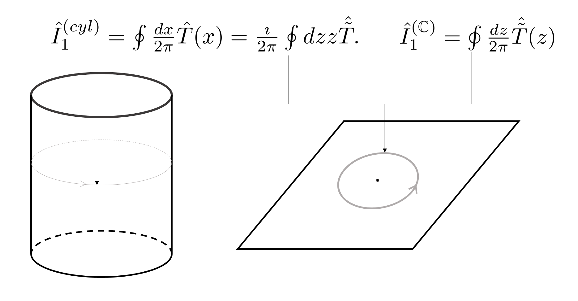
Figure 5: The contours of integration of the conserved quantities $\hat{I}_{1}^{(cyl)}$ and $\hat{I}_{1}^{(\mathds{C})}$. The contours of integration on the cylinder or the complex plane are indicated by arrows.

There is another way to obtain conserved quantities on the Riemann sphere, which yields different commuting quantities. Note that the proof that $\hat{I}^{(cyl)}_{2k+1}$ are commuting quantities relies only on the form of the commutation relations and on the fact that the integration contour, which defines the conserved quantity, is closed. This means that if we take the quantities in $I^{(cyl)}_{2k+1}$ and replace $dx$ by $dz,$ $\hat{T}$ by $\hat{\tilde{T}}$ and the integration contour around the cylinder by a closed contour in the complex plane surrounding the origin, we will get a mutually commuting set of quantities. We denote these conserved quantities by $\hat{I}_{2k+1}^{(\mathds{C})}$. This procedure is demonstrated in Fig. 5.

As mentioned above, the mutual eigenvalues of the commuting operators $\hat{I}_{2k+1}^{(cyl)}$ are the primary fields and descendants of conformal field theory. To find possible spectra and the properties of these eigenstates, one uses the representation theory of the Virasoro algebra, Eq. (6.29). We shall find opportunity in the next section to quote some results from this representation theory, but we will not review it here.

The diagonalization of $\hat{I}^{(\mathds{C})}_{2k+1}$ follows a different route. The reason for the different approach in comparison to $\hat{I}^{(cyl)}_{2k+1}$ is the fact that while $\hat{I}^{(cyl)}_{2k+1}$ are scale invariant, the operator $\hat{I}^{(\mathds{C})}_{2k+1}$ scale as $L^{-(1+2k)}$, where $L$ is sum large scale cut-off. For example, if we think of $\mathds{C}$ as the cylinder of radius $L$ in the limit $L\to\infty$, we expect that eigenvalue of $\hat{I}^{(\mathds{C})}_{1}$ to scale to zero in the limit $L\to\infty$ as $L^{-1}$, while $\hat{I}_{1}^{(cyl)}$ becomes a universal number independent of $L$ in the limit. The latter behavior (relating to $\hat{I}_{1}^{(cyl)}$) is more tractable using representation theory than the former behavior (relating to $\hat{I}_{1}^{(\mathds{C})}$). To diagonalize $\hat{I}_{1}^{(\mathds{C})}$, one rather puts the system on a cylinder of radius $L$ (to provide a cutoff) and solves the problem using the Bethe ansatz[37, 38, 39]. Indeed, treating the complex plane as a cylinder with the radius sent to infinity, the method of the quantum separation of variables discussed in section 6.1, produces the set of states, which simultaneously diagonalizes the quantum Hamiltonians $\hat{I}^{(\mathds{C})}_{1}$.

Regardless of how the two bases, which diagonalize the two commuting sets $\hat{I}^{(cyl)}_{2k+1},$ $\hat{I}^{(\mathds{C})}_{2k+1}$, are found, one may consider the expansion of a basis vector belonging to one set, in terms of the basis vectors belonging to the other. These objects, called form factors, are the main object we wish to introduce in this section. They hold special importance for the message this paper wishes to convey, as we shall argue in the next section that the modulus square of such form factors are an appealing candidate to describe the statistics of the Hele-Shaw interface and in particular may hold the key to analytically obtaining the fractal properties of the interface, including the fractal dimension.

To be able to more precisely introduce the form factors, let us first note that $\hat{I}^{(cyl)}_{2k+1}$ are usually diagonalized in terms operators, rather than directly by states, the two points of view being equivalent due to the operator-state correspondence of conformal field theory. One finds operators, $\hat{\Phi}(z),$ such that:

$$[\hat{I}^{(cyl)}_{2k+1},\hat{\Phi}(0)]=\tilde{\Delta}_{2k+1}\hat{\Phi}(0).$$ (6.38)

In addition, a vacuum, $|0\rangle$ is defined as a special highest weight state. Namely, this state satisfies:

$$\hat{L}_{n}|0\rangle=0,$$ (6.39)

for $n\geq-1$. An eigenstate of $I^{(cyl)}_{1}=L_{0}-\frac{c}{24}$ with eigenvalue $\tilde{\Delta}_{1}=\Delta_{1}-\frac{c}{24}$,can thus be written as:

$$\hat{\Phi}(0)|0\rangle.$$ (6.40)

The $z$ dependence of $\hat{\Phi}(z)$ is defined by:

$$[\hat{I}_{1}^{(\mathds{C})},\hat{\Phi}(z)]=\partial_{z}\hat{\Phi}(z),$$ (6.41)

which may be more familiar when one realizes $I_{1}^{(\mathds{C})}=L_{-1}$. In Addition, it can easily be show, based on Eqs. (6.28), (6.38) and the Baker-Campbell-Hausdorff lema, that the following relation holds:

$$e^{\imath\theta\oint z\hat{\tilde{T}}(z)}\hat{\Phi}(z_{0})e^{-\imath\theta\oint z\hat{\tilde{T}}(z)}=e^{\imath\Delta_{1}\theta}\hat{\Phi}(z_{0}e^{\imath\theta}).$$ (6.42)

As for the eigenstates of $\hat{I}_{2k+1}^{(\mathds{C})}$, these are obtained by quantizing the Korteweg-de Vries problem, as described in section 6.1. In that section it was shown that the separated variables of multi-phase solutions of classical Korteweg-de Vries become separated quantum operators. The eigenstates so obtained are then in one to one correspondence with multi-phase solutions of Korteweg-de Vries, which may be labelled by the hyper-elliptic surface $\mathcal{A}.$ We thus denote such eigenstates by $|\mathcal{A}\rangle$. In particular:

$$\hat{I}^{(\mathds{C})}_{2k+1}|\mathcal{A}\rangle=H_{2k+1}(\mathcal{A})|\mathcal{A}\rangle$$ (6.43)

We may now introduce the form factor. This is given by:

$$\langle\mathcal{A}|\hat{\Phi}(z)|0\rangle.$$ (6.44)

The form factors have had an important role in the study of integrable field theories, and a full understanding of them, would allow also for a full understanding of the integrable field theory beyond the spectrum. Important advances in this direction have been made by F. Smirnov (see [40] and references therein) and others (r.g., Refrs. [41, 42]) . How these objects stands in relations to the quantum Korteweg-de Vries and its semiclassical limit are described in Refrs. [43, 44, 45, 46].

The importance of the form factors lies in the fact that the set of states, $|\mathcal{A}\rangle,$ is, by definition, a complete basis and as such one can write a resolution of the identity as:

$$\mathds{1}=\oint|\mathcal{A}\rangle\langle\mathcal{A}|d\mathcal{A}.$$ (6.45)

The form factors then appear naturally when one inserts the resolution of the identity into correlators of the fields $\hat{\Phi}$. We must note, however, that in (6.45), the measure $d\mathcal{A}$ must be specified. In addition, it is not clear that the set of states described by the quasi periodic solutions, to which $\mathcal{A}$ serves as a label, are complete. Thus, it should be assumed that in (6.45), the label $\mathcal{A}$ may have to be generalized to go beyond labelling hyper-elliptic Riemann surface. We shall, however, in the sequel, be interested mainly in the semi-classical interpretation of Eqs. (6.45,6.44) and in a context where such distinctions are less crucial.

7 Quantum-Classical Distribution

We shall now discuss some properties of a certain sesquilinear of the form factor in Eq. (6.44). These properties will eventually clarify the reason for proposing a possible connection with the probability distribution $P(\mathcal{A})$. To do so, we need first to consider a semiclassical version of the form factor. We imagine taking a wave packet of quantum states such that the packet saturates the Heisenberg uncertainty bound and denote the packet by $|\mathcal{A}\!\!\succ,$ and define the object:

$$p(\mathcal{A})=\prec\!\!0|\hat{\Phi}(0)|\mathcal{A}\!\!\succ\prec\!\!\mathcal{A}|\hat{\Phi}(0)|0\!\!\succ.$$ (7.1)

Here we allow to take for the state $\prec\!\!0|\hat{\Phi}(0)$ some semiclassical approximation, and thus denote it as $\prec\!\!0|\hat{\Phi}(0)$ rather than as $\langle 0|\hat{\Phi}(0)$.

7.1 Time-Translation and Scale Invariance

We would like to show that $p(\mathcal{A})$ is time translation invariant, just as $P(\mathcal{A})$, Eq. (1.3). First, from (6.43) we have for any sufficiently well behaved generic (namely, one that cannot be written as a linear combination of $\hat{I}_{2k+1}^{(\mathds{C})}$) operator, $\hat{O}$:

$$\lim_{\delta\to 0}e^{-\imath\Delta t\left(\hat{I}_{1}^{(\mathds{C})}+\delta\hat{O}\right)}|\mathcal{A}\rangle=e^{-\imath\Delta tH_{1}(\mathcal{A})}|\mathcal{A}\rangle.$$ (7.2)

Now semiclassically, and by using the Whitham method, which states that any perturbation will lead, in zeroth order, to the Whitham evolution, we may write:

$$\lim_{\delta\to 0}e^{-\imath\Delta t\left(\hat{I}_{1}^{(\mathds{C})}+\delta\hat{O}\right)}|\mathcal{A}\rangle\sim|\mathcal{A}^{\Delta t}\!\!\succ$$ (7.3)

Assuming that the object:

$$\langle 0|\hat{\Phi}(0)e^{-\imath\Delta t\left(\hat{I}_{1}^{(\mathds{C})}+\delta\hat{O}\right)}|\mathcal{A}\rangle$$ (7.4)

is smooth as $\delta\to 0,$ we obtain, by employing (7.2):

$$\lim_{\delta\to 0}\prec\!\!0|\hat{\Phi}(0)e^{-\imath\Delta t\left(\hat{I}_{1}^{(\mathds{C})}+\delta\hat{O}\right)}|\mathcal{A}\!\!\succ\prec\!\!\mathcal{A}|e^{\imath\Delta t\left(\hat{I}_{1}^{(\mathds{C})}+\delta\hat{O}\right)}\hat{\Phi}(0)|0\!\!\succ=p(\mathcal{A}),$$ (7.5)

which when compared with Eq. (7.3) gives:

$$p(\mathcal{A})=p(\mathcal{A}^{\Delta t}).$$ (7.6)

To show that $p$ also has the requisite scale invariance property, we must first consider the correlation function:

$$\langle 0|\hat{\Phi}(0)\hat{\Phi}(z)|0\rangle=\frac{C}{z^{2\Delta_{1}}},$$ (7.7)

where

$$C=\langle 0|\hat{\Phi}(0)\hat{\Phi}(1)|0\rangle.$$ (7.8)

this equality being easily obtained by making use of (6.42). On the other hand by employing the resolution of identity, Eq. (6.45), one obtains:

$$\langle 0|\hat{\Phi}(0)\hat{\Phi}(z)|0\rangle=\int\langle 0|\hat{\Phi}(0)|\mathcal{A}\rangle\langle\mathcal{A}|\hat{\Phi}(z)|0\rangle d\mathcal{A}.$$ (7.9)

This equation may be written through $p(\mathcal{A})$:

$$\langle 0|\hat{\Phi}(0)\hat{\Phi}(z)|0\rangle=\int p(\mathcal{A})e^{-zH_{1}(\mathcal{A})}d\mathcal{A},$$ (7.10)

which when combined with (7.7) yields:

$$p(\mathcal{A})d\mathcal{A}\sim d\left(H_{1}(\mathcal{A})\right)^{2\Delta_{1}},$$ (7.11)

where $H_{1}(\mathcal{A})\$ is the dispersionless Korteweg-de Vries first Hamiltonian, Eq. (5.12), for the Riemann surface $\mathcal{A}$. If we interpret the algebraic Riemann by means of the Hele-Shaw interface, we have the relation $H_{1}(\mathcal{A})\sim\sqrt{R}$ such that we may write:

$$p(R)dR\sim dR^{\Delta_{1}}.$$ (7.12)

We also make a note on the measure, $d\mathcal{A}$. We should demand that this measure is time translation invariant. We believe that this is indeed the case, as the measure of integration for the semiclassical wave-function is often assumed to be the Liouville measure[43, 44, 46]. This measure is time-translation invariant, by a well-known theorem. The fact that it is time translation invariant with respect to the Whitham evolution, may abe surmised by noting that Whitham evolution is the zeroth order limit in any well-behaved perturbation. In the zeroth order the time translation invariance of the metric must be recovered, and so the measure must be invariant with respect to the Whitham evolution as well.

7.2 Some Results from Virasoro Representation Theory

Figure 6: The spectrum of dimensions, $D$, for the first non-trivial unitary minimal models. Only dimensions between $1$ and $2$ are shown. Empty circles represent first descendent of primary fields (namely, fields with dimensions $D=\Delta^{(r,s)}+1),$ higher descendants do not have fractal dimensions between $1$ and $2$, filled circles represent primary fields (namely, fields with dimensions $D=\Delta^{(r,s)}$). The minimal unitary model with $m=6,$ corresponding to $c=6/7$, contains a field with dimension $12/7.$ This field is the $(5,3)$ field in the Kac classification. The first descendent of the Kac $(5,4)$ field has the same dimension. Only a few fields, and fewer primaries, are above the line $D=3/2$ corresponding to Kesten’s bound [47], $D\geq 3/2.$

Both the proposed time translation invariance and the scale invariance of $p(\mathcal{A}),$ Eqs. (7.6) and (7.12), compare well, with the properties expected from the Hele-Shaw probability function Eqs. (1.3) and (1.5) , respectively, if we identify the $\hat{I}_{1}^{(cyl)}$ eigenvalue associated with $\hat{\Phi}$, namely, $\Delta_{1},$ with the fractal dimension, $D$. It turns out, that the representation theory for the Virasoro algebra (the algebra given in Eq. (6.29)), gives a discrete spectrum (again under some assumptions) for the possible values of $\Delta_{1}$, and hence for the fractal dimension $D$.

At this point, it is perhaps advisable to reiterate that a more satisfactory connection between Laplacian growth and the representation theory of conformal field theory, would start from the two dimensional Toda lattice hierarchy rather than the Korteweg-de Vries hierarchy. As it stands, the relation between the Korteweg-de Vries limit of Laplacian growth and conformal field theory may not be satisfactory in order to make even conjectural statements. Thus, the purpose of the current exercise linking the fractal dimension, $D$, to the eigenvalue, $\Delta_{1},$ in conformal field theory, is give the gist of how the computation may work within a framework of more comprehensive theory.

After these words of caution, let us remind the reader that the representation theory of the Virasoro algebra, Eq. (6.29), admits representations which depend on $c$, which appears in (6.29) on the right hand side. Among those representation there are distinguished values of $c$, at which the especially simple representations exist, the field theories at those values of $c$ are called minimal models. These representations are simple in the fact that finite number of fields $\hat{\Phi}$ satisfying condition (6.38) can be chosen that generate the entire representation. These are called primary fields and are labelled by two number $r,s$. We write $\hat{\Phi}_{r,s}$ for such a field. We concentrate here on such representations which are unitary. For unitary representations, the possible values of $c$ are given by:

$$c=1-\frac{6}{m(m+1)},$$ (7.13)

where $m$ is an integer larger or equal to $3$, $m\geq 3$. Within these theories and for the operators $\hat{\Phi}_{r,s},$ the labels $r$ and $s$ can take the values $1\leq r<m$, $1\leq s\leq r$. The value of $\Delta_{1}$ for $\hat{\Phi}_{r,s}$, which we denote by $\Delta_{1}^{(r,s)}$, is given by:

$$\Delta_{1}^{(r,s)}=\frac{\left[(m+1)r-ms\right]^{2}-1}{4m(m+1)}.$$ (7.14)

Other solutions of (6.38) have a dimension $\Delta_{1}$ which may be larger by an integer, $\Delta_{1}=\Delta_{1}^{(r,s)}+n$, for some $n\geq 0$.

We have focused on the unitary models, since they seem to have the kind of properties which are needed to have a consistent description of the modulus square of the form factors as the Laplacian growth probability distribution. But of course, this statement must be taken with a grain of salt. At any rate, one can focus on these models and see whether the fractal dimension $D$ which is observed in Laplacian growth [1, 2], $D=1.71\pm 0.3,$ is reproduced in this approach as $D=\Delta_{1}^{(r,s)}+n$, for some admissible values $n$, $r$ and $s$. The observed fractal dimension have long been recognized as being equal to $D=12/7,$ within the accuracy of the observation. As shown in Fig. 6, such a fractal dimension appears at $m=6$ for $r=5$, $s=3$ and $n=0$ and for $r=5$, $s=4$ and $n=1$.

Many other fractal dimension, $D,$ can be found for, say, the first four unitary models, $3\leq m\leq 6.$ However, given that the fractal dimension of cluster embedded in two dimensions must be between $1$ and $2$, and moreover given Kesten’s work who showed that $3/2\leq D\leq 2$, only a few possible fractal dimension appear for the first four unitary minimal models, and $D=12/7$ may be found among their numbers. We should note that Kesten’s bound was found for the closely related process of diffusion limited aggregation[48], believed to be in the universality class of Laplacian growth [1]. We should also note that the number of fractal dimensions respecting the known bounds, increases rapidly as $m$ increases, such that without further insight into how to determine the correct conformal field theory, labelled by $c$, from which to take the fractal dimension, the approach will not yield unambiguous results, this of course assuming the validity of the approach in the first place.

8 Conclusion

We have presented a possible connection between Laplacian growth and conformal field theory, which relies on the classical and quantum integrability of the problems, respectively, after reviewing some necessary material regarding the classical integrability of the Laplacian growth problem and the quantum inverse scattering method applied to conformal field theory and the quantum Korteweg-de Vries equation. It is perhaps advisable to stress again the tentative nature of the proposed connection. At the same time, it may be reasonably said that the proposed connection seems to be offer an interesting paradigm for how non-equilibrium integrable systems may be treated analytically. Namely, that a sort of spectral expansion of field theory operators may provide the probability density for a non-equilibrium system. The prospect of such an approach is appealing because it allows to deviate from the more common analytic device of proposing Gibbs or Gibbs-like measures for the solution of non-equilibrium problems (for example, in problems of large deviations in which probability densities can be understood and computed as the exponent of some non-equilibrium action), while allowing for progress within an analytic approach.

Appendix A The Baker-Akhiezer Function: Existence and Explicit Form

We give here an expression Baker-Akhiezer functions defined on some Schottky double. To do so it is necessary to describe the Schottky double by the ‘Jacobi variety’. This description is very familiar in the case of a genus $1$ surface. In that case There are two interfaces and two cycles $a$, $b$. (see Fig. (3)). a genus $1$ surface has the topology of a torus and a torus is well known to be representable in terms of a rectangle with opposite sides identified. This latter is the Jacobi variety for a genus $1$ surface. The extension of this two higher genus surfaces, when there more than two interfaces, is described below. The construction is then used in order to write an explicit formula for the Baker-Akhiezer function on the Schottky double.

A genus $g$ surface admits $g$ independent holomorphic differentials. A natural basis for such differentials is given by $\zeta_{i}$ required to be holomorphic one-forms satisfying:

$$\oint_{a_{k}}\zeta_{j}=\delta_{jk}.$$ (A.1)

Let us consider the Abel map[49, 22, 50] $\vec{u}(\bm{z}):\mathcal{D}\longrightarrow\mathds{C}^{g}/(\mathds{Z}^{g}+\bm{B}\mathds{Z}^{g}),$ where

$$\bm{B}_{kj}=\oint_{b_{k}}\zeta_{j}.$$ (A.2)

The Abel map is defined by:

$$u_{j}(\bm{z})=\int^{\bm{z}}_{\bm{z}_{0}}\zeta_{j}\mod\vec{v},\quad\vec{v}\in\mathds{Z}^{g}+\bm{B}\mathds{Z}^{g},$$ (A.3)

where $\bm{z}_{0}$ is some point on the Schottky double satisfying $\tau(\bm{z})=\bm{z}.$ Namely, $\vec{u}(\bm{z})$ is a vector whose $j$ element is $\int^{\bm{z}}\zeta_{j}$, whereby the freedom in drawing the contour of integration to surround $m$ times around cycle $a_{k}$ and $n$ times around cycle $b_{l}$ leads to an additive ambiguity in the value of $\vec{u}$ of the form $m\hat{e}_{k}+n\bm{B}\hat{e}_{l}.$ To remove this ambiguity $\vec{u}(\bm{z})$ is considered to take values in the Jacobian $\mathds{C}^{g}/(\mathds{Z}^{g}+\bm{B}\mathds{Z}^{g})$. For $g\geq 1$ the image of the Abel map is a two dimensional surface within the Jacobian.

The matrix $\bm{B}$ turns out to be symmetric and, because of the existence of an anti-holomorphic involution, $\bm{B}$ is purely imaginary. Furthermore, the matrix $\bm{B}$ is positive definite. This allows to define the Riemann theta as follows:

$$\theta(\vec{u})=\sum_{\vec{n}\in\mathds{Z}^{g}}\exp 2\pi\imath\left[\vec{n}\cdot\vec{u}+\frac{\vec{n}^{t}\bm{B}\vec{n}}{2}\right].$$ (A.4)

The Riemann Theta function is quasi-periodic on the Jacobian:

$$\theta(\vec{u}+\hat{e}_{k})=\theta(\vec{u}),\quad\theta(\vec{u}+\bm{B}\hat{e}_{j})=e^{-\pi\imath B_{jj}-2\pi\imath u_{j}}\theta(\vec{u}).$$ (A.5)

The function itself is, thus, not single valued on the Jacobian. Nevertheless, it may be used to construct all single valued holomorphic functions on the Riemann surface by taking proper combinations of it. For example, the logarithmic derivative of $\theta$ is already single valued.

The Baker-Akhiezer function can be written in terms of the Riemann theta function, as well. However, to write the explicit expression, we shall first need, for each $k$ to define two $g$-dimensional vectors $\vec{\omega}^{a}_{k},\vec{\omega}^{b}_{k}$, as follows :

$$\left(\vec{\omega}_{k}^{a}\right)_{j}=\imath\oint_{a_{j}}dH_{k},\quad\left(\vec{\omega}_{k}^{b}\right)_{j}=-\imath\oint_{b_{j}}dH_{k}.$$ (A.6)

In addition, let us define a set of points $\bm{\gamma}^{\pm}_{j}$ as a set of $g$ points on the Schottky double, such that $\bm{\gamma}^{+}_{j}=\tau(\bm{\gamma}_{i}^{-}),$ and such that there exist a differential $d\Omega$ with first order poles at $\infty_{\pm}$ with residues $\pm 1$, respectively, and with zeros at the points $\bm{\gamma}_{j}^{+}$ and $\bm{\gamma}_{j}^{-}$. We let $\vec{u}_{(i)}^{\pm}=\vec{u}(\bm{\gamma}^{\pm}_{i})$, respectively.

We denote from here on

$$H_{0}=H/2,\quad t_{0}=t=n.$$ (A.7)

The explicit expression for the Baker Akhiezer function, $\psi^{+}$, and a function $\psi^{-}$, which may be treated as its adjoint, reads as follows:

$$\psi_{n}^{\pm}(\bm{z})=e^{\pm\sum_{k\geq 0}t_{k}{H}_{k}+\bar{t}_{k}\bar{{H}}_{k}}\Phi^{\pm}\left(\left.\sum_{k}{\rm Re}\left[t_{k}(\bm{B}\vec{\omega}_{k}^{a}+\vec{\omega}_{k}^{b})\right]\right|\vec{u}(\bm{z})\right).$$ (A.8)

where $\Phi^{\pm}(\vec{w}|\vec{u})$ is a function of two complex $g$-dimensional vectors, $\vec{w}$ and $\vec{u}$. The function $\Phi^{\pm}$ takes the following explicit form:

$$\Phi^{\pm}(\vec{w}|\vec{u})=A^{\pm}(\vec{w})e^{\pm 2\pi\imath\vec{u}\cdot\bm{B}^{-1}{\rm Im}(\vec{w})}\frac{\theta\left(\vec{u}\pm\vec{w}-\sum_{i}\vec{u}_{(i)}^{\pm}+\vec{K}\right)}{\theta(\vec{u}-\sum_{i}\vec{u}_{(i)}^{\pm}+\vec{K})},$$ (A.9)

where $\vec{K}$ is the vector of Riemann constants, which is given by:

$$K_{i}=\frac{1+B_{ii}}{2}-\sum_{j\neq i}\oint_{a_{j}}u_{i}\zeta_{j}.$$ (A.10)

Expression (A.8) is single valued on the Riemann surface even though, as noted before, the Hamiltonians are multi-valued function. In fact, the explicit form for the Baker-Akhiezer function is constructed such as the quasi-periodicity of the Riemann theta function exactly cancels the quasi periodicity of the exponent of the Hamiltonians as they appear in (A.8).

The amplitudes, $A^{\pm}$, are, for now, arbitrary. The fact that the Baker-Akhiezer function defined in Eq. (A.8) indeed solves the spectral problem, Eq. (4.21), will be shown in appendix B based on the following analytic properties that this functions obeys:

• As $z\to\infty_{\uparrow}$, the Baker-Akhiezer functions have following expansion:

  $$\psi^{\pm}_{n}=z^{\pm n}e^{\pm\sum_{k>0}t_{k}z^{k}}\sum_{j\geq 0}\frac{\xi^{\pm,\uparrow}_{jn}}{z^{k}},$$ (A.11)

  while as $z\to\infty_{\downarrow}$, the Baker Akhiezer functions have the following expansion

  $$\psi^{\pm}_{n}=\bar{z}^{\mp n}e^{\mp\sum_{k>0}\bar{t}_{k}{\bar{z}^{k}}}\sum_{j\geq 0}\frac{\xi^{\pm,\downarrow}_{jn}}{\bar{z}^{j}}.$$ (A.12)

  The parameters $\xi^{\pm,\uparrow/\downarrow}_{jn}$ are functions of the times, $t_{k}$, $\bar{t}_{k}$.

• The functions $\psi_{n}^{\pm}(z)$ have poles at the points $\bm{\gamma}_{j}^{\pm}$, respectively. This fact is based the Riemann theta function participating in the definition of $\Phi^{\pm}$ has zeros at those points[49, 50, 22].

• The amplitudes $A^{\pm}$ may be chosen such that the Baker-Akhiezer functions are normalized by requiring $\xi^{+,\uparrow}_{0n}$ to be real and positive along with the following condition

  $$\xi_{0n}^{+,\uparrow}=\frac{1}{\xi_{0n}^{-,\uparrow}}=\frac{1}{\xi_{0n}^{+,\downarrow}}.$$ (A.13)

These analytic properties can be ascertained from the explicit form of the Baker-Akhiezer function, Eq. (A.8).

It is important to note that the Riemann theta function has $g$ zeros, and thus the Baker-Akhiezer function vanishes at $g$ points on the Riemann surface. As discussed in Ref. [33] and reviewed in section 5.3, the $z$ coordinate of the points on the Riemann at which the Baker-Akhiezer function vanishes, can be considered as set of $g$ dynamical variables. One may take the Bloch multiplier associated with the Baker-Akhiezer function on the opposite sheet of the Schottky double as another set of $g$ dynamical variables. Together we have $2g$ dynamical variables, which, as discussed in section 5.3 in the context of the Korteweg-de Vries equation, are separated variables .

Appendix B The Baker-Akhiezer Function: Definition and Properties

Assume a Schottky double, with anti-holomorphic involution, $\tau$. We assume that as $z\to\infty$, the function $\tau(z)$ may be expanded as $\tau(z)=z^{J}+O(z^{J-1}),$ for some positive integer, $J$, which one should assume to be large.

We have defined the Baker-Akhiezer function as a function satisfying (4.21). We need a somewhat more explicit and detailed definition of the spectral problem. We write this definition here as follows:

$$\sum_{m}L_{nm}\psi^{+}_{m}=z\psi^{+}_{n},\quad\sum_{m}\psi^{-}_{m}L_{mn}=z\psi^{-}_{n}$$ (B.1)

$$\sum_{m}L^{\dagger}_{nm}\psi^{+}_{m}=\overline{\tau(z)}\psi^{+}_{n},\quad\sum_{m}\overline{L_{nm}}\psi^{-}_{m}(z)=\overline{\tau(z)}\psi^{-}_{n}$$ (B.2)

$$\partial_{l}\psi^{+}_{n}=\sum_{m}L_{nm}^{(l)}\psi^{+}_{m},\quad\partial_{l}\psi^{-}_{n}=-\sum_{m}^{(l)}\psi^{-}_{m}L^{(l)}_{mn},$$ (B.3)

$$\bar{\partial}_{l}\psi^{+}_{n}=\sum_{m}L^{(l)\dagger}_{nm}\psi^{+}_{m},\quad\bar{\partial}_{l}\psi^{-}_{n}=-\sum_{m}\overline{L^{(l)}_{nm}}\psi^{-}_{m},$$ (B.4)

Equations (B.3), (B.4) should be understood as written on the front side, and may be analytically continued to the back side. Thus for example $z$ in (B.3) is to be replaced by $\tau(z)$ on the back side.

Given that the analytic conditions the Baker-Akhiezer functions obeys, detailed in appendix A, one may prove that these functions obey a list of properties enumerated below. The central item in the list is the fact that the Baker-Akhiezer function solves the Lax spectral problem. The properties enumerated as 1- 4 below may be treated as lemmas helping to prove this central fact, which itself is enumerated as property 5 below.

1. Uniqueness:
   A function $f^{\pm}_{n}$ satisfying the same conditions as $\psi^{\pm}_{n}$, Eqs. (A.11-A.13), is equal to $\psi^{\pm}_{n}$. A function $f^{\pm}_{n}$ satisfying the same conditions as $\psi^{\pm}_{n}$, except the normalization condition, Eq. (A.13), is proportional to $\psi^{\pm}_{n}.$

2. Orthonormality:

   $$\frac{1}{2\pi\imath}\oint_{\mathcal{C}}\psi^{-}_{n}(z)\psi^{+}_{m}(z)d\Omega=\delta_{n,m},$$ (B.5)

   where $d\Omega$ is a differential with first order poles at $\infty_{\pm}$ with residues $\pm 1$, respectively, and with zeros at the points $\bm{\gamma}_{j}^{+}$ and $\bm{\gamma}_{j}^{-}$. The differential is normalized such that its integral over any cycle is purely imaginary.

3. Completeness:
   Consider functions, $f^{\pm}$, on the Schottky double meromorphic everywhere except at $\infty_{\uparrow/\downarrow}$, where they have the expansions:

   $$f^{\pm}=\left\{\begin{array}[]{lr}z^{m^{\pm}_{\uparrow}}e^{\sum_{k>0}t_{k}z^{k}}\sum_{j\geq 0}C^{\pm,\uparrow}_{j}z^{-j},&z\to\infty_{\uparrow}\\ \bar{z}^{-m^{\pm}_{\downarrow}}e^{-\sum_{k>0}\bar{t}_{k}\bar{z}^{k}}\sum_{j\geq 0}C^{\pm,\downarrow}_{j}\bar{z}^{-j},&z\to\infty_{\downarrow}\end{array}\right.,$$ (B.8)

   with poles at $\bm{\gamma}_{i}^{\pm}$, respectively. The completeness property states that such functions are expandable in terms of Baker-Akhiezer functions. Namely, there exist coefficients $\alpha^{\pm}_{j}$ such that:

   $$f^{\pm}=\sum_{j=n_{1}^{\pm}}^{n_{2}^{\pm}}\alpha^{\pm}_{j}\psi^{\pm}_{j},$$ (B.9)

   where $n^{+}_{1}=m_{\downarrow}^{+},n^{-}_{1}=m^{-}_{\uparrow},n^{+}_{2}=m^{+}_{\uparrow},n_{2}^{-}=m_{\downarrow}^{-},$ respectively. The expansion (B.9) holds if $n_{2}^{+}\geq n_{1}^{+}$, otherwise $f^{+}=0$. Similarly, $f^{-}=0$ unless $n_{2}^{-}\geq n_{1}^{-}$.

4. Reflection:

   $$\overline{\psi_{n}^{+}(\tau(z))}=\psi_{n}^{-} (z),\quad\overline{\psi_{n}^{-}(\tau(z))}=\psi_{n}^{+}(z),$$ (B.10)

   $$-\overline{d\Omega(\tau(z))}={d\Omega}(z)$$ (B.11)

5. Spectral problem:
   The Baker-Akhiezer functions, $\psi_{n}^{+},$ are wave-functions associated with the Lax spectral problem. Namely, Eqs. (B.1-B.4) hold, with (4.7).

We now give brief, semi-rigorous ‘proofs’ of these properties
 Proof of 1.

If two such functions $\psi_{n}$ and $\tilde{\psi}_{n}$ exist, then their ratio $\frac{\psi_{n}}{\tilde{\psi}_{n}}$ is a meromorphic function which has zeros at the poles of $\tilde{\psi}_{n}$ and the zeros of $\psi_{n}$. The Riemann-Roch theorem[49, 50, 22] states that, generically, a function cannot be found with arbitrarily chosen positions for the zeros. Thus, the zeros and poles of $\tilde{\psi}$ and $\psi$ coincide, namely $\frac{\psi_{n}}{\tilde{\psi}_{n}}$ is entire on the compact Riemann surface, and thus $\frac{\psi_{n}}{\tilde{\psi}_{n}}=c,$ where $c$ is some constant independent on $z$. The normalization condition (A.13) fixes this constant to be $1$.
Proof of 2:

Consider the integrand $\psi^{+}_{n}(\{t^{\prime}_{k}\},z)\psi^{-}_{m}(\{t_{k}\},z)d\Omega$ has no singularities except at $\infty_{\uparrow/\downarrow}$ where it has the form $z^{(n-m)-1}\xi_{0}^{-,\uparrow}dz$ and $-z^{(m-n)-1}\xi_{0}^{+,\downarrow}dz$, respectively. If $n>m$ we may deform the contour of integration to surround $\infty_{\downarrow}$ and obtain the the integral is zero and if $n<m$ we may deform the contour of integration to surround $\infty_{-}$ with the same conclusion. If $n=m,$ we may deform the contour of integration to surround $\infty_{+}$ to obtain that the integral is given by $1$, by using Eq. (A.13). If for $n=m$ we deform the contour of integration around $\infty_{-}$ instead of around $\infty_{+}$ and apply the condition that the result must not depend on the choice of how to deform he contour, one obtains $\xi_{0n}^{-,\downarrow}=\frac{1}{\xi_{0n}^{+,\downarrow}}.$ The latter relation naturally joins the normalization condition Eq. (A.13), and so we record here the full normalization condition, which includes this relation, for future reference:

$$\xi_{0n}^{+,\uparrow}=\frac{1}{\xi_{0n}^{-,\uparrow}}=\frac{1}{\xi_{0n}^{+,\downarrow}}=\xi^{-,\downarrow}_{0,n}.$$ (B.12)

Proof of 3:

Let us focus on $f^{+}$, only. The proof with regards to $f^{-}$ goes along the same lines, so we shall omit it.

Let us assume first that $m^{+}_{\uparrow}\geq m_{\downarrow}^{+}$. Given the expansion of $\psi_{j}^{+}$ around $\infty_{\uparrow}$, Eq. (A.11), one sees that one may cancel the coefficients $C^{+,\uparrow}_{j}$ in (B.8), one by one for $j=m^{+}_{\uparrow},\dots,m_{\downarrow}^{+}+1$ by adding to $f^{+}$ a linear combination of $\psi^{+}_{j},$ and this without affecting the leading order behavior around $\infty_{\downarrow}$. More formally, there exists a set of numbers $\{\alpha_{j}^{+}\}_{j=m_{\downarrow}^{+}+1}^{m_{\uparrow}^{+}}$ such that the following expansion for the function $\tilde{\psi}\equiv f^{+}-\sum^{m^{+}_{\uparrow}}_{j=m^{+}_{\downarrow}+1}\alpha_{j}^{+}\psi^{+}_{j}$ holds around $\infty_{\uparrow/\downarrow}$:

$$\tilde{\psi}=\left\{\begin{array}[]{lr}z^{m_{\downarrow}^{+}}e^{\sum t_{k}z^{k}}(c_{\uparrow}+O(1/z))&z\to\infty_{\uparrow}\\ \bar{z}^{-m_{\downarrow}^{+}}e^{-\sum\bar{t}_{k}\bar{z}^{k}}(c_{\downarrow}+O(1/\bar{z}))&z\to\infty_{\downarrow}\end{array}\right.,$$ (B.15)

for some $c_{\uparrow}$ and $c_{\downarrow}$. Since $\tilde{\psi}$ satisfies all the analytic requirements defining the Baker-Akhiezer function $\psi^{+}_{m_{\downarrow}^{+}},$ except perhaps the normalization condition, it follows from uniqueness (property 1 above), that $\tilde{\psi}$ must be proportional to $\psi^{+}_{m_{\downarrow}^{+}}.$ Let us denote the constant of proportionality by $\alpha^{+}_{m_{\downarrow}^{+}}$ and write

$$\tilde{\psi}=f^{+}-\sum^{m^{+}_{\uparrow}}_{j=m^{+}_{\downarrow}+1}\alpha_{j}^{+}\psi^{+}_{j}=\alpha_{m^{+}_{\downarrow}}^{+}\psi^{+}_{m_{\downarrow}^{+}},$$

from which (B.9) follows immediately for $f^{+}$ and with $n_{1}^{+}=m^{+}_{\downarrow}$ and $n_{2}^{+}=m^{+}_{\uparrow}$.

If $m^{+}_{\uparrow}<m_{\downarrow}^{+}$, then it follows that $f^{+}$ obeys all the analytic conditions required of $\psi^{+}_{m_{\downarrow}^{+}}$, except the normalization condition. Indeed, the expansion of $f^{+}$ around $\infty_{\downarrow}$ is given by the form on the right hand side of Eq. (A.12), while the expansion around $\infty_{\uparrow}$, is given by the right hand side of Eq. (A.11) with $\xi^{+,\uparrow}_{0m_{\downarrow}}=0$, and the existence of a normalized Baker-Akhiezer function. Thus, due to uniqueness, $f^{+}=\alpha\psi^{+}_{m_{\downarrow}^{+}}$, for some $\alpha$. The fact that $\alpha=0$ follows from $\xi^{+,\uparrow}_{0m_{\downarrow}}=0$, showing that if $n_{2}^{+}<n_{1}^{+},$ then $f^{+}=0$.
Proof of 4:

If one compares the asymptotic expansion of $\psi^{-},$ given in (A.11),(A.12) with the expansion of $\overline{\psi^{+}}(\overline{\tau(z)})$ one sees that they match, based on (B.12), and the fact that $p(z)$ maps $\infty_{\uparrow/\downarrow}$ to $\infty_{\downarrow/\uparrow}$, respectively. The location of the poles match as well. The uniqueness of the Baker-Akhiezer function, then dictates that the two functions must be equal, proving the first equality in (B.10). The proof of the second equality follows much the same lines.

The equality, (B.11), may be proved by comparing the analytic properties of the left and right hand sides. The poles and residues are the same. The $a$ and $b$ cycle integrals are purely imaginary on both right and left hand side. Two differentials having the same singularities normalized to have imaginary periods over any cycle are equal, since their difference is a holomorphic differential with imaginary periods. The latter is necessarily zero, since the requirement of zero imaginary period represents $2g$ real linear constraints on the $2g$ dimensional space of holomorphic differentials (viewed as a vector space over $\mathds{R}$).
Proof of 5:

The analytic function on the Schottky double, which on the front side is given by $z$ is given on the back side by $\tau(z)$, which as $z\to\infty_{\downarrow}$ has the expansion $\tau(z)=\bar{z}^{J}+O(\bar{z}^{J-1})$, thus the front-side function $z\psi_{n}^{+}$, when analytically continued to the back side, has the expansion:

$$z\psi_{n}^{+}=\left\{\begin{array}[]{lr}z^{n+1}e^{\sum t_{k}z^{k}}(C_{\uparrow}+O(1/z))&z\to\infty_{\uparrow}\\ \bar{z}^{-(n-J)}e^{-\sum\bar{t}_{k}\bar{z}^{k}}(C_{\downarrow}+O(1/\bar{z}))&z\to\infty_{\downarrow}\end{array}\right..$$ (B.18)

By the completeness property (3 above), we obtain that there exist coefficients $L_{nj}$, which are non-zero for $j=n-J,\dots,n+1$ and vanish otherwise, such that:

$$z\psi_{n}^{+}=\sum_{j=n-J}^{n+1}L_{nj}\psi^{+}_{j}.$$ (B.19)

This defines the matrix $L$ with the property (4.3) and proves the first equality in (B.1). By orthonormality (Eq. (B.5)), we have:

$$L_{nj}=\frac{1}{2\pi\imath}\oint_{\mathcal{C}}\psi^{-}_{j}z\psi^{+}_{n}d\Omega.$$ (B.20)

Similarly, considering $z\psi^{-}$, the completeness property shows:

$$z\psi^{-}_{n}=\sum^{n+J}_{j=n-1}\tilde{L}_{nj}\psi^{-}_{j},$$ (B.21)

and orthonormality gives:

$$\tilde{L}_{nj}=\frac{1}{2\pi\imath}\oint_{\mathcal{C}}\psi^{-}_{n}z\psi^{+}_{j}d\Omega=L_{jn},$$ (B.22)

such that $\tilde{L}=L^{t}$, and the second equality in (B.1) is obtained.

The same considerations allow one to write:

$$\overline{\tau(z)}\psi^{+}_{n}=\sum_{j=n-1}^{n+J}\tilde{\tilde{L}}_{nj}\psi^{+}_{j},$$ (B.23)

with

$$\tilde{\tilde{L}}_{nj}=\frac{1}{2\pi\imath}\oint\psi^{-}_{j}\overline{\tau(z)}\psi^{+}_{n}d\Omega$$ (B.24)

We note that the analytic continuation of the front-side function $\overline{\tau(z)}$ is equal to $\bar{z}$ on $\mathcal{C}$. Thus taking the complex conjugate of this equation and, in addition, using the reflection property (4), we obtain:

$$\overline{\tilde{\tilde{L}}_{nj}}=\frac{1}{2\pi\imath}\oint\psi^{+}_{j}z\psi^{-}_{n}d\Omega=L_{jn},$$ (B.25)

such that $\tilde{\tilde{L}}=L^{\dagger}$. Proving the first equation in (B.2). The proof of the second equation follows the same lines and we omit it.

To prove the first equation in (B.3) we examine the expansion of $\partial_{l}\psi^{+}_{n}$ around $\infty_{\uparrow/\downarrow}$:

$$\partial_{l}\psi^{+}_{n}=\left\{\begin{array}[]{lr}z^{n+l}e^{\sum t_{k}z^{k}}\left(\sum_{j=0}^{l-1}\frac{\xi_{jn}^{+,\uparrow}}{z^{j}}+\frac{\xi_{jn}^{+,\uparrow}+\partial_{l}\xi^{+,\uparrow}_{0n}}{z^{l}}+\dots\right)&z\to\infty_{\uparrow}\\ \bar{z}^{-n}e^{-\sum\bar{t}_{k}\bar{z}^{k}}(\partial_{l}\xi_{0n}^{+,\uparrow}+\dots)&z\to\infty_{\downarrow}\end{array}\right..$$ (B.28)

Thus we have from completeness:

$$\partial_{l}\psi^{+}_{n}-\psi^{+}_{n}\frac{\partial_{l}{\xi^{+,\downarrow}_{0n}}}{{\xi^{+,\downarrow}_{0n}}}=\sum_{j=n+1}^{n+l}L^{(l)}_{nj}\psi^{+}_{j},$$ (B.29)

which entails:

$$\partial_{l}\psi^{+}_{n}=\sum_{j=n}^{n+l}L^{(l)}_{nj}\psi^{+}_{j},$$ (B.30)

with

$$L^{(l)}_{nj}=\left\{\begin{array}[]{lr}\frac{1}{2\pi\imath}\oint_{\mathcal{C}}\psi^{-}_{j}\partial_{l}\psi^{+}_{n}&n+l\geq j\geq n\\ \frac{\partial_{l}{\xi^{+,\downarrow}_{0n}}}{{\xi^{+,\downarrow}_{0n}}}&j=n\\ 0&{\rm otherwise}\end{array}\right..$$ (B.34)

To obtain the expression (4.7), for $L^{(l)},$ compare (B.28) with the expansion of $z^{l}\psi^{+}_{n}$ to obtain:

$$\partial_{l}\psi^{+}_{n}-z^{l}\psi^{+}_{n}-\psi^{+}_{n}\frac{\partial_{l}{\xi^{+,\uparrow}_{0n}}}{{\xi^{+,\uparrow}_{0n}}}=\sum_{j=n-J}^{n-1}\alpha_{j}\psi^{+}_{j},$$ (B.35)

for appropriately chosen $\alpha_{j}$. Applying the orthonormality property, Eq. (B.5), to this equation, while taking into account Eq. (B.34), one obtains:

$$L^{(l)}_{nj}=\left\{\begin{array}[]{lr}\frac{1}{2\pi\imath}\oint_{\mathcal{C}}\psi^{-}_{j}z^{l}\psi^{+}_{n}&n+l\geq j\geq n\\ \frac{\partial_{l}{\xi^{+,\uparrow}_{0n}}}{{\xi^{+,\uparrow}_{0n}}}+\frac{1}{2\pi\imath}\oint_{\mathcal{C}}\psi^{-}_{n}z^{l}\psi^{+}_{n}&j=n\\ 0&{\rm otherwise}\end{array}\right..$$ (B.39)

Comparing the element $L^{(l)}_{nn}$ in (B.34) and (B.39) and taking into account $\frac{\partial_{l}{\xi^{+,\uparrow}_{0n}}}{{\xi^{+,\uparrow}_{0n}}}=-\frac{\partial_{l}{\xi^{+,\downarrow}_{0n}}}{{\xi^{+,\downarrow}_{0n}}},$ which follows from Eq. (B.12), one obtains

$$L_{nn}^{(l)}=\frac{1}{2}\times\frac{1}{2\pi\imath}\oint_{\mathcal{C}}\psi^{-}_{n}z^{l}\psi^{+}_{n}.$$ (B.40)

But (B.1) one has $\frac{1}{2\pi\imath}\oint_{\mathcal{C}}\psi^{-}_{j}z^{l}\psi^{+}_{n}=(L^{l})_{nj}$, which together with (B.39) and (B.40) proves (4.7) .

The remaining equalities in (B.3) and (B.4) are proved by repeating the same methods used above. The only new ingredient is that one differentiates the orthonormality condition (B.5) to obtain:

$$\frac{1}{2\pi\imath}\oint_{\mathcal{C}}\psi_{m}^{-}\partial_{l}\psi^{+}_{n}d\Omega=-\frac{1}{2\pi\imath}\oint_{\mathcal{C}}\psi^{+}_{n}\partial_{l}\psi_{m}^{-}d\Omega,$$ (B.41)

which turns out to be useful in deriving the second equalities in (B.3) and (B.4) from the first equalities, respectively. We thus omit these further proofs.

Appendix C Algebro-Geometrical Whitham Averaging Method

We now describe the algebro-geometrical version[28] of the Whitham averaging method[25, 24]. The method requires thinking of the variation of time as coming in two sorts, long and short. This can be formalized by the two-timing approach, which we overview in the next subsection, this followed first by a treatment of the averaging procedure and finally by a derivation of the Whitham equations.

C.1 A two-timing approach

Due to (B.20) we have the following expression for $a^{(1)}_{k}$ in Eq. (4.12):

$$a^{(1)}_{k}(n)=\frac{1}{2\pi\imath}\oint_{\mathcal{C}}\psi^{-}_{n}\psi^{+}_{n-k}d\Omega=\frac{1}{2\pi\imath}\oint_{\mathcal{C}}e^{-2k{H}_{0}}\Phi^{-}_{n}\Phi^{+}_{n-k}d\Omega,$$ (C.1)

where in the last equality we have made use of (A.8) and we have included explicitly the $t_{0}=n$ dependence of $\Phi^{\pm}$ on the index, writing $\Phi^{\pm}_{n}$. The expression on the right hand side of this equation depends only on $\Phi^{\pm}$, which themselves depend on the times $\{t_{k}\}$ only through the variable, $\vec{w}(\{t_{k}\}),$ given by

$$\vec{w}(\{t_{k}\})=\sum_{k}t_{k}\vec{\omega}_{k}+\bar{t}_{k}\vec{\bar{\omega}}_{k},$$ (C.2)

where

$$\vec{\omega}_{k}\equiv\bm{B}\vec{\omega}_{k}^{a}+\vec{\omega}_{k}^{b}.$$ (C.3)

It may also be ascertained that $a^{(1)}_{k}(n)$ is bounded and that the functions $\Phi^{\pm},$ and thus $a^{(1)}_{k},$ respect the periodicity of the Jacobian, $\vec{w}\to\vec{w}+\hat{e}_{i}$, $\vec{w}\to\vec{w}+\bm{B}\hat{e}_{i}$, as noted in Appendix A. We shall call bounded functions which depends only on time through $\vec{w}(\{t_{k}\})$ and which respect the periodicity of the Jacobian, ‘multi-periodic’.

Due to multi-periodicity it is convenient to define $[\vec{w}]$ as being equal to $\vec{w}$ modulo the periods of the Jacobian, such that $[\vec{w}]$ lies in the primitive cell of the Jacobian lattice, $\sum_{j}\mathds{Z}\hat{e}_{j}+\mathds{Z}\bm{B}\hat{e}_{j}.$ A multi-periodic function is then, in fact, a function of $[\vec{w}]$. Now consider some initial times $\{t_{j}^{0}\}_{j=0}^{\infty}$ and then consider what happens to $[\vec{w}]$ as $t_{k},$ for given $k$, continuously increases, by an amount which we shall denote as $\Delta t_{k}$. Namely, we consider $[\vec{w}(\{t_{j}\})]$ for $t_{j}=t_{j}^{0}+\delta_{jk}\Delta t_{k}$. It is easy to see that,$[\vec{w}]$ will cover ergodically the primitive cell of the Jacobian lattice, unless $\vec{\omega}_{k}$ happens to be commensurate with one of the periods of the that lattice (which is not to be expected generically). Thus a multi-periodic function is a function from the Jacobian to $\mathds{C}$ (or $\mathds{R}$), the argument of which generically covering ergodically the Jacobian with the increase of any of the times.

The ergodic property will be important in what follows, as it will allow to replace time averages by averages over the Jacobian. Multi-periodicity and thus ergodicity hold for the matrix elements of $L$ (since they are expressible through the multi-periodic $a_{k}(n)$) and for any of the operator $L^{(l)}$(due to the way the matrix elements of $L^{(l)}$ are expressible through the matrix elements of $L$, Eq. (4.7). We can thus write:

$$L=L\left(\vec{w}\left(\{t_{k}\}\right),\hat{p},\bm{I}\right),$$ (C.4)

where $\bm{I}$ denotes the Riemann surface on which the function the Baker-Akhiezer function is defined, from which $L$ is derived. The inclusion of the dependence of $L$ on $\hat{p}$ is made here for future convenience. It connotes the form (4.12), which includes this derivative operator. The convenience for the inclusion of $\bm{I}$ in (C.4) will also only be revealed below, where we shall want to consider different multi-periodic solutions. Indeed, since for every Riemann surface of the form considered above we have constructed a multi-periodic solution, we may consider different solutions by considering different Riemann surfaces. The matrix $L$ thus depends on the Riemann surface chosen. This is encoded in the dependence on the somewhat abstract parameters $\bm{I}$. To make $\bm{I}$ less abstract, one may use the coefficient of the polynomial in two variables $Q(z,S(z))=0$ as the data contained within $\bm{I}$, as this data uniquely determines the Riemann surface, by specifying the complex curve underlying it. We shall not, however, need such an explicit representation of $\bm{I}$.

The Whitham theory considers finding approximate solutions to integrable nonlinear equations by taking slowly modulated multi-periodic solutions. To define what constitutes as ‘slow’ as opposed to ‘fast’, one must first determine a scale for $\vec{\omega}_{k}.$ Let fix $\tau_{k}$ is the typical time associated with $\vec{\omega}_{k}$: $|\vec{\omega}_{k}|\sim\frac{1}{\tau_{k}}.$ Choose a small number $\varepsilon$. A long time scale, $\tau,$ is one such that it is of the order or greater than the scale $\varepsilon^{-1}\tau_{k}$. Namely, $\tau\gtrsim\varepsilon^{-1}\tau_{k}.$ A short time scale is a scale $\tau$ such that $\varepsilon^{-1}\tau_{k}\gg\tau$. Often one considers short time scales such that $\varepsilon^{-1}\tau_{k}\gg\tau\gg\tau_{k}.$ On such time scale ergodicity takes hold, but time is still considered short.

To make use of the separation of time scales formally, it is useful to utilize the two-timing method. In this method one replaces the time variables as $t_{k}$ by $t_{k}+\varepsilon^{-1}T_{k}$, and considers only situations where both $t_{k}$ and $T_{k}$ vary on the scale $\tau_{k}$ or much larger than $\tau_{k}$ but definitely smaller than $\varepsilon^{-1}\tau_{k}$. The variation with respect to $T_{k}$ are then considered slow, and thus $T_{k}$ is called the ‘slow time’, while $t_{k}$ is the fast time, corresponding to the fast variations with respect to it. A modulated solution is one in which the Riemann surface is allowed to vary with the slow time, $T_{k},$ while the phase $\vec{w}$ depends on the fast time, $t_{k}$ :

$$L(t_{k}+\varepsilon^{-1}T_{k})=L\left(\vec{w}\left(\{t_{k}\}\right),\hat{P},\bm{I}(T_{k})\right),$$ (C.5)

where

$$\hat{P}\equiv\frac{\partial}{\partial t_{0}}+\varepsilon\frac{\partial}{\partial T_{0}}.$$ (C.6)

The matrix elements of such an $L$ are slowly modulated solutions of two dimensional Toda lattice.

The form (C.5) conveys the fact that the multi-periodic $L$ varies only on the long time scale, $T_{k}$. This form is an approximate solution to the two dimensional Toda lattice equations, which becomes exact in the limit $\varepsilon\to 0$. Indeed, in this limit a variation of the argument of $L$ by $d\tau$ is accompanied by variation of the argument of $\bm{I}$ by $\varepsilon d\tau\to 0,$ and the multi-periodic wave becomes unmodulated. The form (C.5) is, however, rather naive, in that it is not a good basis as a zeroth order term in an expansion in the small parameter $\varepsilon$. A better ansatz is given by:

$$L=L(\varepsilon^{-1}\vec{\mathcal{W}}\left(\{T_{k}\}\right),\hat{P},\bm{I}(T_{k})),$$ (C.7)

with

$$\frac{\partial\vec{\mathcal{W}}}{\partial T_{k}}=\vec{\omega}_{k},\quad\frac{\partial\vec{\mathcal{W}}}{\partial\bar{T}_{k}}=\overline{\vec{\omega}_{k}}.$$ (C.8)

This ansatz also coincides with an unmodulated solution in the limit $\varepsilon\to 0$, but takes better account of the change of the phase of the multi-periodic wave as the wave is modulated.

Note that the integrability of equations (C.8) imply:

$$\frac{\partial\vec{\omega}_{k}}{\partial T_{l}}=\frac{\partial\vec{\omega}_{l}}{\partial T_{k}},\quad\frac{\partial\vec{\omega}_{k}}{\partial\bar{T}_{l}}=\frac{\partial\overline{\vec{\omega}_{l}}}{\partial T_{k}},$$ (C.9)

and the complex conjugates of these equations. These equations called ‘conservation of waves’ constitute constraints on the way the Riemann surface may change. These constraints are not enough to determine the dynamics, but shall be useful below to obtain the modulation equations in full.

We shall need two more ingredients in order to proceed. First, we shall want to include the first order correction term to (C.7), which we shall denote by $\varepsilon L_{1}$. Second, we shall need in the sequel derivative of $L_{0}$ with respect to the slow times which appears in $\bm{I}$ only. Namely, neglecting the derivative of the slow times in $\vec{\mathcal{W}}$. It is thus useful to introduce the times $\tilde{T}_{k}$ as follows

$$L =L_{0}\left(\varepsilon^{-1}\vec{\mathcal{W}}\left(\{T_{k}\}\right),\hat{P},\bm{I}\left(\{\tilde{T}_{k}\}\right)\right)+\varepsilon L_{1}+\dots,$$ (C.10)

and take $T_{k}=\tilde{T}_{k}$ at the end of the calculation. The operator $\hat{P}$ is still given by (C.6), as the shift operator in (4.12) does not depend on $\{\tilde{T}_{k}\}$, since it does not hit $\bm{I}$.

Note that, as a result of the three-timing method, a derivative with respect to time, $\partial_{k}$, which was taken before the slow times were introduced and before these slow times were split into $T_{k}$ and $\tilde{T}_{k}$, becomes the expression $\left.\partial_{k}+\varepsilon\frac{\partial}{\partial T_{k}}+\varepsilon\frac{\partial}{\partial\tilde{T}_{k}}\right|_{\tilde{T}_{k}=T_{k}},$ after the introduction of the new times.

Finally, note also that a similar expansion holds for $L^{(l)}$. We write this expression for future reference:

$$L^{(l)} =L_{0}^{(l)}\left(\varepsilon^{-1}\vec{\mathcal{W}}\left(\{T_{k}\}\right),\hat{P},\bm{I}\left(\{\tilde{T}_{k}\}\right)\right)+\varepsilon L_{1}^{(l)}.$$ (C.11)

We shall use the boldface $\bm{T}_{l}$ to denote both times $T_{l}$ and $\tilde{T}_{l}$. Furthermore we shall write:

$$\frac{\partial}{\partial\bm{T}_{l}}=\frac{\partial}{\partial T_{l}}+\frac{\partial}{\partial\tilde{T}_{l}}.$$ (C.12)

To obtain (2.51) as the semiclassical limit of the zero curvature conditions, Eq. (4.9), we start from the latter equations and expand them in $\varepsilon$. We have:

$$\left[\frac{\partial}{\partial t_{l}}+\varepsilon\frac{\partial}{\partial\bm{T}_{l}}-L^{(l)},\frac{\partial}{\partial t_{k}}+\varepsilon\frac{\partial}{\partial\bm{T}_{k}}-L^{(k)}\right]=0.$$ (C.13)

Substituting form $L^{(l)}$ and $L$ the expansions (C.10,C.11), and $\hat{P}=\hat{p}+\varepsilon\partial_{0},$ and then expanding in $\varepsilon$, one obtains that the zero order terms in $\varepsilon$ vanish due to (4.9), while the first order term in $\varepsilon$ yields the equation:

$$F=G,$$ (C.14)

with

$$F =\frac{\partial L^{(k)}_{0}}{\partial\bm{T}_{l}}-\frac{\partial L^{(l)}_{0}}{\partial\bm{T}_{k}}-\{L_{0}^{(l)},L^{(k)}_{0}\}$$ (C.15)

$$G =\frac{\partial L^{(k)}_{1}}{\partial t_{l}}-\frac{\partial L^{(l)}_{1}}{\partial t_{k}}-[L^{(l)}_{0},L^{(k)}_{1}]-[L^{(l)}_{1},L^{(k)}_{0}].$$ (C.16)

The Poisson bracket on the left hand side of (C.14) is defined for any two function of $\hat{P}$ and $T_{0}$ as follows:

$$\{A(\hat{p},\bm{T}_{0}),B(\hat{p},\bm{T}_{0})\}=\frac{\partial A}{\partial\hat{p}}\frac{\partial B}{\partial\bm{T}_{0}}-\frac{\partial B}{\partial\hat{p}}\frac{\partial A}{\partial\bm{T}_{0}},$$ (C.17)

and it assumed that the operators act on functions of the fast variables only. Note also that $\hat{P}\equiv\frac{\partial}{\partial t_{0}}+\varepsilon\frac{\partial}{\partial T_{0}}$ is equal to leading order to $\hat{p}\equiv\frac{\partial}{\partial t_{0}}$one may replace $\hat{P}$ by $\hat{p}$ in (C.14).

The appearance of the Poisson brackets in (C.14) is related to the expansion with respect to $\varepsilon$ of functions of $\hat{P}\equiv\hat{p}+\varepsilon\frac{\partial}{\partial\bm{T}_{0}}$ . Indeed, given $A(\hat{P},\bm{T}_{0})$ and $B(\hat{P},\bm{T}_{0})$, one may expand $A(\hat{P},\bm{T}_{0})=A(\hat{p},\bm{T}_{0})+\varepsilon\frac{\partial A(\hat{P},\bm{T}_{0})}{\partial\hat{P}}\frac{\partial}{\partial\bm{T}_{0}}+O(\varepsilon^{2}),$ with a similar expansion for $B$. One then obtains:

$$[A(\hat{P},\bm{T}_{0}),B(\hat{P},\bm{T}_{0})]=[A(\hat{p},\bm{T}_{0}),B(\hat{p},\bm{T}_{0})]+\varepsilon\{A(\hat{p},\bm{T}_{0}),B(\hat{p},\bm{T}_{0})\}+$$ (C.18)

$$+\varepsilon\left(\left[A,\frac{\partial B}{\partial\hat{P}}\right]-\left[B,\frac{\partial A}{\partial\hat{P}}\right]\right)\frac{\partial}{\partial\bm{T}_{0}}+O(\varepsilon^{2}).$$

Since we assume the operators act on a function of fast times only, we can drop the third term on the right hand side.

C.2 Averaging

We define the averaging of any matrix, $A$, as:

$$\langle A\rangle=\lim_{L\to\infty}\frac{1}{(2L)^{J}}\sum_{n=n_{0}-L}^{n_{0}+L}\sum_{i,j\in\mathds{Z}}\int_{[-L,L]^{J}}A_{nn}\prod_{k=1}^{J}dt_{k}.$$ (C.19)

The scale $L$ is to be intermediate between the fast and slow scale. Namely, $L\varepsilon$, must be thought as a small number. Since this small number does not, however, scale with $\varepsilon$, for the purpose of the expansion in $\varepsilon$, one may assume $L^{-1}\sim\varepsilon.$ Note that in the limit $L\to\infty$, the sum over $n$ becomes a trace, and thus one expects:

$$\langle[A,B]\rangle\sim\frac{1}{L}\sim\varepsilon.$$ (C.20)

For this to be true, it is necessary that the object being varied over, $[A,B],$ is bounded within the domain being averaged over.

An important average that we shall encounter will be of the form: $\langle[\hat{t}_{0}A,B]\rangle,$ with $\hat{t}_{0}$ being a matrix with elements given by:

$$(\hat{t}_{0})_{nm}=n\delta_{nm}.$$ (C.21)

We shall need an alternative representation of such an average. For this purpose note that the average can explicitly written as:

$$\langle[\hat{t}_{0}A,B]\rangle=\sum_{j}\sum_{n=n_{i}}^{n_{f}}\left\langle nA_{n,n+j}B_{n+j,n}-(n-j)A_{n-j,n}B_{n,n-j}\right\rangle_{\{t_{k}\}},$$ (C.22)

where $n_{i}=n_{0}-L$ and $n_{f}=n_{0}+L$. Here the average on the right hand side, denoted by $\langle...\rangle_{\{t_{k}\}},$ is an average over the times $t_{k},$ with $k>0$, only. This expression may be further simplified by writing:

$$\langle[\hat{t}_{0}A,B]\rangle=\sum_{j}\left(\sum_{n=n_{f}-j}^{n_{f}}-\sum_{n=n_{i}}^{n_{i}+j}\right)\left\langle nA_{n,n+j}B_{n+j,n}\right\rangle_{\{t_{k}\}}.$$ (C.23)

Since $j\ll L$, one may replace $n$ by $n_{f}$ in the first sum and $n$ by $n_{i}$ in the second sum. In addition, if $A$ and $B$ are multi-periodic, all the terms in the first sum are equal to each other in leading order, due to ergodicity, and the same is true for the second sum. Taking all these considerations into account, we may write:

$$\langle[\hat{t}_{0}A,B]\rangle=\sum_{j}j\left\langle n_{f}A_{n_{f},n_{f}+j}B_{n_{f}+j,n_{f}}-n_{i}A_{n_{i},n_{i}+j}B_{n_{i}+j,n_{i}}\right\rangle_{\{t_{k}\}}+O(\varepsilon),$$ (C.24)

which in turn can be written as:

$$\langle[\hat{t}_{0}A,B]\rangle=\sum_{n=n_{i}}^{n_{f}-1}\left\langle(n+1)(A[\hat{t}_{0},B])_{n+1,n+1}-n(A[\hat{t}_{0},B])_{n,n}\right\rangle_{\{t_{k}\}}+O(\varepsilon).$$ (C.25)

The fact that this equation is equal to the one preceding it easily follows by returning to a representation of $(A[\hat{t}_{0},B])_{n,n}$ as $\sum_{j}jA_{n,n+j}B_{n+j,n},$ and similarly for $(A[\hat{t}_{0},B])_{n+1,n+1}$. Ergodicity implies that, to a high precision, $\left\langle(A[\hat{t}_{0},B])_{n+1,n+1}\right\rangle_{\{t_{k}\}}=\left\langle(A[\hat{t}_{0},B])_{n,n}\right\rangle_{\{t_{k}\}}$, which leads to:

$$\langle[\hat{t}_{0}A,B]\rangle=\langle A[\hat{t}_{0},B]\rangle+O(\varepsilon).$$ (C.26)

Finally, we may use the equation $[\hat{t}_{0},B]=-\frac{\partial B}{\partial\hat{p}}$, which holds generally to write:

$$\langle[\hat{t}_{0}A,B]\rangle=-\left\langle A\frac{\partial B}{\partial\hat{p}}\right\rangle+O(\varepsilon)=-\left\langle\frac{\partial B}{\partial\hat{p}}A\right\rangle+O(\varepsilon),$$ (C.27)

where in the last equation we used the fact that the average over the commutator of two mulit-periodic functions is small. This equation, which holds for quasi-periodic, $A$ and $B$, will be useful in the following.

C.3 Krichever’s derivation of Whitham

The algebro-geometric version, due to Krichever [28] (see also [27]) of the Whitham averaging method, consists of averaging the nonlinear equations with the Baker-Akhiezer function. Thus, we shall consider objects such as $\langle A\vec{\psi}^{+}\vec{\psi}^{-t}\rangle$. Here $t$ denotes the transpose, such that $A\vec{\psi}^{+}\vec{\psi}^{-t}$ is a matrix whose $mn$ element is $\sum_{i}A_{mi}\psi^{+}_{i}\psi^{-}_{n}.$ Furthermore, the Baker-Akhiezer function is assumed to depend on the fast times through the variables $\{t_{k}\}$ that appear explicitly in (A.8), the dependence on the slow times is implicit in this explicit formula, through the meromorphic differentials, $H_{k}$, the frequencies $\vec{\omega}_{k}$, and indeed the definition of the Riemann theta function, Eq. (A.4), which depends on $\bm{B}$, which is itself a function of the slow times. Note that

$$(\vec{\psi}^{+}\vec{\psi}^{-t})_{n,n+j}=\Phi^{+}_{n}\Phi^{-}_{n+j}e^{j{H}_{0}},$$ (C.28)

and following the multi-periodicity of $\Phi^{\pm}$, the matrix elements of $\psi^{+}\vec{\psi}^{-t}$ are also multi-periodic.

Applying this averaging procedure to (C.14), we shall show that one obtains:

$$0=\langle G\vec{\psi}^{+}\vec{\psi}^{-t}\rangle=\langle F\vec{\psi}^{+}\vec{\psi}^{-t}\rangle,$$ (C.29)

with $F$ and $G$ defined in (C.15) and (C.16), respectively. We shall show this by showing that $\langle G\vec{\psi}^{+}\vec{\psi}^{-t}\rangle=0$, and then $F=G$ gives the second equality. Indeed, consider averaging applied to $G$. One easily obtains from (B.3):

$$\frac{\partial}{\partial t_{l}}\left({L_{1}^{(k)}}\vec{\psi}^{+}\vec{\psi}^{-t}\right)=\frac{\partial{L_{1}^{(k)}}}{\partial t_{l}}\vec{\psi}^{+}\vec{\psi}^{-t}+\vec{L}_{1}^{(k)}L_{0}^{(l)}\vec{\psi}^{+}\vec{\psi}^{-t}-L_{1}^{(k)}\vec{\psi}^{+}\vec{\psi}^{-t}L_{0}^{(l)}.$$ (C.30)

Averaging this equation, the left hand side vanishes to leading order as an average over a full derivative, and one obtains:

$$0=\left\langle\frac{\partial{L_{1}^{(k)}}}{\partial t_{l}}\vec{\psi}^{+}\vec{\psi}^{-t}+L_{1}^{(k)}L_{0}^{(l)}\vec{\psi}^{+}\psi^{-t}-L_{1}^{(k)}\vec{\psi}^{+}\vec{\psi}^{-t}L^{(l)}_{0}\right\rangle.$$ (C.31)

This can be written as:

$$0=\left\langle\frac{\partial{L_{1}^{(k)}}}{\partial t_{l}}\vec{\psi}^{+}\vec{\psi}^{-t}+\left[L_{1}^{(k)},L_{0}^{(l)}\right]\vec{\psi}^{+}\psi^{-t}+\left[L_{0}^{(l)},L_{1}^{(k)}\vec{\psi}^{+}\vec{\psi}^{-t}\right]\right\rangle.$$ (C.32)

As an average over a commutator of multi-periodic functions, the last term on the right hand side vanishes in the limit $L\to\infty$ (or rather is of higher order in $\varepsilon$). If we follow the same procedure with $k$ and $l$ interchanged, one obtains $\langle G\vec{\psi}^{+}\vec{\psi}^{-t}\rangle=0$ and thus $\langle F\vec{\psi}^{+}\vec{\psi}^{-t}\rangle=0$

The specific terms in the equation $\langle F\vec{\psi}^{+}\vec{\psi}^{-t}\rangle=0,$ when one inserts the definition of $F$, Eq. (C.15), can be further developed to obtain the modulation equations we seek, Eq. (2.51). We start with the first term in the definition of $F$, that is the first term on the right hand side of Eq. (C.15). To be able to re-write the average over it with the Baker-Akhiezer functions, one first considers the following objects:

$$\frac{\partial}{\partial\bm{T}_{l}}\frac{\partial}{\partial t_{k}}\left(\vec{\psi}^{+}\vec{\psi}^{\prime-t}\right)=$$ (C.33)

$$=\frac{\partial}{\partial\bm{T}_{l}}\left(L^{(k)}\vec{\psi}^{+}\vec{\psi}^{\prime-t}-\vec{\psi}^{+}\vec{\psi}^{\prime-t}L^{\prime(k)}\right)=$$

$$=\frac{\partial}{\partial\bm{T}_{l}}\left(\left(L^{(k)}-L^{\prime(k)}\right)\vec{\psi}^{+}\vec{\psi}^{\prime-t}-\left[\vec{\psi}^{+}\vec{\psi}^{\prime-t},L^{\prime(k)}\right]\right),$$

where the prime denotes taking the function at slow times $\{\bm{T}^{\prime}_{j}\}$ rather than at $\{\bm{T}_{j}\}$. We may now take $\{\bm{T}_{j}\}=\{\bm{T}_{j}^{\prime}\}$ in this equation to obtain:

$$\frac{\partial}{\partial\bm{T}_{l}}\frac{\partial}{\partial t_{k}}\left(\vec{\psi}^{+}\vec{\psi}^{-t}\right)=\frac{\partial L^{(k)}}{\partial\bm{T}_{l}}\vec{\psi}^{+}\vec{\psi}^{-t}+\left[\frac{\partial\vec{\psi}^{+}}{\partial\bm{T}_{l}}\vec{\psi}^{-t},L^{(k)}\right].$$ (C.34)

The derivative $\frac{\partial\vec{\psi}^{+}}{\partial\bm{T}_{l}}$ reads explicitly:

$$\frac{\partial\vec{\psi}^{+}}{\partial\bm{T}_{l}}=\sum_{m>0}t_{m}\left(\frac{\partial{H}_{m}}{\partial T_{l}}+\frac{\partial\vec{\omega}_{m}}{\partial T_{l}}\cdot\vec{\nabla}^{\vec{w}}\right)\vec{\psi}^{+}+\hat{t}_{0}\left(\frac{\partial{H}_{0}}{\partial T_{l}}+\frac{\partial\vec{\omega}_{0}}{\partial T_{l}}\cdot\vec{\nabla}^{\vec{w}}\right)\vec{\psi}^{+}+\frac{\partial\vec{\psi}^{+}}{\partial\tilde{T}_{l}},$$ (C.35)

where $\hat{t}_{0}$ is defined in (C.21) and the gradient $\vec{\nabla}^{\vec{w}}$ denotes taking the gradient derivative of $\Phi^{\pm}$ with respect to its first, vector, argument. Namely,

$$\vec{\nabla}^{\vec{w}}\psi_{n}^{+}=e^{2{\rm Re}\left(\sum t_{k}{H}_{k}\right)}\left.\vec{\nabla}^{\vec{w}}\Phi^{+}(\vec{w})\right|_{\vec{w}=\vec{w}(\{t_{k}\})}.$$ (C.36)

Inserting (C.35) into (C.32) and making use of (C.27) gives:

$$\frac{\partial}{\partial\bm{T}_{l}}\frac{\partial}{\partial t_{k}}\left\langle\vec{\psi}^{+}\vec{\psi}^{-t}\right\rangle=\left\langle\frac{\partial L^{(k)}}{\partial\bm{T}_{l}}\vec{\psi}^{+}\vec{\psi}^{-t}-\frac{\partial L^{(k)}}{\partial\hat{p}}\left(\frac{\partial{H}_{0}}{\partial T_{l}}+\frac{\partial\vec{\omega}_{0}}{\partial T_{l}}\cdot\vec{\nabla}^{\vec{w}}\right)\vec{\psi}^{+}\vec{\psi}^{-t}\right\rangle.$$ (C.37)

On the other hand taking the opposite order of the derivatives in (C.32) one obtains:

$$\frac{\partial}{\partial t_{k}}\frac{\partial}{\partial\bm{T}_{l}}\vec{\psi}^{+}\vec{\psi}^{-t}=\frac{\partial}{\partial t_{k}}\left(\left(\sum_{m}t_{m}\left(\frac{\partial{H}_{m}}{\partial T_{l}}+\frac{\partial\vec{\omega}_{m}}{\partial T_{l}}\cdot\vec{\nabla}^{\vec{w}}\right)+\frac{\partial}{\partial\tilde{T}_{l}}\right)\vec{\psi}^{+}\vec{\psi}^{-t}\right).$$ (C.38)

Averaging over this equation, and discarding averages over full derivatives (note that one averages over all times and thus, e.g. $\langle t_{m}\partial_{k}\dots\rangle=0,$ by ergodicity, even for $k=m$.), one arrives at:

$$\frac{\partial}{\partial t_{k}}\frac{\partial}{\partial\bm{T}_{l}}\left<\vec{\psi}^{\dagger}\vec{\psi}\right\rangle=\left\langle\left(\frac{\partial{H}_{k}}{\partial T_{l}}+\frac{\partial\vec{\omega}_{k}}{\partial T_{l}}\cdot\vec{\nabla}^{\vec{w}}\right)\vec{\psi}^{+}\vec{\psi}^{-t}\right\rangle$$ (C.39)

Equating (C.37) and (C.39) one obtains:

$$\left\langle\frac{\partial L^{(k)}}{\partial\bm{T}_{l}}\vec{\psi}^{+}\vec{\psi}^{-t}\right\rangle=$$ (C.40)

$$=\left\langle\left(\frac{\partial{H}_{k}}{\partial T_{l}}+\frac{\partial\vec{\omega}_{k}}{\partial T_{l}}\cdot\vec{\nabla}^{\vec{w}}\right)\vec{\psi}^{+}\vec{\psi}^{-t}\right\rangle-\left\langle\frac{\partial L^{(k)}}{\partial\hat{p}}\left(\frac{\partial{H}_{0}}{\partial T_{l}}+\frac{\partial\vec{\omega}_{0}}{\partial T_{l}}\cdot\vec{\nabla}^{\vec{w}}\right)\vec{\psi}^{+}\vec{\psi}^{-t}\right\rangle,$$

giving a representation of the average over the first term in the definition of $F$, Eq. (C.15). In that respect note that exchanging $L_{0}^{(k)}$ by $L^{(k)}$ has no consequence to leading order.

We may subtract this equation the same equation where the roles of $k$ and $l$ are reversed. Making use of the conservation of waves, Eq. (C.9), one obtains:

$$\left\langle\left(\frac{\partial L^{(k)}}{\partial\bm{T}_{l}}-\frac{\partial L^{(l)}}{\partial\bm{T}_{k}}\right)\vec{\psi}^{+}\vec{\psi}^{-t}\right\rangle=$$ (C.41)

$$=\left(\frac{\partial{H}_{k}}{\partial T_{l}}-\frac{\partial{H}_{l}}{\partial T_{k}}\right)\left\langle\vec{\psi}^{+}\vec{\psi}^{-t}\right\rangle-\frac{\partial{H}_{0}}{\partial T_{l}}\left\langle\frac{\partial L^{(k)}}{\partial\hat{p}}\vec{\psi}^{+}\vec{\psi}^{-t}\right\rangle+\frac{\partial{H}_{0}}{\partial T_{k}}\left\langle\frac{\partial L^{(l)}}{\partial\hat{p}}\vec{\psi}^{+}\vec{\psi}^{-t}\right\rangle+$$

$$+\frac{\partial\vec{\omega}_{0}}{\partial T_{k}}\left\langle\frac{\partial L^{(l)}}{\partial\hat{p}}\vec{\nabla}^{\vec{w}}\vec{\psi}^{+}\vec{\psi}^{-t}\right\rangle-\frac{\partial\vec{\omega}_{0}}{\partial T_{l}}\left\langle\frac{\partial L^{(k)}}{\partial\hat{p}}\vec{\nabla}^{\vec{w}}\vec{\psi}^{+}\vec{\psi}^{-t}\right\rangle$$

To deal with the average of the third term in the definition of $F$, Eq. (C.15), one considers:

$$\frac{\partial}{\partial T^{\prime}_{0}}\left\langle\frac{\partial}{\partial t_{l}}\left(\frac{\partial L^{(k)}}{\partial\hat{p}}\vec{\psi}^{\prime+}\vec{\psi}^{-t}\right)-\frac{\partial}{\partial t_{k}}\left(\frac{\partial L^{(l)}}{\partial\hat{p}}\vec{\psi}^{\prime+}\vec{\psi}^{-t}\right)-G\vec{\psi}^{\prime+}\vec{\psi}^{-t}\right\rangle=$$ (C.42)

$$=\frac{\partial}{\partial T^{\prime}_{0}}\left\langle\frac{\partial L^{(k)}}{\partial\hat{p}}\left(L^{\prime(l)}-L^{(l)}\right)\vec{\psi}^{\prime+}\vec{\psi}^{-t}-\frac{\partial L^{(l)}}{\partial\hat{p}}\left(L^{\prime(k)}-L^{(k)}\right)\vec{\psi}^{\prime+}\vec{\psi}^{-t}\right\rangle,$$

where $G$ is defined in (C.16). Taking $\{\bm{T}\}=\{\bm{T}^{\prime}\},$ one obtains:

$$\left\langle\frac{\partial}{\partial t_{l}}\left(\frac{\partial L^{(k)}}{\partial\hat{p}}\frac{\partial\vec{\psi}^{+}}{\partial T_{0}}\vec{\psi}^{-t}\right)\right\rangle-\left\langle\frac{\partial}{\partial t_{k}}\left(\frac{\partial L^{(l)}}{\partial\hat{p}}\frac{\partial\vec{\psi}^{+}}{\partial T_{0}}\vec{\psi}^{-t}\right)\right\rangle=\langle\{L^{(k)},L^{(l)}\}\vec{\psi}^{+}\vec{\psi}^{-t}\rangle,$$ (C.43)

where that fact that $\langle G\vec{\psi}^{+}\vec{\psi}^{-t}\rangle=0$ for all $T_{0}$ has been used. One may compute the left hand side of (C.43) by first applying the derivatives with respect to $T_{0}$ and only then taking the derivative with respect to $t_{l}$ or $t_{k}$. Much the same methods as were applied to obtain (C.41) allow one to write:

$$\langle\{L^{(k)},L^{(l)}\}\vec{\psi}^{+}\vec{\psi}^{-t}\rangle=\frac{\partial{H}_{l}}{\partial T_{0}}\left\langle\frac{\partial L^{(k)}}{\partial\hat{p}}\vec{\psi}^{+}\vec{\psi}^{-t}\right\rangle-\frac{\partial{H}_{k}}{\partial T_{0}}\left\langle\frac{\partial L^{(l)}}{\partial\hat{p}}\vec{\psi}^{+}\vec{\psi}^{-t}\right\rangle+$$ (C.44)

$$+\frac{\partial\vec{\omega}_{l}}{\partial T_{0}}\left\langle\frac{\partial L^{(k)}}{\partial\hat{p}}\vec{\nabla}^{\vec{w}}\vec{\psi}^{+}\vec{\psi}^{-t}\right\rangle-\frac{\partial\vec{\omega}_{k}}{\partial T_{0}}\left\langle\frac{\partial L^{(l)}}{\partial\hat{p}}\vec{\nabla}^{\vec{w}}\vec{\psi}^{+}\vec{\psi}^{-t}\right\rangle$$

We are now in a position to write down $\langle F\vec{\psi}^{+}\vec{\psi}^{t-}\rangle,$by combining (C.41) and (C.44) with the definition of $F$, Eq. (C.15). Taking into account the conservation of waves, Eq. (C.9), yields:

$$0=\left(\frac{\partial{H}_{k}}{\partial T_{l}}-\frac{\partial{H}_{l}}{\partial T_{k}}\right)\left\langle\vec{\psi}^{+}\vec{\psi}^{-t}\right\rangle+\left(\frac{\partial{H}_{l}}{\partial T_{0}}-\frac{\partial{H}_{0}}{\partial T_{l}}\right)\left\langle\frac{\partial L^{(k)}}{\partial\hat{p}}\vec{\psi}^{+}\vec{\psi}^{-t}\right\rangle+$$ (C.45)

$$+\left(\frac{\partial{H}_{0}}{\partial T_{k}}-\frac{\partial{H}_{k}}{\partial T_{0}}\right)\left\langle\frac{\partial L^{(l)}}{\partial\hat{p}}\vec{\psi}^{+}\vec{\psi}^{-t}\right\rangle$$

To further simplify this equation consider:

$$0=\left.\left\langle\frac{\partial}{\partial z^{\prime}}\frac{\partial}{\partial t_{k}}\left(\vec{\psi}^{\prime+}\vec{\psi}^{-t}\right)\right\rangle\right|_{\tiny\begin{array}[]{c}z=z^{\prime}\\ \{\bm{T}\}=\{\bm{T}^{\prime}\}\end{array}}-\left\langle\frac{\partial}{\partial t_{k}}\left(\frac{\partial\vec{\psi}^{+}}{\partial z}\vec{\psi}^{-t}\right)\right\rangle=$$ (C.48)

$$=\left\langle\left[\frac{\partial\vec{\psi}^{+}}{\partial z}\vec{\psi}^{-t},L^{(k)}\right]\right\rangle-{H}_{k}\left\langle\vec{\psi}^{+}\vec{\psi}^{-t}\right\rangle=$$

$$=-H_{0}\left\langle\frac{\partial L^{(k)}}{\partial\hat{p}}\vec{\psi}^{+}\vec{\psi}^{-t}\right\rangle-{H}_{k}\left\langle\vec{\psi}^{+}\vec{\psi}^{-t}\right\rangle,$$

which combined with (C.45) gives:

$$0=\left(\frac{\partial{H}_{k}}{\partial T_{l}}-\frac{\partial{H}_{l}}{\partial T_{k}}\right)H_{0}-\left(\frac{\partial{H}_{0}}{\partial T_{k}}-\frac{\partial{H}_{k}}{\partial T_{0}}\right)H_{l}-\left(\frac{\partial{H}_{l}}{\partial T_{0}}-\frac{\partial{H}_{0}}{\partial T_{l}}\right)H_{k}.$$ (C.49)

These equation must be true for all $z$ on the Riemann surface. Examining the analytic properties of each term of this equation, one obtains that an over-determined set of conditions on the functions multiplying $H_{0}$, $H_{l}$ and $H_{k}$ must be satisfied if the right hand side is to be equal to zero, implying that each summand is zero by itself. Leading to:

$$\frac{\partial{H}_{i}}{\partial T_{j}}-\frac{\partial{H}_{j}}{\partial T_{i}}=0.$$ (C.50)

for any $i$ and $j$ (including any two chosen from the set $\{k,l,0\}),$ which is equivalent to the first equation in (2.51). The same methods may be applied to obtain the second equation, namely:

$$\frac{\partial{\bar{H}}_{i}}{\partial T_{j}}-\frac{\partial{H}_{j}}{\partial\bar{T}_{i}}=0.$$ (C.51)

We shall give details of how (2.21) is obtained from (4.11) by averaging since much the same methods are employed here as well.

References

• [1] A. Levermann and I. Procaccia. Algorithm for parallel Laplacian growth by iterated conformal maps. Phys. Rev. E., 69(3):031401, 2004.
• [2] O. Praud and H. L. Swinney. Fractal dimension and unscreened angles measured for radial viscous fingering. Phys. Rev. E, 72(1):011406, 2005.
• [3] T. C. Halsey, B. Duplantier, and K. Honda. Multifractal Dimensions and Their Fluctuations in Diffusion-Limited Aggregation. Physical Review Letters, 1997.
• [4] B. Duplantier. Conformally Invariant Fractals and Potential Theory. Physical Review Letters, 2000.
• [5] B. Duplantier. Conformal Fractal Geometry and Boundary Quantum Gravity. math-ph/0303034, 2003.
• [6] M. Mineev-Weinstein, P. B. Wiegmann, and A. Zabrodin. Integrable structure of interface dynamics. Phys. Rev. Lett., 84:5106–5109, 2000.
• [7] I. Krichever, M. Mineev-Weinstein, P. Wiegmann, and A. Zabrodin. Laplacian growth and Whitham equations of soliton theory. Physica D Nonlinear Phenomena, 198:1–28, 2004.
• [8] P. B. Wiegmann and A. Zabrodin. Conformal Maps and Integrable Hierarchies. Communications in Mathematical Physics, 213:523–538, 2000.
• [9] S. Richardson. Hele-shaw flows with free boundary produced by the injection of fluid into a narrow channel. Journal of Fluid Mechanics, 56:609, 1972.
• [10] R. Teodorescu, P. Wiegmann, and A. Zabrodin. Unstable Fingering Patterns of Hele-Shaw Flows as a Dispersionless Limit of the Kortweg de Vries Hierarchy. Phys. Rev. Lett., 95(4):044502, 2005.
• [11] V. V. Bazhanov, S. L. Lukyanov, and A. B. Zamolodchikov. Integrable structure of conformal field theory, quantum KdV theory and Thermodynamic Bethe Ansatz. Communications in Mathematical Physics, 1996.
• [12] V. V. Bazhanov, S. L. Lukyanov, and A. B. Zamolodchikov. Integrable Structure of Conformal Field Theory II. Q-operator and DDV equation. Communications in Mathematical Physics, 190:247–278, 1997.
• [13] V. V. Bazhanov, S. L. Lukyanov, and A. B. Zamolodchikov. Integrable Structure of Conformal Field Theory III. The Yang-Baxter Relation. Communications in Mathematical Physics, 200:297–324, 1999.
• [14] V. A. Fateev and S. L. Lukyanov. Poisson-Lie Groups and Classical W-Algebras. International Journal of Modern Physics A, 7:853–876, 1992.
• [15] V. A. Fateev and S. L. Lukyanov. Vertex Operators and Representations of Quantum Universal Enveloping Algebras. International Journal of Modern Physics A, 7:1325–1359, 1992.
• [16] A. N. Varchenko and P. I. Etingof. Why the boundary of a round drop becomes a curve of order four. American mathematical society, Providence, Rhode Island, 1991.
• [17] B Gustafsson. Acta Aapplicandae Mathematicae, 1:209–240, 1983.
• [18] K. Ueno and K. Takasaki. Toda lattice hierarchy. In K. Okamoto, editor, Group representations and systems of differential equations, Amsterdam, 1984. North-Holland.
• [19] A. Gerasimov, A. Marshakov, A. Mironov, A. Morozov, and A. Orlov. Matrix models of 2-D gravity and Toda theory. Nucl. Phys., B357:565–618, 1991.
• [20] H. F. Baker. Abelian Functions. Cambridge University Press, Cambridge, UK, 1897.
• [21] I. M. Krichever. Integration of nonlinear equations by the methods of algebraic geometry. Func. Anal. Appl., 11:12–26, 1977.
• [22] B. A. Dubrovin. Theta functions and non-linear equations. Russian Math. Surveys, 36:2:11–92, 1981.
• [23] R. Carroll. Remarks on the Whitham equations. arXiv:solv-int/9511009, 1995.
• [24] G. B. Whitham. Linear and Nonlinear Waves. Wiley, New York, 1974.
• [25] G. B. Whitham. Nonlinear dispersive waves. SIAM Journal Appl. Math, 14(4):956–958, 1966.
• [26] G. B. Whitham. A general approach to linear and non-linear dispersive waves using a Lagrangian. J. Fluid. Mech., 22:273–283, 1965.
• [27] F. Fucito, A. Gamba, M. Martellini, and O. Ragnisco. Non-Linear WKB Analysis of the String Equation. International Journal of Modern Physics B, 6:2123–2147, 1992.
• [28] I. M. Krichever. Method of averaging two-dimensional integrable equations. Functional Analysis and its Applications, 22(3):200–213, 1988.
• [29] A. Das. Integrable Models. World Scientific, Singapore, 1989.
• [30] I. M. Krichever. Spectral theory of two-dimensional periodic operators. Russian Math. Surveys, 44:2:145–225, 1989.
• [31] H. Flaschka, M. G. Forest, and D. W. McLaughlin. Multiphase averaging and the inverse spectral solution of KdV. Comm. Pure. Appl. Math., 33:739–784, 1980.
• [32] C. S. Gardner, J. M. Greene, M. D. Kruskal, and R. M. Miura. Method for Solving the Korteweg-deVries Equation. Physical Review Letters, 1967.
• [33] H. Flaschka and D. W. McLaughlin. Canonically Conjugate Variables for the Korteweg-de Vries Equation and the Toda Lattice with Periodic Boundary Conditions. Progress of Theoretical Physics, 1976.
• [34] Ludwig Faddeev and Leon Takhtajan. Hamiltonian methods in the theory of solitons. Springer Science & Business Media, 2007.
• [35] E. K. Sklyanin. J. Soviet Math., 31:3417–3431, 1985.
• [36] R. Sasaki and I. Yamanaka. Field theoretical construction of an infinite set of quantum commuting operators related with soliton equations. Communications in Mathematical Physics, 108:691–704, 1987.
• [37] A. B. Zamolodchikov. On the thermodynamic Bethe ansatz equations for reflectionless ADE scattering theories. Physics Letters B, 253:391–394, 1991.
• [38] A. B. Zamolodchikov. Thermodynamic Bethe ansatz in relativistic models: Scaling 3-state potts and Lee-Yang models. Nuclear Physics B, 342:695–720, 1990.
• [39] A. B. Zamolodchikov. Integrals of Motion in Scaling 3-STATE Potts Model Field Theory. International Journal of Modern Physics A, 3:743–750, 1988.
• [40] Feodor A Smirnov. Form factors in completely integrable models of quantum field theory. volume 14 of Advanced Series in Mathematical Physics. World Scientific, 1992.
• [41] D. Bernard and A. Leclair. Residual quantum symmetries of the Restricted sine-Gordon theories. Nuclear Physics B, 1990.
• [42] F. A. Smirnov. Reductions of the sine-Gordon model as a perturbation of minimal models of conformal field theory. Nuclear Physics B, 337:156–180, June 1990.
• [43] O. Babelon, D. Bernard, and F. A. Smirnov. Quantization of Solitons and the Restricted Sine-Gordon Model. Communications in Mathematical Physics, 1996.
• [44] O. Babelon, D. Bernard, and F. A. Smirnov. Null-Vectors in Integrable Field Theory. Communications in Mathematical Physics, 186:601–648, 1997.
• [45] O. Babelon, D. Bernard, and F. A. Smirnov. Form factors, KdV and Deformed Hyperelliptic Curves. Nuclear Physics B Proceedings Supplements, 1997.
• [46] F. A. Smirnov. Quasi-classical Study of Form Factors in Finite Volume. arXiv:hep-th/9802132, 1998.
• [47] Harry Kesten. Hitting probabilities of random walks on $\mathds{Z}^{d}$. Stochastic Processes and their Applications, 25:165–184, 1987.
• [48] T. A. Witten and L. M. Sander. Diffusion limited aggregation. Phys. Rev., B27:5686, 1983.
• [49] Hershel M Farkas and Irwin Kra. Riemann surfaces. Springer, 1992.
• [50] Gerald Teschl. Jacobi operators and completely integrable nonlinear lattices, chapter A. Number 72. American Mathematical Soc., 2000.