Quantum spirals

Abstract

Quantum systems often exhibit fundamental incapability to entertain vortex. The Meissner effect, a complete expulsion of the magnetic field (the electromagnetic vorticity), for instance, is taken to be the defining attribute of the superconducting state. Superfluidity is another, close-parallel example; fluid vorticity can reside only on topological defects with a limited (quantized) amount. Recent developments in the Bose-Einstein condensates produced by particle traps further emphasize this characteristic. We show that the challenge of imparting vorticity to a quantum fluid can be met through a nonlinear mechanism operating in a hot fluid corresponding to a thermally modified Pauli-Schrödinger spinor field. In a simple field-free model, we show that the thermal effect, represented by a nonlinear, non-Hermitian Hamiltonian, in conjunction with spin vorticity, leads to new interesting quantum states; a spiral solution is explicitly worked out.

I Introduction

The magic of quantum correlations has been often invoked to explain the exotic and extraordinary phenomena like the superfluidity, superconductivity, and Bose-Einstein condensation, displayed by, what may be called, the quantum fluids London-I ; London-II ; Landau ; Gross ; Pitaevskii ; Hohenberg ; Fischer ; Fetter . What links all these diverse systems is the absence of vorticity. The Meissner effect, a complete expulsion of the magnetic field (the electromagnetic vorticity), for instance, is taken to be the defining attribute of the superconducting state London-I ; Landau (see also mahcs for a characterization of superconductivity as vanishing of the total vorticity, a sum of the fluid and electromagnetic vorticities).

Of course, these highly correlated quantum states are accessible only under very special conditions, in particular at very low temperatures. It is, perhaps, legitimate to infer that these quantum fluids, when they are not in there super phase, may, in fact, entertain some sort of vorticity. In this article, we explore how such a vortical state may emerge in a quantum system, whose basic dynamical equations (like the Schrödinger equation) are not fundamentally suitable for hosting a vortex.

The investigation of the quantum vortex states constitutes a fundamental enquiry, because such states, like their classical counterparts, aught to be ubiquitous. And again as to their classical counterparts, the vorticity will lend enormous diversity and complexity to the behavior and properties of quantum fluids. Unveiling the mechanisms responsible for creating/sustaining vorticity will, surely, advance our understanding of the dynamics of the phase transition —from zero vorticity to finite vorticity and vice versa.

We will carry out this deeper enquiry, aimed at bridging the vorticity gap, by exploring a quantum system equivalent to a hot fluid/plasma mahase2014 . We will show that the thermodynamic forces induce two distinct fundamental changes in the dynamics: the Hamiltonian becomes 1) nonlinear by the thermal energy, and 2) non-Hermitian by the entropy. By these new effects, a finite vorticity becomes accessible to the quantum fluid. Such a vorticity-carrying hot quantum fluid could define a new and interesting state of matter. Within the framework of a hot Pauli-Schrödinger quantum fluid, we will demonstrate the existence of one such state—the Quantum Spiral. We believe that it marks the beginning of a new line of research.

To highlight the new aspect of our construction, we present a short overview of papers on the classical-quantum interplay. The first set of investigations mad ; bohm ; tak1 ; tak2 ; tak3 ; tak4 ; cufaro ; Fro ; haas ; marklund1 ; marklund2 ; vortical ; asenjorqp is devoted to deriving (and studying) the fluid-like systems from the standard equations of quantum mechanics, while the second set kania ; pesci1 ; pesci2 ; Andreev ; carbonaro ; Koide ; Kambe constructs a quantum mechanics equivalent to a given classical system. Building from the energy momentum tensor for a perfect isotropic hot fluid, Mahajan & Asenjo mahase2014 have recently demonstrated that the emergent quantum mechanics of an elementary constituent of the Pauli-Schrödinger hot fluid (called a fluidon) is nonlinear as distinct from the standard linear quantum mechanics; the thermal interactions manifest as the fluidon self-interaction. Through a deeper reexamination of this thermal interaction, we begin our quest for the thermal mechanism of creating quantum vorticity. In addition to being a source of nonlinearity, the thermal interaction for the quantum fluid also endows it with an entropy.

II Circulation law —the Vortex and Heat

Theres exists a deep relationship between the vortex and a heat cycle, which is mediated by an entropy. We may consider a vortex in general space; by vortex we mean finiteness of a circulation (or, non-exact differential). A heat cycle $\oint Td{S}\neq 0$ ($T$ is the temperature and ${S}$ is the entropy) epitomizes such a circulation.

Upon the realization of the thermodynamic law on a fluid, the heat cycle is related to the circulation of momentum, i.e., the mechanical vortex. For a fluid with a density $\rho$, pressure ${P}$, and enthalpy $H$, obeying the thermodynamic relation $Td{S}=d{H}-\rho^{-1}d{P}$, a finite heat cycle $\oint Td{S}\neq 0$ is equivalent to the baroclinic effect $\oint\rho^{-1}d{P}\neq 0$ (the exact differential $dH$ does not contribute a circulation; $\oint dH\equiv 0$). Notice that the entropy, a deep independent attribute of thermodynamics, is the source of the baroclinic effect; such an effect will be encountered whenever a field has a similar internal degree of freedom represented by some scalar like an entropy.

Kelvin’s circulation theorem says that, as far as the specific pressure force $\rho^{-1}d{P}$ (or, the heat $Td{S}$) is an exact differential, the fluid (so-called barotropic fluid) conserves the circulation $\oint_{\Gamma}\wp$ of the momentum $\wp$ along an arbitrary co-moving loop $\Gamma$. Therefore, a vorticity-free flow remains so forever. As the antithesis, non-exact thermodynamic force $\rho^{-1}d{P}$ (or, equivalently, a heat cycle $\oint_{\Gamma}Td{S}\neq 0$) violates the conservation of circulation of momentum, leading to the vortex creation.

III Vortex in spinor fields

To formulate a quantum-mechanical baroclinic effect by quantizing a classical fluid model, the correspondence principle is best described by the Madelung representation of wave functions mad ; bohm (see Appendix A). We must, however, remember that a scalar (zero-spin) Schrödinger field falls short of describing a vortex, because the momentum field is the gradient of the eikonal of the Schrödinger field (or, in the language of classical mechanics, the momentum is the gradient of the action), which is evidently curl-free. This simple fact is, indeed, what prevents a conventional Schrödinger quantum regime from hosting vorticity.

In a set of classic papers tak1 ; tak2 ; tak3 ; tak4 , Takabayasi showed that the differences in the phases of spinor components could generate a spin vorticity in the ‘Madelung fluid’ equivalent of the Pauli-Schrödinger quantum field. In this paper, we investigate an additional source of vorticity provided by a baroclinic mechanism in a thermally modified nonlinear Pauli-Schrödinger system, obtained here, by adding a thermal energy $U$ to the Pauli-Schrödinger Hamiltonian.

In order to delineate the new effect in the simplest way, we consider a minimum, field-free Hamiltonian

$$\mathscr{H}=\int\left[\frac{1}{2m}\left(\frac{\hbar}{i}\nabla\Psi\right)^{*}\cdot\left(\frac{\hbar}{i}\nabla\Psi\right)+{U}\Psi^{*}\cdot\Psi\right]\,dx,$$ (1)

where $\Psi=(\psi_{1},\psi_{2})$ is a two-component spinor field, and $U$ is a thermal energy. Notice that the conventional potential energy is replaced by the thermal energy. The formulation of ${U}$ as a function of $\Psi$ is the most essential element of our construction. In classical thermo/fluid dynamics, the thermal energy is generally expressed as $U=U(\rho,S)$ with the density $\rho$ and the entropy $S$. Although $\rho$ is readily expressed as $\Psi^{*}\Psi$, finding an expression for $S$ is more challenging. It is the right juncture to inform the reader that for $U=U(\rho)$, the sought after baroclinic effect is absent; see mahase2014 .

The Madelung representation of the wave function

$$\psi_{j}(\bm{x},t)=\sqrt{\rho_{j}(\bm{x},t)}e^{i\mathscr{S}_{j}(\bm{x},t)/\hbar}\quad(j=1,2).$$ (2)

converts the two complex field variables $(\psi_{1},\psi_{2})$ into four real variables $(\rho_{1},\mathscr{S}_{1},\rho_{2},\mathscr{S}_{2})$. It will be, however, more convenient to work with an equivalent set:

$$\left\{\begin{array}[]{l}\rho=\rho_{1}+\rho_{2},\\ \mu=\rho_{1}-\rho_{2},\\ \varphi=(\mathscr{S}_{1}+\mathscr{S}_{2})/2,\\ \sigma=(\mathscr{S}_{1}-\mathscr{S}_{2})/2.\end{array}\right.$$ (3)

The 4-momentum becomes

$${p}^{\nu}=\frac{1}{\rho}\Re\left(\Psi^{*}\cdot i\hbar\partial^{\nu}\Psi\right)=-\left(\partial^{\nu}\varphi+\frac{\mu}{\rho}\partial^{\nu}\sigma\right),$$ (4)

where $(x_{0},x_{1},x_{2},x_{3})=(t,-x,-y,-z)$, and $(\partial^{0},\partial^{1},\partial^{2},\partial^{3})=(\partial_{t},-\nabla)$). The spatial part of (4),

$$\bm{p}=\nabla\varphi+\frac{\mu}{\rho}\nabla\sigma$$ (5)

reads as the Clebsch-parameterized momentum field Clebsch ; Lin ; Jackiw ; Yoshida_Clebsch . The second term of the right-hand side of (5) yields a vorticity:

$$\nabla\times\bm{p}=\nabla\left(\frac{\mu}{\rho}\right)\times\nabla\sigma.$$ (6)

In (6), we have assumed that $\varphi$ does not have a phase singularity. If $\varphi$ is an angular (multi-valued) field, as in the example of quantum spirals given later, a circulation, representing a point vortex, will be created by the singularity of $\nabla\times(\nabla\varphi)$ (mathematically, a cohomology).

We may regard $\sigma$ as a Lagrangian label of scalar fields co-moving with the fluid (see Appendix A). Hence, for an isentropic process, we parameterize entropy as ${S}=S(\sigma)$ to put $U=U(\rho,\sigma)$, completing the process of identification of the thermal variables with the wave function. The enthalpy and temperature are, respectively, given by

$${{H}}=\frac{\partial(\rho{U})}{\partial\rho},\quad{{T}}=\frac{\partial{U}}{\partial{S}}.$$ (7)

Denoting $S^{\prime}(\sigma)=dS(\sigma)/d\sigma$, we may define an effective temperature $\tau=\partial U/\partial\sigma=S^{\prime}(\sigma)T$.

IV Thermally-modified nonlinear Pauli-Schrödinger equation

We are ready to derive the determining equation. In terms of $\Psi$, the canonical 1-form reads $\Theta=\int p^{0}\rho\,dx$. The variation of the action $\int(\Theta-\mathscr{H})\,dt$ by $\Psi$ yields a thermally-modified nonlinear Pauli-Schrödinger equation:

$$i\hbar\partial_{t}\psi_{j}=-\frac{\hbar^{2}}{2m}\nabla^{2}\psi_{j}+\left({{H}}-i{{G}}_{j}\right)\psi_{j}\quad(j=1,2),$$ (8)

where

$${{G}}_{j}=(-1)^{j}\hbar\frac{{{S^{\prime}(\sigma)T}}\rho}{4\rho_{j}}\quad(j=1,2).$$ (9)

The following results can be readily derived by the new equation (8):

(i) The terms $-iG_{j}\psi_{j}$ ($j=1,2$) on the right-hand side of (8) represent the baroclinic effect, by which the generator of the system is non-Hermitian. However, the the particle number ($\int\rho\,dx$) and the energy ($\mathscr{H}$) are preserved as constants of motion.

(ii) When $S^{\prime}(\sigma)=0$ (i.e., the fluid is homentropic), the baroclinic terms are zero. Then, (8) consists of two coupled nonlinear Schrödinger equations (the nonlinear coupling comes through $H$ being a function of $\rho$). Of course, we may put $\psi_{2}\equiv 0$, and then, the system reduces into the standard scalar-field nonlinear Schrödinger equation governing $\psi_{1}$. It is well known that, in a one-dimensional space, we obtain solitons, when ${{H}}=a\rho$ ($a<0$). The nonlinear coupling of the two components $\psi_{1}$ and $\psi_{2}$ induces chaotic behavior. Interestingly, however, $\rho=|\psi_{1}|^{2}+|\psi_{2}|^{2}$ remains ordered. These features are displayed in Fig. 1, where a representative solution in the barotropic ($G_{j}=0$) limit is plotted.

a
 
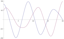
b

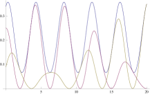
Figure 1: A typical nonlinear Pauli-Schrödinger field in one-dimensional space (here the eigenvalue $\mu=0$). (a) The two spinor components (here, real-valued functions) $\psi_{1}$ (blue) and $\psi_{2}$ (red) are coupled though the nonlinear enthalpy coefficient $H=-2(|\psi_{1}|^{2}+|\psi_{2}|^{2})$, exhibiting chaotic oscillations. (b) The densities $\rho_{1}=|\psi_{1}|^{2}$ (red) and $\rho_{2}=|\psi_{2}|^{2}$ (yellow) oscillates irregularly, while the total density $\rho=\rho_{1}+\rho_{2}$ (blue) remains ordered.

(iii) When the baroclinic terms are finite, there is no one-dimensional (plane wave) solution. In fact, upon substitution of $\psi_{j}=e^{i(k_{y}y+k_{z}z-\omega t)/\hbar}\phi_{j}(x)$ ($j=1,2$) into (8), we obtain an eigenvalue problem

$$\frac{\hbar^{2}}{2m}\frac{d^{2}}{dx^{2}}\phi_{j}=(\lambda+{{H}}-i{{G}}_{j})\phi_{j}\quad(j=1,2),$$ (10)

where $\lambda=(k_{y}^{2}+k_{z}^{2})/2m-\omega$. Half of the (local, i.e., for each $\psi_{j}$) eigenvalues for this operator, $\pm\sqrt{\lambda+{{H}}-i{{G}}_{j}}$, have positive real parts whenever ${{G}}_{j}\neq 0$, and thus, (10) cannot have a bounded solution for any $\lambda$.

The nonexistence of a one-dimensional (plane-wave) solution in a baroclinic system emphasizes the fact that the baroclinic effect is absent in a one-dimensional system. However, we do find interesting solutions in two-dimensional space.

V Quantum spirals

Let us assume a solution of a spiral form:

$$\Psi=\left(\begin{array}[]{c}\psi_{1}\\ \psi_{2}\end{array}\right)=\left(\begin{array}[]{cc}e^{i(n\theta+\beta_{1}(r)-\omega t)}\phi_{1}(r)\\ e^{i(n\theta+\beta_{2}(r)-\omega t)}\phi_{2}(r)\end{array}\right).$$ (11)

The azimuthal mode number $n$ gives the number of arms. The phase factor $\beta_{j}(r)$ determines their shape; for example, when $\beta_{j}(r)$ is a linear function of $r$, we obtain a Archimedean spiral. The factor $\phi_{j}(r)$ yields the radial modulation of amplitudes. We find that the nonlinear terms

$$\rho = \phi_{1}^{*}\phi_{1}+\phi_{2}^{*}\phi_{2},$$ (12)

$$\sigma = \frac{\hbar}{2}\left(\beta_{1}-\beta_{2}+\arg\phi_{1}-\arg\phi_{2}\right)$$ (13)

are functions only of $r$; the azimuthal mode number $n$, therefore, is a good quantum number. Inserting (11) into (8), we obtain ($j=1,2$, $\dot{~{}}$=$d/dr$),

$$\ddot{\phi}_{j}+\left(\frac{1}{r}+i\dot{\beta}_{j}\right)\dot{\phi}_{j}=\left[\left(-\omega+\frac{n^{2}}{r^{2}}+\dot{\beta}_{j}^{2}+{{H}}\right)\right.$$

$$\left.-i\left(\ddot{\beta}_{j}+\frac{\dot{\beta}_{j}}{r}-{{G}}_{j}\right)\right]\phi_{j}.$$ (14)

Bounded solutions are obtained when the non-Hermitian term vanishes; one must, then, solve the system of simultaneous equations

$$\ddot{\phi}_{j}+\left(\frac{1}{r}+i\dot{\beta}_{j}\right)\dot{\phi}_{j} = \left(-\omega+\frac{n^{2}}{r^{2}}+\dot{\beta}_{j}^{2}+{{H}}\right)\phi_{j},$$ (15)

$$\ddot{\beta}_{j}+\frac{\dot{\beta}_{j}}{r}-{{G}}_{j} = 0.$$ (16)

By (16), the baroclinic term $G_{j}$ generates $\beta_{j}(r)$ that determines the shape of spiral. Evidently, in a barotropic field ($G_{j}=0$), spirals do not appear ($\beta_{j}(r)=0$).

To construct explicit examples, let us consider an ideal gas that has an internal energy such that

$${U}=c_{v}(\rho e^{{S}-{\sigma}_{0}})^{1/c_{v}},$$ (17)

where $c_{v}$ (specific heat normalized by Rydberg constant) and ${\sigma}_{0}$ are constants. For simplicity, we assume $S=\sigma$ (thus, $T=\tau$) to evaluate

$${{T}}=(\rho e^{{\sigma}-{\sigma}_{0}})^{1/c_{v}},\quad{{H}}=(c_{v}+1){{T}}.$$ (18)

Substituting (12) and (13), we may write the coefficients $H$ and $G_{j}$ in terms of $\phi_{j}$ and $\beta_{j}$ ($j=1,2$).

As an example ($c_{V}=1$ and $\sigma_{0}=0$) of the numerical solutions of this system, we display in Fig. 2, a typical $n=2$ solution exhibiting twin spirals (opposite sense) of the two components of the spinor $\Psi$. Figure 3 picks up the phase factors $\beta_{j}(r)$ and the amplitude factors $|\phi_{j}(r)|^{2}$ from the spiral spinor fields of Fig. 2.

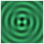
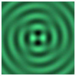
Figure 2: Dual spirals created in a baroclinic Pauli-Schrödinger field; the density plots of $\Re\psi_{1}$ (left) and $\Re\psi_{2}$ (right) show opposite-sense spirals. Here $\omega=4.5$.

a 

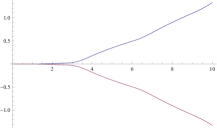
b 

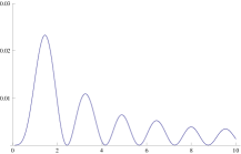
Figure 3: (a) The phase factors $\beta_{1}(r)$ (blue) and $\beta_{2}(r)$ (red) of the quantum spirals shown in Fig. 2. Except in the core region ($r<3$), $\beta_{j}(r)$ is an approximately linear function of $r$, hence the arms are approximately Archimedean. The opposite signs of $\beta_{1}(r)$ and $\beta_{2}(r)$ give opposite-sense spirals. (b) The amplitude factors $|\phi_{1}(r)|^{2}$ ($=|\phi_{2}(r)|^{2}$ by the assumption).

The baroclinic Pauli-Schrödinger equation has axisymmetric ($n=0$) solutions also (see Fig. 4-a).

Figure 4-b shows that when the baroclinic term is zero (then, the generator is Hermitian), no spiral structures, even with a finite $n$, are created. This is because the phase factors $\beta_{j}(r)$ become zero when $G_{j}=0$; see (16).

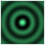
a    b

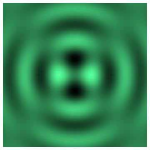
Figure 4: (a) Axisymmetric ($n=0$) solution of the baroclinic equation with $\omega=4.5$; plot of $\Re\psi_{1}$. (b) Barotropic ($G_{j}=0$) Pauli-Schrödinger field ($n=2$) with $\omega=4.5$; plot of $\Re\psi_{1}$. When $G_{j}=0$, the phase factor $\beta_{j}(r)=0$, thus no arms are created.

VI Conclusion

We have shown that the quantum fluid with internal thermal energy is capable of supporting entirely new quantum states like the quantum spirals we have derived in the present simplified model. The harnessing of the profound effect of entropy, in a thermal spin quantum system, has led us to a new mechanism (whose classical counterpart is the famous baroclinic effect generating, for example, hurricanes) that substantially extends the range of vortical states accessible to quantum systems.

We note that although the conventional spin forces (either spin-magnetic field interactions or spin-spin interaction; cf. Appendix A) may amplify or sustain vorticities, they cannot generate it from zero. The baroclinic effect is a creation mechanism that works without a seed. A close analogy is the respective roles of dynamo amplification of magnetic field Moffatt and the Biermann battery mechanism Biermann in a classical plasma; the former needs a seed magnetic field.

We also note that the baroclinic effect we have studied is an isentropic process, and differs from dissipation mechanisms like friction. For example, a finite-temperature Bose gas is modeled by a modified Gross-Pitaevskii equation including an effective friction term, which is coupled with a quantum Boltzmann equation describing a thermal cloud ZNG ; Jackson ; Allen (see also tutorial Proukakis ). The friction term introduces a non-Hermitian Hamiltonian which, in contrast to the presently formulated isentropic model, destroys the conservation of the particle number and the energy of the condensate component.

One expects to find a variety of new/interesting states when this work is extended for more encompassing quantum systems: the thermal Pauli-Schrödinger system and the relativistic thermal Dirac (Feynman-Gellmann) equation coupled to the electromagnetic field. For both of these systems, baroclinic terms can be readily incorporated in known formalisms vortical ; Koide ; mahase2014 . Coriolis force, a close cousin of the magnetic force, could also be included as a gauge field Kambe . When we consider higher-order spinors (for example, spin-1 representation of SU(2) fields may be applied for Bose gas in a trap spin-1 ) the number of Clebsch parameters increases, and the field starts to have a helicity Yoshida_Clebsch .

Appendix A. Correspondence principle

We explain the correspondence principle relating the classical and quantized fields. In terms of the real variables (3), the Hamiltonian (1) reads $\mathscr{H}=\mathscr{H}_{c}+\mathscr{H}_{q}$ with

$$\mathscr{H}_{c} = \int\left[\frac{|\nabla\varphi+\frac{\mu}{\rho}\nabla\sigma|^{2}}{2m}+{U}(\rho,\sigma)\right]\rho\,dx,$$ (19)

$$\mathscr{H}_{q} = \int\frac{\hbar^{2}}{8m}\left(\frac{|\nabla\rho|^{2}}{\rho^{2}}+\sum_{\ell}|\nabla{S}_{\ell}|^{2}\right)\rho\,dx.$$ (20)

Here $\mathscr{H}_{c}$ is a classical Hamiltonian generating fluid dynamics Lin . With the canonical 1-form $\Theta=\int{p}^{0}\rho dx=-\int(\rho\partial_{t}\varphi+\mu\partial_{t}\sigma)\,dx$, the variation of the classical action $\int(\Theta-\mathscr{H}_{c})\,dt$ with respect to the canonical variables $(\rho,\varphi,\mu,\sigma)$ yields Hamilton’s equation:

$$\partial_{t}{\rho} = \partial_{\varphi}\mathscr{H}_{c}=-\nabla\cdot(\bm{v}\rho),$$ (21)

$$\partial_{t}{\varphi} = -\partial_{\rho}\mathscr{H}_{c}=-\bm{v}\cdot\nabla\varphi+m|\bm{v}|^{2}/2-H,$$ (22)

$$\partial_{t}{\mu} = \partial_{\sigma}\mathscr{H}_{c}=-\nabla\cdot(\bm{v}\mu)+\rho T,$$ (23)

$$\partial_{t}{\sigma} = -\partial_{\mu}\mathscr{H}_{c}=-\bm{v}\cdot\nabla\sigma,$$ (24)

where $\bm{v}=\bm{p}/m$ is the fluid velocity, (21) is the mass conservation law, (24) is the entropy conservation law (justifying the parameterization $U(\rho,\sigma)$), and the combination of all equations with the thermodynamic relation $\nabla{{H}}-{{T}}\nabla{\sigma}=\rho^{-1}d{P}$ ($P$ is the pressure) yields the momentum equation

$$\partial_{t}\bm{p}+(\bm{v}\cdot\nabla)\bm{p}=-\rho^{-1}\nabla{P}.$$ (25)

The system (21)-(24) is an infinite-dimensional Hamiltonian system endowed with a canonical Poisson bracket such that

$$\{\rho(\bm{x}),\varphi(\bm{y})\}=\delta(\bm{x}-\bm{y}),~{}\{\mu(\bm{x}),\sigma(\bm{y})\}=\delta(\bm{x}-\bm{y});$$ (26)

all other brackets are zero. By (2) and (3), the Poisson algebra (26) is equivalent to the Lie algebra of the second-quantized Pauli-Schrödinger field acting on the Fock space of either Bosons or Fermions Jackiw :

$$\begin{array}[]{l}{[}\psi_{j}(\bm{x}),\psi_{k}^{*}(\bm{y}){]}_{\pm}=(i\hbar)^{-1}\delta_{jk}\delta(\bm{x}-\bm{y}),\\ {[}\psi_{j}(\bm{x}),\psi_{k}(\bm{y}){]}_{\pm}=0,~{}{[}\psi_{j}^{*}(\bm{x}),\psi_{k}^{*}(\bm{y}){]}_{\pm}=0.\end{array}$$ (27)

Based on this correspondence principle, we can quantize the classical field by adding $\mathscr{H}_{q}$ to $\mathscr{H}_{c}$; the action principle with respect to $\Psi$ yields (8). The same action principle with respect to the real variables (3) yields the fluid representation: on the right-hand side of (25), $\mathcal{H}_{q}$ adds quantum forces tak1 ; tak2

$$\bm{F}_{q}=\nabla\left(\hbar^{2}\frac{\nabla^{2}\sqrt{\rho}}{2m\sqrt{\rho}}\right)-\sum_{\ell}\frac{\hbar^{2}}{4m\rho}\nabla\cdot[\rho\nabla{S}_{\ell}\otimes\nabla{S}_{\ell}],$$ (28)

where ${S}_{\ell}=\rho^{-1}\Psi^{*}\bm{\sigma}_{\ell}\Psi$ ($\bm{\sigma}_{\ell}$ are the Pauli matrices).

References

- (1) London, F. Superfluids, Vol. I: Macroscopic Theory of Superconductivity. (Wiley, 1950).
- (2) London, F. Superfluids, Vol. II: Macroscopic Theory of Superfluid Helium. (Wiley, 1954).
- (3) Landau, L. & Lifshitz, E. Statistical Physics, Chap. VI (Addison-Wesley, 1958).
- (4) Gross, E. P. Structure of a Quantized Vortex in Boson Systems. Nuovo Cimento 20, 454–477 (1961).
- (5) Pitaevskii, L. P. Vortex Lines in an Imperfect Bose Gas, Sov. Phys. JETP 13, 451–454 (1961).
- (6) Hohenberg, P. C. & Martin, P. C. Microscopic theory of superfluid helium, Ann. Phys. 34, 291–359 (1965).
- (7) Fischer, U. R. & Baym, G. Vortex states of rapidly rotating dilute Bose-Einstein condensates, Phys. Rev. Lett. 90, 140402 (2003).
- (8) Fetter, A. L. Rotating trapped Bose-Einstein condensates, Rev. Mod. Phys. 81, 647–691 (2009).
- (9) Mahajan, S. M. Classical Perfect Diamagnetism: Expulsion of Current from the Plasma Interior, Phys. Rev. Lett. 100, 075001 (2008).
- (10) Mahajan, S. M. & Asenjo, F. A. Hot Fluids and Nonlinear Quantum Mechanics, Int J Theor Phys. 54, 1435–1449 (2015).
- (11) Madelung, E. Quantentheorie in hydrodynamischer Form, Z. Phys. 40, 322–326 (1927).
- (12) Bohm, D. A Suggested Interpretation of the Quantum Theory in Terms of “Hidden” Variables. I, Phys. Rev. 85, 166–178 (1952).
- (13) Takabayasi, T. On the Hydrodynamical Representation of Non-Relativistic Spinor Equation, Prog. Theor. Phys. 12, 810–812 (1954).
- (14) Takabayasi, T. The Vector Representation of Spinning Particle in the Quantum Theory I, Prog. Theor. Phys. 14, 283–302 (1955).
- (15) Takabayasi, T. Hydrodynamical description of the Dirac equation, Nuovo Cimento 3, 233–241 (1956).
- (16) Takabayasi, T. Vortex, Spin and Triad for Quantum Mechanics of Spinning Particle I, Prog. Theor. Phys. 70, 1–17 (1983);
- (17) Cufaro Petroni, N., Gueret, Ph. & Vigier, J.-P. A causal stochastic theory of spin-1/2 fields, Nuovo Cimento B 81, 243–259 (1984).
- (18) Fröhlich, H. Microscopic derivation of the equations of hydrodynamics, Physica A 37, 215–226 (1967).
- (19) Haas, F. Quantum plasmas: An Hydrodynamic Approach (Springer, 2011).
- (20) Marklund, M. & Brodin, G. Dynamics of Spin-1/2 Quantum Plasmas, Phys. Rev. Lett. 98, 025001 (2007).
- (21) Brodin, G. & Marklund, M. Spin magnetohydrodynamics, New J. Phys. 9, 277 (2007).
- (22) Mahajan, S. M. & Asenjo, F. A. Vortical Dynamics of Spinning Quantum Plasmas: Helicity Conservation, Phys. Rev. Lett. 107, 195003 (2011).
- (23) Asenjo, F. A., Muñoz, V., Valdivia, J. A. & Mahajan, S. M. A hydrodynamical model for relativistic spin quantum plasmas, Phys. Plasmas 18, 012107 (2011).
- (24) Kaniadakis, G. Statistical origin of quantum mechanics, Physica A 307, 172–184 (2002).
- (25) Pesci, A. I. & Goldstein, R. E. Mapping of the classical kinetic balance equations onto the Schrodinger equation, Nonlinearity 18, 211–226 (2005).
- (26) Pesci, A. I., Goldstein, R. E. & Uys, H. Mapping of the classical kinetic balance equations onto the Pauli equation, Nonlinearity 18, 227–235 (2005).
- (27) Andreev, P. A. & Kuz’menkov, L. S. Problem with the single-particle description and the spectra of intrinsic modes of degenerate boson-fermion systems, Phys. Rev. A 78, 053624 (2008).
- (28) Carbonaro, P. EPL 100, 65001 (2012).
- (29) Koide, T. Spin-electromagnetic hydrodynamics and magnetization induced by spin-magnetic interaction, Phys. Rev. C 87, 034902 (2013).
- (30) Kambe, T. On the rotational state of a Bose-Einstein condensate, Fluid Dyn. Res. 46, 031418 (2014).
- (31) Clebsch, A. Uber die Integration der hydrodynamischen Gleichungen, J. Reine Angew. Math. 56, 1–10 (1859).
- (32) Lin, C. C. Hydrodynamics of Helium II in Proc. Int. Sch. Phys. “Enrico Fermi” XXI 93–146 (Academic Press, 1963).
- (33) Jackiw, R. Lectures on fluid dynamics —a particle theorist’s view of supersymmetic, non-Abelian, noncommutative fluid mechanics and d-branes (Springer, 2002).
- (34) Yoshida, Z. Clebsch parameterization: basic properties and remarks on its applications, J. Math. Phys. 50, 113101 (2009).
- (35) Ho, T.-L. Spinor Bose Condensates in Optical Traps, Phys. Rev. Lett. 81, 742–745 (1998).
- (36) Moffatt, H. K. Magnetic Field Generation in Electrically Conducting Fluids (Cambridge University Press, 1978).
- (37) Biermann, L. Über den Ursprung der Magnetfelder auf Sternen und im interstellaren Raum, Z. Naturforsch. 5a, 65–71 (1950).
- (38) Zaremba, E. , Nikuni, T. & Griffin, A. Dynamics of trapped Bose gases at finite temperatures, J. Low Temp. Phys. 116, 277–345 (1999).
- (39) Jackson, B. , Proukakis, N. P. ,Barenghi, C. F. & Zaremba, E. Finite-temperature vortex dynamics in Bose-Einstein condensates, Phys. Rev. A 79, 053615 (2009).
- (40) Allen, A. J., Zaremba, E. , Barenghi, C. F. &Proukakis, N. P. Observable vortex properties in finite-temperature Bose gases, Phys. Rev. A 87, 013630 (2013).
- (41) Proukakis,N. P. & Jackson, B. Finite-temperature models of Bose-Einstein condensation, J. Phys. B: Atomic, Molecular Optical Phys. 41, 203002 (2008).