Two Stars Two Ways: Confirming a Microlensing Binary Lens Solution with a Spectroscopic Measurement of the Orbit

Abstract

Light curves of microlensing events involving stellar binaries and planetary systems can provide information about the orbital elements of the system due to orbital modulations of the caustic structure. Accurately measuring the orbit in either the stellar or planetary case requires detailed modeling of subtle deviations in the light curve. At the same time, the natural, Cartesian parameterization of a microlensing binary is partially degenerate with the microlens parallax. Hence, it is desirable to perform independent tests of the predictions of microlens orbit models using radial velocity time series of the lens binary system. To this end, we present 3.5 years of RV monitoring of the binary lens system OGLE-2009-BLG-020L, for which Skowron et al. (2011) constrained all internal parameters of the 200–700 day orbit. Our RV measurements reveal an orbit that is consistent with the predictions of the microlens light curve analysis, thereby providing the first confirmation of orbital elements inferred from microlensing events.

1 Introduction

While the general–relativistic microlensing effect has been repeatedly observed, very few direct tests of the microlensing model solutions have been possible. This is because microlensing is inherently a rare transient phenomenon, and the lenses observed are often extremely faint. Because a microlensing event requires that two stars at different distances align with each other along the line-of-sight to better than $\sim 1$ mas, in the densest parts of the sky only about 1 in a million stars is expected to be undergoing a microlensing event at any given time (Paczynski, 1991; Han & Gould, 1995). These events are relatively brief ($\sim 2$ months) and (effectively) unrepeatable. In addition, since the only light required to study the gravitational potential of the foreground lens is provided by the background source, the lens itself can, in principle, be completely non-luminous. Typically, lens stars are M dwarfs that reside more than halfway to the center of the Galaxy at $\gtrsim 4$ kpc, and are thus very faint, making them extremely difficult or impossible to followup after the event is over. This means that while the ensemble of microlensing detections is robust, very few individual lens stars can be studied in detail aside from what can be learned from the lensing event. More importantly, there have been relatively few confirmations of the complex microlensing modeling process even as the number of parameters expands to include more effects.

Most previous tests of microlensing models have focused on confirming that the measured brightness of the lens star is consistent with the predicted lens mass in microlensing. Bennett et al. (2010) made an independent confirmation of a microlensing model based on adaptive optics observations of OGLE-2006-BLG-109. They demonstrated that the observed lens flux is consistent with the predicted lens mass and distance made by measuring the parallax and the finite source effects in the light curve. Likewise Pietrukowicz et al. (2005) discovered a transient in M22 and classified it as likely microlensing event caused by the lens belonging M22 magnifying the background bulge star. They gave mass estimation based on the measured Einstein time-scale, the known distances and globular cluster proper motion ($M=0.14^{+0.10}_{-0.02}M_{\odot}$), which was later confirmed by Pietrukowicz et al. (2012) using VLT/NACO to show that the measured lens flux corresponds to a mass of $M=0.18M_{\odot}$. In addition, Gould (2004) confirmed the microlens parallax measured for MACHO-LMC-5 by showing that the direction of the relative proper motion measured from the separation of the source and lens by Alcock et al. (2001) was consistent with the expectation from the parallax.

In this paper, we present the first direct test of a microlensing detection of orbital motion. While the orbital period at a typical Einstein ring radius of a few AU (where microlensing sensitivity to companions is maximized) is generally much longer than the typical lensing timescale of $t_{\rm E}\sim 20$ days, in some cases it is still possible to observe Keplerian motion of a binary lens system. The theory of orbiting binary lenses was first explored by Dominik (1998). In practice, the detectability of orbital motion depends on having features in the light curve that are well-separated in time ($\sim 20\,$ days) and a relatively short orbital period ($\lesssim$ hundreds of days). The orbital motion leads to changes in the shape of the caustic structure, and hence the magnification pattern due to the changing separation between the components of the lens and can also rotate the caustic on the plane of the sky.

MACHO 97-BLG-41 (Alcock et al., 2000) was the first binary lens to show strong deviations from the assumption of a static binary, but the initial interpretation was that the deviations were due to a third body (a circumbinary planet; Bennett et al., 1999), and it was not until a later analysis of an independent data set that the orbiting binary solution was found (Albrow et al., 2000). This controversy was definitively resolved by Jung et al. (2013), who conducted a combined fit of the data and found that direct comparison of the orbiting binary and circumbinary planet models clearly preferred the binary. Orbital motion is also found in systems in which the companion is a planet, and was in fact observed in the second planetary system discovered by microlensing: OGLE-2005-BLG-071 (Udalski et al., 2005; Dong et al., 2009). Hence, experience has demonstrated that it is important to take these effects into account when fitting microlensing light curves.

At the same time, a test of an orbital motion model would greatly increase our confidence in the derived orbital parameters for both stellar and planetary microlenses. Introducing the orbital motion effect into the microlensing models by definition increases the number of free parameters, raising the concern that any improvement in the fit is due primarily to fitting systematics or correlations in the data. In addition, the orbital motion parameters are known to be correlated with other microlensing parameters and effects such as the orbital parallax effect (the effect of the Earth’s motion on the light curve; see Batista et al., 2011) and xallarap (motion of the source due to a binary). Because of the correlation with parallax, a confirmation of the orbital motion solution will also translate into increased confidence in the measured mass from the parallax effect.

While tests of the orbital motion solutions for stellar lenses with planetary companions will remain difficult even with 30m class telescopes, it is possible that this test could be done for binary star lenses because the orbital motion signal is so much larger (e.g. radial velocities $\mathcal{O}$ km s^-1 for binaries rather than $\mathcal{O}$ m s^-1 for planets).

One system seen to exhibit orbital motion is the binary star lens in OGLE-2009-BLG-020, which was analyzed by Skowron et al. (2011). They found that it was impossible to find a satisfactory fit to the microlensing light curve without allowing for orbital motion of the lens. From this analysis, they were able to place broad constraints on the Keplerian parameters of the orbit (reproduced in the upper, right-hand panels of Figure 4). In brief, the posteriors indicate a $0.84M_{\odot}$ primary with an M-dwarf companion in a 200–700 day orbit with some amount of eccentricity.

What makes this system unusual is that it is exceptionally close for a microlensing lens system, $D_{\rm L}\sim 1\,$ kpc, such that the lens is clearly visible in the blended light. In fact, with an $I$ magnitude of 15.6, the lens is brighter than the unmagnified source. Because the system is so bright and the expected radial velocity (RV) signal from the lens is so large ($\sim 10$ km s^-1), it is possible to confirm the orbital motion of the lens system measured from the microlensing light curve with followup observations.

In this paper, we present radial velocity followup observations of the lens system and confirm a microlensing orbit solution for the first time. We begin by comparing and contrasting the direct observables of binary stars as seen with radial velocity and microlensing (Section 2). The microlensing and RV observations of OGLE-2009-BLG-020  are presented in Section 3. A detailed discussion of the RV data is given in Section 4 including a novel method to use the source star as a wavelength reference (Section 4.2) and the final RV solution to the orbit (Section 4.4). In Section 5, we show that this RV solution is consistent with the constraints on the orbit from Skowron et al. (2011), and in Section 6 we perform a joint fit to both the RV and microlensing data to find the final parameters of the binary system. Our conclusions are given in Section 7.

2 Orbit Kinematics: RV vs. Microlensing Observables

Table 1: Standard, Keplerian Parameterization of a Binary

Variable	Units	Meaning
Binary Orbit Parameters:
$t_{\rm peri}$	days	Time of periastron
$a$	AU	Semi-major axis
$e$	$\cdots$	Eccentricity
$\Omega_{\rm node}$	deg	Longitude of ascending node
$i$	deg	Inclination
$\omega_{\rm peri}$	deg	Argument of periastron
$m_{1}$	$M_{\odot}$	Mass of primary
$m_{2}$	$M_{\odot}$	Mass of secondary
Phase-Space Parameters:
$D_{L}$	kpc	Distance to system
$\theta$	deg	Coordinates of the system (RA/DEC)
$\mu$	mas yr-1	Proper motion of the system
$v_{z}$	km s-1	Radial velocity of the system

Table 2: RV Parameterization of a Binary

Variable	Units	Meaning
RV Orbit Invariants:
$t_{\rm peri}$	days	Time of periastron
$P$	days	Period
$e$	$\cdots$	Eccentricity
$\omega_{\rm peri}$	deg	Argument of periastron
${\cal M}=(m_{2}\sin i)^{3}/(m_{1}+m_{2})^{2}$		Mass function
($m_{1}$	$M_{\odot}$	Spectroscopic mass of primary)
Other known/measured parameters:
$\theta$	deg	Coordinates of the system (RA/DEC)
$v_{z}$	km s-1	Radial velocity of the system

RV Observables:
   $t_{\rm peri}$ days Time of periastron
   $P$ days Period
   $e$  $\cdots$  Eccentricity
   $\omega_{\rm peri}$ deg Argument of periastron
   $K$ km s^-1 RV semi-amplitude

Table 3: Microlensing Parameters

Variable	Units	Meaning
13 Parameters of a Microlensing Model:
$u_{0}$	$\theta_{\rm E}$	Closest approach between the source and lens
$t_{0}$	days	Time when $u(t)=u_{0}$
$t_{\rm E}$	days	Einstein crossing time
$\rho$	$\theta_{\rm E}$	Normalized source size
${\mbox{\boldmath$\pi$}}_{\rm E}$	$\cdots$	Microlens parallax vector
$s$	$\theta_{\rm E}$	Projected separation of the lens components
$q$	$\cdots$	Mass ratio between the lens components
$\alpha$	rad	Angle between the binary axis and the source trajectory
$\gamma$	$\cdots$	Normalized, projected relative velocity of the binary
$s_{z}$	$\theta_{\rm E}$	Relative position of the lens companion along the line of sight
$\gamma_{z}$	$\theta_{\rm E}$	Relative velocity of the binary along the line of sight
Additional Known Parameters:
$\theta$	deg	Angular coordinates of the microlensing event (RA/DEC)
$\theta_{\star}$	mas	Angular size of the source
$\pi_{\rm S}$	mas	Source parallax

Table 4: Parameters Derived from Microlensing Parameters

Variable	Definition	Units	Meaning
Intermediate Parameters:
$\theta_{\rm E}$	$\theta_{\star}/\rho$	mas	Angular size of the Einstein ring
$\mu_{\rm geo}$	$\theta_{\rm E}/t_{\rm E}$	mas yr-1	Geocentric relative proper motion between the source
			and lens (magnitude)
$\hat{{\mbox{\boldmath$\mu$}}}_{\rm geo}$	$\hat{{\mbox{\boldmath$\pi$}}}_{\rm E}$	$\cdots$	Direction of geocentric relative proper motion
${\bf s}$	($s\cos\alpha,s\sin\alpha$)	$\theta_{\rm E}$	Projected binary separation vector
$\Delta{\mbox{\boldmath$\theta$}}$	${\bf s}\theta_{\rm E}$	mas	Angular binary separation
$M_{\rm tot}$	$\theta_{\rm E}/(\kappa\pi_{\rm E})$	$M_{\odot}$	Total mass of binary
Binary Parameters:
$m_{1}$	$M_{\rm tot}/(1+q^{-1})$	$M_{\odot}$	Mass of primary primary
$m_{2}$	$m_{1}/q$	$M_{\odot}$	Mass of secondary
$D_{L}$	AU$/(\theta_{\rm E}\pi_{\rm E}+\pi_{\rm S})$	kpc	Distance to the binary system
${\bf r}_{\perp}$	$D_{L}{\mbox{\boldmath$\theta$}}$	AU	Physical position of the binary system
${\bf v}_{\perp}$	$D_{L}{\mbox{\boldmath$\mu$}}_{\rm geo}$	km s-1	Projected velocity of the binary system
$\Delta{\bf r}_{\perp}$	$D_{L}\Delta{\mbox{\boldmath$\theta$}}$	AU	Physical projected separation of the secondary
$\Delta r_{z}$	$D_{L}s_{z}\theta_{\rm E}$	AU	Relative position of the secondary along the line of sight
$\Delta{\bf v}_{\perp}$	$D_{L}s\theta_{\rm E}\hfil\lx@intercol\mbox{\boldmath$\gamma$}$	km s-1	Relative, projected velocity of the secondary
$\Delta v_{z}$	$D_{L}\gamma_{z}\theta_{\rm E}$	km s-1	Relative velocity of the secondary along the line of sight
($v_{z}$	$\cdots$	$\cdots$	Unknown systemic radial velocity)

Fourteen parameters are required to completely characterize the kinematics of a binary star orbit. These could be the six phase-space coordinates of each body at a given time plus its mass, or any non-degenerate set of combinations of these quantities, for example those given in Table 1. Single-line spectroscopic (RV) observations yield measurements nine of these 14 parameters, while microlensing observations can potentially yield 13. However, the natural parameterizations of these two characterizations are very different. Hence, before comparing microlensing predictions with RV measurements, it is essential to understand each parameterization.

2.1 Radial Velocity Parameters

RV observations are normally thought of as yielding five (out of eight) parameters that characterize the internal motion of the binary, plus a spectroscopic estimate of the mass of the primary. These are the period $P$, the eccentricity $e$, the argument of periastron $\omega$, the time of periastron $t_{\rm peri}$, and the mass function ${\cal M}=(m_{2}\sin i)^{3}/(m_{1}+m_{2})^{2}$. These are the same as the RV observables except that the invariant ${\cal M}$ is replaced by the observable $K$, the RV semi-amplitude. Of the remaining parameters that are not measured, the longitude of ascending node ($\Omega$), is rarely of physical interest and is therefore usually ignored. Thus, there are only two parameters of interest that are not measured, the inclination $i$ and the mass ratio $q=m_{2}/m_{1}$. Note that for double-lined binaries, $q$ is measured, while for extreme mass ratios (e.g., planets), ${\cal M}\simeq(q\sin i)^{3}m_{1}$.

For RV, three center-of-mass parameters are also known, namely the measured system radial velocity, $v_{z}$, and the two-dimensional position on the sky ($\theta$, i.e. the coordinates of the system in right ascension and declination). The last two are so intrinsic to the process of measurement that they are not normally even considered as “measurements”.

Table 2 summarizes the binary parameters known from RV observations.

2.2 Microlensing Parameters

Since microlensing can in principle measure 13 parameters, the simplest way to characterize these is to specify the parameter that cannot be measured: the system radial velocity. In addition, microlensing cannot distinguish between $(\Omega,\omega_{\rm peri})$ and $(180\,{\rm deg}-\Omega,\omega_{\rm peri}-180\,{\rm deg}$ (Skowron et al., 2011). That is, the parameters that can be derived from microlensing are identical to those from astrometric measurements for similar reasons: namely that microlensing effects derive from the time evolution of the projected positions of the two components on the plane of the sky.

However, from the standpoint of understanding the information content of microlens binary solutions, the above description is a bit too simple. First, several of the microlensing parameters are quite unfamiliar combinations of phase-space and masses. More important, the precision with which these parameters can be measured is highly variable, with some parameters measured to fractions of a percent and others usually measured only to within a factor of a few (with notable exceptions in Shin et al., 2011, 2012). Properly understanding how RV and microlensing can be compared requires taking these differences into account.

First we consider the parameters that are required to characterize a caustic-crossing binary microlensing event, which can then be transformed into 13 physical parameters of the binary. Seven parameters describe the basic microlensing event. Three of these describe the underlying point-lens event, i.e., the time of maximum $t_{0}$, the impact parameter $u_{0}$ (in units of the angular Einstein radius $\theta_{\rm E}$), and the Einstein timescale $t_{\rm E}$. There are three basic binary lens parameters, the mass ratio $q$ and the vector projected separation ${\bf s}$ of the companion (in units of $\theta_{\rm E}$) relative to the direction of lens-source relative proper motion in the geocentric frame ${\mbox{\boldmath$\mu$}}_{\rm geo}$. This vector is frequently expressed as ${\bf s}=(s\cos\alpha,s\sin\alpha)$, where $\alpha$ is the angle between the binary axis and the source trajectory. Finally, there is the normalized source size $\rho=\theta_{*}/\theta_{\rm E}$, which is required to described the extended duration of the caustic crossing due to the finite angular size of the source $\theta_{*}$. Of these 7 parameters $(t_{0},u_{0},t_{\rm E},q.\,{\bf s},\rho)$ all but two ($t_{0},u_{0}$) enter the 13-parameter binary characterization.

The accelerated motion of Earth can induce sufficient distortions in the lightcurve to measure the “microlens parallax” (Gould, 1992).

$${\mbox{\boldmath$\pi$}}_{\rm E}\equiv{\pi_{\rm rel}\over\theta_{\rm E}}{{\mbox{\boldmath$\mu$}}_{\rm geo}\over\mu_{\rm geo}},$$ (1)

where $\pi_{\rm rel}={\rm AU}(D_{L}^{-1}-D_{S}^{-1})$ is the lens-source relative parallax (see Gould & Horne (2013) for a didactic explanation).

Because microlensing observations are short compared to an orbital period, the orbital parameters are naturally formulated in terms of Cartesian phase-space coordinates, rather than Kepler invariants (as for RV). In addition, because the microlensing event is entirely governed by the projected motion of the binary, the most robustly measured parameter of the motion is the projected, relative velocity of the binary, $\Delta{\bf v}_{\perp}$. This is parameterized as instantaneous rates of change of $s$ and $\alpha$ respectively, which yield $\mbox{\boldmath$\gamma$}=(\gamma_{\parallel},\gamma_{\perp})\equiv(ds/dt/s,d\alpha/dt)$.

The remaining two parameters $(\Delta r_{z},\Delta v_{z})$ must be inferred from the impact of acceleration on the second derivatives of $s$ and $\alpha$. There is no particular reason to express the final two parameters as $(\Delta r_{z},\Delta v_{z})$; they might, for example, be just as well written as the instantaneous angular acceleration. Regardless, because microlensing events last only a small fraction of an orbital period, clearly any such measurements must be substantially less precise than the other parameters. Nevertheless, all 13 parameters have been well measured in at least 4 cases (OGLE-2005-BLG-018, OGLE-2009-BLG-020,MOA-2011-BLG-090, OGLE-2011-BLG-0417; Shin et al., 2011; Skowron et al., 2011; Shin et al., 2012; Gould et al., 2013).

We now explain how these light curve parameters can be transformed into physical properties. With the exception of $v_{z}$ and the sign of $\Delta r_{z}$, all 13 binary parameters can be recovered with various combinations of the known parameters.

As in RV, $\theta$ is automatically measured. In addition, the measurement of $\rho$ enables a determination of $\theta_{\rm E}$. This is because the fit to the light curve yields the source flux and so, if there are measurements in two bands, the position of the source on an instrumental color-magnitude diagram and hence the dereddened flux $F$ and surface brightness $S$, and so finally $\theta_{*}=\sqrt{F/\pi S}$ (Yoo et al., 2004). Then $\theta_{\rm E}=\theta_{*}/\rho$, which allows the transformation of three others into more familiar form

$$\mu_{\rm geo}={\theta_{\rm E}\over t_{\rm E}};\qquad\Delta{\mbox{\boldmath$\theta$}}={\bf s}\theta_{\rm E},$$ (2)

where $\Delta{\mbox{\boldmath$\theta$}}$ is the instantaneous angular separation between the two components.

The combination of ${\mbox{\boldmath$\pi$}}_{\rm E}$ and $\theta_{\rm E}$ then add three more binary parameters. First, of course, ${\mbox{\boldmath$\pi$}}_{\rm E}$ immediately yields the direction of ${\mbox{\boldmath$\mu$}}_{\rm geo}$. Then, because

$$\theta_{\rm E}^{2}=\kappa M\pi_{\rm rel},\qquad\kappa\equiv{4G\over{\rm AU}\,c^{2}}\simeq 8.1\,\frac{\rm mas}{M_{\odot}},$$ (3)

(Einstein, 1936) and because $\pi_{s}$ is usually known quite well, we obtain the mass and distance of the system

$$M={\theta_{\rm E}\over\kappa\pi_{\rm E}};\qquad D_{l}={{\rm AU}\over\theta_{\rm E}\pi_{\rm E}+\pi_{s}}.$$ (4)

The measurement of $D_{L}$ enables us to transform angular measurements into physical measurements, i.e., $\Delta{\bf r}_{\perp}=D_{L}\Delta{\mbox{\boldmath$\theta$}}$, ${\bf v}_{\perp}=D_{L}{\mbox{\boldmath$\mu$}}_{\rm geo}$, and ${\bf r}_{\perp}=D_{L}{\mbox{\boldmath$\theta$}}$. Hence, we now have 9 parameters, $(m_{1},m_{2},{\bf r},{\bf v}_{\perp},\Delta{\bf r}_{\perp})$ where ${\bf r}$ is the 3-space position of the lens system at $t_{0}$. Finally, via the other measurement parameters, these yield $\Delta{\bf v}_{\perp}=D_{L}s\theta_{\rm E}\mbox{\boldmath$\gamma$}$ and so 13 parameters $(m_{1}$, $m_{2}$, $D_{L}$, ${\bf r}_{\perp}$, ${\bf v}_{\perp}$, $\Delta{\bf r}_{\perp}$, $\Delta{\bf v}_{\perp}$, $\pm\Delta r_{z}$, $\Delta v_{z})$.

Table 3 summarizes the microlensing parameters, and Table 4 gives an overview of how those parameters translate into the parameters of a binary. Appendix B of Skowron et al. (2011) provides additional details on the transformation between microlensing parameters and the parameters of a Keplerian orbit.

2.3 RV vs. Microlensing: Points of Comparison

To understand the conditions under which binary microlensing observations can be tested by RV, we now focus on 10 parameters, namely the six phase-space coordinates of internal motion ($\Delta{\bf r},\Delta{\bf v}$), the two masses (($m_{1},m_{2}$), or equivalently $(M,q)$), the system distance ($D_{L}$ or $r_{z}$) and the direction of transverse motion (${\mbox{\boldmath$\mu$}}/\mu$). We therefore ignore the system radial velocity ($v_{z}$), which can be measured very well by RV but not at all by microlensing, the magnitude of the proper motion ($\mu$), for which the reverse holds true, as well as the system angular coordinates $({\mbox{\boldmath$\theta$}})$, which were included only for completeness.

RV observations measure 5 combinations of these quantities, namely four internal phase-space coordinates and the mass function, which is a combination of $m_{1}$, $m_{2}$, and $i$. Here, we ignore for the moment the fact that spectroscopic measurements also return an estimate of the primary mass $m_{1}$.

We begin the analysis of microlensing by examining the “typical good case”, in which ($q$, ${\bf s}$, $\theta_{\rm E}$, ${\mbox{\boldmath$\pi$}}_{\rm E}$, $\gamma$) are measured, while $(\Delta r_{z},\Delta v_{z})$ are not measured. These eight measured quantities are all combinations of the ten parameters under consideration. That is $(q,{\mbox{\boldmath$\pi$}}_{\rm E},\theta_{\rm E})\leftrightarrow(m_{1},m_{2},D_{L},{\mbox{\boldmath$\mu$}}/\mu)$, and $(\Delta{\bf r}_{\perp},\Delta{\bf v}_{\perp})\leftrightarrow D_{L}\theta_{\rm E}({\bf s},s\mbox{\boldmath$\gamma$})$. Hence, with a total of 8 microlensing plus 5 RV $=13$ constraints on a total of 10 parameters, there are nominally three independent points of comparison.

However, in the case of OGLE-2009-BLG-020, the situation is not quite so favorable. There is a well-known degeneracy between $\gamma_{\perp}$ and $\pi_{{\rm E},\perp}$, the component of ${\mbox{\boldmath$\pi$}}_{\rm E}$ parallel to the projection of Earth’s acceleration on the plane of the sky (Batista et al., 2011), and this degeneracy is present in the solution of OGLE-2009-BLG-020 as well (Skowron et al., 2011). Hence, in fact, there are only two independent points of comparison in the present case.

In addition, if we consider that RV is returning six of the 10 parameters (i.e., including the spectroscopic determination of the mass) then the parameter counting yields $6+8-1-10=3$ independent points of comparison. In the present work, we will not consider the mass test due to the low signal-to-noise of the spectra. Nevertheless, it is clear that with by combining microlensing and RV observations, the problem is over-constrained, allowing a direct test of the microlensing orbit prediction.

3 Observations

3.1 Microlensing Data

The microlensing data on OGLE-2009-BLG-020  are described in detail in Section 2 of Skowron et al. (2011) and shown in their Figure 1. In brief, the event was monitored by the Optical Gravitational Lensing Experiment (OGLE) and Microlensing Observations in Astrophysics (MOA) survey groups. In addition, it was observed by eight followup telescopes: Bronberg Observatory 36cm, Campo Catino Austral Observatory 40cm, CTIO/SMARTS 1.3m, Farm Cove Observatory 36cm, Faulkes Telescope North 2.0m, Faulkes Telescope South 2.0m, Kumeu Observatory 36cm, and University of Tasmania 1.0m. As described in Section 2.2 of Skowron et al. (2011), the data have had outliers removed, been binned, and had the error bars rescaled so that $\chi^{2}_{d}/{\rm dof}\sim 1$ for each data set.

3.2 Keck/HIRES

Between Mar 2011 and Oct 2011 OGLE-2009-BLG-020 was observed six times by the HIgh-Resolution Echelle Spectrometer (HIRES; Vogt et al., 1994) on the Keck I telescope with an exposure time of 700s. One additional observation was taken in Aug 2013 with an exposure time of 900s. All the spectra were taken without the iodine cell and $R\approx 55,000$. A summary of observations is given in Table 5.

These data were reduced using the standard California Planet Search (CPS) pipeline (Howard et al., 2010).

3.3 Magellan/MIKE

Seven of the observations were taken with the red camera of the Magellan Inamori Kyocera Echelle spectrometer (MIKE; Bernstein et al., 2003) on the 6.5m Magellan/Clay telescope. The observations are summarized in Table 5. Most of the observations were taken with the $0.7^{\prime\prime}$ slit with a 900 second exposure time. The exceptions were observations on 24 May 2014 and 5 September 2014, which were taken in poor seeing conditions ($2^{\prime\prime}$ and $>3^{\prime\prime}$, respectively).

These spectra were reduced using the CarPy MIKE pipeline (Kelson et al., 2000; Kelson, 2003). Each spectrum was reduced individually with the exception of the observations of 5 September 2014. In that case, we use the MIKE pipeline to stack the four spectra to increase the signal-to-noise ratio (S/N). The wavelength calibration was done relative to ThAr lamp observations taken before and/or after the science exposures. We removed the blaze by fitting the continuum of each order with a (Gaussian)+(Constant)+(Slope), i.e.,

$$f(x)=p_{1}\exp\left(\frac{-(x-p_{2})^{2}}{2p_{3}}\right)+p_{4}+p_{5}x.$$ (5)

This results in a flatter continuum than the standard CarPy reduction. However, the differences in the resultant RVs are minimal. We find that our method results in slightly smaller RV uncertainties $\sim 10$–20%, but the difference in the measured RVs between the two methods is ($\lesssim 0.1$ km s^-1) is an order of magnitude smaller than the values of the uncertainties ($\sim 0.5$–$1$ km s^-1).

4 Radial Velocities

Table 5: RVs of OGLE-2009-BLG-020

BJD′	RV	$\sigma_{\rm RV}$	Observatory	Instr	Date	Slit	Exposure	Resolution	S/N @
	(km s-1)						Time (s)		6000Å
5635.1293	-36.23	0.88	Keck I	HIRES	14 Mar 2011	0.861”	700	55,000	10
5668.0545	-40.37	0.90	Keck I	HIRES	16 Apr 2011	0.861”	700	55,000	12
5708.0989	-42.77	1.35	Keck I	HIRES	26 May 2011	0.861”	700	55,000	8
5723.9147	-44.12	0.93	Keck I	HIRES	11 Jun 2011	0.861”	700	55,000	10
5797.7612	-43.82	0.74	Keck I	HIRES	24 Aug 2011	0.861”	700	55,000	13
5843.7469	-37.06	0.27	Keck I	HIRES	9 Oct 2011	0.861”	700	55,000	8
6530.7713	-42.96	1.63	Keck I	HIRES	26 Aug 2011	0.861”	900	55,000	12
6586.4889	-44.38	0.85	Magellan/Clay	MIKE	20 Oct 2013	0.7”	900	31,000	10
6586.5058	-44.30	0.52	Magellan/Clay	MIKE	20 Oct 2013	0.7”	900	31,000	12
6721.8966	-33.81	0.99	Magellan/Clay	MIKE	4 Mar 2014	0.7”	900	31,000	15
6722.8966	-33.23	0.56	Magellan/Clay	MIKE	5 Mar 2014	0.7”	900	31,000	17
6801.8221	-42.13	0.98	Magellan/Clay	MIKE	24 May 2014	1.0”	900	22,000	7
6906.5487	-42.83	0.67	Magellan/Clay	MIKE	5 Sep 2014	0.7”	6900	31,000	7
6908.6027	-43.25	0.44	Magellan/Clay	MIKE	7 Sep 2014	0.7”	1800	31,000	25

Figure 1: Typical maximum likelihood functions for the spectrum of OGLE-2009-BLG-020 from Keck/HIRES (left) and Magellan/MIKE (right). The taller peak corresponds to the lens primary and the fainter peak to the source star. The velocity scale is arbitrary.

4.1 RV template

To determine the radial velocities of the lens primary, we cross-correlate the spectra of OGLE-2009-BLG-020  with a template from the CPS database. Because the default CPS pipeline only produces a flattened and stitched spectrum of HIP63762  covering the wavelength range $5010\AA$–$6309\AA$, we use only the orders of the HIRES spectrum of OGLE-2009-BLG-020 that overlap with that region (i.e. orders 0–14). We combine the individual CCFs for each order to create a maximum likelihood function (ML) following the prescription in Zucker (2003). This produces a double-peaked ML in which the taller peak corresponds to the (brighter) lens and the smaller peak to the source (see Figure 1).

We selected the template by cross-correlating the highest S/N Keck spectrum (from BJD${}^{\prime}=5797.7612$) with spectra of all stars in the CPS database and measuring the heights of both the source and lens peaks. We find that the lens is broadly consistent with being an early K-dwarf and select our template from amongst the 10 best matches with $5.5\leq M_{V}\leq 8.5$ and $0.85\leq(B-V)\leq 1.35$ (cuts that encompass most stars with likelihood peaks within 95% of the maximum value). Note that our template choice, HIP63762, is also broadly consistent with the source spectrum, obviating the need for a two template fit. Because the source is a clump giant and the CPS sample specifically selects against giants, it is unsurprising that the best available template for the source would be a dwarf of similar color.

4.2 Keck Velocities

To determine the radial velocity of the lens and source for each epoch, we calculate the ML of OGLE-2009-BLG-020  as compared to HIP63762  in the manner described above. We then fit the two tallest peaks of the ML with 3, 4, and 5 parameter Gaussians (see Equation 5), and take the result with the best $\chi^{2}$. The measured lag of each peak is then the value of $p_{2}$ for the best fit.

Because the source star has a constant velocity (confirmed by applying a barycentric correction to the measured lag), we can use it as a wavelength reference in a manner analogous to an iodine cell. Both the source and the lens spectra encounter the same systematic effects as their light passes through the telescope and instrument optics. Hence, we take the measured RV of the lens to be

$${\rm RV}_{\rm lens}={\rm lag}_{\rm source}-{\rm lag}_{\rm lens},$$ (6)

where ${\rm lag_{source}}$ and ${\rm lag_{lens}}$ are the lags of the source and lens, respectively, measured relative to HIP63762. This automatically takes into account (and removes) the barycentric velocity and other systematics induced by the instrument. The uncertainty of the RV is taken to be the standard deviation of the RVs measured for each individual order using the same method (i.e., ${\rm RV}_{{\rm lens},i}={\rm lag}_{{\rm source},i}-{\rm lag}_{{\rm lens},i}$). The uncertainties in the RVs are dominated by uncertainties in the measurement of the source peak. These uncertainties are larger than they would be if we simply made a barycentric correction to the measured velocity of the lens peak. However, the RVs using our method are sufficiently precise for characterizing the system and likely to be more accurate because our method automatically accounts for systematic effects. The final velocities are given in Table 5 where BJD${}^{\prime}={\rm BJD_{\rm TBD}}-2450000$.

4.3 Magellan Velocities

For the Magellan/MIKE spectra, we used only the orders from the red camera that overlapped with the iodine region, i.e. orders 57-68 (12 total). We also cross-correlate those orders against the flattened Keck/HIRES spectrum of HIP63762. We create the ML and extract the lag of tallest peak in the same way as for the Keck data. However, as can be seen from Figure 1, the ML (and CCFs) for the Magellan/MIKE spectra are lower resolution and lower S/N than the Keck/HIRES spectra, and so we are not able to reliably extract the lag of the source using this method. Instead, we calculate the barycentric correction explicitly for each observation using BARYCORR (Wright & Eastman, 2014) and apply it to the measured lens RV. This leaves a velocity offset between the Magellan RVs and the Keck RVs equivalent to the difference in radial velocity between the source star and the template. We can place the Magellan lags on the same velocity scale as the Keck RVs by calculating this difference, i.e. the weighted mean lag of the source star in the Keck data ($<{\rm lag}_{\rm source,K}>$) after the barycentric velocity has been removed. Hence, the Magellan velocities on the Keck system are given by

$${\rm RV}_{\rm lens}=<{\rm lag}_{\rm source,Keck}>-({\rm lag}_{\rm lens,Mag}-{\rm BC}).$$ (7)

To compute the uncertainty in the radial velocities from the Magellan data, we first compute the uncertainty in ${\rm RV}_{\rm lens}$ by computing the standard deviation of ${\rm RV}_{\rm lens}$ measured for each order individually, as we did for the Keck data. Then, we add this in quadrature to the standard deviation of $<{\rm lag}_{\rm source,Keck}>$ as measured from the Keck MLs ($\sigma_{\rm<lag_{source}>}=0.29\,{\rm km\,s}^{-1}$). Final values for the radial velocities are given in Table 5.

4.4 RV Orbit

Table 6: RV Parameters: Median values and 68% confidence interval for OGLE-2009-BLG-020

Parameter	Units	RV-only
RV Orbit Parameters:
$t_{\rm peri}$	Time of periastron (      $\rm{BJD_{TDB}}$)		$6142.7_{-1.9}^{+2.5}$
$P$	Period (days)	$276.37_{-0.91}^{+0.96}$
$e$	Eccentricity	$0.335_{-0.056}^{+0.074}$
$\omega_{\rm peri}$	Argument of periastron (degrees)	$156.8\pm 3.4$
$\cal M$	Mass Function	$6.20_{-0.95}^{+2.08}\times 10^{-3}$
Other Parameters:
$a$	Semi-major axis (AU)	$0.8467\pm 0.0076$
$K$	RV semi-amplitude (km/s)	$6.370_{-0.450}^{+0.880}$

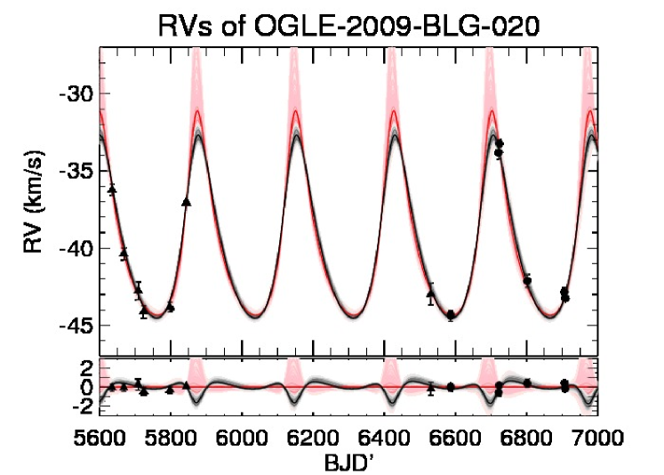
Figure 2: Measured radial velocities of OGLE-2009-BLG-020L. The red line shows the best-fit orbit to the RV data alone, and the black line shows the best-fit orbit from the joint MCMC including both the RV and microlensing data. The gray (and pink) liness show joint (and RV-only) fits that are 1, 2, and 3-$\sigma$ from the best fit (reflected by the shading).

We use EXOFAST (Eastman et al., 2013) to find the best-fit orbit to the radial velocity data of OGLE-2009-BLG-020. This package finds preliminary solutions using a Lomb-Scargle periodogram, refines them using an Amoeba minimization, and determines the uncertainties using a Markov Chain Monte Carlo. We began by finding a preliminary solution for the period using a Lomb-Scargle periodogram and then seed EXOFAST with this value as a prior. We allow for free eccentricity but do not allow for a slope, such as might be caused by a third body in the system. EXOFAST uses BJD as the time standard.

These fits clearly indicate that our uncertainties for the radial velocities are over-estimated, and rescales them by 0.4255. This fit shows that the lens has a period of $\sim 276$ days and an eccentricity of 0.341. The red line in Figure 2 shows the best-fit RV curve to the data. The full RV solution (parameters and their uncertainties) is given in Table 6. The posteriors are shown in the lower-left panels of Figure 3. Note that EXOFAST provides the argument of periastron of the primary $\omega_{\star}$. We report the argument of periastron of the secondary $\omega_{\rm peri}\equiv\omega_{\star}-180\,{\rm deg}$.

5 Comparison of Independent Fits

Table 7: Joint Fit: Orbit Parameters

Parameter	Units	Value	Uncertainty
Eccentricity	…	$0.265$	$\pm 0.025$
$a$	AU	$0.865$	$\pm 0.024$
$t_{\rm peri}$	days	$4758.692$	$\pm 2.685$
$\Omega_{\rm node}$	deg	$-7.767$	$\pm 1.260$
inclination	deg	$129.424$	$\pm 1.238$
$\omega_{\rm peri}$	deg	$151.600$	$\pm 3.325$
$M_{\rm tot}$	$M_{\odot}$	$1.132$	$\pm 0.097$
$D_{\rm L}$	kpc	$0.747$	$\pm 0.020$
$q$	…	$0.275$	$\pm 0.003$
Derived:
Period	days	$276.555$	$\pm 0.300$
$m_{1}$	$M_{\odot}$	$0.244$	$\pm 0.021$
$m_{2}$	$M_{\odot}$	$0.888$	$\pm 0.076$

Figure 3 compares the RV constraints on the orbit of OGLE-2009-BLG-020L (Section 4.4) derived from EXOFAST to the independent constraints on the orbit from the microlensing light curve (Skowron et al., 2011). The microlensing constraints include the weighting for the Jacobian, the Galactic model, and lens flux as described in Sections 3.4 and 4.2.1 of Skowron et al. (2011). For the purposes of this comparison, we extrapolate $t_{\rm peri}$ for the RV fit backwards to the time of the microlensing observations. In addition, note that microlensing uses $HJD$ as the time standard rather than $BJD$, but this difference is many orders of magnitude smaller than the uncertainties in the measured parameters.

The constraints on the RV parameters from the microlensing light curve are derived from the MCMC fits to the microlensing data in Skowron et al. (2011). Because of the $\pm$ degeneracy in $(s_{z},\gamma_{z})$ measured from microlensing, there is a perfect degeneracy between $\omega_{\rm peri}$ and $\omega_{\rm peri}-180\,{\rm deg}$. Since both are equally valid, we plot both solutions in Figure 3 leading to periodic behavior in $\omega_{\rm peri}$.

Figure 3œ clearly shows that the constraints on the orbit of OGLE-2009-BLG-020L from the radial velocity data are consistent with the observed properties of the orbit measured from the microlensing light curve. This is the first confirmation of orbital motion of a 2-body system measured from a microlensing light curve.

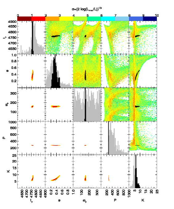
Figure 3: A comparison of the orbit constraints for OGLE-2009-BLG-020L from independent fits to the microlensing light curve (upper right; Skowron et al., 2011) and the radial velocities (lower left; EXOFAST, Section 4.4). In the upper right panels, the black contours show the RV constraints overplotted on the microlensing constraints. The center panels on the diagonal compare the posteriors (gray: microlensing, black: radial velocity). For the microlensing constraints, the colors represent the weights of each link as described in Skowron et al. (Section 3.4 of 2011). For the RVs, the colors reflect the likelihood as determined from the $\chi^{2}$ of each fit.

6 Joint Fit

We also perform a joint MCMC fit to the RV and microlensing data to determine the best constraints on the physical properties of the OGLE-2009-BLG-020L system. The joint MCMC is performed in the same parameter space as in Skowron et al. (2011), i.e. using $t_{0}$, $u_{0}w$, $t_{\rm eff}$, $t_{\star}$, $\pi_{\rm E,E}$, $\pi_{\rm E,N}$, $\alpha$, $\gamma_{\parallel}$, $\gamma_{\perp}$, $s_{z}$, $\log q$, $\log w$, and $\gamma_{z}$ as the MCMC parameters. These parameters are similar to those in Table 3, with a few substitutions. In place of $t_{\rm E}$ and $\rho$ we have $t_{\rm eff}\equiv u_{0}t_{\rm E}$ and $t_{\star}\equiv\rho t_{\rm E}$. In addition, we use the caustic width $w$ instead of $s$ and $u_{0}w$ instead of $u_{0}$ and step in the $\log$ of $q$ and $w$. As described in Skowron et al. (2011), this parameterization results in faster convergence of the MCMC.

In addition, we include the angular size of the source, $\theta_{\star}$, as a chain parameter. Although this is an observable quantity ($\theta_{\star,0}=4.45\,\mu$as, see Section 4.1.1 of Skowron et al. 2011), it has some uncertainty (7%) for which we want to allow in the Markov chain. To do this, we allow this parameter to float, but we apply a $\chi^{2}$ penalty for values that deviate from the observed value, i.e.

$$\chi^{2}_{\rm penalty}=\left(\frac{\theta_{\star}-\theta_{\star,0}}{\theta_{\star,0}}\frac{1}{0.07}\right)^{2}.$$ (8)

Finally, we change the sign of the RV data to account for the sign difference in the RV and microlensing coordinate systems (Skowron et al., 2011).

For each link, the MCMC parameters are converted to binary orbit parameters, which are used to generate an RV curve. The degeneracy in $\pm(s_{z},\gamma_{z})$ leads to a degeneracy in the sign of the RV curve. In addition, the absolute RV offset, $\gamma$, is unmeasured. In order to determine the appropriate sign of the RV curve for each MCMC link, we generate the corresponding RV model and fit it to the RV data with both signs and optimize for the best value of $\gamma$ in each case. We take the better of the two fits as the “correct” sign, which determines the sign of $(s_{z},\gamma_{z})$ and also the values of $\Omega$ and $\omega_{\rm peri}$ (see Section 2.2).

The results of the MCMC are shown in the lower left panels of Figure 4 in comparison to the constraints from Skowron et al. (2011). This clearly shows that including the RV data vastly improves the constraints on the orbital solution. To determine the final parameters of the system and their uncertainties, we weight the MCMC chain from the joint fit by the Jacobian (Appendix B Skowron et al., 2011) to account for the transformation from the MCMC parameters to physical parameters. The final values for the binary orbit are given in Table 7.

Note that Skowron et al. (2011) require that the parameters of the lens star (flux, mass, and distance) are consistent with theoretical isochrones. This sets the upper and lower boundaries in $M_{\rm tot}$ for the microlensing-only chain. We do not include this weighting in our joint fits, which is why the posteriors extend to regions ”excluded” by the microlensing MCMC.

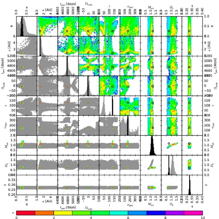
Figure 4: Constraints on the orbit of OGLE-2009-BLG-020L. The upper right-hand panels show the constraints from the Skowron et al. (2011) MCMC fit to the microlensing data. They are reproduced as the gray shaded regions in the lower left panels. The colored points in the lower left panels show the results of a joint MCMC to both the RV and microlensing data. The best joint fit is indicated by the black circle in the upper panels. The panels on the diagonal show the marginalized distributions of each parameter for the microlensing-only fit (gray) and the joint fit (black).

7 Conclusions

We have performed the first test of a microlensing detection of lens orbital motion by direct comparison of the microlensing orbit constraints to the measured orbital parameters from radial velocity observations of the lens system. Although the source and lens are not resolved, we show that the “contamination” of the lens spectrum by the source star is actually helpful. The fact that source is moving at constant radial velocity allows it to serve as a wavelength reference for our high-resolution spectra of the lens. We find that the orbit of OGLE-2009-BLG-020L as determined from radial velocity is fully consistent with the constraints from the microlensing light curve, which makes it the first confirmation of a microlensing measurement of orbital motion.

Demonstrating that the parameters of the microlensing solution are consistent with RV follow-up is a very strong confirmation of the method for including orbital motion in microlensing analysis. This test is completely independent of the microlensing data and is stronger than many previous tests of microlensing results because it constrains more parameters. Hence, we can now view the entire microlensing orbital motion sample and the parameters we have derived with more confidence, including in the case of planetary microlensing events for which such followup is not possible.

In the future, a stronger test should be possible for the microlens OGLE-2011-BLG-0417 (Gould et al., 2013; Shin et al., 2012). While the lens in this event is fainter, the microlensing constraints on the orbit are much better. In particular the form of the RV curve is predicted from the microlensing orbit measurement (see Figure 1 of Gould et al., 2013).

References

- Albrow et al. (2000) Albrow, M. D., Beaulieu, J.-P., Caldwell, J. A. R., et al. 2000, ApJ, 534, 894
- Alcock et al. (2000) Alcock, C., Allsman, R. A., Alves, D., et al. 2000, ApJ, 541, 270
- Alcock et al. (2001) Alcock, C., Allsman, R. A., Alves, D. R., et al. 2001, Nature, 414, 617
- Batista et al. (2011) Batista, V., Gould, A., Dieters, S., et al. 2011, A&A, 529, A102+
- Bennett et al. (2010) Bennett, D. P., Rhie, S. H., Nikolaev, S., et al. 2010, ApJ, 713, 837
- Bennett et al. (1999) Bennett, D. P., Rhie, S. H., Becker, A. C., et al. 1999, Nature, 402, 57
- Bernstein et al. (2003) Bernstein, R., Shectman, S. A., Gunnels, S. M., Mochnacki, S., & Athey, A. E. 2003, in Society of Photo-Optical Instrumentation Engineers (SPIE) Conference Series, Vol. 4841, Instrument Design and Performance for Optical/Infrared Ground-based Telescopes, ed. M. Iye & A. F. M. Moorwood, 1694–1704
- Dominik (1998) Dominik, M. 1998, A&A, 329, 361
- Dong et al. (2009) Dong, S., Gould, A., Udalski, A., et al. 2009, ApJ, 695, 970
- Eastman et al. (2013) Eastman, J., Gaudi, B. S., & Agol, E. 2013, PASP, 125, 83
- Einstein (1936) Einstein, A. 1936, Science, 84, 506
- Gould & Horne (2013) Gould, A., & Horne, K. 2013, ApJ, 779, L28
- Gould (1992) Gould, A. 1992, ApJ, 392, 442
- Gould et al. (2013) Gould, A., Shin, I.-G., Han, C., Udalski, A., & Yee, J. C. 2013, ApJ, 768, 126
- Gould (2004) —. 2004, ApJ, 606, 319
- Han & Gould (1995) Han, C., & Gould, A. 1995, ApJ, 449, 521
- Howard et al. (2010) Howard, A. W., Johnson, J. A., Marcy, G. W., et al. 2010, ApJ, 721, 1467
- Jung et al. (2013) Jung, Y. K., Han, C., Gould, A., & Maoz, D. 2013, ApJ, 768, L7
- Kelson (2003) Kelson, D. D. 2003, PASP, 115, 688
- Kelson et al. (2000) Kelson, D. D., Illingworth, G. D., van Dokkum, P. G., & Franx, M. 2000, ApJ, 531, 159
- Paczynski (1991) Paczynski, B. 1991, ApJ, 371, L63
- Pietrukowicz et al. (2005) Pietrukowicz, P., Kaluzny, J., Thompson, I. B., et al. 2005, Acta Astron., 55, 261
- Pietrukowicz et al. (2012) Pietrukowicz, P., Minniti, D., Jetzer, P., Alonso-García, J., & Udalski, A. 2012, ApJ, 744, L18
- Shin et al. (2011) Shin, I.-G., Udalski, A., Han, C., et al. 2011, ApJ, 735, 85
- Shin et al. (2012) Shin, I.-G., Han, C., Choi, J.-Y., et al. 2012, ApJ, 755, 91
- Skowron et al. (2011) Skowron, J., Udalski, A., Gould, A., et al. 2011, ApJ, 738, 87
- Udalski et al. (2005) Udalski, A., Jaroszyński, M., Paczyński, B., et al. 2005, ApJ, 628, L109
- Vogt et al. (1994) Vogt, S. S., Allen, S. L., Bigelow, B. C., et al. 1994, in Society of Photo-Optical Instrumentation Engineers (SPIE) Conference Series, Vol. 2198, Instrumentation in Astronomy VIII, ed. D. L. Crawford & E. R. Craine, 362
- Wright & Eastman (2014) Wright, J. T., & Eastman, J. D. 2014, PASP, 126, 838
- Yoo et al. (2004) Yoo, J., DePoy, D. L., Gal-Yam, A., et al. 2004, ApJ, 616, 1204
- Zucker (2003) Zucker, S. 2003, MNRAS, 342, 1291