Stress-driven solution to rate-independent
elasto-plasticity with damage at small strains
and its computer implementation.

Tomáš Roubíček
Mathematical Institute, Charles University, Sokolovská 83, CZ–186 75 Praha 8 and Institute of Thermomechanics, Czech Acad. Sci., Dolejškova 5, CZ–182 08 Praha 8 and Institute of Information Theory and Autom., Czech Acad. Sci., CZ–182 08 Praha 8, Czech Republic.

Jan Valdman
Institute of Information Theory and Automation, Czech Acad. Sci., Pod vodárenskou věží 4, CZ–182 08 Praha 8 and Institute of Mathematics and Biomathematics, Faculty of Science, University of South Bohemia, Branišovská 31, CZ–370 05 České Budějovice, Czech Republic.

1 INTRODUCTION

A combination of plasticity and damage, also called ductile damage, open colorful scenarios with important applications in civil or mechanical engineering and with interesting mathematical problems, in particular in comparison with mere plasticity or mere damage. Often, both plastification and damage processes are much faster than the rate of applied load and, in a basic scenario, any internal time scale is neglected and the mentioned inelastic processes are considered as rate independent. The goal of this article is to devise a model together with its efficient computational approximation that would lead to a numerical stable and convergent scheme and, at least in particular situations, calculate a physically relevant solutions of a stress-driven type verifiable aposteriori by checking a suitable version of the maximum-dissipation principle.

We use the very standard linearized, associative, plasticity at small strain as presented e.g. in [15]. Simultaneously, we use also a rather standard scalar (i.e. isotropic) damage as presented e.g. in [10]. We have primarily in mind a conventional engineering model with unidirectional evolution of damage; actually, the healing will be here allowed rather from analytical reasons and can be expected ineffective in usual applications, cf. Remark 2.1 below. All rate-dependent phenomena (as inertia or heat conduction and thermo-coupling) are neglected, this means the problem is considered as quasistatic and fully rate-independent. To avoid serious mathematical and computation difficulties, we have in mind an incomplete damage.

The mentioned modelling simplification leading to quasistatic rate-independent system however, which reflects a certain well-motivated asymptotics, brings however quite serious questions and difficulties because the class of reasonably general solutions is very wide if the governing energy is not convex (as necessarily here) and involves solutions of very different nature, some of them physically not relevant; cf. [20, 21]. In particular, to avoid unwanted effects of unphysically easy damage under subcritical stress, one cannot require (otherwise attractive idea of) energy conservation and thus cannot consider so-called energetic solutions in the sense [22], although this concept is occasionally used for damage with plasticity in purely mathematically-focused literature [2, 3, 9]. This is related with the discussion whether rather energy or rather stress is responsible for governing evolution of rate-independent systems [19].

In contrast to the mentioned energetic solutions (which allows for simpler analysis without considering gradient plasticity but lead to recursive global-minimization problems which are difficult to realize and may slide to unphysically scenarios of unrealistic early damage), we will focus here on solutions that are rather stress driven and that can be efficiently obtained numerically. We will rely on a certain careful usage of a suitable integral-version of the maximum-dissipation principle, as devised in [31] and used, rather heuristically, in engineering models of damage with plasticity and hardening, cf. [8]. This brings specific difficulties with convergence (which requires usage of gradient plasticity) and specific a-posteriori verification of a suitable approximate version of the mentioned maximum-dissipation principle, as suggested in [31, Rem. 4.6] for damage itself, modified here for the combination of damage and plasticity analogously like in [35] for a surface variant of the elasto-plasto-damage model. If the maximum-dissipation principle holds (at least with a good accuracy) we can claim that the numerically obtained solution is physically relevant as stress-driven (with a good accuracy).

A physically more justified and better motivated approach would be to involve a small viscosity to the damage variable or to the elastic and the plastic strains, and then to pass these viscosities to zero. The limits obtained by this way are called vanishing-viscosity solutions to the original rate-independent system and their analysis and computer implementation is very difficult; for models without plasticity cf. [17] for viscosity in damage or [34] for viscosity in elastic strain.

In principle, there are two basic scenarios how the material might respond to an increasing loading: either first plasticize and then go into damage due to hardening effects, or first go into damage and then plasticize; of course, various compromising scenarios are possible too. The latter scenario needs a damage influenced yield stress and allow for no hardening (and in particular perfect plasticity), cf. [36]. Let us only remark that a damage-dependence of the yield stress in the fully rate-independent setting would make the dissipation state-dependent, which brings serious difficulties as seen e.g. in [21, Sect. 3.2] and, for the particular elasto-plasto-damage model, in [2, 3, 9]. In this paper, we will however concern exclusively on the former scenario, i.e. in particular, the damage does not influence the yield stress. Moreover, we will consider only kinematic hardening, although all the considerations could easily be augmented by isotropic hardening, too. (Another essential difference from [36] is that, as already explained, the energy is intentionally not conserved in here.)

The plan of the paper is as follows: In Section 2 we devise the model in its classical formulation and then, in Section 3, its suitable weak formulation with discussing stress-driven solutions and the role of the maximum-dissipation principle. In Section 4, we propose a constructive time discretisation method and prove its numerical stability (i.e. a-priori estimates) and convergence towards weak solutions. After a further finite-element discretisation outlined in Section 5, this allows for efficient computer implementation of the model, which is demonstrated on illustrative 2-dimensional examples in Section 6.

2 THE MODEL AND ITS WEAK FORMULATION

Hereafter, we suppose that the damageable elasto-plastic body occupies a bounded Lipschitz domain $\Omega\subset{\mathbb{R}}^{d}$, $d=2$ or $3$. We denote by $\vec{n}$ the outward unit normal to $\partial\Omega$. We further suppose that the boundary of $\Omega$ splits as

$$\partial\Omega:=\Gamma=\mathchoice{\Gamma_{\mbox{\tiny\rm D}}}{\Gamma_{\mbox{\tiny\rm D}}}{\Gamma_{\mbox{\tiny\rm D}}}{\Gamma_{\mbox{\tiny\rm D}}}\cup\Gamma_{\mbox{\tiny\rm N}}\,,$$

with $\mathchoice{\Gamma_{\mbox{\tiny\rm D}}}{\Gamma_{\mbox{\tiny\rm D}}}{\Gamma_{\mbox{\tiny\rm D}}}{\Gamma_{\mbox{\tiny\rm D}}}$ and $\Gamma_{\mbox{\tiny\rm N}}$ open subsets in the relative topology of $\partial\Omega$, disjoint one from each other and, up to $(d{-}1)$-dimensional zero measure, covering $\partial\Omega$. Later, the Dirichlet or the Neumann boundary conditions will be prescribed on $\mathchoice{\Gamma_{\mbox{\tiny\rm D}}}{\Gamma_{\mbox{\tiny\rm D}}}{\Gamma_{\mbox{\tiny\rm D}}}{\Gamma_{\mbox{\tiny\rm D}}}$ and $\Gamma_{\mbox{\tiny\rm N}}$, respectively. Considering $T>0$ a fixed time horizon, we set

$$I:=[0,T],\qquad Q:=(0,T){\times}\Omega,\qquad\Sigma:=I{\times}\Gamma,\qquad\Sigma_{\mbox{\tiny\rm D}}\!:=I{\times}\mathchoice{\Gamma_{\mbox{\tiny\rm D}}}{\Gamma_{\mbox{\tiny\rm D}}}{\Gamma_{\mbox{\tiny\rm D}}}{\Gamma_{\mbox{\tiny\rm D}}},\qquad\Sigma_{\mbox{\tiny\rm N}}\!:=I{\times}\Gamma_{\mbox{\tiny\rm N}}.$$

Further, ${\mathbb{R}}_{\mathrm{sym}}^{d\times d}$ and ${\mathbb{R}}_{\mathrm{dev}}^{d\times d}$ will denote the set of symmetric or symmetric trace-free (= deviatoric) $(d{\times}d)$-matrices, respectively. For readers’ convenience, let us summarize the basic notation used in what follows:

$d=2,3$ dimension of the problem, ${\mathbb{R}}_{\mathrm{sym}}^{d\times d}:=\{A\in{\mathbb{R}}^{d\times d};\ A=A^{\top}\}$, ${\mathbb{R}}_{\mathrm{dev}}^{d\times d}:=\{A\in{\mathbb{R}}_{\mathrm{sym}}^{d\times d};\ \mathrm{tr}\,A=0\}$, $u:Q\to{\mathbb{R}}^{d}$ displacement, $\pi:Q\to{\mathbb{R}}_{\mathrm{dev}}^{d\times d}$ plastic strain, $\zeta:Q\to[0,1]$ damage variable, $a>0$ activation energy for damage, $f{:}\Sigma_{\mbox{\tiny\rm N}}\to{\mathbb{R}}^{d}$ applied traction force, $g{:}Q\to{\mathbb{R}}^{d}$ applied bulk force (as gravity), $\sigma_{\mathrm{el}}:Q\to{\mathbb{R}}_{\mathrm{sym}}^{d\times d}$ elastic stress,    $e_{\mathrm{el}}:Q\to{\mathbb{R}}_{\mathrm{sym}}^{d\times d}$ elastic strain, $e=e(u)=e_{\mathrm{el}}{+}\pi=\frac{1}{2}\nabla u^{\top}\!+\frac{1}{2}\nabla u$ total small-strain tensor, $\mathbb{C}:[0,1]\to{\mathbb{R}}^{3^{4}}$ elasticity tensor (dependent on $\zeta$), $\mathbb{H}\in{\mathbb{R}}^{3^{4}}$ hardening tensor (independent of $\zeta$) $S\subset{\mathbb{R}}_{\mathrm{dev}}^{d\times d}$ the elastic domain (convex, int $S\ni 0$), $w_{\mbox{\tiny\rm D}}:\Sigma_{\mbox{\tiny\rm D}}\to{\mathbb{R}}^{d}$ prescribed boundary displacement, $\kappa_{1}>0$ scale coefficient of the gradient of plasticity, $\kappa_{2}>0$ scale coefficient of the gradient of damage, $b>0$ activation energy for possible healing.

Table 1.  Summary of the basic notation used through the paper.

The state is formed by the triple $q:=(u,\pi,\zeta)$. Considering still a (small but fixed) regularizing parameter $\varepsilon>0$, the governing equation/inclusions read as:

$$\mathrm{div}\,\sigma_{\mathrm{el}}+g=0\ \ \ \text{ with }\ \sigma_{\mathrm{el}}=\mathbb{C}(\zeta)e_{\mathrm{el}}\ \text{ and }\ e_{\mathrm{el}}=e(u){-}\pi,$$ (momentum equilibrium) (2.1a)

$$\partial\delta_{S}^{*}(\mathchoice{{\buildrel\hskip 1.00006pt\text{\LARGE.}\over{\pi}}}{{\buildrel\hskip 1.00006pt\text{\Large.}\over{\pi}}}{{\buildrel\hskip 1.00006pt\text{\large.}\over{\pi}}}{{\buildrel\hskip 1.00006pt\text{\large.}\over{\pi}}})\ni\mathrm{dev}\,\sigma_{\mathrm{el}}-\mathbb{H}\pi+\kappa_{1}\Delta\pi,$$ (plastic flow rule) (2.1b)

$$\partial\delta_{[-a,b]}^{*}(\mathchoice{{\buildrel\hskip 1.00006pt\text{\LARGE.}\over{\zeta}}}{{\buildrel\hskip 1.00006pt\text{\Large.}\over{\zeta}}}{{\buildrel\hskip 1.00006pt\text{\large.}\over{\zeta}}}{{\buildrel\hskip 1.00006pt\text{\large.}\over{\zeta}}})\ni-\frac{1}{2}\mathbb{C}^{\prime}(\zeta)e_{\mathrm{el}}:e_{\mathrm{el}}+\kappa_{2}\,\mathrm{div}\big{(}|\nabla\zeta|^{r-2}\nabla\zeta\big{)}-N_{[0,1]}(\zeta),$$ (damage flow rule) (2.1c)

with $\delta_{S}$ the indicator function to $S$ and $\delta_{S}^{*}$ its convex conjugate and with “$\operatorname*{dev}$” denoting the deviatoric part of a tensor, i.e. $\operatorname*{dev}\,A:=A-\mathrm{tr}\,A/d$. Here, $[\mathbb{C}(\zeta)e]_{ij}$ means $\sum_{k,l=1}^{d}\mathbb{C}_{ijkl}(\zeta)e_{kl}$.

We employed the regularizing term with a regularizing parameter $\varepsilon>0$ with an exponent to be assumed suitably big, namely $r>d$. This regularization will facilitate analytical well-posedness of the problem and, because the gradient-damage term degenerates at $\nabla\zeta=0$, its influence is presumably small if $\varepsilon$ is small and $\nabla\zeta$ not too large.

Of course, (2.1) is to be completed by appropriate boundary conditions, e.g.

$$u=w_{\mbox{\tiny\rm D}} \text{on }\mathchoice{\Gamma_{\mbox{\tiny\rm D}}}{\Gamma_{\mbox{\tiny\rm D}}}{\Gamma_{\mbox{\tiny\rm D}}}{\Gamma_{\mbox{\tiny\rm D}}},$$ (2.2a)

$$\sigma_{\mathrm{el}}{\cdot}\vec{n}=f \text{on }\Gamma_{\mbox{\tiny\rm N}},$$ (2.2b)

$$\nabla\pi\vec{n}=0\ \ \text{ and }\ \ \nabla\zeta{\cdot}\vec{n}=0 \text{on }\Gamma$$ (2.2c)

with $\vec{n}$ denoting the unit outward normal to $\Omega$. We will consider an initial-value problem for (2.1)–(2.2) by asking for

$$u(0)=u_{0},\ \ \ \ \ \pi(0)=\pi_{0},\ \ \text{ and }\ \ \zeta(0)=\zeta_{0}.$$ (2.3)

In fact, as $\mathchoice{{\buildrel\hskip 1.00006pt\text{\LARGE.}\over{u}}}{{\buildrel\hskip 1.00006pt\text{\Large.}\over{u}}}{{\buildrel\hskip 1.00006pt\text{\large.}\over{u}}}{{\buildrel\hskip 1.00006pt\text{\large.}\over{u}}}$ does not occur in (2.1), $u_{0}$ is rather formal and its only qualification is to make $\mathscr{E}(0,u_{0},\pi_{0},\zeta_{0})$ finite not to degrade the energy balance (3.1d) on $[0,t]$.

After considering an extension $u_{\mbox{\tiny\rm D}}=u_{\mbox{\tiny\rm D}}(t)$ of $w_{\mbox{\tiny\rm D}}(t)$ from (2.2a) on the whole domain $\Omega$, it is convenient to make a substitution of $u+u_{\mbox{\tiny\rm D}}$ instead of $u$ into (2.1)–(2.2), we arrive to the problem with time-constant (even homogeneous) Dirichlet boundary conditions. More specifically,

$$e_{\mathrm{el}}\ \,\text{ in \eqref{plast-dam12} replaces by }\ e_{\mathrm{el}}=e(u{+}u_{\mbox{\tiny\rm D}}){-}\pi,\ \text{ and}$$ (2.4a)

$$w_{\mbox{\tiny\rm D}}\ \text{ in \eqref{plast-dam-BC1} replaces by }0.$$ (2.4b)

Assuming $(\mathbb{C}(\zeta)e(u_{\mbox{\tiny\rm D}}){\cdot}\vec{n}=0$ on $\Gamma_{\mbox{\tiny\rm N}}$ for any admissible $\zeta$, this transformation will keep $f$ in (2.2b) unchanged.

Actually, (2.1b) represents rather the thermodynamical-force balance governing damage evolution while the corresponding flow rule is written rather in the (equivalent) form

$$\mathchoice{{\buildrel\hskip 1.00006pt\text{\LARGE.}\over{\pi}}}{{\buildrel\hskip 1.00006pt\text{\Large.}\over{\pi}}}{{\buildrel\hskip 1.00006pt\text{\large.}\over{\pi}}}{{\buildrel\hskip 1.00006pt\text{\large.}\over{\pi}}}\in N_{S}\big{(}\mathrm{dev}\,\sigma_{\mathrm{el}}-\mathbb{H}\pi-\kappa_{1}\Delta\pi\big{)}\ \ \ \text{ with }\ \sigma_{\mathrm{el}}=\mathbb{C}(\zeta)e_{\mathrm{el}}$$ (2.5)

and with $N_{S}$ denoting the set-valued normal-cone mapping to the convex set $S$. An analogous remark applies to (2.1c). The system (2.1) with the boundary conditions (2.2) has, in its weak formulation, the structure of an abstract Biot-type equation (or here rather inclusion, cf. also e.g. [4, 21, 24]):

$$\partial_{\mathchoice{{\buildrel\hskip 0.70004pt\text{\LARGE.}\over{q}}}{{\buildrel\hskip 0.70004pt\text{\Large.}\over{q}}}{{\buildrel\hskip 0.70004pt\text{\large.}\over{q}}}{{\buildrel\hskip 0.70004pt\text{\large.}\over{q}}}}\mathscr{R}(\mathchoice{{\buildrel\hskip 1.00006pt\text{\LARGE.}\over{q}}}{{\buildrel\hskip 1.00006pt\text{\Large.}\over{q}}}{{\buildrel\hskip 1.00006pt\text{\large.}\over{q}}}{{\buildrel\hskip 1.00006pt\text{\large.}\over{q}}})+\partial_{q}\mathscr{E}(t,q)\ni 0$$ (2.6)

with suitable time-dependent stored-energy functional $\mathscr{E}$ and the state-dependent (pseudo))potential of dissipative forces $\mathscr{R}$. Equally, as already used in (2.5), one can write (2.6) as a generalized gradient flow

$$\mathchoice{{\buildrel\hskip 1.00006pt\text{\LARGE.}\over{q}}}{{\buildrel\hskip 1.00006pt\text{\Large.}\over{q}}}{{\buildrel\hskip 1.00006pt\text{\large.}\over{q}}}{{\buildrel\hskip 1.00006pt\text{\large.}\over{q}}}\in\partial_{\xi}\mathscr{R}^{*}\big{(}-\partial\mathscr{E}(t,q)\big{)}$$ (2.7)

where $\mathscr{R}^{*}$ denotes the conjugate functional. The governing functionals corresponding to (2.1)–(2.2) after the transformation (2.4) are:

$$\mathscr{E}(t,u,\pi,\zeta):=\int_{\Omega}\!\frac{1}{2}\mathbb{C}(\zeta)\big{(}e(u{+}u_{\mbox{\tiny\rm D}}(t)){-}\pi\big{)}:\big{(}e(u{+}u_{\mbox{\tiny\rm D}}(t)){-}\pi\big{)}+\frac{1}{2}\mathbb{H}\pi:\pi$$

$$\hskip 80.00012pt+\frac{\kappa_{1}}{2}|\nabla\pi|^{2}\!+\frac{\kappa_{2}}{r}|\nabla\zeta|^{r}\!+\delta_{[0,1]}(\zeta)-g(t){\cdot}u\,\mathrm{d}x-\int_{\Gamma_{\mbox{\tiny\rm N}}}\!f(t){\cdot}u\,\mathrm{d}S,$$ (2.8a)

$$\mathscr{R}(\mathchoice{{\buildrel\hskip 1.00006pt\text{\LARGE.}\over{\pi}}}{{\buildrel\hskip 1.00006pt\text{\Large.}\over{\pi}}}{{\buildrel\hskip 1.00006pt\text{\large.}\over{\pi}}}{{\buildrel\hskip 1.00006pt\text{\large.}\over{\pi}}},\mathchoice{{\buildrel\hskip 1.00006pt\text{\LARGE.}\over{\zeta}}}{{\buildrel\hskip 1.00006pt\text{\Large.}\over{\zeta}}}{{\buildrel\hskip 1.00006pt\text{\large.}\over{\zeta}}}{{\buildrel\hskip 1.00006pt\text{\large.}\over{\zeta}}})\equiv\mathscr{R}_{1}(\mathchoice{{\buildrel\hskip 1.00006pt\text{\LARGE.}\over{\pi}}}{{\buildrel\hskip 1.00006pt\text{\Large.}\over{\pi}}}{{\buildrel\hskip 1.00006pt\text{\large.}\over{\pi}}}{{\buildrel\hskip 1.00006pt\text{\large.}\over{\pi}}})+\mathscr{R}_{2}(\mathchoice{{\buildrel\hskip 1.00006pt\text{\LARGE.}\over{\zeta}}}{{\buildrel\hskip 1.00006pt\text{\Large.}\over{\zeta}}}{{\buildrel\hskip 1.00006pt\text{\large.}\over{\zeta}}}{{\buildrel\hskip 1.00006pt\text{\large.}\over{\zeta}}}):=\int_{\Omega}\delta_{S}^{*}(\mathchoice{{\buildrel\hskip 1.00006pt\text{\LARGE.}\over{\pi}}}{{\buildrel\hskip 1.00006pt\text{\Large.}\over{\pi}}}{{\buildrel\hskip 1.00006pt\text{\large.}\over{\pi}}}{{\buildrel\hskip 1.00006pt\text{\large.}\over{\pi}}})+a\mathchoice{{\buildrel\hskip 1.00006pt\text{\LARGE.}\over{\zeta}}}{{\buildrel\hskip 1.00006pt\text{\Large.}\over{\zeta}}}{{\buildrel\hskip 1.00006pt\text{\large.}\over{\zeta}}}{{\buildrel\hskip 1.00006pt\text{\large.}\over{\zeta}}}^{-}+b\mathchoice{{\buildrel\hskip 1.00006pt\text{\LARGE.}\over{\zeta}}}{{\buildrel\hskip 1.00006pt\text{\Large.}\over{\zeta}}}{{\buildrel\hskip 1.00006pt\text{\large.}\over{\zeta}}}{{\buildrel\hskip 1.00006pt\text{\large.}\over{\zeta}}}^{+}\,\mathrm{d}x$$ (2.8b)

where $z^{+}:=\max(z,0)$ and $z^{-}:=\max(-z,0)\geq 0$. Note that the damage does not affect the hardening, which reflects the idea that, on the microscopical level, damage in the material that underwent hardening develops by evolving microcracks and even a completely damaged material consists of micro-pieces that bear the hardening energy $\frac{1}{2}\mathbb{H}\pi:\pi$ stored before. This model preserves coercivity of hardening even under a complete damage but the analysis below admits only incomplete damage. If $\zeta\mapsto\mathbb{C}(\zeta)e{:}e$ is strictly convex for any $e\neq 0$, we speak about a cohesive damage which exhibits a certain hardening effect so that the needed driving force increases when damage is to be accomplished. We can thus model quite a realistic response to various loading experiments, as schematically shown on Figure 1 for the case of a possible complete damage (whose analysis remains open, however). Note that, due to the “incompressibility” constraint $\operatorname*{tr}\,\pi=0$, no plastification is triggered under a pure tension or compression loading.

\psfrag{TENSION/COMPRESSION}{\small\bf TENSION/COMPRESSION}\psfrag{SHEAR LOADING}{\small\bf SHEAR LOADING}\psfrag{[u]t}{\footnotesize$e=e(u)$}\psfrag{elasticity}{\footnotesize elasticity}\psfrag{damage}{\footnotesize damage}\psfrag{plasticity}{\footnotesize plasticity with hardening}\psfrag{stress2}{\footnotesize$\sigma_{\mathrm{el}}$}\psfrag{sd}{\footnotesize$\displaystyle{\!\sqrt{\frac{2a}{C^{\prime}(1)}}C(1)}$}\psfrag{sd2}{\footnotesize$|S|$}\psfrag{s2}{\footnotesize$|S|/|C(1)|$}\psfrag{e3}{\footnotesize$\displaystyle{e=\sqrt{\frac{2a}{|C^{\prime}(0)|}}}$}\psfrag{e4}{\footnotesize$\displaystyle{e=\sqrt{\frac{2a}{|C^{\prime}(1)|}}}$}\psfrag{slope}{\footnotesize\!slope\,=\,$C(1)$}\psfrag{slope2}{\footnotesize slope\,=\,$\displaystyle{\frac{C(1)H}{C(1){+}H}}$}\includegraphics[width=399.05275pt]{tr-plast-dam.eps}

Figure 1: Schematic response of the stress $\sigma_{\mathrm{el}}$ to the total strain $e$ during a “one-dimensional” tension (left) or shear (right) loading experiment under a stress-driven scenario. The latter option combines plasticity with eventual complete damage. Dashed lines outline a response to unloading, $C=C(\zeta)$ refers to Young’s modulus (left) or the shear modulus (right).

Let us further note that $(u,\pi)\mapsto\mathscr{E}(t,u,\pi,\zeta)$ is smooth so that $\partial_{q}\mathscr{E}=\{\mathscr{E}_{u}^{\prime}\}\times\{\mathscr{E}_{\pi}^{\prime}\}\times\partial_{\zeta}\mathscr{E}$ with $\mathscr{E}_{u}^{\prime}$ and $\mathscr{E}_{\pi}^{\prime}$ denoting the respective partial Gâteaux derivatives and (2.6) can thus be written more specifically as the system:

$$\mathscr{E}_{u}^{\prime}(t,u,\pi,\zeta) =0,$$ (2.9a)

$$\partial\mathscr{R}_{1}(\mathchoice{{\buildrel\hskip 1.00006pt\text{\LARGE.}\over{\pi}}}{{\buildrel\hskip 1.00006pt\text{\Large.}\over{\pi}}}{{\buildrel\hskip 1.00006pt\text{\large.}\over{\pi}}}{{\buildrel\hskip 1.00006pt\text{\large.}\over{\pi}}})+\mathscr{E}_{\pi}^{\prime}(t,u,\pi,\zeta) \,\ni\,0,$$ (2.9b)

$$\partial\mathscr{R}_{2}(\mathchoice{{\buildrel\hskip 1.00006pt\text{\LARGE.}\over{\zeta}}}{{\buildrel\hskip 1.00006pt\text{\Large.}\over{\zeta}}}{{\buildrel\hskip 1.00006pt\text{\large.}\over{\zeta}}}{{\buildrel\hskip 1.00006pt\text{\large.}\over{\zeta}}})+\partial_{\zeta}\mathscr{E}(t,u,\pi,\zeta) \,\ni\,0.$$ (2.9c)

Remark 2.1 (Irreversible damage in engineering models).

Usual engineering models consider $b=\infty$, i.e. no healing is allowed. In fact, due to an essentially missing driving force for healing, our modification $b<\infty$ would not have any influence on the evolution if it were not any $\nabla\zeta$-term in the stored energy. Thus, if the healing threshold $b$ is big and the gradient-term coefficient $\kappa_{2}>0$ is small, we expect to have essentially the (usually desired) unidirectional evolution as far as the damage concerns.

Remark 2.2 (Surface variant of the damage/plasticity).

A similar scenario distinguishing tension (which leads to damage without plastification) and shear (with plastifying the material before damage) as in Figure 1 was used in a surface variant to model an adhesive contact distinguishing delamination in the opening and in the shearing modes, devised in [32, 33] and later implemented by the fractional-step discretisation with checking the approximate maximum-dissipation principle in [25, 35, 42]. An additional analytical difference is that, in contrast to our bulk model here, the surface variant allows for irreversible damage that does not need any gradient.

Remark 2.3 (Other material models).

A separately convex stored energy $\mathscr{E}(t,\cdot)$ occurs also in other models. E.g., some phenomenological models for phase transformations in (polycrystalline) shape-memory materials [37] gives $\zeta$ the meaning of a volume fraction (instead of damage) and $\pi$ a transformation strain (or a combination of the plastic and the transformation strains), and the total strain decomposes as $e(u)=e_{\rm el}+\zeta\pi$ rather than (2.1a) or makes $\pi$ dependent on $\zeta$ (which is then vector-valued). Considering the degree-1 homogeneous dissipation potential, most of the considerations in this paper can be applied to such a model, too; in fact, the only difference would be the nonsmoothness of $\mathscr{E}$ also with respect to $\pi$ variable. A similar (in general non-convex) model have been also considered in [5, 11, 18, 22, 38] although sometimes special choices of elastic moduli leading to convex were particularly under focus while the dissipation is made state-dependent.

3 LOCAL SOLUTIONS

We will use the standard notation $W^{1,p}(\Omega)$ for the Sobolev space of functions having the gradient in the Lebesgue space $L^{p}(\Omega;{\mathbb{R}}^{d})$. If valued in ${\mathbb{R}}^{n}$ with $n\geq 2$, we will write $W^{1,p}(\Omega;{\mathbb{R}}^{n})$, and furthermore we use the shorthand notation $H^{1}(\Omega;{\mathbb{R}}^{n})=W^{1,2}(\Omega;{\mathbb{R}}^{n})$. We also use the notation of “$\,\cdot\,$” and “$\,:\,$” for a scalar product of vectors and 2nd-order tensors, respectively, and later also “   ^⋮   ” for 3rd-order tensors. For a Banach space $X$, $L^{p}(I;X)$ will denote the Bochner space of $X$-valued Bochner measurable functions $u:I\to X$ with its norm $\|u(\cdot)\|$ in $L^{p}(I)$, here $\|\cdot\|$ stands for the norm in $X$. Further, $W^{1,p}(I;X)$ denotes the Banach space of mappings $u:I\to X$ whose distributional time derivative is in $L^{p}(I;X)$, while ${\rm BV}(I;X)$ will denote the space of mappings $u:I\to X$ with a bounded variations, i.e. $\sup_{0\leq t_{0}<t_{1}<...<t_{n-1}<t_{n}\leq T}\sum_{i=1}^{n}\|u(t_{i}){-}u(t_{i-1})\|<\infty$ where the supremum is taken over all finite partitions of the interval $I=[0,T]$. By ${\rm B}(I;X)$ we denote the space of bounded measurable (everywhere defined) mappings $I\to X$.

The concept of local solutions has been introduced for a special crack problem in [40] and independently also in [39], and further generally investigated in [20]. Here, we additionally combine it with the concept of semi-stability as invented in [29]. We adapt the general definition directly to our specific problem, which will lead to two semi-stability conditions for $\zeta$ and $\pi$, respectively:

Definition 3.1 (Local solutions).

We call a measurable mapping $(u,\pi,\zeta):I\to H^{1}(\Omega;{\mathbb{R}}^{d})\times H^{1}(\Omega;{\mathbb{R}}_{\mathrm{dev}}^{d\times d})\times W^{1,r}(\Omega)$ a local solution to the elasto-plasto-damage problem (2.1)–(2.3) if the initial conditions (2.3) are satisfied and, for some $J\subset I$ at most countable (containing time instances where the solution may possibly jump), it holds that:

$$\!\!\!\forall t\!\in\!I{\setminus}J:\ \ \ \mathscr{E}_{u}^{\prime}\big{(}t,u(t),\pi(t),\zeta(t)\big{)}=0,$$ (3.1a)

$$\!\!\!\forall t\!\in\!I{\setminus}J\ \forall\widetilde{\pi}\!\in\!H^{1}(\Omega;{\mathbb{R}}_{\mathrm{dev}}^{d\times d}):\ \mathscr{E}\big{(}t,u(t),\pi(t),\zeta(t)\big{)}\leq\mathscr{E}\big{(}t,u(t),\widetilde{\pi},\zeta(t)\big{)}+\mathscr{R}_{1}\big{(}\widetilde{\pi}{-}\pi(t)\big{)},$$ (3.1b)

$$\!\!\!\forall t\!\in\!I{\setminus}\{0\}\ \forall\widetilde{\zeta}\!\in\!W^{1,r}(\Omega),\ \,0\!\leq\!\widetilde{\zeta}\!\leq\!1:\ \$$

$$\qquad\qquad\qquad\quad\ \mathscr{E}\big{(}t,u(t),\pi(t),\zeta(t)\big{)}\leq\mathscr{E}\big{(}t,u(t),\pi(t),\widetilde{\zeta}\big{)}+\mathscr{R}_{2}\big{(}\widetilde{\zeta}{-}\zeta(t)\big{)},$$ (3.1c)

$$\!\!\!\forall 0\!\leq\!t_{1}\!\leq\!t_{2}\!\leq\!T:\ \ \,\mathscr{E}\big{(}t_{2},u(t_{2}),\pi(t_{2}),\zeta(t_{2})\big{)}+{\rm Diss}_{\mathscr{R}_{1}}\big{(}\pi;[t_{1},t_{2}]\big{)}+{\rm Diss}_{\mathscr{R}_{2}}\big{(}\zeta;[t_{1},t_{2}]\big{)}$$

$$\hskip 110.00017pt\leq\mathscr{E}\big{(}t_{1},u(t_{1}),\pi(t_{1}),\zeta(t_{1})\big{)}+\!\int_{t_{1}}^{t_{2}}\!\!\mathscr{E}_{t}^{\prime}(t,u(t),\pi(t),\zeta(t))\,\mathrm{d}t,$$ (3.1d)

where

$$\mathrm{Diss}_{\mathscr{R}_{1}}(\pi;[r,s]):=\!\!\!\!\sup_{\begin{subarray}{c}N\in{\mathbb{N}}\\[0.70004pt] r\leq t_{0}<t_{1}<\cdots<t_{N-1}<t_{N}\leq s\end{subarray}}\sum_{j=1}^{N}\int_{\Omega}\delta_{S}^{*}(\pi(t_{j-1}){-}\pi(t_{j}))\,\mathrm{d}x,\ \ \ \text{ and similarly }$$ (3.2a)

$$\mathrm{Diss}_{\mathscr{R}_{2}}(\zeta;[r,s]):=\!\!\!\!\sup_{\begin{subarray}{c}N\in{\mathbb{N}}\\[0.70004pt] r\leq t_{0}<t_{1}<\cdots<t_{N-1}<t_{N}\leq s\end{subarray}}\sum_{j=1}^{N}\int_{\Omega}a(\pi(t_{j-1}){-}\pi(t_{j}))^{-}+b(\pi(t_{j-1}){-}\pi(t_{j}))^{+}\,\mathrm{d}x.$$

Let us comment the above definition briefly. Obviously, (2.1a) after transforming the boundary condition (2.4) means precisely (3.1a), which more in detail here means that $\int_{\Omega}\mathbb{C}(\zeta(t))(e(u(t){-}w_{\mbox{\tiny\rm D}}(t))-\pi){:}e(v)\,\mathrm{d}x=\int_{\Omega}g{\cdot}v\,\mathrm{d}x+\int_{\Gamma_{\mbox{\tiny\rm N}}}f{\cdot}v\,\mathrm{d}S$ for all $v\!\in\!H^{1}(\Omega;{\mathbb{R}}^{d})$ with $v|_{\mathchoice{\Gamma_{\mbox{\tiny\rm D}}}{\Gamma_{\mbox{\tiny\rm D}}}{\Gamma_{\mbox{\tiny\rm D}}}{\Gamma_{\mbox{\tiny\rm D}}}}=0$, i.e. the weakly formulated Euler-Lagrange equation for displacement. Note that (3.1a) specifies also the boundary conditions for $u$, namely $u=0$ on $\mathchoice{\Gamma_{\mbox{\tiny\rm D}}}{\Gamma_{\mbox{\tiny\rm D}}}{\Gamma_{\mbox{\tiny\rm D}}}{\Gamma_{\mbox{\tiny\rm D}}}$ because otherwise $\mathscr{E}(t,u,\pi,\zeta)=\infty$ would violate (3.1a) for $v$ which satisfies $v=0$ on $\mathchoice{\Gamma_{\mbox{\tiny\rm D}}}{\Gamma_{\mbox{\tiny\rm D}}}{\Gamma_{\mbox{\tiny\rm D}}}{\Gamma_{\mbox{\tiny\rm D}}}$, and also $\sigma_{\rm el}\cdot\vec{n}=f$ on $\Gamma_{\mbox{\tiny\rm N}}$ can be proved by standard arguments based on Green’s theorem. Equivalently, one can merge (3.1a) with (3.1b) to a single condition

$$\!\!\!\forall t\!\in\!I{\setminus}J\ \forall(\widetilde{u},\widetilde{\pi})\!\in\!H^{1}(\Omega;{\mathbb{R}}^{d})\times H^{1}(\Omega;{\mathbb{R}}_{\mathrm{dev}}^{d\times d}),\ \ \widetilde{u}|_{\mathchoice{\Gamma_{\mbox{\tiny\rm D}}}{\Gamma_{\mbox{\tiny\rm D}}}{\Gamma_{\mbox{\tiny\rm D}}}{\Gamma_{\mbox{\tiny\rm D}}}}=0:\quad$$

$$\qquad\qquad\qquad\qquad\qquad\qquad\quad\mathscr{E}\big{(}t,u(t),\pi(t),\zeta(t)\big{)}\leq\mathscr{E}\big{(}t,\widetilde{u},\widetilde{\pi},\zeta(t)\big{)}+\mathscr{R}_{1}\big{(}\widetilde{\pi}{-}\pi(t)\big{)};$$ (3.3)

which reveals that Definition 3.1 just copies the concept of local solutions from [39, 40] here generalized for the case of non-vanishing dissipation $\mathscr{R}_{1}\neq 0$. As $\mathscr{R}_{1}$ is homogeneous degree-1, always $\partial\mathscr{R}_{1}(\mathchoice{{\buildrel\hskip 1.00006pt\text{\LARGE.}\over{\pi}}}{{\buildrel\hskip 1.00006pt\text{\Large.}\over{\pi}}}{{\buildrel\hskip 1.00006pt\text{\large.}\over{\pi}}}{{\buildrel\hskip 1.00006pt\text{\large.}\over{\pi}}})\subset\partial\mathscr{R}_{1}(0)$ and thus (2.9b) implies $\partial\mathscr{R}_{1}(0)+\partial_{\pi}\mathscr{E}(u,\pi,\zeta)\ni 0$. From the convexity of $\mathscr{R}_{1}$ when taking into account that $\mathscr{R}_{1}(0)=0$, the latter inclusion is equivalent to $\mathscr{R}_{1}(v)+\langle\partial_{\pi}\mathscr{E}(u(t),\pi(t),\zeta(t)),v\rangle\geq 0$ for any $v\in H^{1}(\Omega;{\mathbb{R}}_{\mathrm{dev}}^{d\times d})$. Substituting $v=\widetilde{z}-z(t)$ and using the convexity of $\mathscr{E}(t,u,\zeta,\cdot)$, we obtain the semi-stability (3.1b) of $\pi$ at time $t$. Analogously, we obtain also (3.1c) from (2.9c); note that we do not require its validity at $t=0$ so that we do not need to qualify the initial conditions as far as any (semi)stability concerns. Eventually, (3.1d) is the (im)balance of the mechanical energy. Note that, in view of (2.8a), the last term in (4.12d) involves

$$\mathscr{E}_{t}^{\prime}(t,u,\pi,\zeta)=\int_{\Omega}\!\mathbb{C}(\zeta)\big{(}e(\mathchoice{{\buildrel\hskip 1.00006pt\text{\LARGE.}\over{u}}}{{\buildrel\hskip 1.00006pt\text{\Large.}\over{u}}}{{\buildrel\hskip 1.00006pt\text{\large.}\over{u}}}{{\buildrel\hskip 1.00006pt\text{\large.}\over{u}}}_{\mbox{\tiny\rm D}})\big{)}:\big{(}e(u{+}u_{\mbox{\tiny\rm D}}){-}\pi\big{)}-\mathchoice{{\buildrel\hskip 1.00006pt\text{\LARGE.}\over{g}}}{{\buildrel\hskip 1.00006pt\text{\Large.}\over{g}}}{{\buildrel\hskip 1.00006pt\text{\large.}\over{g}}}{{\buildrel\hskip 1.00006pt\text{\large.}\over{g}}}(t){\cdot}u\,\mathrm{d}x-\int_{\Gamma_{\mbox{\tiny\rm N}}}\!\!\mathchoice{{\buildrel\hskip 1.00006pt\text{\LARGE.}\over{f}}}{{\buildrel\hskip 1.00006pt\text{\Large.}\over{f}}}{{\buildrel\hskip 1.00006pt\text{\large.}\over{f}}}{{\buildrel\hskip 1.00006pt\text{\large.}\over{f}}}(t){\cdot}u\,\mathrm{d}S.$$

This is equivalent (or, if $\mathscr{E}(t,\cdot,\cdot,\cdot)$ is not smooth, slightly generalizes) the standard definition of the weak solution to the initial-boundary-value problem (2.1)–(2.3), cf. [31, Prop. 2.3] for details.

To be more precise, the concept of local solutions as used in [20, 40] requires $J$ only to have a zero Lebesgue measure and also (3.1c) is valid only for a.a. $t$. On the other hand, conventional weak solutions allow even (3.1d) holding only for a.a. $t_{1}$ and $t_{2}$. Later, our approximation method will provide convergence to this slightly stronger local solutions, which motivates us to have tailored Definition 3.1 straight to our results.

Actually, local solutions form essentially the largest reasonable class of solutions for rate-independent systems as (2.1)–(2.3) considered here. It includes the mentioned energetic solutions [20, 22], the vanishing-viscosity solutions, the balanced-viscosity (so-called BV) solutions, parametrized solutions, etc.; cf. [20, 21] for a survey, and also stress-driven-like solutions obeying maximum-dissipation principle in some sense, cf. Remark 3.2. The energetic solutions have often tendency to undergo damage unphysically early; cf. [42] for a comparison on several computational experiments on a similar type of problem. The approximation method we will use in this article leads rather to the stress-driven option, cf. Remarks 3.2 and 4.3 below.

Remark 3.2 (Maximum-dissipation principle).

The degree-1 homogeneity of $\mathscr{R}_{1}$ and $\mathscr{R}_{2}$ defined in (2.8b) allows for further interpretation of the flow rules (2.9b) and (2.9c). Using maximal-monotonicity of the subdifferential, (2.9b) means just that $\langle\widetilde{\xi}-\xi_{\mathrm{plast}},v-\mathchoice{{\buildrel\hskip 1.00006pt\text{\LARGE.}\over{\pi}}}{{\buildrel\hskip 1.00006pt\text{\Large.}\over{\pi}}}{{\buildrel\hskip 1.00006pt\text{\large.}\over{\pi}}}{{\buildrel\hskip 1.00006pt\text{\large.}\over{\pi}}}\rangle\geq 0$ for any $v$ and any $\widetilde{\xi}\in\partial\mathscr{R}_{1}(v)$ with the driving force $\xi_{\mathrm{plast}}=-\mathscr{E}_{\pi}^{\prime}(t,u,\pi,\zeta)$. In particular, for $v=0$, defining the convex “elastic domain” $K_{1}=\partial\mathscr{R}_{1}(0)$, one obtains

$$\big{\langle}\xi_{\mathrm{plast}}(t),\mathchoice{{\buildrel\hskip 1.00006pt\text{\LARGE.}\over{\pi}}}{{\buildrel\hskip 1.00006pt\text{\Large.}\over{\pi}}}{{\buildrel\hskip 1.00006pt\text{\large.}\over{\pi}}}{{\buildrel\hskip 1.00006pt\text{\large.}\over{\pi}}}(t)\big{\rangle}=\max_{\widetilde{\xi}\in K_{1}}\big{\langle}\widetilde{\xi},\mathchoice{{\buildrel\hskip 1.00006pt\text{\LARGE.}\over{\pi}}}{{\buildrel\hskip 1.00006pt\text{\Large.}\over{\pi}}}{{\buildrel\hskip 1.00006pt\text{\large.}\over{\pi}}}{{\buildrel\hskip 1.00006pt\text{\large.}\over{\pi}}}(t)\big{\rangle}\ \ \ \text{ with some }\ \ \xi_{\mathrm{plast}}(t)=-\mathscr{E}_{\pi}^{\prime}(t,u(t),\pi(t),\zeta(t)).$$ (3.4a)

To derive it, we have used that $$\xi_{\mathrm{plast}}\in\partial\mathscr{R}_{1}(\mathchoice{{\buildrel\hskip 1.00006pt\text{\LARGE.}\over{\pi}}}{{\buildrel\hskip 1.00006pt\text{\Large.}\over{\pi}}}{{\buildrel\hskip 1.00006pt\text{\large.}\over{\pi}}}{{\buildrel\hskip 1.00006pt\text{\large.}\over{\pi}}})\subset\partial\mathscr{R}_{1}(0)=K_{1} \partial\mathscr{R}_{1} \langle\xi_{\mathrm{plast}},\mathchoice{{\buildrel\hskip 1.00006pt\text{\LARGE.}\over{\pi}}}{{\buildrel\hskip 1.00006pt\text{\Large.}\over{\pi}}}{{\buildrel\hskip 1.00006pt\text{\large.}\over{\pi}}}{{\buildrel\hskip 1.00006pt\text{\large.}\over{\pi}}}\rangle\leq\max_{\widetilde{\xi}\in K_{1}}\langle\widetilde{\xi},\mathchoice{{\buildrel\hskip 1.00006pt\text{\LARGE.}\over{\pi}}}{{\buildrel\hskip 1.00006pt\text{\Large.}\over{\pi}}}{{\buildrel\hskip 1.00006pt\text{\large.}\over{\pi}}}{{\buildrel\hskip 1.00006pt\text{\large.}\over{\pi}}}\rangle \xi_{\mathrm{plast}} \mathchoice{{\buildrel\hskip 1.00006pt\text{\LARGE.}\over{\pi}}}{{\buildrel\hskip 1.00006pt\text{\Large.}\over{\pi}}}{{\buildrel\hskip 1.00006pt\text{\large.}\over{\pi}}}{{\buildrel\hskip 1.00006pt\text{\large.}\over{\pi}}} \widetilde{\xi} K_{1} K_{1} \mathscr{E}(t,\cdot) \mathchoice{{\buildrel\hskip 1.00006pt\text{\LARGE.}\over{\pi}}}{{\buildrel\hskip 1.00006pt\text{\Large.}\over{\pi}}}{{\buildrel\hskip 1.00006pt\text{\large.}\over{\pi}}}{{\buildrel\hskip 1.00006pt\text{\large.}\over{\pi}}} L^{1}(\Omega;{\mathbb{R}}_{\mathrm{dev}}^{d\times d}) H^{1}(\Omega;{\mathbb{R}}_{\mathrm{dev}}^{d\times d})^{*} \zeta K_{2}:=\partial\mathscr{R}_{2}(0)$$ thanks to the degree-0 homogeneity of , so that always . The identity (3.4a) says that the dissipation due to the driving force is maximal provided that the order-parameter rate is kept fixed, while the vector of possible driving forces varies freely over all admissible driving force from . This just resembles the so-called Hill’s maximum-dissipation principle articulated just for plasticity in [16]. Also it says that the rates are orthogonal to the elastic domain , known as an orthogonality principle [43]. Actually, R. Hill [16] used it for a situation where is convex while, in a general nonconvex case as also here when damage is considered, it holds only along absolutely continuous paths (i.e. in stick or slip regimes) which are sufficiently regular in the sense is valued not only in but also in while it does certainly not need to hold during jumps. Analogously it holds also for , defining , that

$$\big{\langle}\xi_{\mathrm{dam}}(t),\mathchoice{{\buildrel\hskip 1.00006pt\text{\LARGE.}\over{\zeta}}}{{\buildrel\hskip 1.00006pt\text{\Large.}\over{\zeta}}}{{\buildrel\hskip 1.00006pt\text{\large.}\over{\zeta}}}{{\buildrel\hskip 1.00006pt\text{\large.}\over{\zeta}}}(t)\big{\rangle}=\max_{\widetilde{\xi}\in K_{2}}\big{\langle}\widetilde{\xi},\mathchoice{{\buildrel\hskip 1.00006pt\text{\LARGE.}\over{\zeta}}}{{\buildrel\hskip 1.00006pt\text{\Large.}\over{\zeta}}}{{\buildrel\hskip 1.00006pt\text{\large.}\over{\zeta}}}{{\buildrel\hskip 1.00006pt\text{\large.}\over{\zeta}}}(t)\big{\rangle}\ \ \ \text{ with some }\ \ \xi_{\mathrm{dam}}(t)\in-\partial_{\zeta}\mathscr{E}(t,u(t),\pi(t),\zeta(t)).$$ (3.4b)

Here, $\partial_{\zeta}\mathscr{E}(t,u,\pi,\zeta)$ is set-valued and its elements should be understood as “available” driving forces not necessarily falling into $K_{2}$, while $\xi_{\mathrm{dam}}\in K_{2}$ is in a position of an “actual” driving force realized during the actual evolution. As $\mathscr{E}(t,u,\cdot,\zeta)$ is smooth, the maximum-dissipation relation (3.4a) written in the form $\langle-\mathscr{E}^{\prime}_{\pi}(t,u(t),\pi(t),\zeta(t)),\mathchoice{{\buildrel\hskip 1.00006pt\text{\LARGE.}\over{\pi}}}{{\buildrel\hskip 1.00006pt\text{\Large.}\over{\pi}}}{{\buildrel\hskip 1.00006pt\text{\large.}\over{\pi}}}{{\buildrel\hskip 1.00006pt\text{\large.}\over{\pi}}}(t)\rangle=\max\langle K_{1},\mathchoice{{\buildrel\hskip 1.00006pt\text{\LARGE.}\over{\pi}}}{{\buildrel\hskip 1.00006pt\text{\Large.}\over{\pi}}}{{\buildrel\hskip 1.00006pt\text{\large.}\over{\pi}}}{{\buildrel\hskip 1.00006pt\text{\large.}\over{\pi}}}(t)\rangle=\mathscr{R}_{1}(\mathchoice{{\buildrel\hskip 1.00006pt\text{\LARGE.}\over{\pi}}}{{\buildrel\hskip 1.00006pt\text{\Large.}\over{\pi}}}{{\buildrel\hskip 1.00006pt\text{\large.}\over{\pi}}}{{\buildrel\hskip 1.00006pt\text{\large.}\over{\pi}}}(t))$ summed with the semistability (3.1b) which can be written in the form $\mathscr{R}_{1}(\widetilde{\pi})+\langle\mathscr{E}^{\prime}_{\pi}(t,u(t),\pi(t),\zeta(t)),\widetilde{\pi}\rangle\geq 0$ thanks to the convexity of $\mathscr{E}(t,u,\cdot,\zeta)$ yields

$$\mathscr{R}_{1}(\widetilde{\pi})+\langle\mathscr{E}^{\prime}_{\pi}(t,u(t),\pi(t),\zeta(t)),\widetilde{\pi}-\mathchoice{{\buildrel\hskip 1.00006pt\text{\LARGE.}\over{\pi}}}{{\buildrel\hskip 1.00006pt\text{\Large.}\over{\pi}}}{{\buildrel\hskip 1.00006pt\text{\large.}\over{\pi}}}{{\buildrel\hskip 1.00006pt\text{\large.}\over{\pi}}}(t)\rangle\geq\mathscr{R}_{1}(\mathchoice{{\buildrel\hskip 1.00006pt\text{\LARGE.}\over{\pi}}}{{\buildrel\hskip 1.00006pt\text{\Large.}\over{\pi}}}{{\buildrel\hskip 1.00006pt\text{\large.}\over{\pi}}}{{\buildrel\hskip 1.00006pt\text{\large.}\over{\pi}}}(t))$$ (3.5)

for any $\widetilde{\pi}$, which just means that $\xi_{\mathrm{plast}}(t)=-\mathscr{E}^{\prime}_{\pi}(t,u(t),\pi(t),\zeta(t))\in\partial\mathscr{R}_{1}(\mathchoice{{\buildrel\hskip 1.00006pt\text{\LARGE.}\over{\pi}}}{{\buildrel\hskip 1.00006pt\text{\Large.}\over{\pi}}}{{\buildrel\hskip 1.00006pt\text{\large.}\over{\pi}}}{{\buildrel\hskip 1.00006pt\text{\large.}\over{\pi}}}(t))$, cf. (2.9b). This exactly means that the evolution of $\pi$ is governed by a thermodynamical driving force $\xi_{\mathrm{plast}}$ (we say that it is “stress-driven”) and it reveals the role of the maximum-dissipation principle in combination with semistability. Using the convexity of $\mathscr{E}(t,u,\pi,\cdot)$, a similar argument can be applied for (3.4b) in combination with semistability (3.1c) even if $\mathscr{E}(t,u,\pi,\cdot)$ is not smooth.

Remark 3.3 (Integrated maximum-dissipation principle).

Let us emphasize that, in general, $\mathchoice{{\buildrel\hskip 1.00006pt\text{\LARGE.}\over{\pi}}}{{\buildrel\hskip 1.00006pt\text{\Large.}\over{\pi}}}{{\buildrel\hskip 1.00006pt\text{\large.}\over{\pi}}}{{\buildrel\hskip 1.00006pt\text{\large.}\over{\pi}}}$ and $\mathchoice{{\buildrel\hskip 1.00006pt\text{\LARGE.}\over{\zeta}}}{{\buildrel\hskip 1.00006pt\text{\Large.}\over{\zeta}}}{{\buildrel\hskip 1.00006pt\text{\large.}\over{\zeta}}}{{\buildrel\hskip 1.00006pt\text{\large.}\over{\zeta}}}$ are measures possibly having singular parts concentrated at times when rupture occurs and the solution and also the driving forces need not be continuous. Even if $\mathchoice{{\buildrel\hskip 1.00006pt\text{\LARGE.}\over{\pi}}}{{\buildrel\hskip 1.00006pt\text{\Large.}\over{\pi}}}{{\buildrel\hskip 1.00006pt\text{\large.}\over{\pi}}}{{\buildrel\hskip 1.00006pt\text{\large.}\over{\pi}}}$ and $\mathchoice{{\buildrel\hskip 1.00006pt\text{\LARGE.}\over{\zeta}}}{{\buildrel\hskip 1.00006pt\text{\Large.}\over{\zeta}}}{{\buildrel\hskip 1.00006pt\text{\large.}\over{\zeta}}}{{\buildrel\hskip 1.00006pt\text{\large.}\over{\zeta}}}$ are absolutely continuous, in our infinite-dimensional case the driving forces need not be in duality with them, as already mentioned in Remark 3.2. So (3.4) is analytically not justified in any sense. For this reason, an Integrated version of the Maximum-Dissipation Principle (IMDP) was devised in [31] for a bit simpler case involving only one maximum-dissipation relation. Realizing that $\max_{\widetilde{\xi}\in K_{1}}\langle\widetilde{\xi},\mathchoice{{\buildrel\hskip 1.00006pt\text{\LARGE.}\over{\pi}}}{{\buildrel\hskip 1.00006pt\text{\Large.}\over{\pi}}}{{\buildrel\hskip 1.00006pt\text{\large.}\over{\pi}}}{{\buildrel\hskip 1.00006pt\text{\large.}\over{\pi}}}\rangle=\mathscr{R}_{1}(\mathchoice{{\buildrel\hskip 1.00006pt\text{\LARGE.}\over{\pi}}}{{\buildrel\hskip 1.00006pt\text{\Large.}\over{\pi}}}{{\buildrel\hskip 1.00006pt\text{\large.}\over{\pi}}}{{\buildrel\hskip 1.00006pt\text{\large.}\over{\pi}}})$ and similarly $\max_{\widetilde{\xi}\in K_{2}}\langle\widetilde{\xi},\mathchoice{{\buildrel\hskip 1.00006pt\text{\LARGE.}\over{\zeta}}}{{\buildrel\hskip 1.00006pt\text{\Large.}\over{\zeta}}}{{\buildrel\hskip 1.00006pt\text{\large.}\over{\zeta}}}{{\buildrel\hskip 1.00006pt\text{\large.}\over{\zeta}}}\rangle=\mathscr{R}_{2}(\mathchoice{{\buildrel\hskip 1.00006pt\text{\LARGE.}\over{\zeta}}}{{\buildrel\hskip 1.00006pt\text{\Large.}\over{\zeta}}}{{\buildrel\hskip 1.00006pt\text{\large.}\over{\zeta}}}{{\buildrel\hskip 1.00006pt\text{\large.}\over{\zeta}}})$, the integrated version of (3.4) reads here as:

$$\!\int_{t_{1}}^{t_{2}}\!\!\!\xi_{\mathrm{plast}}(t)\,\mathrm{d}\pi(t)=\!\int_{t_{1}}^{t_{2}}\!\!\!\mathscr{R}_{1}(\mathchoice{{\buildrel\hskip 1.00006pt\text{\LARGE.}\over{\pi}}}{{\buildrel\hskip 1.00006pt\text{\Large.}\over{\pi}}}{{\buildrel\hskip 1.00006pt\text{\large.}\over{\pi}}}{{\buildrel\hskip 1.00006pt\text{\large.}\over{\pi}}})\,\mathrm{d}t\ \ \ \text{with }\ \ \xi_{\mathrm{plast}}(t)=-\mathscr{E}_{\pi}^{\prime}(t,u(t),\pi(t),\zeta(t)),\$$ (3.6a)

$$\!\!\int_{t_{1}}^{t_{2}}\!\!\!\xi_{\mathrm{dam}}(t)\,\mathrm{d}\zeta(t)=\!\int_{t_{1}}^{t_{2}}\!\!\!\mathscr{R}_{2}(\mathchoice{{\buildrel\hskip 1.00006pt\text{\LARGE.}\over{\zeta}}}{{\buildrel\hskip 1.00006pt\text{\Large.}\over{\zeta}}}{{\buildrel\hskip 1.00006pt\text{\large.}\over{\zeta}}}{{\buildrel\hskip 1.00006pt\text{\large.}\over{\zeta}}})\,\mathrm{d}t\ \ \ \text{with some }\ \>\xi_{\mathrm{dam}}(t)\!\in\!-\partial_{\zeta}\mathscr{E}(t,u(t),\pi(t),\zeta(t))\$$ (3.6b)

to be valid for any $0\leq t_{1}<t_{2}\leq T$. This definition is inevitably a bit technical and, without sliding too much into details, let us only mention that the left-hand-side integrals in (3.6) are the lower Riemann-Stieltjes integrals suitably generalized, defined by limit superior of lower Darboux sums, i.e.

$$\int_{r}^{s}\!\xi(t)\,\mathrm{d}z(t):=\!\!\limsup_{\begin{subarray}{c}N\in{\mathbb{N}}\\[0.70004pt] r=t_{0}<t_{1}<...<t_{N-1}<t_{N}=s\end{subarray}}\,\sum_{j=1}^{N}\,\inf_{t\in[t_{j-1},t_{j}]}\big{\langle}\xi(t),z(t_{j}){-}z(t_{j-1})\big{\rangle},$$ (3.7)

relying on that the values of $\xi$ are in duality with values of $z$ (but not necessarily of $\mathchoice{{\buildrel\hskip 1.00006pt\text{\LARGE.}\over{z}}}{{\buildrel\hskip 1.00006pt\text{\Large.}\over{z}}}{{\buildrel\hskip 1.00006pt\text{\large.}\over{z}}}{{\buildrel\hskip 1.00006pt\text{\large.}\over{z}}}$) and on that the collection of finite partitions of the interval $[r,s]$ forms a directed set when ordered by inclusion so that “limsup” in (3.7) is well defined. Let us mention that the conventional definition uses “sup” instead of “limsup” but restricts only to scalar-valued $\zeta$ and $z$ with $z$ non-decreasing. The limit-construction (3.7) is called a (here lower) Moore-Pollard-Stieltjes integral [23, 27] used here for vector-valued functions in duality, which is a very special case of a so-called multilinear Stieltjes integral. Like in the mentioned classical scalar situation of lower Riemann-Stieltjes integral using “sup” instead of “limsup”, the sub-additivity of the integral with respect to $u$ and to $v$ holds, as well as additivity with respect to the domain holds.

The right-hand-side integrals in (3.6) are just the integrals of measures and equal to $\mathrm{Diss}_{\mathscr{R}_{1}}(\pi;[t_{1},t_{2}])$ and $\mathrm{Diss}_{\mathscr{R}_{2}}(\zeta;[t_{1},t_{2}])$, respectively. Equivalently, in view of the definition (3.2), they can be also written as $\int_{t_{1}}^{t_{2}}\!\mathscr{R}_{1}\,\mathrm{d}\pi(t)$ and $\int_{t_{1}}^{t_{2}}\!\mathscr{R}_{2}\,\mathrm{d}\zeta(t)$, where the integrals can again be understood as the lower Moore-Pollard-Stieltjes integrals (or here even simpler as the mentioned lower Riemann-Stieltjes integrals) modified for the case that the time-dependent linear functionals $\xi$ are replaced by nonlinear but time-constant and 1-homogeneous convex functionals $\mathscr{R}$’s. Alternatively, though not equivalently, denoting the internal variables $z=(\pi,\zeta)$, the IMDP (3.6) can be written “more compactly” as

$$\!\int_{t_{1}}^{t_{2}}\!\!\xi(t)\,\mathrm{d}z(t)=\!\int_{t_{1}}^{t_{2}}\!\!\mathscr{R}\,\mathrm{d}z(t)\ \ \ \ \ \ \ \text{ with some }\ \>\xi(t)\!\in\!-\partial_{z}\mathscr{E}(t,u(t),z(t)).$$ (3.8)

Both IMDP (3.6) or (3.8) are satisfied on any interval $[t_{1},t_{2}]$ where the solution to (2.9) is absolutely continuous with sufficiently regular time derivatives; then the integrals in (3.6) are the conventional Lebesgue integrals, in particular the left-hand sides in (3.6) are $\int_{t_{1}}^{t_{2}}\langle\xi_{\mathrm{plast}}(t),\mathchoice{{\buildrel\hskip 1.00006pt\text{\LARGE.}\over{\pi}}}{{\buildrel\hskip 1.00006pt\text{\Large.}\over{\pi}}}{{\buildrel\hskip 1.00006pt\text{\large.}\over{\pi}}}{{\buildrel\hskip 1.00006pt\text{\large.}\over{\pi}}}(t)\rangle\,\mathrm{d}t$ and $\int_{t_{1}}^{t_{2}}\langle\xi_{\mathrm{dam}}(t),\mathchoice{{\buildrel\hskip 1.00006pt\text{\LARGE.}\over{\zeta}}}{{\buildrel\hskip 1.00006pt\text{\Large.}\over{\zeta}}}{{\buildrel\hskip 1.00006pt\text{\large.}\over{\zeta}}}{{\buildrel\hskip 1.00006pt\text{\large.}\over{\zeta}}}(t)\rangle\,\mathrm{d}t$, respectively. The particular importance of IMDP is especially at jumps, i.e. at times when abrupt damage possibly happens. It is shown in [21, 31] on various finite-dimensional examples of “damageable springs” that this IMDP can identify too early rupturing local solutions when the driving force is obviously unphysically low (which occurs quite typically in particular within the energetic solutions of systems governed by nonconvex potentials like here) and its satisfaction for left-continuous local solutions indicates that the evolution is stress driven, as explained in Remark 3.2. On the other hand, it does not need to be satisfied even in physically well justified stress-driven local solutions. For example, it happens if two springs with different fracture toughness organized in parallel rupture at the same time, cf. [21, Example 4.3.40], although even in this situation our algorithm (4.2) below will give a correct approximate solution, cf. Figure 6 below. Therefore, even the IMDP (3.6) may serve only as a sufficient aposteriori condition whose satisfaction verifies the obtained local solution as a physically relevant in the sense that it is stress driven but its dissatisfaction does not mean anything. Eventually, let us realize that, as a consequence of the mentioned definitions, we have

$$\int_{t_{1}}^{t_{2}}\!\!\!\xi_{\mathrm{plast}}(t)\,\mathrm{d}\pi(t)+\int_{t_{1}}^{t_{2}}\!\!\!\xi_{\mathrm{dam}}(t)\,\mathrm{d}\zeta(t)\leq\int_{t_{1}}^{t_{2}}\!\!\!\xi(t)\,\mathrm{d}(\pi,\zeta)(t)\ \ \text{ and}$$ (3.9a)

$$\int_{t_{1}}^{t_{2}}\!\!\mathscr{R}_{1}\,\mathrm{d}\pi(t)+\int_{t_{1}}^{t_{2}}\!\!\!\mathscr{R}_{2}\,\mathrm{d}\zeta(t)=\int_{t_{1}}^{t_{2}}\!\!\!\big{(}\mathscr{R}_{1}{+}\mathscr{R}_{2}\big{)}\,\mathrm{d}(\pi,\zeta)(t).$$ (3.9b)

As there is only inequality in (3.9a), the IMDP (3.8) is less selective than (3.6) in general. Moreover, we will rely rather on some approximation of IMDP, cf. Remarks 4.3 and 6.2 below.

4 SEMI-IMPLICIT TIME DISCRETISATION AND ITS CONVERGENCE

To prove existence of local solutions, we use a constructive method relying on a suitable time discretisation and the weak compactness of level sets of the minimization problems arising at each time level. When further discretised in space, it will later in Sect. 5 yield a computer implementable efficient algorithm. Let us summarize the assumption on the data of the original continuous problem:

$$\mathbb{C}(\cdot),\mathbb{H}\in{\mathbb{R}}^{d\times d\times d\times d}\text{ positive definite, symmetric},\ \ \mathbb{C}:[0,1]\to{\mathbb{R}}^{d\times d\times d\times d}\text{ continuous},$$ (4.1a)

$$a,\,b,\,\kappa_{1},\kappa_{2}>0,\ \ S\subset{\mathbb{R}}_{\mathrm{dev}}^{d\times d}\text{ convex, bounded, closed,\ \ int\,$S\ni 0$},$$ (4.1b)

$$w_{\mbox{\tiny\rm D}}\in W^{1,1}(I;W^{1/2,2}(\mathchoice{\Gamma_{\mbox{\tiny\rm D}}}{\Gamma_{\mbox{\tiny\rm D}}}{\Gamma_{\mbox{\tiny\rm D}}}{\Gamma_{\mbox{\tiny\rm D}}};{\mathbb{R}}^{d})),\ \$$ (4.1c)

$$g\in W^{1,1}(I;L^{p}(\Omega;{\mathbb{R}}^{d}))\ \ \ \text{ with }\ \ p\begin{cases}>1&\text{for }d=2,\\[-3.00003pt] =2d/(d{+}2)\!&\text{for }d\geq 3\end{cases}$$ (4.1d)

$$f\in W^{1,1}(I;L^{p}(\Gamma_{\mbox{\tiny\rm N}};{\mathbb{R}}^{d}))\ \ \ \text{ with }\ p\begin{cases}>1&\text{for }d=2,\\[-3.00003pt] =2{-}2/d\ \ \ &\text{for }d\geq 3,\end{cases}$$ (4.1e)

$$(u_{0},\pi_{0},\zeta_{0})\in H^{1}(\Omega;{\mathbb{R}}^{d}){\times}H^{1}(\Omega;{\mathbb{R}}_{\mathrm{dev}}^{d\times d}){\times}W^{1,r}(\Omega).$$ (4.1f)

The qualification (4.1c) allows for an extension $u_{\mbox{\tiny\rm D}}$ of $w_{\mbox{\tiny\rm D}}$ which belongs to $W^{1,1}(I;H^{1}(\Omega;{\mathbb{R}}^{d}))$; in what follows, we will consider some extension with this property.

For the mentioned time discretisation, we use an equidistant partition of the time interval $I=[0,T]$ with a time step $\tau>0$, assuming $T/\tau\in{\mathbb{N}}$, and denote $\{u_{\tau}^{k}\}_{k=0}^{T/\tau}$ an approximation of the desired values $u(k\tau)$, and similarly $\zeta_{\tau}^{k}$ is to approximate $\zeta(k\tau)$, etc.

We use a decoupled semi-implicit time discretisation with the fractional steps based on the splitting of the state variables governed by the separately-convex character of $\mathscr{E}(t,\cdot,\cdot,\cdot)$. This will make the numerics considerably easier than any other splitting and simultaneously may lead to a physically relevant solutions governed rather by stresses (if the maximum-dissipation principle holds at least approximately in the sense of Remark 4.3 below) than by energies and will prevent too-early debonding, as already announced in Section 3. More specifically, exploiting the convexity of both $\mathscr{E}(t,\cdot,\cdot,\zeta)$ and $\mathscr{E}(t,u,\pi,\cdot)$ and the additivity $\mathscr{R}=\mathscr{R}_{1}(\mathchoice{{\buildrel\hskip 1.00006pt\text{\LARGE.}\over{\pi}}}{{\buildrel\hskip 1.00006pt\text{\Large.}\over{\pi}}}{{\buildrel\hskip 1.00006pt\text{\large.}\over{\pi}}}{{\buildrel\hskip 1.00006pt\text{\large.}\over{\pi}}})+\mathscr{R}_{2}(\mathchoice{{\buildrel\hskip 1.00006pt\text{\LARGE.}\over{\zeta}}}{{\buildrel\hskip 1.00006pt\text{\Large.}\over{\zeta}}}{{\buildrel\hskip 1.00006pt\text{\large.}\over{\zeta}}}{{\buildrel\hskip 1.00006pt\text{\large.}\over{\zeta}}})$, this splitting will be considered as $(u,\pi)$ and $\zeta$. This yields alternating convex minimization. Thus, for $(\pi_{\tau}^{k-1},\zeta_{\tau}^{k-1})$ given, we obtain two minimization problems

$$\left.\begin{array}[]{ll}\text{minimize}&\mathscr{E}_{\tau}^{k}(u,\pi,\zeta_{\tau}^{k-1})+\mathscr{R}_{1}(\pi{-}\pi_{\tau}^{k-1})\\ \text{subject to}&(u,\pi)\in H^{1}(\Omega;{\mathbb{R}}^{d})\times H^{1}(\Omega;{\mathbb{R}}_{\mathrm{dev}}^{d\times d}),\ \ u|_{\mathchoice{\Gamma_{\mbox{\tiny\rm D}}}{\Gamma_{\mbox{\tiny\rm D}}}{\Gamma_{\mbox{\tiny\rm D}}}{\Gamma_{\mbox{\tiny\rm D}}}}=0,\end{array}\ \right\}$$ (4.2c)

with $$\mathscr{E}_{\tau}^{k}:=\mathscr{E}(k\tau,\cdot,\cdot,\cdot) (u_{\tau}^{k},\pi_{\tau}^{k})$$ and, denoting the unique solution as ,

$$\left.\begin{array}[]{ll}\text{minimize}&\mathscr{E}_{\tau}^{k}(u_{\tau}^{k},\pi_{\tau}^{k},\zeta)+\mathscr{R}_{2}(\zeta{-}\zeta_{\tau}^{k-1})\\ \text{subject to}&\zeta\in W^{1,r}(\Omega),\ \ 0\leq\zeta\leq 1,\end{array}\hskip 80.00012pt\right\}$$ (4.2f)

and denote its (possibly not unique) solution by $\zeta_{\tau}^{k}$. Existence of the discrete solutions $(u_{\tau}^{k},\pi_{\tau}^{k},\zeta_{\tau}^{k})$ is straightforward by the mentioned compactness arguments.

We define the piecewise-constant interpolants

$$\left.\begin{array}[]{l}\mathchoice{\text{\large$\hskip 0.35999pt\overline{\text{\normalsize$u$}}\hskip 0.35999pt$}}{\text{\large$\hskip 0.35999pt\overline{\text{\normalsize$u$}}\hskip 0.35999pt$}}{\text{\normalsize$\overline{\text{\normalsize$u$}}$}}{\text{\small$\bar{\text{\tiny$u$}}$}}_{\tau}(t)=u_{\tau}^{k}\,\ \ \ \&\ \ \ \underline{u}_{\tau}(t)=u_{\tau}^{k-1},\\[1.99997pt] \mathchoice{\text{\large$\hskip 0.35999pt\overline{\text{\normalsize$\pi$}}\hskip 0.35999pt$}}{\text{\large$\hskip 0.35999pt\overline{\text{\normalsize$\pi$}}\hskip 0.35999pt$}}{\text{\normalsize$\overline{\text{\normalsize$\pi$}}$}}{\text{\small$\bar{\text{\tiny$\pi$}}$}}_{\tau}(t)=\pi_{\tau}^{k}\ \ \ \&\ \ \ \underline{\pi}_{\tau}(t)=\pi_{\tau}^{k-1},\\[1.99997pt] \mathchoice{\text{\large$\hskip 0.35999pt\overline{\text{\normalsize$\zeta$}}\hskip 0.35999pt$}}{\text{\large$\hskip 0.35999pt\overline{\text{\normalsize$\zeta$}}\hskip 0.35999pt$}}{\text{\normalsize$\overline{\text{\normalsize$\zeta$}}$}}{\text{\small$\bar{\text{\tiny$\zeta$}}$}}_{\tau}(t)=\zeta_{\tau}^{k}\,\ \ \ \&\ \ \ \underline{\zeta}_{\tau}(t)=\zeta_{\tau}^{k-1},\\[1.99997pt] \bar{\mathscr{E}}_{\tau}(t,u,\pi,\zeta)=\mathscr{E}_{\tau}^{k}(u,\pi,\zeta)\end{array}\ \right\}\text{ for }(k{-}1)\tau<t\leq k\tau.$$ (4.7)

Later in Remark 4.3, we will also use the piecewise affine interpolants

$$\left.\begin{array}[]{l}\pi_{\tau}(t)=\frac{t-(k{-}1)\tau}{\tau}\pi_{\tau}^{k}+\frac{k\tau-t}{\tau}\pi_{\tau}^{k-1},\\[1.99997pt] \zeta_{\tau}(t)=\frac{t-(k{-}1)\tau}{\tau}\zeta_{\tau}^{k}+\frac{k\tau-t}{\tau}\zeta_{\tau}^{k-1}\end{array}\ \right\}\text{ for }(k{-}1)\tau<t\leq k\tau.$$ (4.10)

The important attribute of the discretisation (4.2) is also its numerical stability and satisfaction of a suitable discrete analog of (3.1), namely:

Proposition 4.1 (Stability of the time discretisation).

Let (4.1) hold and, in terms of the interpolants (4.7), $(\mathchoice{\text{\large$\hskip 0.35999pt\overline{\text{\normalsize$u$}}\hskip 0.35999pt$}}{\text{\large$\hskip 0.35999pt\overline{\text{\normalsize$u$}}\hskip 0.35999pt$}}{\text{\normalsize$\overline{\text{\normalsize$u$}}$}}{\text{\small$\bar{\text{\tiny$u$}}$}}_{\tau},\mathchoice{\text{\large$\hskip 0.35999pt\overline{\text{\normalsize$\pi$}}\hskip 0.35999pt$}}{\text{\large$\hskip 0.35999pt\overline{\text{\normalsize$\pi$}}\hskip 0.35999pt$}}{\text{\normalsize$\overline{\text{\normalsize$\pi$}}$}}{\text{\small$\bar{\text{\tiny$\pi$}}$}}_{\tau},\mathchoice{\text{\large$\hskip 0.35999pt\overline{\text{\normalsize$\zeta$}}\hskip 0.35999pt$}}{\text{\large$\hskip 0.35999pt\overline{\text{\normalsize$\zeta$}}\hskip 0.35999pt$}}{\text{\normalsize$\overline{\text{\normalsize$\zeta$}}$}}{\text{\small$\bar{\text{\tiny$\zeta$}}$}}_{\tau})$ be an approximate solution obtained by (4.2). Then, the following a-priori estimates hold

$$\big{\|}\mathchoice{\text{\large$\hskip 0.35999pt\overline{\text{\normalsize$u$}}\hskip 0.35999pt$}}{\text{\large$\hskip 0.35999pt\overline{\text{\normalsize$u$}}\hskip 0.35999pt$}}{\text{\normalsize$\overline{\text{\normalsize$u$}}$}}{\text{\small$\bar{\text{\tiny$u$}}$}}_{\tau}\big{\|}_{L^{\infty}(I;H^{1}(\Omega;{\mathbb{R}}^{d}))}\leq C,$$ (4.11a)

$$\big{\|}\mathchoice{\text{\large$\hskip 0.35999pt\overline{\text{\normalsize$\pi$}}\hskip 0.35999pt$}}{\text{\large$\hskip 0.35999pt\overline{\text{\normalsize$\pi$}}\hskip 0.35999pt$}}{\text{\normalsize$\overline{\text{\normalsize$\pi$}}$}}{\text{\small$\bar{\text{\tiny$\pi$}}$}}_{\tau}\big{\|}_{L^{\infty}(I;H^{1}(\Omega;{\mathbb{R}}_{\mathrm{dev}}^{d\times d}))\cap{\rm BV}(I;L^{1}(\Omega;{\mathbb{R}}_{\mathrm{dev}}^{d\times d}))}\leq C,$$ (4.11b)

$$\big{\|}\mathchoice{\text{\large$\hskip 0.35999pt\overline{\text{\normalsize$\zeta$}}\hskip 0.35999pt$}}{\text{\large$\hskip 0.35999pt\overline{\text{\normalsize$\zeta$}}\hskip 0.35999pt$}}{\text{\normalsize$\overline{\text{\normalsize$\zeta$}}$}}{\text{\small$\bar{\text{\tiny$\zeta$}}$}}_{\tau}\big{\|}_{L^{\infty}(\Omega)\cap{\rm BV}(I;L^{1}(\Omega))}\leq C.$$ (4.11c)

Moreover, the obtained approximate solution satisfies for any $t\in I{\setminus}\{0\}$ the (weakly formulated) Euler-Lagrange equation for the displacement:

$$\mathscr{E}_{u}^{\prime}\big{(}t_{\tau},\mathchoice{\text{\large$\hskip 0.35999pt\overline{\text{\normalsize$u$}}\hskip 0.35999pt$}}{\text{\large$\hskip 0.35999pt\overline{\text{\normalsize$u$}}\hskip 0.35999pt$}}{\text{\normalsize$\overline{\text{\normalsize$u$}}$}}{\text{\small$\bar{\text{\tiny$u$}}$}}_{\tau}(t),\mathchoice{\text{\large$\hskip 0.35999pt\overline{\text{\normalsize$\pi$}}\hskip 0.35999pt$}}{\text{\large$\hskip 0.35999pt\overline{\text{\normalsize$\pi$}}\hskip 0.35999pt$}}{\text{\normalsize$\overline{\text{\normalsize$\pi$}}$}}{\text{\small$\bar{\text{\tiny$\pi$}}$}}_{\tau}(t),\underline{\zeta}_{\tau}(t)\big{)}=0,$$ (4.12a)

with $$t_{\tau}\!:=\min\{k\tau\!\geq\!t;\ k\!\in\!{\mathbb{N}}\} \mathchoice{\text{\large$\hskip 0.35999pt\overline{\text{\normalsize$\zeta$}}\hskip 0.35999pt$}}{\text{\large$\hskip 0.35999pt\overline{\text{\normalsize$\zeta$}}\hskip 0.35999pt$}}{\text{\normalsize$\overline{\text{\normalsize$\zeta$}}$}}{\text{\small$\bar{\text{\tiny$\zeta$}}$}}_{\tau} \mathchoice{\text{\large$\hskip 0.35999pt\overline{\text{\normalsize$\pi$}}\hskip 0.35999pt$}}{\text{\large$\hskip 0.35999pt\overline{\text{\normalsize$\pi$}}\hskip 0.35999pt$}}{\text{\normalsize$\overline{\text{\normalsize$\pi$}}$}}{\text{\small$\bar{\text{\tiny$\pi$}}$}}_{\tau}$$, two separate semi-stability conditions for and :

$$\forall\widetilde{\pi}\!\in\!H^{1}(\Omega;{\mathbb{R}}_{\mathrm{dev}}^{d\times d}):\ \mathscr{E}\big{(}t_{\tau},\mathchoice{\text{\large$\hskip 0.35999pt\overline{\text{\normalsize$u$}}\hskip 0.35999pt$}}{\text{\large$\hskip 0.35999pt\overline{\text{\normalsize$u$}}\hskip 0.35999pt$}}{\text{\normalsize$\overline{\text{\normalsize$u$}}$}}{\text{\small$\bar{\text{\tiny$u$}}$}}_{\tau}(t),\mathchoice{\text{\large$\hskip 0.35999pt\overline{\text{\normalsize$\pi$}}\hskip 0.35999pt$}}{\text{\large$\hskip 0.35999pt\overline{\text{\normalsize$\pi$}}\hskip 0.35999pt$}}{\text{\normalsize$\overline{\text{\normalsize$\pi$}}$}}{\text{\small$\bar{\text{\tiny$\pi$}}$}}_{\tau}(t),\underline{\zeta}_{\tau}(t)\big{)}\leq\mathscr{E}\big{(}t_{\tau},\mathchoice{\text{\large$\hskip 0.35999pt\overline{\text{\normalsize$u$}}\hskip 0.35999pt$}}{\text{\large$\hskip 0.35999pt\overline{\text{\normalsize$u$}}\hskip 0.35999pt$}}{\text{\normalsize$\overline{\text{\normalsize$u$}}$}}{\text{\small$\bar{\text{\tiny$u$}}$}}_{\tau}(t),\widetilde{\pi},\underline{\zeta}_{\tau}(t)\big{)}+\mathscr{R}_{1}\big{(}\widetilde{\pi}{-}\mathchoice{\text{\large$\hskip 0.35999pt\overline{\text{\normalsize$\pi$}}\hskip 0.35999pt$}}{\text{\large$\hskip 0.35999pt\overline{\text{\normalsize$\pi$}}\hskip 0.35999pt$}}{\text{\normalsize$\overline{\text{\normalsize$\pi$}}$}}{\text{\small$\bar{\text{\tiny$\pi$}}$}}_{\tau}(t)\big{)},$$ (4.12b)

$$\forall\widetilde{\zeta}\!\in\!W^{1,r}(\Omega),\ 0\!\leq\!\widetilde{\zeta}\!\leq\!1:\ \,$$

$$\hskip 83.00015pt\mathscr{E}\big{(}t_{\tau},\mathchoice{\text{\large$\hskip 0.35999pt\overline{\text{\normalsize$u$}}\hskip 0.35999pt$}}{\text{\large$\hskip 0.35999pt\overline{\text{\normalsize$u$}}\hskip 0.35999pt$}}{\text{\normalsize$\overline{\text{\normalsize$u$}}$}}{\text{\small$\bar{\text{\tiny$u$}}$}}_{\tau}(t),\mathchoice{\text{\large$\hskip 0.35999pt\overline{\text{\normalsize$\pi$}}\hskip 0.35999pt$}}{\text{\large$\hskip 0.35999pt\overline{\text{\normalsize$\pi$}}\hskip 0.35999pt$}}{\text{\normalsize$\overline{\text{\normalsize$\pi$}}$}}{\text{\small$\bar{\text{\tiny$\pi$}}$}}_{\tau}(t),\mathchoice{\text{\large$\hskip 0.35999pt\overline{\text{\normalsize$\zeta$}}\hskip 0.35999pt$}}{\text{\large$\hskip 0.35999pt\overline{\text{\normalsize$\zeta$}}\hskip 0.35999pt$}}{\text{\normalsize$\overline{\text{\normalsize$\zeta$}}$}}{\text{\small$\bar{\text{\tiny$\zeta$}}$}}_{\tau}(t)\big{)}\leq\mathscr{E}\big{(}t_{\tau},\mathchoice{\text{\large$\hskip 0.35999pt\overline{\text{\normalsize$u$}}\hskip 0.35999pt$}}{\text{\large$\hskip 0.35999pt\overline{\text{\normalsize$u$}}\hskip 0.35999pt$}}{\text{\normalsize$\overline{\text{\normalsize$u$}}$}}{\text{\small$\bar{\text{\tiny$u$}}$}}_{\tau}(t),\mathchoice{\text{\large$\hskip 0.35999pt\overline{\text{\normalsize$\pi$}}\hskip 0.35999pt$}}{\text{\large$\hskip 0.35999pt\overline{\text{\normalsize$\pi$}}\hskip 0.35999pt$}}{\text{\normalsize$\overline{\text{\normalsize$\pi$}}$}}{\text{\small$\bar{\text{\tiny$\pi$}}$}}_{\tau}(t),\widetilde{\zeta}\big{)}+\mathscr{R}_{2}\big{(}\widetilde{\zeta}{-}\mathchoice{\text{\large$\hskip 0.35999pt\overline{\text{\normalsize$\zeta$}}\hskip 0.35999pt$}}{\text{\large$\hskip 0.35999pt\overline{\text{\normalsize$\zeta$}}\hskip 0.35999pt$}}{\text{\normalsize$\overline{\text{\normalsize$\zeta$}}$}}{\text{\small$\bar{\text{\tiny$\zeta$}}$}}_{\tau}(t)\big{)},$$ (4.12c)

and, for all $$0\leq t_{1}<t_{2}\leq T t_{i}=k_{i}\tau k_{i}\!\in\!{\mathbb{N}}$$ of the form for some , the energy (im)balance:

$$\mathscr{E}\big{(}t_{2},\mathchoice{\text{\large$\hskip 0.35999pt\overline{\text{\normalsize$u$}}\hskip 0.35999pt$}}{\text{\large$\hskip 0.35999pt\overline{\text{\normalsize$u$}}\hskip 0.35999pt$}}{\text{\normalsize$\overline{\text{\normalsize$u$}}$}}{\text{\small$\bar{\text{\tiny$u$}}$}}_{\tau}(t_{2}),\mathchoice{\text{\large$\hskip 0.35999pt\overline{\text{\normalsize$\pi$}}\hskip 0.35999pt$}}{\text{\large$\hskip 0.35999pt\overline{\text{\normalsize$\pi$}}\hskip 0.35999pt$}}{\text{\normalsize$\overline{\text{\normalsize$\pi$}}$}}{\text{\small$\bar{\text{\tiny$\pi$}}$}}_{\tau}(t_{2}),\mathchoice{\text{\large$\hskip 0.35999pt\overline{\text{\normalsize$\zeta$}}\hskip 0.35999pt$}}{\text{\large$\hskip 0.35999pt\overline{\text{\normalsize$\zeta$}}\hskip 0.35999pt$}}{\text{\normalsize$\overline{\text{\normalsize$\zeta$}}$}}{\text{\small$\bar{\text{\tiny$\zeta$}}$}}_{\tau}(t_{2})\big{)}+\mathrm{Diss}_{\mathscr{R}_{1}}\big{(}\mathchoice{\text{\large$\hskip 0.35999pt\overline{\text{\normalsize$\pi$}}\hskip 0.35999pt$}}{\text{\large$\hskip 0.35999pt\overline{\text{\normalsize$\pi$}}\hskip 0.35999pt$}}{\text{\normalsize$\overline{\text{\normalsize$\pi$}}$}}{\text{\small$\bar{\text{\tiny$\pi$}}$}}_{\tau};[t_{1},t_{2}]\big{)}+\mathrm{Diss}_{\mathscr{R}_{2}}\big{(}\mathchoice{\text{\large$\hskip 0.35999pt\overline{\text{\normalsize$\zeta$}}\hskip 0.35999pt$}}{\text{\large$\hskip 0.35999pt\overline{\text{\normalsize$\zeta$}}\hskip 0.35999pt$}}{\text{\normalsize$\overline{\text{\normalsize$\zeta$}}$}}{\text{\small$\bar{\text{\tiny$\zeta$}}$}}_{\tau};[t_{1},t_{2}]\big{)}$$

$$\hskip 100.00015pt\leq\mathscr{E}\big{(}t_{1},\mathchoice{\text{\large$\hskip 0.35999pt\overline{\text{\normalsize$u$}}\hskip 0.35999pt$}}{\text{\large$\hskip 0.35999pt\overline{\text{\normalsize$u$}}\hskip 0.35999pt$}}{\text{\normalsize$\overline{\text{\normalsize$u$}}$}}{\text{\small$\bar{\text{\tiny$u$}}$}}_{\tau}(t_{1}),\mathchoice{\text{\large$\hskip 0.35999pt\overline{\text{\normalsize$\pi$}}\hskip 0.35999pt$}}{\text{\large$\hskip 0.35999pt\overline{\text{\normalsize$\pi$}}\hskip 0.35999pt$}}{\text{\normalsize$\overline{\text{\normalsize$\pi$}}$}}{\text{\small$\bar{\text{\tiny$\pi$}}$}}_{\tau}(t_{1}),\mathchoice{\text{\large$\hskip 0.35999pt\overline{\text{\normalsize$\zeta$}}\hskip 0.35999pt$}}{\text{\large$\hskip 0.35999pt\overline{\text{\normalsize$\zeta$}}\hskip 0.35999pt$}}{\text{\normalsize$\overline{\text{\normalsize$\zeta$}}$}}{\text{\small$\bar{\text{\tiny$\zeta$}}$}}_{\tau}(t_{1})\big{)}+\!\int_{t_{1}}^{t_{2}}\!\!\mathscr{E}_{t}^{\prime}\big{(}t,\mathchoice{\text{\large$\hskip 0.35999pt\overline{\text{\normalsize$u$}}\hskip 0.35999pt$}}{\text{\large$\hskip 0.35999pt\overline{\text{\normalsize$u$}}\hskip 0.35999pt$}}{\text{\normalsize$\overline{\text{\normalsize$u$}}$}}{\text{\small$\bar{\text{\tiny$u$}}$}}_{\tau}(t),\mathchoice{\text{\large$\hskip 0.35999pt\overline{\text{\normalsize$\pi$}}\hskip 0.35999pt$}}{\text{\large$\hskip 0.35999pt\overline{\text{\normalsize$\pi$}}\hskip 0.35999pt$}}{\text{\normalsize$\overline{\text{\normalsize$\pi$}}$}}{\text{\small$\bar{\text{\tiny$\pi$}}$}}(t),\mathchoice{\text{\large$\hskip 0.35999pt\overline{\text{\normalsize$\zeta$}}\hskip 0.35999pt$}}{\text{\large$\hskip 0.35999pt\overline{\text{\normalsize$\zeta$}}\hskip 0.35999pt$}}{\text{\normalsize$\overline{\text{\normalsize$\zeta$}}$}}{\text{\small$\bar{\text{\tiny$\zeta$}}$}}(t))\,\mathrm{d}t.$$ (4.12d)

Sketch of the proof. Writing optimality condition for (4.2c) in terms of $u$, one arrives at (4.12a), and comparing the value of (4.2c) at $(u_{\tau}^{k},\pi_{\tau}^{k})$ with its value at $(u_{\tau}^{k},\widetilde{\pi})$ and using the degree-1 homogeneity of $\mathscr{R}_{1}$, one arrives at (4.12b).

Comparing the value of (4.2f) at $\zeta_{\tau}^{k}$ with its value at $\widetilde{\zeta}$ and using the degree-1 homogeneity of $\mathscr{R}_{2}$, one arrives at (4.12c).

In obtaining (4.12d), we compare the value of (4.2c) at the minimizer $(u_{\tau}^{k},\pi_{\tau}^{k})$ with the value at $(u_{\tau}^{k-1},\pi_{\tau}^{k-1})$ and the value of (4.2f) at the minimizer $\zeta_{\tau}^{k}$ with the value at $\zeta_{\tau}^{k-1}$ and we benefit from the cancellation of the terms $\pm\mathscr{E}(k\tau,u_{\tau}^{k},\pi_{\tau}^{k},\zeta_{\tau}^{k-1})$. We also use the discrete by-part integration (= summation) for the $\mathscr{E}_{t}^{\prime}$-term.

Then, using (4.12d) for $t_{1}=0$ and the coercivity of $\mathscr{E}(t,\cdot,\cdot,\cdot)$ due to the assumptions (4.1), we obtain also the a-priori estimates (4.11). $\hfill\Box$

The cancellation effect mentioned in the above proof is typical in fractional-step methods, cf. e.g. [30, Remark 8.25]. Further, note that (4.12) is of a similar form as (3.1) and is thus prepared to make a limit passage for $\tau\to 0$:

Proposition 4.2 (Convergence towards local solutions).

Let (4.1) hold and let $(\mathchoice{\text{\large$\hskip 0.35999pt\overline{\text{\normalsize$u$}}\hskip 0.35999pt$}}{\text{\large$\hskip 0.35999pt\overline{\text{\normalsize$u$}}\hskip 0.35999pt$}}{\text{\normalsize$\overline{\text{\normalsize$u$}}$}}{\text{\small$\bar{\text{\tiny$u$}}$}}_{\tau},\mathchoice{\text{\large$\hskip 0.35999pt\overline{\text{\normalsize$\pi$}}\hskip 0.35999pt$}}{\text{\large$\hskip 0.35999pt\overline{\text{\normalsize$\pi$}}\hskip 0.35999pt$}}{\text{\normalsize$\overline{\text{\normalsize$\pi$}}$}}{\text{\small$\bar{\text{\tiny$\pi$}}$}}_{\tau},\mathchoice{\text{\large$\hskip 0.35999pt\overline{\text{\normalsize$\zeta$}}\hskip 0.35999pt$}}{\text{\large$\hskip 0.35999pt\overline{\text{\normalsize$\zeta$}}\hskip 0.35999pt$}}{\text{\normalsize$\overline{\text{\normalsize$\zeta$}}$}}{\text{\small$\bar{\text{\tiny$\zeta$}}$}}_{\tau})$ be an approximate solution obtained by the semi-implicit formula (4.2). Then there exists a subsequence (indexed again by $\tau$ for notational simplicity) and $u\in{\rm B}([0,T];H^{1}(\Omega;{\mathbb{R}}^{d}))$ and $\pi\in{\rm B}([0,T];H^{1}(\Omega;{\mathbb{R}}_{\mathrm{dev}}^{d\times d}))\cap{\rm BV}([0,T];L^{1}(\Omega;{\mathbb{R}}_{\mathrm{dev}}^{d\times d}))$ and $\zeta\in{\rm B}([0,T];W^{1,r}(\Omega))\cap{\rm BV}([0,T];L^{1}(\Omega))$ such that

$$\mathchoice{\text{\large$\hskip 0.35999pt\overline{\text{\normalsize$u$}}\hskip 0.35999pt$}}{\text{\large$\hskip 0.35999pt\overline{\text{\normalsize$u$}}\hskip 0.35999pt$}}{\text{\normalsize$\overline{\text{\normalsize$u$}}$}}{\text{\small$\bar{\text{\tiny$u$}}$}}_{\tau}(t)\to u(t) \text{in }H^{1}(\Omega;{\mathbb{R}}^{d}) \text{for all }t\in[0,T],$$ (4.13a)

$$\mathchoice{\text{\large$\hskip 0.35999pt\overline{\text{\normalsize$\pi$}}\hskip 0.35999pt$}}{\text{\large$\hskip 0.35999pt\overline{\text{\normalsize$\pi$}}\hskip 0.35999pt$}}{\text{\normalsize$\overline{\text{\normalsize$\pi$}}$}}{\text{\small$\bar{\text{\tiny$\pi$}}$}}_{\tau}(t)\to\pi(t) \text{in }H^{1}(\Omega;{\mathbb{R}}_{\mathrm{dev}}^{d\times d}) \text{for all }t\in[0,T],$$ (4.13b)

$$\mathchoice{\text{\large$\hskip 0.35999pt\overline{\text{\normalsize$\zeta$}}\hskip 0.35999pt$}}{\text{\large$\hskip 0.35999pt\overline{\text{\normalsize$\zeta$}}\hskip 0.35999pt$}}{\text{\normalsize$\overline{\text{\normalsize$\zeta$}}$}}{\text{\small$\bar{\text{\tiny$\zeta$}}$}}_{\tau}(t)\to\zeta(t) \text{in }W^{1,r}(\Omega) \text{for all }t\in[0,T].$$ (4.13c)

Moreover, any $(u,\pi,\zeta)$ obtained by this way is a local solution to the damage/plasticity problem in that sense of Definition 3.1.

Proof.

By a (generalized) Helly’s selection principle, cf. also e.g. [20, 21], we choose a subsequence and $\pi\in{\rm B}([0,T];H^{1}(\Omega;{\mathbb{R}}_{\mathrm{dev}}^{d\times d}))\cap{\rm BV}([0,T];L^{1}(\Omega;{\mathbb{R}}_{\mathrm{dev}}^{d\times d}))$ and $\zeta,\,\zeta_{*}\in{\rm B}([0,T];W^{1,r}(\Omega))$ $\cap$ ${\rm BV}([0,T];L^{1}(\Omega))$ so that

$$\mathchoice{\text{\large$\hskip 0.35999pt\overline{\text{\normalsize$\pi$}}\hskip 0.35999pt$}}{\text{\large$\hskip 0.35999pt\overline{\text{\normalsize$\pi$}}\hskip 0.35999pt$}}{\text{\normalsize$\overline{\text{\normalsize$\pi$}}$}}{\text{\small$\bar{\text{\tiny$\pi$}}$}}_{\tau}(t)\rightharpoonup\pi(t) \text{ in }\ H^{1}(\Omega;{\mathbb{R}}_{\mathrm{dev}}^{d\times d})\ \text{ for all }\ t\!\in\![0,T],$$ (4.14a)

$$\mathchoice{\text{\large$\hskip 0.35999pt\overline{\text{\normalsize$\zeta$}}\hskip 0.35999pt$}}{\text{\large$\hskip 0.35999pt\overline{\text{\normalsize$\zeta$}}\hskip 0.35999pt$}}{\text{\normalsize$\overline{\text{\normalsize$\zeta$}}$}}{\text{\small$\bar{\text{\tiny$\zeta$}}$}}_{\tau}(t)\rightharpoonup\zeta(t) \& \underline{\zeta}_{\tau}(t)\rightharpoonup\zeta_{*}(t) \text{ in }\ W^{1,r}(\Omega)\ \ \ \ \ \ \text{ for all }\ \ t\!\in\![0,T].$$ (4.14b)

Now, for a fixed $t\in[0,T]$, by Banach’s selection principle, we select (for a moment) further subsequence so that

$$\mathchoice{\text{\large$\hskip 0.35999pt\overline{\text{\normalsize$u$}}\hskip 0.35999pt$}}{\text{\large$\hskip 0.35999pt\overline{\text{\normalsize$u$}}\hskip 0.35999pt$}}{\text{\normalsize$\overline{\text{\normalsize$u$}}$}}{\text{\small$\bar{\text{\tiny$u$}}$}}_{\tau}(t)\rightharpoonup u(t)\quad\text{ in }\ H^{1}(\Omega;{\mathbb{R}}^{d}).$$ (4.15)

We further use that $\mathchoice{\text{\large$\hskip 0.35999pt\overline{\text{\normalsize$u$}}\hskip 0.35999pt$}}{\text{\large$\hskip 0.35999pt\overline{\text{\normalsize$u$}}\hskip 0.35999pt$}}{\text{\normalsize$\overline{\text{\normalsize$u$}}$}}{\text{\small$\bar{\text{\tiny$u$}}$}}_{\tau}(t)$ minimizes $\mathscr{E}(t_{\tau},\cdot,\mathchoice{\text{\large$\hskip 0.35999pt\overline{\text{\normalsize$\pi$}}\hskip 0.35999pt$}}{\text{\large$\hskip 0.35999pt\overline{\text{\normalsize$\pi$}}\hskip 0.35999pt$}}{\text{\normalsize$\overline{\text{\normalsize$\pi$}}$}}{\text{\small$\bar{\text{\tiny$\pi$}}$}}_{\tau}(t),\underline{\zeta}_{\tau}(t))$ with $t_{\tau}:=\min\{k\tau\geq t;\ k\in{\mathbb{N}}\}$. Obviously, $t_{\tau}\to t$ for $\tau\to 0$ and, by the weak-lower-semicontinuity argument, we can easily see that $u(t)$ minimizes the strictly convex functional $\mathscr{E}(t,\cdot,\zeta_{*}(t),\pi(t))$; this is indeed simple to prove due to the compactness in both $\pi$ and $\zeta$ due to the gradient theories involved. Thus $u(t)$ is determined uniquely so that, in fact, we did not need to make further selection of a subsequence, and this procedure can be performed for any $t$ by using the same subsequence already selected for (4.14). Also, $u:[0,T]\to H^{1}(\Omega;{\mathbb{R}}^{d})$ is measurable because $\pi$ and $\zeta_{*}$ are measurable, and $\mathscr{E}_{u}^{\prime}(t,u(t),\pi(t),\zeta_{*}(t))\!=\!0$ for all $t$.

The key ingredient is improvement of the weak convergence (4.14) and (4.15) for the strong convergence. For the strong convergence in $u$ and $\pi$, we use the uniform convexity of the quadratic form induced by $\mathbb{C}(\zeta)$, $\mathbb{H}$, and $\kappa_{1}$ with the information we have at disposal from (4.12b) leading, when using the abbreviation $e_{\mathrm{el}}=e(u{-}u_{\mbox{\tiny\rm D}})-\pi$ and $\mathchoice{\text{\large$\hskip 0.35999pt\overline{\text{\normalsize$e$}}\hskip 0.35999pt$}}{\text{\large$\hskip 0.35999pt\overline{\text{\normalsize$e$}}\hskip 0.35999pt$}}{\text{\normalsize$\overline{\text{\normalsize$e$}}$}}{\text{\small$\bar{\text{\tiny$e$}}$}}_{\mathrm{el},\tau}=e(\mathchoice{\text{\large$\hskip 0.35999pt\overline{\text{\normalsize$u$}}\hskip 0.35999pt$}}{\text{\large$\hskip 0.35999pt\overline{\text{\normalsize$u$}}\hskip 0.35999pt$}}{\text{\normalsize$\overline{\text{\normalsize$u$}}$}}{\text{\small$\bar{\text{\tiny$u$}}$}}_{\tau}{-}\mathchoice{\text{\large$\hskip 0.35999pt\overline{\text{\normalsize$u$}}\hskip 0.35999pt$}}{\text{\large$\hskip 0.35999pt\overline{\text{\normalsize$u$}}\hskip 0.35999pt$}}{\text{\normalsize$\overline{\text{\normalsize$u$}}$}}{\text{\small$\bar{\text{\tiny$u$}}$}}_{\mbox{\tiny\rm D},\tau})-\mathchoice{\text{\large$\hskip 0.35999pt\overline{\text{\normalsize$\pi$}}\hskip 0.35999pt$}}{\text{\large$\hskip 0.35999pt\overline{\text{\normalsize$\pi$}}\hskip 0.35999pt$}}{\text{\normalsize$\overline{\text{\normalsize$\pi$}}$}}{\text{\small$\bar{\text{\tiny$\pi$}}$}}_{\tau}$, to the estimate:

$$\int_{\Omega}\!\mathbb{C}(\underline{\zeta}_{\tau}(t))\big{(}\mathchoice{\text{\large$\hskip 0.35999pt\overline{\text{\normalsize$e$}}\hskip 0.35999pt$}}{\text{\large$\hskip 0.35999pt\overline{\text{\normalsize$e$}}\hskip 0.35999pt$}}{\text{\normalsize$\overline{\text{\normalsize$e$}}$}}{\text{\small$\bar{\text{\tiny$e$}}$}}_{\mathrm{el},\tau}(t){-}e_{\mathrm{el}}(t)\big{)}:\big{(}\mathchoice{\text{\large$\hskip 0.35999pt\overline{\text{\normalsize$e$}}\hskip 0.35999pt$}}{\text{\large$\hskip 0.35999pt\overline{\text{\normalsize$e$}}\hskip 0.35999pt$}}{\text{\normalsize$\overline{\text{\normalsize$e$}}$}}{\text{\small$\bar{\text{\tiny$e$}}$}}_{\mathrm{el},\tau}(t){-}e_{\mathrm{el}}(t)\big{)}$$

$$\quad+\mathbb{H}\big{(}\mathchoice{\text{\large$\hskip 0.35999pt\overline{\text{\normalsize$\pi$}}\hskip 0.35999pt$}}{\text{\large$\hskip 0.35999pt\overline{\text{\normalsize$\pi$}}\hskip 0.35999pt$}}{\text{\normalsize$\overline{\text{\normalsize$\pi$}}$}}{\text{\small$\bar{\text{\tiny$\pi$}}$}}_{\tau}(t){-}\pi(t)\big{)}:\big{(}\mathchoice{\text{\large$\hskip 0.35999pt\overline{\text{\normalsize$\pi$}}\hskip 0.35999pt$}}{\text{\large$\hskip 0.35999pt\overline{\text{\normalsize$\pi$}}\hskip 0.35999pt$}}{\text{\normalsize$\overline{\text{\normalsize$\pi$}}$}}{\text{\small$\bar{\text{\tiny$\pi$}}$}}_{\tau}(t){-}\pi(t)\big{)}+\frac{\kappa_{1}}{2}\big{|}\nabla\mathchoice{\text{\large$\hskip 0.35999pt\overline{\text{\normalsize$\pi$}}\hskip 0.35999pt$}}{\text{\large$\hskip 0.35999pt\overline{\text{\normalsize$\pi$}}\hskip 0.35999pt$}}{\text{\normalsize$\overline{\text{\normalsize$\pi$}}$}}{\text{\small$\bar{\text{\tiny$\pi$}}$}}_{\tau}(t){-}\nabla\pi(t)\big{|}^{2}\,\mathrm{d}x$$

$$\ \leq\int_{\Omega}\!\!-\mathbb{C}(\underline{\zeta}_{\tau}(t))e_{\mathrm{el}}(t):\big{(}\mathchoice{\text{\large$\hskip 0.35999pt\overline{\text{\normalsize$e$}}\hskip 0.35999pt$}}{\text{\large$\hskip 0.35999pt\overline{\text{\normalsize$e$}}\hskip 0.35999pt$}}{\text{\normalsize$\overline{\text{\normalsize$e$}}$}}{\text{\small$\bar{\text{\tiny$e$}}$}}_{\mathrm{el},\tau}(t){-}e_{\mathrm{el}}(t)\big{)}-\big{(}\mathbb{H}\pi(t){-}\mathchoice{\text{\large$\hskip 0.35999pt\overline{\text{\normalsize$\xi$}}\hskip 0.35999pt$}}{\text{\large$\hskip 0.35999pt\overline{\text{\normalsize$\xi$}}\hskip 0.35999pt$}}{\text{\normalsize$\overline{\text{\normalsize$\xi$}}$}}{\text{\small$\bar{\text{\tiny$\xi$}}$}}_{\tau}(t)\big{)}:\big{(}\mathchoice{\text{\large$\hskip 0.35999pt\overline{\text{\normalsize$\pi$}}\hskip 0.35999pt$}}{\text{\large$\hskip 0.35999pt\overline{\text{\normalsize$\pi$}}\hskip 0.35999pt$}}{\text{\normalsize$\overline{\text{\normalsize$\pi$}}$}}{\text{\small$\bar{\text{\tiny$\pi$}}$}}_{\tau}(t){-}\pi(t)\big{)}$$

$$\quad+\frac{\kappa_{1}}{2}\nabla\pi(t):\nabla\big{(}\mathchoice{\text{\large$\hskip 0.35999pt\overline{\text{\normalsize$\pi$}}\hskip 0.35999pt$}}{\text{\large$\hskip 0.35999pt\overline{\text{\normalsize$\pi$}}\hskip 0.35999pt$}}{\text{\normalsize$\overline{\text{\normalsize$\pi$}}$}}{\text{\small$\bar{\text{\tiny$\pi$}}$}}_{\tau}(t){-}\pi(t)\big{)}-\mathchoice{\text{\large$\hskip 0.35999pt\overline{\text{\normalsize$f$}}\hskip 0.35999pt$}}{\text{\large$\hskip 0.35999pt\overline{\text{\normalsize$f$}}\hskip 0.35999pt$}}{\text{\normalsize$\overline{\text{\normalsize$f$}}$}}{\text{\small$\bar{\text{\tiny$f$}}$}}_{\tau}(t){\cdot}(\mathchoice{\text{\large$\hskip 0.35999pt\overline{\text{\normalsize$u$}}\hskip 0.35999pt$}}{\text{\large$\hskip 0.35999pt\overline{\text{\normalsize$u$}}\hskip 0.35999pt$}}{\text{\normalsize$\overline{\text{\normalsize$u$}}$}}{\text{\small$\bar{\text{\tiny$u$}}$}}_{\tau}(t){-}u(t))\,\mathrm{d}x-\int_{\Gamma_{\mbox{\tiny\rm N}}}\!\mathchoice{\text{\large$\hskip 0.35999pt\overline{\text{\normalsize$g$}}\hskip 0.35999pt$}}{\text{\large$\hskip 0.35999pt\overline{\text{\normalsize$g$}}\hskip 0.35999pt$}}{\text{\normalsize$\overline{\text{\normalsize$g$}}$}}{\text{\small$\bar{\text{\tiny$g$}}$}}_{\tau}(t){\cdot}(\mathchoice{\text{\large$\hskip 0.35999pt\overline{\text{\normalsize$u$}}\hskip 0.35999pt$}}{\text{\large$\hskip 0.35999pt\overline{\text{\normalsize$u$}}\hskip 0.35999pt$}}{\text{\normalsize$\overline{\text{\normalsize$u$}}$}}{\text{\small$\bar{\text{\tiny$u$}}$}}_{\tau}(t){-}u(t))\,\mathrm{d}S\to 0$$

where we use some $\mathchoice{\text{\large$\hskip 0.35999pt\overline{\text{\normalsize$\xi$}}\hskip 0.35999pt$}}{\text{\large$\hskip 0.35999pt\overline{\text{\normalsize$\xi$}}\hskip 0.35999pt$}}{\text{\normalsize$\overline{\text{\normalsize$\xi$}}$}}{\text{\small$\bar{\text{\tiny$\xi$}}$}}_{\tau}(t)\in\partial\delta_{S}^{*}(\mathchoice{\text{\large$\hskip 0.35999pt\overline{\text{\normalsize$\pi$}}\hskip 0.35999pt$}}{\text{\large$\hskip 0.35999pt\overline{\text{\normalsize$\pi$}}\hskip 0.35999pt$}}{\text{\normalsize$\overline{\text{\normalsize$\pi$}}$}}{\text{\small$\bar{\text{\tiny$\pi$}}$}}_{\tau}(t))$ which solves at time $t$ in the weak sense the discrete plastic flow-rule $\mathchoice{\text{\large$\hskip 0.35999pt\overline{\text{\normalsize$\xi$}}\hskip 0.35999pt$}}{\text{\large$\hskip 0.35999pt\overline{\text{\normalsize$\xi$}}\hskip 0.35999pt$}}{\text{\normalsize$\overline{\text{\normalsize$\xi$}}$}}{\text{\small$\bar{\text{\tiny$\xi$}}$}}_{\tau}+\mathbb{H}\mathchoice{\text{\large$\hskip 0.35999pt\overline{\text{\normalsize$\pi$}}\hskip 0.35999pt$}}{\text{\large$\hskip 0.35999pt\overline{\text{\normalsize$\pi$}}\hskip 0.35999pt$}}{\text{\normalsize$\overline{\text{\normalsize$\pi$}}$}}{\text{\small$\bar{\text{\tiny$\pi$}}$}}_{\tau}-{\rm dev}\,\mathchoice{\text{\large$\hskip 0.35999pt\overline{\text{\normalsize$\sigma$}}\hskip 0.35999pt$}}{\text{\large$\hskip 0.35999pt\overline{\text{\normalsize$\sigma$}}\hskip 0.35999pt$}}{\text{\normalsize$\overline{\text{\normalsize$\sigma$}}$}}{\text{\small$\bar{\text{\tiny$\sigma$}}$}}_{\tau}=\kappa_{1}\Delta\mathchoice{\text{\large$\hskip 0.35999pt\overline{\text{\normalsize$\pi$}}\hskip 0.35999pt$}}{\text{\large$\hskip 0.35999pt\overline{\text{\normalsize$\pi$}}\hskip 0.35999pt$}}{\text{\normalsize$\overline{\text{\normalsize$\pi$}}$}}{\text{\small$\bar{\text{\tiny$\pi$}}$}}_{\tau}$ with $\mathchoice{\text{\large$\hskip 0.35999pt\overline{\text{\normalsize$\sigma$}}\hskip 0.35999pt$}}{\text{\large$\hskip 0.35999pt\overline{\text{\normalsize$\sigma$}}\hskip 0.35999pt$}}{\text{\normalsize$\overline{\text{\normalsize$\sigma$}}$}}{\text{\small$\bar{\text{\tiny$\sigma$}}$}}_{\tau}=\mathbb{C}(\underline{\zeta}_{\tau})\mathchoice{\text{\large$\hskip 0.35999pt\overline{\text{\normalsize$e$}}\hskip 0.35999pt$}}{\text{\large$\hskip 0.35999pt\overline{\text{\normalsize$e$}}\hskip 0.35999pt$}}{\text{\normalsize$\overline{\text{\normalsize$e$}}$}}{\text{\small$\bar{\text{\tiny$e$}}$}}_{\mathrm{el},\tau}$. Thus we proved

$$\mathchoice{\text{\large$\hskip 0.35999pt\overline{\text{\normalsize$e$}}\hskip 0.35999pt$}}{\text{\large$\hskip 0.35999pt\overline{\text{\normalsize$e$}}\hskip 0.35999pt$}}{\text{\normalsize$\overline{\text{\normalsize$e$}}$}}{\text{\small$\bar{\text{\tiny$e$}}$}}_{\mathrm{el},\tau}(t)\to e_{\mathrm{el}}(t)\ \ \text{ strongly in }\ L^{2}(\Omega;{\mathbb{R}}_{\mathrm{sym}}^{d\times d})$$

together with (4.13b). Realizing that $e(\mathchoice{\text{\large$\hskip 0.35999pt\overline{\text{\normalsize$u$}}\hskip 0.35999pt$}}{\text{\large$\hskip 0.35999pt\overline{\text{\normalsize$u$}}\hskip 0.35999pt$}}{\text{\normalsize$\overline{\text{\normalsize$u$}}$}}{\text{\small$\bar{\text{\tiny$u$}}$}}_{\tau}(t))=e(\mathchoice{\text{\large$\hskip 0.35999pt\overline{\text{\normalsize$u$}}\hskip 0.35999pt$}}{\text{\large$\hskip 0.35999pt\overline{\text{\normalsize$u$}}\hskip 0.35999pt$}}{\text{\normalsize$\overline{\text{\normalsize$u$}}$}}{\text{\small$\bar{\text{\tiny$u$}}$}}_{\mbox{\tiny\rm D},\tau}(t))+\mathchoice{\text{\large$\hskip 0.35999pt\overline{\text{\normalsize$\pi$}}\hskip 0.35999pt$}}{\text{\large$\hskip 0.35999pt\overline{\text{\normalsize$\pi$}}\hskip 0.35999pt$}}{\text{\normalsize$\overline{\text{\normalsize$\pi$}}$}}{\text{\small$\bar{\text{\tiny$\pi$}}$}}_{\tau}(t)+\mathchoice{\text{\large$\hskip 0.35999pt\overline{\text{\normalsize$e$}}\hskip 0.35999pt$}}{\text{\large$\hskip 0.35999pt\overline{\text{\normalsize$e$}}\hskip 0.35999pt$}}{\text{\normalsize$\overline{\text{\normalsize$e$}}$}}{\text{\small$\bar{\text{\tiny$e$}}$}}_{\mathrm{el},\tau}(t)$, we obtain also $e(\mathchoice{\text{\large$\hskip 0.35999pt\overline{\text{\normalsize$u$}}\hskip 0.35999pt$}}{\text{\large$\hskip 0.35999pt\overline{\text{\normalsize$u$}}\hskip 0.35999pt$}}{\text{\normalsize$\overline{\text{\normalsize$u$}}$}}{\text{\small$\bar{\text{\tiny$u$}}$}}_{\tau}(t))\to e(u(t))$ strongly in $L^{2}(\Omega;{\mathbb{R}}_{\mathrm{sym}}^{d\times d})$, and thus also (4.13a). Note that we exploited the gradient theory for plasticity which ensures that the sequence $(\mathchoice{\text{\large$\hskip 0.35999pt\overline{\text{\normalsize$\xi$}}\hskip 0.35999pt$}}{\text{\large$\hskip 0.35999pt\overline{\text{\normalsize$\xi$}}\hskip 0.35999pt$}}{\text{\normalsize$\overline{\text{\normalsize$\xi$}}$}}{\text{\small$\bar{\text{\tiny$\xi$}}$}}_{\tau})_{\tau>0}$, which is bounded in $L^{\infty}(\Omega;{\mathbb{R}}_{\mathrm{dev}}^{d\times d})$ because the plastic domain $S\subset{\mathbb{R}}_{\mathrm{dev}}^{d\times d}$ is bounded, is relatively compact in $H^{1}(\Omega;{\mathbb{R}}_{\mathrm{dev}}^{d\times d})^{*}$ so that the term $\int_{\Omega}\mathchoice{\text{\large$\hskip 0.35999pt\overline{\text{\normalsize$\xi$}}\hskip 0.35999pt$}}{\text{\large$\hskip 0.35999pt\overline{\text{\normalsize$\xi$}}\hskip 0.35999pt$}}{\text{\normalsize$\overline{\text{\normalsize$\xi$}}$}}{\text{\small$\bar{\text{\tiny$\xi$}}$}}_{\tau}(t):(\mathchoice{\text{\large$\hskip 0.35999pt\overline{\text{\normalsize$\pi$}}\hskip 0.35999pt$}}{\text{\large$\hskip 0.35999pt\overline{\text{\normalsize$\pi$}}\hskip 0.35999pt$}}{\text{\normalsize$\overline{\text{\normalsize$\pi$}}$}}{\text{\small$\bar{\text{\tiny$\pi$}}$}}_{\tau}(t){-}\pi(t))\,\mathrm{d}x$ indeed converges to zero because $\mathchoice{\text{\large$\hskip 0.35999pt\overline{\text{\normalsize$\pi$}}\hskip 0.35999pt$}}{\text{\large$\hskip 0.35999pt\overline{\text{\normalsize$\pi$}}\hskip 0.35999pt$}}{\text{\normalsize$\overline{\text{\normalsize$\pi$}}$}}{\text{\small$\bar{\text{\tiny$\pi$}}$}}_{\tau}(t)\rightharpoonup\pi(t)$ in $H^{1}(\Omega;{\mathbb{R}}_{\mathrm{dev}}^{d\times d})$.

The convergence (4.13c) can be proved by using the uniform-like monotonicity of the set-valued mapping $\zeta\mapsto\partial\delta_{[0,1]}(\zeta)-\kappa_{2}\,\mathrm{div}(|\nabla\zeta|^{r-2}\nabla\zeta):W^{1,r}(\Omega)\rightrightarrows W^{1,r}(\Omega)^{*}$. Analogously to (2.1c), we can write the discrete damage flow rule after the shift (2.4) as

$$\mathchoice{\text{\large$\hskip 0.35999pt\overline{\text{\normalsize$\xi$}}\hskip 0.35999pt$}}{\text{\large$\hskip 0.35999pt\overline{\text{\normalsize$\xi$}}\hskip 0.35999pt$}}{\text{\normalsize$\overline{\text{\normalsize$\xi$}}$}}{\text{\small$\bar{\text{\tiny$\xi$}}$}}_{\mathrm{dam},\tau}+\mathbb{C}^{\prime}(\underline{\zeta}_{\tau})\mathchoice{\text{\large$\hskip 0.35999pt\overline{\text{\normalsize$e$}}\hskip 0.35999pt$}}{\text{\large$\hskip 0.35999pt\overline{\text{\normalsize$e$}}\hskip 0.35999pt$}}{\text{\normalsize$\overline{\text{\normalsize$e$}}$}}{\text{\small$\bar{\text{\tiny$e$}}$}}_{\mathrm{el},\tau}:\mathchoice{\text{\large$\hskip 0.35999pt\overline{\text{\normalsize$e$}}\hskip 0.35999pt$}}{\text{\large$\hskip 0.35999pt\overline{\text{\normalsize$e$}}\hskip 0.35999pt$}}{\text{\normalsize$\overline{\text{\normalsize$e$}}$}}{\text{\small$\bar{\text{\tiny$e$}}$}}_{\mathrm{el},\tau}=\kappa_{2}\,\mathrm{div}(|\nabla\mathchoice{\text{\large$\hskip 0.35999pt\overline{\text{\normalsize$\zeta$}}\hskip 0.35999pt$}}{\text{\large$\hskip 0.35999pt\overline{\text{\normalsize$\zeta$}}\hskip 0.35999pt$}}{\text{\normalsize$\overline{\text{\normalsize$\zeta$}}$}}{\text{\small$\bar{\text{\tiny$\zeta$}}$}}_{\tau}|^{r-2}\nabla\mathchoice{\text{\large$\hskip 0.35999pt\overline{\text{\normalsize$\zeta$}}\hskip 0.35999pt$}}{\text{\large$\hskip 0.35999pt\overline{\text{\normalsize$\zeta$}}\hskip 0.35999pt$}}{\text{\normalsize$\overline{\text{\normalsize$\zeta$}}$}}{\text{\small$\bar{\text{\tiny$\zeta$}}$}}_{\tau})-\mathchoice{\text{\large$\hskip 0.35999pt\overline{\text{\normalsize$\eta$}}\hskip 0.35999pt$}}{\text{\large$\hskip 0.35999pt\overline{\text{\normalsize$\eta$}}\hskip 0.35999pt$}}{\text{\normalsize$\overline{\text{\normalsize$\eta$}}$}}{\text{\small$\bar{\text{\tiny$\eta$}}$}}_{\tau}\qquad\qquad\qquad$$ (4.16a)

$$\qquad\qquad\text{ with some}\ \mathchoice{\text{\large$\hskip 0.35999pt\overline{\text{\normalsize$\xi$}}\hskip 0.35999pt$}}{\text{\large$\hskip 0.35999pt\overline{\text{\normalsize$\xi$}}\hskip 0.35999pt$}}{\text{\normalsize$\overline{\text{\normalsize$\xi$}}$}}{\text{\small$\bar{\text{\tiny$\xi$}}$}}_{\mathrm{dam},\tau}\!\in\!\partial\delta_{[-a,b]}^{*}(\mathchoice{{\buildrel\hskip 1.00006pt\text{\LARGE.}\over{\zeta}}}{{\buildrel\hskip 1.00006pt\text{\Large.}\over{\zeta}}}{{\buildrel\hskip 1.00006pt\text{\large.}\over{\zeta}}}{{\buildrel\hskip 1.00006pt\text{\large.}\over{\zeta}}}_{\tau})\ \text{ and }\ \mathchoice{\text{\large$\hskip 0.35999pt\overline{\text{\normalsize$\eta$}}\hskip 0.35999pt$}}{\text{\large$\hskip 0.35999pt\overline{\text{\normalsize$\eta$}}\hskip 0.35999pt$}}{\text{\normalsize$\overline{\text{\normalsize$\eta$}}$}}{\text{\small$\bar{\text{\tiny$\eta$}}$}}_{\tau}\!\in\!\partial\delta_{[0,1]}(\mathchoice{\text{\large$\hskip 0.35999pt\overline{\text{\normalsize$\zeta$}}\hskip 0.35999pt$}}{\text{\large$\hskip 0.35999pt\overline{\text{\normalsize$\zeta$}}\hskip 0.35999pt$}}{\text{\normalsize$\overline{\text{\normalsize$\zeta$}}$}}{\text{\small$\bar{\text{\tiny$\zeta$}}$}}_{\tau})$$ (4.16b)

with the boundary condition $\nabla\mathchoice{\text{\large$\hskip 0.35999pt\overline{\text{\normalsize$\zeta$}}\hskip 0.35999pt$}}{\text{\large$\hskip 0.35999pt\overline{\text{\normalsize$\zeta$}}\hskip 0.35999pt$}}{\text{\normalsize$\overline{\text{\normalsize$\zeta$}}$}}{\text{\small$\bar{\text{\tiny$\zeta$}}$}}_{\tau}\cdot\vec{n}=0$ on $\Sigma$; in (4.16), $\mathchoice{\text{\large$\hskip 0.35999pt\overline{\text{\normalsize$\xi$}}\hskip 0.35999pt$}}{\text{\large$\hskip 0.35999pt\overline{\text{\normalsize$\xi$}}\hskip 0.35999pt$}}{\text{\normalsize$\overline{\text{\normalsize$\xi$}}$}}{\text{\small$\bar{\text{\tiny$\xi$}}$}}_{\mathrm{dam},\tau}$ and $\mathchoice{\text{\large$\hskip 0.35999pt\overline{\text{\normalsize$\eta$}}\hskip 0.35999pt$}}{\text{\large$\hskip 0.35999pt\overline{\text{\normalsize$\eta$}}\hskip 0.35999pt$}}{\text{\normalsize$\overline{\text{\normalsize$\eta$}}$}}{\text{\small$\bar{\text{\tiny$\eta$}}$}}_{\tau}$ are considered piece-wise constant in time, consistently with our bar-notation. An important fact is that $\mathchoice{\text{\large$\hskip 0.35999pt\overline{\text{\normalsize$\xi$}}\hskip 0.35999pt$}}{\text{\large$\hskip 0.35999pt\overline{\text{\normalsize$\xi$}}\hskip 0.35999pt$}}{\text{\normalsize$\overline{\text{\normalsize$\xi$}}$}}{\text{\small$\bar{\text{\tiny$\xi$}}$}}_{\mathrm{dam},\tau}(t)$ is valued in $[-b,a]$ and hence a-priori bounded in $L^{\infty}(\Omega)$; here we vitally exploited the concept of possible (small) healing allowed. We can rely on $\mathchoice{\text{\large$\hskip 0.35999pt\overline{\text{\normalsize$\xi$}}\hskip 0.35999pt$}}{\text{\large$\hskip 0.35999pt\overline{\text{\normalsize$\xi$}}\hskip 0.35999pt$}}{\text{\normalsize$\overline{\text{\normalsize$\xi$}}$}}{\text{\small$\bar{\text{\tiny$\xi$}}$}}_{\mathrm{dam},\tau}(t)\stackrel{{\scriptstyle*}}{{\rightharpoonup}}\xi_{\mathrm{dam}}(t)$ in $L^{\infty}(\Omega)$ for some $t$-dependent subsequence and some $\xi_{\mathrm{dam}}(t)$. Using that $\mathbb{C}^{\prime}(\underline{\zeta}_{\tau}(t))\mathchoice{\text{\large$\hskip 0.35999pt\overline{\text{\normalsize$e$}}\hskip 0.35999pt$}}{\text{\large$\hskip 0.35999pt\overline{\text{\normalsize$e$}}\hskip 0.35999pt$}}{\text{\normalsize$\overline{\text{\normalsize$e$}}$}}{\text{\small$\bar{\text{\tiny$e$}}$}}_{\mathrm{el},\tau}(t):\mathchoice{\text{\large$\hskip 0.35999pt\overline{\text{\normalsize$e$}}\hskip 0.35999pt$}}{\text{\large$\hskip 0.35999pt\overline{\text{\normalsize$e$}}\hskip 0.35999pt$}}{\text{\normalsize$\overline{\text{\normalsize$e$}}$}}{\text{\small$\bar{\text{\tiny$e$}}$}}_{\mathrm{el},\tau}(t)$ is bounded and, due to (4.13a,b), even has been proved converging in $L^{1}(\Omega)$ which is a subspace of $W^{1,r}(\Omega)^{*}$ because $r>d$ is considered. By the standard theory for monotone variational inequalities, we can pass to the limit in (4.16) at time $t$ to obtain, in the weak formulation,

$$\xi_{\mathrm{dam}}(t)+\mathbb{C}^{\prime}(\zeta_{*}(t))e_{\mathrm{el}}(t){:}e_{\mathrm{el}}(t)=\kappa_{2}\,\mathrm{div}(|\nabla\zeta(t)|^{r-2}\nabla\zeta(t))-\eta(t)\ \ \text{ with }\ \eta(t)\!\in\!\partial\delta_{[0,1]}(\zeta(t)).$$ (4.17)

Then, at any $t$, we can estimate

$$\kappa_{2}\limsup_{k\to\infty}\big{(}\|\nabla\mathchoice{\text{\large$\hskip 0.35999pt\overline{\text{\normalsize$\zeta$}}\hskip 0.35999pt$}}{\text{\large$\hskip 0.35999pt\overline{\text{\normalsize$\zeta$}}\hskip 0.35999pt$}}{\text{\normalsize$\overline{\text{\normalsize$\zeta$}}$}}{\text{\small$\bar{\text{\tiny$\zeta$}}$}}_{\tau}(t)\|_{L^{r}(\Omega;{\mathbb{R}}^{d})}^{r-1}\!-\|\nabla\zeta(t)\|_{L^{r}(\Omega;{\mathbb{R}}^{d})}^{r-1}\big{)}\big{(}\|\nabla\mathchoice{\text{\large$\hskip 0.35999pt\overline{\text{\normalsize$\zeta$}}\hskip 0.35999pt$}}{\text{\large$\hskip 0.35999pt\overline{\text{\normalsize$\zeta$}}\hskip 0.35999pt$}}{\text{\normalsize$\overline{\text{\normalsize$\zeta$}}$}}{\text{\small$\bar{\text{\tiny$\zeta$}}$}}_{\tau}(t)\|_{L^{r}(\Omega;{\mathbb{R}}^{d})}\!-\|\nabla\zeta(t)\|_{L^{r}(\Omega;{\mathbb{R}}^{d})}\big{)}$$

$$\quad\leq\limsup_{k\to\infty}\int_{\Omega}\kappa_{2}\big{(}|\nabla\mathchoice{\text{\large$\hskip 0.35999pt\overline{\text{\normalsize$\zeta$}}\hskip 0.35999pt$}}{\text{\large$\hskip 0.35999pt\overline{\text{\normalsize$\zeta$}}\hskip 0.35999pt$}}{\text{\normalsize$\overline{\text{\normalsize$\zeta$}}$}}{\text{\small$\bar{\text{\tiny$\zeta$}}$}}_{\tau}(t)|^{r-2}\nabla\mathchoice{\text{\large$\hskip 0.35999pt\overline{\text{\normalsize$\zeta$}}\hskip 0.35999pt$}}{\text{\large$\hskip 0.35999pt\overline{\text{\normalsize$\zeta$}}\hskip 0.35999pt$}}{\text{\normalsize$\overline{\text{\normalsize$\zeta$}}$}}{\text{\small$\bar{\text{\tiny$\zeta$}}$}}_{\tau}(t)-|\nabla\zeta(t)|^{r-2}\nabla\zeta(t)\big{)}{\cdot}\nabla(\mathchoice{\text{\large$\hskip 0.35999pt\overline{\text{\normalsize$\zeta$}}\hskip 0.35999pt$}}{\text{\large$\hskip 0.35999pt\overline{\text{\normalsize$\zeta$}}\hskip 0.35999pt$}}{\text{\normalsize$\overline{\text{\normalsize$\zeta$}}$}}{\text{\small$\bar{\text{\tiny$\zeta$}}$}}_{\tau}(t){-}\zeta(t))$$

$$\hskip 200.0003pt+(\mathchoice{\text{\large$\hskip 0.35999pt\overline{\text{\normalsize$\eta$}}\hskip 0.35999pt$}}{\text{\large$\hskip 0.35999pt\overline{\text{\normalsize$\eta$}}\hskip 0.35999pt$}}{\text{\normalsize$\overline{\text{\normalsize$\eta$}}$}}{\text{\small$\bar{\text{\tiny$\eta$}}$}}_{\tau}(t){-}\eta(t))(\mathchoice{\text{\large$\hskip 0.35999pt\overline{\text{\normalsize$\zeta$}}\hskip 0.35999pt$}}{\text{\large$\hskip 0.35999pt\overline{\text{\normalsize$\zeta$}}\hskip 0.35999pt$}}{\text{\normalsize$\overline{\text{\normalsize$\zeta$}}$}}{\text{\small$\bar{\text{\tiny$\zeta$}}$}}_{\tau}(t){-}\zeta(t))\,\mathrm{d}x$$

$$\quad=\lim_{k\to\infty}\int_{\Omega}\mathbb{C}^{\prime}(\underline{\zeta}_{\tau}(t))\mathchoice{\text{\large$\hskip 0.35999pt\overline{\text{\normalsize$e$}}\hskip 0.35999pt$}}{\text{\large$\hskip 0.35999pt\overline{\text{\normalsize$e$}}\hskip 0.35999pt$}}{\text{\normalsize$\overline{\text{\normalsize$e$}}$}}{\text{\small$\bar{\text{\tiny$e$}}$}}_{\mathrm{el},\tau}(t):\mathchoice{\text{\large$\hskip 0.35999pt\overline{\text{\normalsize$e$}}\hskip 0.35999pt$}}{\text{\large$\hskip 0.35999pt\overline{\text{\normalsize$e$}}\hskip 0.35999pt$}}{\text{\normalsize$\overline{\text{\normalsize$e$}}$}}{\text{\small$\bar{\text{\tiny$e$}}$}}_{\mathrm{el},\tau}(t)\big{(}\mathchoice{\text{\large$\hskip 0.35999pt\overline{\text{\normalsize$\zeta$}}\hskip 0.35999pt$}}{\text{\large$\hskip 0.35999pt\overline{\text{\normalsize$\zeta$}}\hskip 0.35999pt$}}{\text{\normalsize$\overline{\text{\normalsize$\zeta$}}$}}{\text{\small$\bar{\text{\tiny$\zeta$}}$}}_{\tau}(t){-}\zeta(t)\big{)}-\kappa_{2}\,|\nabla\zeta(t)|^{r-2}\nabla\zeta(t){\cdot}\nabla(\mathchoice{\text{\large$\hskip 0.35999pt\overline{\text{\normalsize$\zeta$}}\hskip 0.35999pt$}}{\text{\large$\hskip 0.35999pt\overline{\text{\normalsize$\zeta$}}\hskip 0.35999pt$}}{\text{\normalsize$\overline{\text{\normalsize$\zeta$}}$}}{\text{\small$\bar{\text{\tiny$\zeta$}}$}}_{\tau}(t){-}\zeta(t))$$

$$\hskip 180.00027pt-(\xi_{\mathrm{dam}}(t){+}\eta(t))(\mathchoice{\text{\large$\hskip 0.35999pt\overline{\text{\normalsize$\zeta$}}\hskip 0.35999pt$}}{\text{\large$\hskip 0.35999pt\overline{\text{\normalsize$\zeta$}}\hskip 0.35999pt$}}{\text{\normalsize$\overline{\text{\normalsize$\zeta$}}$}}{\text{\small$\bar{\text{\tiny$\zeta$}}$}}_{\tau}(t){-}\zeta(t))\,\mathrm{d}x=0$$ (4.18)

where the last equality has exploited (4.17). The important fact used for (4.18) is that

$$\mathbb{C}^{\prime}(\underline{\zeta}_{\tau}(t))\mathchoice{\text{\large$\hskip 0.35999pt\overline{\text{\normalsize$e$}}\hskip 0.35999pt$}}{\text{\large$\hskip 0.35999pt\overline{\text{\normalsize$e$}}\hskip 0.35999pt$}}{\text{\normalsize$\overline{\text{\normalsize$e$}}$}}{\text{\small$\bar{\text{\tiny$e$}}$}}_{\mathrm{el},\tau}(t):\mathchoice{\text{\large$\hskip 0.35999pt\overline{\text{\normalsize$e$}}\hskip 0.35999pt$}}{\text{\large$\hskip 0.35999pt\overline{\text{\normalsize$e$}}\hskip 0.35999pt$}}{\text{\normalsize$\overline{\text{\normalsize$e$}}$}}{\text{\small$\bar{\text{\tiny$e$}}$}}_{\mathrm{el},\tau}(t)\big{(}\mathchoice{\text{\large$\hskip 0.35999pt\overline{\text{\normalsize$\zeta$}}\hskip 0.35999pt$}}{\text{\large$\hskip 0.35999pt\overline{\text{\normalsize$\zeta$}}\hskip 0.35999pt$}}{\text{\normalsize$\overline{\text{\normalsize$\zeta$}}$}}{\text{\small$\bar{\text{\tiny$\zeta$}}$}}_{\tau}(t){-}\zeta(t)\big{)}\to 0\ \ \text{ weakly in }\ L^{1}(\Omega);$$ (4.19)

in fact, this convergence is even strong when realizing that $\mathchoice{\text{\large$\hskip 0.35999pt\overline{\text{\normalsize$\zeta$}}\hskip 0.35999pt$}}{\text{\large$\hskip 0.35999pt\overline{\text{\normalsize$\zeta$}}\hskip 0.35999pt$}}{\text{\normalsize$\overline{\text{\normalsize$\zeta$}}$}}{\text{\small$\bar{\text{\tiny$\zeta$}}$}}_{\tau}(t)\to\zeta(t)$ in $L^{\infty}(\Omega)$, for which again $r>d$ is exploited. From this, (4.13c) follows. Thus, from (4.18) we can see that $\|\nabla\mathchoice{\text{\large$\hskip 0.35999pt\overline{\text{\normalsize$\zeta$}}\hskip 0.35999pt$}}{\text{\large$\hskip 0.35999pt\overline{\text{\normalsize$\zeta$}}\hskip 0.35999pt$}}{\text{\normalsize$\overline{\text{\normalsize$\zeta$}}$}}{\text{\small$\bar{\text{\tiny$\zeta$}}$}}_{\tau}(t)\|_{L^{r}(\Omega;{\mathbb{R}}^{d})}\to\|\nabla\zeta(t)\|_{L^{r}(\Omega;{\mathbb{R}}^{d})}$ and, from uniform convexity of the Lebesgue space $L^{r}(\Omega;{\mathbb{R}}^{d})$, we eventually obtain (4.13c). Actually, the specific value $\xi_{\mathrm{dam}}(t)$ of the limit of (a $t$-dependent subsequence of) $\{\xi_{\mathrm{dam},\tau}(t)\}_{\tau>0}$ which is surely precompact in $W^{1,r}(\Omega)^{*}$ is not important and thus (4.13c) holds for the originally selected subsequence, too.

Having the strong convergences (4.13) proved, the limit passage from (4.12) towards (3.1) is simple. In particular, by continuity of both BV-functions $\zeta(\cdot)$ and $\zeta_{*}(\cdot)$ on $[0,T]{\setminus}J$ for some at most countable set $J$, we have also $\zeta_{*}(t)=\zeta(t)$ at any $t$ except at most countable the set $J$. ∎

Remark 4.3 (Approximate maximum-dissipation principle).

One can devise the discrete analog of the integrated maximum-dissipation principle (3.6) straightforwardly for the left-continuous interpolants (4.7), required however to hold only asymptotically. More specifically, in analog to (3.6) formulated equivalently for all $[0,t]$ instead of $[t_{1},t_{2}]$, one can expect an Approximate Maximum-Dissipation Principle (AMDP) in the form

$$\!\int_{0}^{t}\!\mathchoice{\text{\large$\hskip 0.35999pt\overline{\text{\normalsize$\xi$}}\hskip 0.35999pt$}}{\text{\large$\hskip 0.35999pt\overline{\text{\normalsize$\xi$}}\hskip 0.35999pt$}}{\text{\normalsize$\overline{\text{\normalsize$\xi$}}$}}{\text{\small$\bar{\text{\tiny$\xi$}}$}}_{\mathrm{plast},\tau}\,\mathrm{d}\mathchoice{\text{\large$\hskip 0.35999pt\overline{\text{\normalsize$\pi$}}\hskip 0.35999pt$}}{\text{\large$\hskip 0.35999pt\overline{\text{\normalsize$\pi$}}\hskip 0.35999pt$}}{\text{\normalsize$\overline{\text{\normalsize$\pi$}}$}}{\text{\small$\bar{\text{\tiny$\pi$}}$}}_{\tau}\ \stackrel{{\scriptstyle\mbox{\bf?}}}{{\sim}}\ \mathrm{Diss}_{\mathscr{R}_{1}}(\mathchoice{\text{\large$\hskip 0.35999pt\overline{\text{\normalsize$\pi$}}\hskip 0.35999pt$}}{\text{\large$\hskip 0.35999pt\overline{\text{\normalsize$\pi$}}\hskip 0.35999pt$}}{\text{\normalsize$\overline{\text{\normalsize$\pi$}}$}}{\text{\small$\bar{\text{\tiny$\pi$}}$}}_{\tau};[0,t])\ \ \ \text{ with }\ \ \mathchoice{\text{\large$\hskip 0.35999pt\overline{\text{\normalsize$\xi$}}\hskip 0.35999pt$}}{\text{\large$\hskip 0.35999pt\overline{\text{\normalsize$\xi$}}\hskip 0.35999pt$}}{\text{\normalsize$\overline{\text{\normalsize$\xi$}}$}}{\text{\small$\bar{\text{\tiny$\xi$}}$}}_{\mathrm{plast},\tau}=-\big{[}\bar{\mathscr{E}}_{\tau}\big{]}_{\pi}^{\prime}(\cdot,\mathchoice{\text{\large$\hskip 0.35999pt\overline{\text{\normalsize$u$}}\hskip 0.35999pt$}}{\text{\large$\hskip 0.35999pt\overline{\text{\normalsize$u$}}\hskip 0.35999pt$}}{\text{\normalsize$\overline{\text{\normalsize$u$}}$}}{\text{\small$\bar{\text{\tiny$u$}}$}}_{\tau},\mathchoice{\text{\large$\hskip 0.35999pt\overline{\text{\normalsize$\pi$}}\hskip 0.35999pt$}}{\text{\large$\hskip 0.35999pt\overline{\text{\normalsize$\pi$}}\hskip 0.35999pt$}}{\text{\normalsize$\overline{\text{\normalsize$\pi$}}$}}{\text{\small$\bar{\text{\tiny$\pi$}}$}}_{\tau},\underline{\zeta}_{\tau}),$$ (4.20a)

$$\!\int_{0}^{t}\!\mathchoice{\text{\large$\hskip 0.35999pt\overline{\text{\normalsize$\xi$}}\hskip 0.35999pt$}}{\text{\large$\hskip 0.35999pt\overline{\text{\normalsize$\xi$}}\hskip 0.35999pt$}}{\text{\normalsize$\overline{\text{\normalsize$\xi$}}$}}{\text{\small$\bar{\text{\tiny$\xi$}}$}}_{\mathrm{dam},\tau}\,\mathrm{d}\mathchoice{\text{\large$\hskip 0.35999pt\overline{\text{\normalsize$\zeta$}}\hskip 0.35999pt$}}{\text{\large$\hskip 0.35999pt\overline{\text{\normalsize$\zeta$}}\hskip 0.35999pt$}}{\text{\normalsize$\overline{\text{\normalsize$\zeta$}}$}}{\text{\small$\bar{\text{\tiny$\zeta$}}$}}_{\tau}\ \stackrel{{\scriptstyle\mbox{\bf?}}}{{\sim}}\ \mathrm{Diss}_{\mathscr{R}_{2}}(\mathchoice{\text{\large$\hskip 0.35999pt\overline{\text{\normalsize$\zeta$}}\hskip 0.35999pt$}}{\text{\large$\hskip 0.35999pt\overline{\text{\normalsize$\zeta$}}\hskip 0.35999pt$}}{\text{\normalsize$\overline{\text{\normalsize$\zeta$}}$}}{\text{\small$\bar{\text{\tiny$\zeta$}}$}}_{\tau};[0,t])\ \ \ \text{ for some }\ \ \mathchoice{\text{\large$\hskip 0.35999pt\overline{\text{\normalsize$\xi$}}\hskip 0.35999pt$}}{\text{\large$\hskip 0.35999pt\overline{\text{\normalsize$\xi$}}\hskip 0.35999pt$}}{\text{\normalsize$\overline{\text{\normalsize$\xi$}}$}}{\text{\small$\bar{\text{\tiny$\xi$}}$}}_{\mathrm{dam},\tau}\!\in\!-\partial_{\zeta}\bar{\mathscr{E}}_{\tau}(\cdot,\mathchoice{\text{\large$\hskip 0.35999pt\overline{\text{\normalsize$u$}}\hskip 0.35999pt$}}{\text{\large$\hskip 0.35999pt\overline{\text{\normalsize$u$}}\hskip 0.35999pt$}}{\text{\normalsize$\overline{\text{\normalsize$u$}}$}}{\text{\small$\bar{\text{\tiny$u$}}$}}_{\tau},\mathchoice{\text{\large$\hskip 0.35999pt\overline{\text{\normalsize$\pi$}}\hskip 0.35999pt$}}{\text{\large$\hskip 0.35999pt\overline{\text{\normalsize$\pi$}}\hskip 0.35999pt$}}{\text{\normalsize$\overline{\text{\normalsize$\pi$}}$}}{\text{\small$\bar{\text{\tiny$\pi$}}$}}_{\tau},\mathchoice{\text{\large$\hskip 0.35999pt\overline{\text{\normalsize$\zeta$}}\hskip 0.35999pt$}}{\text{\large$\hskip 0.35999pt\overline{\text{\normalsize$\zeta$}}\hskip 0.35999pt$}}{\text{\normalsize$\overline{\text{\normalsize$\zeta$}}$}}{\text{\small$\bar{\text{\tiny$\zeta$}}$}}_{\tau}),$$ (4.20b)

or, analogously to (3.8),

$$\!\int_{0}^{t}\!\mathchoice{\text{\large$\hskip 0.35999pt\overline{\text{\normalsize$\xi$}}\hskip 0.35999pt$}}{\text{\large$\hskip 0.35999pt\overline{\text{\normalsize$\xi$}}\hskip 0.35999pt$}}{\text{\normalsize$\overline{\text{\normalsize$\xi$}}$}}{\text{\small$\bar{\text{\tiny$\xi$}}$}}_{\tau}\,\mathrm{d}\mathchoice{\text{\large$\hskip 0.35999pt\overline{\text{\normalsize$z$}}\hskip 0.35999pt$}}{\text{\large$\hskip 0.35999pt\overline{\text{\normalsize$z$}}\hskip 0.35999pt$}}{\text{\normalsize$\overline{\text{\normalsize$z$}}$}}{\text{\small$\bar{\text{\tiny$z$}}$}}_{\tau}\,\stackrel{{\scriptstyle\mbox{\bf?}}}{{\sim}}\,\mathrm{Diss}_{\mathscr{R}}(\mathchoice{\text{\large$\hskip 0.35999pt\overline{\text{\normalsize$z$}}\hskip 0.35999pt$}}{\text{\large$\hskip 0.35999pt\overline{\text{\normalsize$z$}}\hskip 0.35999pt$}}{\text{\normalsize$\overline{\text{\normalsize$z$}}$}}{\text{\small$\bar{\text{\tiny$z$}}$}}_{\tau};[0,t])\ \text{ with some }\ \mathchoice{\text{\large$\hskip 0.35999pt\overline{\text{\normalsize$\xi$}}\hskip 0.35999pt$}}{\text{\large$\hskip 0.35999pt\overline{\text{\normalsize$\xi$}}\hskip 0.35999pt$}}{\text{\normalsize$\overline{\text{\normalsize$\xi$}}$}}{\text{\small$\bar{\text{\tiny$\xi$}}$}}_{\tau}\in\big{\{}{-}\big{[}\bar{\mathscr{E}}_{\tau}\big{]}_{\pi}^{\prime}(\cdot,\mathchoice{\text{\large$\hskip 0.35999pt\overline{\text{\normalsize$u$}}\hskip 0.35999pt$}}{\text{\large$\hskip 0.35999pt\overline{\text{\normalsize$u$}}\hskip 0.35999pt$}}{\text{\normalsize$\overline{\text{\normalsize$u$}}$}}{\text{\small$\bar{\text{\tiny$u$}}$}}_{\tau},\mathchoice{\text{\large$\hskip 0.35999pt\overline{\text{\normalsize$\pi$}}\hskip 0.35999pt$}}{\text{\large$\hskip 0.35999pt\overline{\text{\normalsize$\pi$}}\hskip 0.35999pt$}}{\text{\normalsize$\overline{\text{\normalsize$\pi$}}$}}{\text{\small$\bar{\text{\tiny$\pi$}}$}}_{\tau},\underline{\zeta}_{\tau})\big{\}}\times-\partial_{\zeta}\bar{\mathscr{E}}_{\tau}(\cdot,\mathchoice{\text{\large$\hskip 0.35999pt\overline{\text{\normalsize$u$}}\hskip 0.35999pt$}}{\text{\large$\hskip 0.35999pt\overline{\text{\normalsize$u$}}\hskip 0.35999pt$}}{\text{\normalsize$\overline{\text{\normalsize$u$}}$}}{\text{\small$\bar{\text{\tiny$u$}}$}}_{\tau},\mathchoice{\text{\large$\hskip 0.35999pt\overline{\text{\normalsize$\pi$}}\hskip 0.35999pt$}}{\text{\large$\hskip 0.35999pt\overline{\text{\normalsize$\pi$}}\hskip 0.35999pt$}}{\text{\normalsize$\overline{\text{\normalsize$\pi$}}$}}{\text{\small$\bar{\text{\tiny$\pi$}}$}}_{\tau},\mathchoice{\text{\large$\hskip 0.35999pt\overline{\text{\normalsize$\zeta$}}\hskip 0.35999pt$}}{\text{\large$\hskip 0.35999pt\overline{\text{\normalsize$\zeta$}}\hskip 0.35999pt$}}{\text{\normalsize$\overline{\text{\normalsize$\zeta$}}$}}{\text{\small$\bar{\text{\tiny$\zeta$}}$}}_{\tau}),$$ (4.21)

where the integrals are again the lower Moore-Pollard-Stieltjes integrals as in (3.6) and where $\bar{\mathscr{E}}_{\tau}(\cdot,u,\pi,\zeta)$ is the left-continuous piecewise-constant interpolant of the values $\mathscr{E}(k\tau,u,\pi,\zeta)$, $k=0,1,...,T/\tau$. Moreover, ”${\stackrel{{\scriptstyle\mbox{\footnotesize\bf?}}}{{\sim}}}$” in (4.20) means that the equality holds possibly only asymptotically for $\tau\to 0$ but even this is rather only desirable and not always valid. Anyhow, loadings which, under given geometry of the specimen, lead to rate-independent slides where the solution is absolutely continuous will always comply with AMDP (4.20). Also, some finite-dimensional examples of “damageable springs” in [21, 31] show that this AMDP can detect too early rupturing local solutions (in particular the energetic ones) while it generically holds for solutions obtained by the algorithm (4.2). Generally speaking, (4.20) should rather be a-posteriori checked to justify the (otherwise not physically based) simple and numerically efficient fractional-step-type semi-implicit algorithm (4.2) from the perspective of the stress-driven solutions in particular situations and possibly to provide a valuable information that can be exploited to adapt time or space discretisation towards better accuracy in (4.20) and thus close towards the stress-driven scenario. Actually, for the piecewise-constant interpolants, we can simply evaluate the integrals explicitly, so that AMDP (4.21) reads

$$\!\!\sum_{k=1}^{K}\!\int_{\Omega}\delta_{S}^{*}(\pi(t_{j-1}){-}\pi(t_{j}))+a\big{(}\zeta_{\tau}^{k}{-}\zeta_{\tau}^{k-1}\big{)}^{-}\!+b\big{(}\zeta_{\tau}^{k}{-}\zeta_{\tau}^{k-1}\big{)}^{+}\,\mathrm{d}x$$

$$\hskip 130.0002pt-\!\big{\langle}\xi_{\mathrm{plast},\tau}^{k-1},\pi_{\tau}^{k}{-}\pi_{\tau}^{k-1}\big{\rangle}-\big{\langle}\xi_{\mathrm{dam},\tau}^{k-1},\zeta_{\tau}^{k}{-}\zeta_{\tau}^{k-1}\big{\rangle}\ \stackrel{{\scriptstyle\mbox{\large\bf?}}}{{\leq}}\varepsilon_{\tau}\searrow\ 0$$ (4.22)

$$\qquad\quad\text{where }\ \ \xi_{\mathrm{plast},\tau}^{k}=-\big{[}\mathscr{E}_{\tau}^{k}\big{]}_{\pi}^{\prime}(u_{\tau}^{k},\pi_{\tau}^{k},\zeta_{\tau}^{k-1})\ \text{ and }\ \xi_{\mathrm{dam},\tau}^{k}\in-\partial_{\zeta}\mathscr{E}_{\tau}^{k}(u_{\tau}^{k},\pi_{\tau}^{k},\zeta_{\tau}^{k})$$

for some $\varepsilon_{\tau}\searrow\ 0$, where $K=\max\{k\!\in\!\mathbb{N};\ k\tau\leq t\}$. Notably, in contrast to (3.6) and (3.8), the AMDP (4.20) and (4.21) are equivalent to each other as the limsup’s (cf. the definition (3.7)) in all involved integrals is attained on the equidistant partitions with the time step $\tau$ and the “inf” in the Darboux sums is redundant. Evaluating the dualities, (4.22) can be written more explicitly as $\int_{\Omega}R_{\tau}^{K}\,\mathrm{d}x{\stackrel{{\scriptstyle\mbox{\footnotesize\bf?}}}{{\ \leq\ }}}\varepsilon_{\tau}\searrow\ 0$ with the residuum

$$R_{\tau}^{K} :=\sum_{k=1}^{K}\bigg{(}\delta_{S}^{*}(\pi(t_{j-1}){-}\pi(t_{j}))+a\big{(}\zeta_{\tau}^{k}{-}\zeta_{\tau}^{k-1}\big{)}^{-}\!+b\big{(}\zeta_{\tau}^{k}{-}\zeta_{\tau}^{k-1}\big{)}^{+}$$

$$\ \ \ -\Big{(}\mathbb{C}(\zeta_{\tau}^{k-2})\big{(}\pi_{\tau}^{k-1}\!-e(u_{\tau}^{k-1}{+}u_{\mbox{\tiny\rm D},\tau}^{k-1})\big{)}+\mathbb{H}\pi_{\tau}^{k-1}\Big{)}:\big{(}\pi_{\tau}^{k}{-}\pi_{\tau}^{k-1}\big{)}$$

$$\ \ \ -\Big{(}\frac{1}{2}\mathbb{C}^{\prime}(\zeta_{\tau}^{k-1})\big{(}e(u_{\tau}^{k-1}{+}u_{\mbox{\tiny\rm D},\tau}^{k-1}){-}\pi_{\tau}^{k-1}\big{)}{:}\big{(}e(u_{\tau}^{k-1}{+}u_{\mbox{\tiny\rm D},\tau}^{k-1}){-}\pi_{\tau}^{k-1}\big{)}+\xi_{\mathrm{const},\tau}^{k-1}\Big{)}\big{(}\zeta_{\tau}^{k}{-}\zeta_{\tau}^{k-1}\big{)}$$

$$\qquad\qquad\qquad-\kappa_{1}\nabla\pi_{\tau}^{k-1}\mathchoice{\,\vdots\,}{\,\begin{minipage}[c]{1.00006pt}\vspace*{-.3em}${}^{\vdots}$\end{minipage}\,}{\,\tiny\vdots\,}{\,\tiny\vdots\,}\nabla\big{(}\pi_{\tau}^{k}{-}\pi_{\tau}^{k-1}\big{)}-\kappa_{2}\big{|}\nabla\zeta_{\tau}^{k-1}\big{|}^{r-2}\nabla\zeta_{\tau}^{k-1}{\cdot}\nabla\big{(}\zeta_{\tau}^{k}{-}\zeta_{\tau}^{k-1}\big{)}\bigg{)}$$ (4.23)

with some multiplier $\xi_{\mathrm{const},\tau}^{k}\!\in\!N_{[0,1]}(\zeta_{\tau}^{k})$ and with $\zeta_{\tau}^{k-2}$ for $k=1$ equal to $\zeta_{0}$. Note that $R_{\tau}^{K}$ cannot be guaranteed non-negative pointwise on $\Omega$, only their integrals over $\Omega$ are non-negative. One can a-posteriori check the residua depending on $t$ or possibly also on space, cf. also [35, 42] for a surface variant of such a model or  Figures 4–7 below.

5 IMPLEMENTATION OF THE DISCRETE MODEL

To implement the model computationally, we need to make a spatial discretisation of the variables from the semi-implicit time discretization of Section 4. Essentially, we apply conformal Galerkin (or also called Ritz) method to the minimization problems (4.2c) and (4.2f) which are then restricted to the corresponding finite-dimensional subspaces. These subspaces are constructed by the finite-element method (FEM), and the solution thus obtained is denoted by

$$q_{\tau h}^{k}:=\big{(}u_{\tau h}^{k},\pi_{\tau h}^{k},\zeta_{\tau h}^{k}\big{)},$$

with $h>0$ denoting the mesh size of the triangulation, let us denote it by $\mathscr{T}_{h}$, of the domain $\Omega$ considered polyhedral here. By this way, we obtain also the piecewise constant and the piecewise affine interpolants in time, denoted respectively by $\mathchoice{\text{\large$\hskip 0.35999pt\overline{\text{\normalsize$u$}}\hskip 0.35999pt$}}{\text{\large$\hskip 0.35999pt\overline{\text{\normalsize$u$}}\hskip 0.35999pt$}}{\text{\normalsize$\overline{\text{\normalsize$u$}}$}}{\text{\small$\bar{\text{\tiny$u$}}$}}_{\tau h}$ and $u_{\tau h}$, $\mathchoice{\text{\large$\hskip 0.35999pt\overline{\text{\normalsize$\pi$}}\hskip 0.35999pt$}}{\text{\large$\hskip 0.35999pt\overline{\text{\normalsize$\pi$}}\hskip 0.35999pt$}}{\text{\normalsize$\overline{\text{\normalsize$\pi$}}$}}{\text{\small$\bar{\text{\tiny$\pi$}}$}}_{\tau h}$ and $\pi_{\tau h}$, and eventually $\mathchoice{\text{\large$\hskip 0.35999pt\overline{\text{\normalsize$\zeta$}}\hskip 0.35999pt$}}{\text{\large$\hskip 0.35999pt\overline{\text{\normalsize$\zeta$}}\hskip 0.35999pt$}}{\text{\normalsize$\overline{\text{\normalsize$\zeta$}}$}}{\text{\small$\bar{\text{\tiny$\zeta$}}$}}_{\tau h}$ and $\zeta_{\tau h}$. The simplest option is to consider the lowest-order conformal FEM, i.e. P1-elements for $u$, $\zeta$, and $\pi$. In Sect. 6, only the case $d=2$ will be treated, so the previous analytical part have required $r>2$ and we make an (indeed small) shortcut by considering $r=2$. Moreover, we will not consider the loading on $\Gamma_{\mbox{\tiny\rm N}}$ so we put $f=0$.

The material is assumed isotropic with properties linearly dependent on damage. The isotropic elasticity tensor is assumed as

$$\mathbb{C}_{ijkl}(\zeta):=\big{[}(\lambda_{1}{-}\lambda_{0})\zeta+\lambda_{0}\big{]}\delta_{ij}\delta_{kl}+\big{[}(\mu_{1}{-}\mu_{0})\zeta+\mu_{0}\big{]}\big{(}\delta_{ik}\delta_{jl}{+}\delta_{il}\delta_{jk}\big{)}$$ (5.1)

where $\lambda_{1},\mu_{1}$ and $\lambda_{0},\mu_{0}$ are two sets of Lamé parameters satisfying $\lambda_{1}\geq\lambda_{0}\geq 0$ and $\mu_{1}\geq\mu_{0}>0$. Here, $\delta$ denotes the Kronecker symbol. This choice implies that the elastic-moduli tensor is positive-definite-valued (and therefore invertible). The elastic domain $S$ is assumed to satisfy

$$S=\big{\{}\sigma\in{\mathbb{R}}_{\mathrm{dev}}^{d\times d};\ |\sigma|\leq\sigma_{\mbox{\tiny\rm Y}}\big{\}},$$ (5.2)

where $\sigma_{\mbox{\tiny\rm Y}}>0$ is a given plastic yield stress. More specifically, the minimization problems (4.2) after spatial discretisation rewrite as

$$(u_{\tau h}^{k},\pi_{\tau h}^{k})=\!\!\!\!\!\!\!\!\!\!\!\!\operatorname*{argmin}_{\begin{subarray}{c}u\in W^{1,\infty}(\Omega;{\mathbb{R}}^{d})\\ \pi\in W^{1,\infty}(\Omega;{{\mathbb{R}}_{\mathrm{dev}}^{d\times d}})\\ u,\pi\text{ elementwise affine on }\mathscr{T}_{h}\end{subarray}}\!\!\!\!\!\!\!\!\!\!\int_{\Omega}\bigg{(}\frac{1}{2}\mathbb{C}(\zeta_{\tau h}^{k-1})\big{(}e(u{+}u_{\mbox{\tiny\rm D},\tau h}^{k}){-}\pi\big{)}:\big{(}e(u{+}u_{\mbox{\tiny\rm D},\tau h}^{k}){-}\pi\big{)}$$

$$\hskip 140.00021pt+\frac{1}{2}\mathbb{H}\pi{:}\pi+\frac{\kappa_{1}}{2}|\nabla\pi|^{2}\!-g_{\tau h}^{k}{\cdot}u+\sigma_{\mbox{\tiny\rm Y}}|\pi{-}\pi_{\tau h}^{k-1}|\bigg{)}\,\mathrm{d}x,\!\!$$ (5.3a)

$$\zeta_{\tau h}^{k}=\!\!\!\!\!\!\!\!\!\!\operatorname*{argmin}_{\begin{subarray}{c}\zeta\in W^{1,\infty}(\Omega)\\ 0\leq\zeta\leq 1\text{ on }\Omega\\ \zeta\text{ elementwise affine on }\mathscr{T}_{h}\end{subarray}}\!\!\!\!\!\!\!\!\!\!\int_{\Omega}\bigg{(}\frac{1}{2}\mathbb{C}(\zeta)\big{(}e(u_{\tau h}^{k}{+}u_{\mbox{\tiny\rm D},\tau h}^{k}){-}\pi_{\tau h}^{k}\big{)}:\big{(}e(u_{\tau h}^{k}{+}u_{\mbox{\tiny\rm D},\tau h}^{k}){-}\pi_{\tau h}^{k}\big{)}$$

$$\hskip 153.00026pt+\frac{\kappa_{2}}{2}|\nabla\zeta|^{2}\!+a(\zeta{-}\zeta_{\tau h}^{k-1})^{-}+b(\zeta{-}\zeta_{\tau h}^{k-1})^{+}\bigg{)}\,\mathrm{d}x.$$ (5.3b)

The damage problem (5.3b) represents a minimization of a nonsmooth but strictly convex functional. To facilitate its numerical solution, we still modify it a bit, namely

$$\!\!\!\!\!\!\!\!\!\!\!\!\!\!\!\!\!\!\operatorname*{argmin}_{\begin{subarray}{c}\zeta,\,\zeta^{\vartriangle},\,\zeta^{\triangledown}\in W^{1,\infty}(\Omega)\\ 0\leq\zeta\leq 1\text{ on }\Omega\\ \zeta,\zeta^{\vartriangle},\zeta^{\triangledown}\text{ elementwise affine on }\mathscr{T}_{h}\end{subarray}}\!\!\!\!\!\int_{\Omega}\bigg{(}\,\frac{1}{2}\mathbb{C}(\zeta)\big{(}e(u_{\tau h}^{k}{+}u_{\mbox{\tiny\rm D},\tau h}^{k}){-}\pi_{\tau h}^{k}\big{)}:\big{(}e(u_{\tau h}^{k}{+}u_{\mbox{\tiny\rm D},\tau h}^{k}){-}\pi_{\tau h}^{k}\big{)}$$

$$\hskip 195.00029pt+\frac{\kappa_{2}}{2}|\nabla\zeta|^{2}+a\zeta^{\vartriangle}+b\zeta^{\triangledown}\bigg{)}\,\mathrm{d}x,$$ (5.4a)

$$\text{where }\ \ \zeta^{\vartriangle}=(\zeta{-}\zeta_{\tau h}^{k-1})^{+}\ \ \text{ and }\ \ \zeta^{\triangledown}=(\zeta{-}\zeta_{\tau h}^{k-1})^{-}\ \text{ at all nodal points}.$$ (5.4b)

We used additional auxiliary ‘update’ variables $\zeta^{\vartriangle}$ and $\zeta^{\triangledown}$ which are also considered as P1-functions. This modification can also be understood as a certain specific numerical integration applied to the original minimization problem (5.3b). It should be noted that $\zeta$ and $\zeta_{\tau h}^{k-1}$ are P1-functions and, if we would require (5.4b) valid everywhere on $\Omega$, $\zeta^{\vartriangle}$ and $\zeta^{\triangledown}$ could not be P1-functions in general on elements where nodal values of $\zeta{-}\zeta_{\tau h}^{k-1}$ alternate signs. The important advantage of (5.4b) required only at nodal points while at remaining points it is fulfilled only approximately (depending on $h$) is that (5.4a) actually represents a conventional quadratic-programming problem (QP) involving the linear and the box constraints

$$\zeta=\zeta_{\tau h}^{k-1}+\zeta^{\vartriangle}-\zeta^{\triangledown},\qquad 0\leq\zeta^{\vartriangle}\leq 1-\zeta_{\tau h}^{k-1},\qquad 0\leq\zeta^{\triangledown}\leq\zeta_{\tau h}^{k-1}.$$ (5.5)

A convex quadratic cost functional of this QP problem has only a positive-semidefinite Jacobian, since there are no Dirichlet boundary conditions on the damage variable $\zeta$. Note that the optimal pair $(\zeta^{\vartriangle},\zeta^{\triangledown})$ must satisfy $\zeta^{\vartriangle}\zeta^{\triangledown}{=}0$ in all nodes, i.e. both variables cannot be positive. This can be easily seen by contradiction: If $\zeta^{\vartriangle}\zeta^{\triangledown}{>}0$ in some node, then a different pair $(\zeta^{\vartriangle}{-}\min\{\zeta^{\vartriangle},\zeta^{\triangledown}\},\zeta^{\triangledown}{-}\min\{\zeta^{\vartriangle},\zeta^{\triangledown}\})$ would again satisfy the constraints (5.5) but would provide a smaller energy value in (5.4a).

As we have a-priori bounds of $\zeta$ in $W^{1,r}(\Omega)$ uniformly in $t$, $\tau$, and $h$ also if the modified problem (5.4b) is considered (disregarding that we used $r=2$ above), we have estimates also in Hölder spaces also for $\zeta^{\vartriangle}$ and $\zeta^{\triangledown}$ and can show that the constraints (5.4b) are valid everywhere on $\Omega$ in the limit for $h\to 0$. Thus, an analogy of Proposition 4.2 for a successive limit passage $h\to 0$ and then $\tau\to 0$ might be obtained, although it does not have much practical importance for situations when $(h,\tau)\to(0,0)$ simultaneously.

A similar modification can be used also for (5.3a). In addition, one can then exploit the structure of the cost functional being the sum of a quadratic functional and a nonsmooth convex functional with the epi-graph having a “ice-cream-cone” shape. After introduction of auxiliary variables at each element, it can be transformed to a so-called second-order cone programming problem (SOCP), cf. [21, Sect. 3.6.3], for which efficient codes exist.

Other way is to use simply the quasi-Newton iterative method. This option was used also here.

6 ILLUSTRATIVE 2-DIMENSIONAL EXAMPLES

Finally, we demonstrate both the relevance of the model together with the solution concept from Sect. 2-3 and the efficiency and convergence of the discretisation scheme from Sect. 4 together with the implementation from Sect. 5 on a two-dimensional example.

The material: We consider an isotropic homogeneous material with the elastic properties given by Young’s modulus $E_{{}_{\mathrm{Young}}}\!\!\!\!=27\,$GPa and Poisson’s ratio $\nu=0.2$ in the non-damaged state, which means that the elastic-moduli tensor in the form (5.1) takes $\lambda_{1}=7.5\,\mbox{GPa}$ and $\mu_{1}=11.25\,\mbox{GPa}$, while the damaged material uses $10^{7}$-times smaller moduli, i.e. $\lambda_{0}=750\,\mbox{Pa}$ and $\mu_{0}=112.5\,\mbox{Pa}$ in (5.1). The yield stress from (5.2) and the kinematic hardening parameter are chosen as $\sigma_{\mbox{\tiny\rm Y}}=2\,\mbox{MPa}$ and $\mathbb{H}=(E_{{}_{\mathrm{Young}}}/20)\mathbb{I}$. The activation energy for damage is $a=1.2\,\mbox{kPa}$ and the damage length-scale coefficient is $\kappa_{2}=0.001\,\mbox{J/m}$; the healing (used before for analytical reasons) was effectively not considered, cf. Remark 2.1.

\psfrag{W}{\small$\Omega$}\psfrag{GN}{\footnotesize$\Gamma_{\mbox{\tiny\rm N}}$}\psfrag{GD}{\footnotesize$\mathchoice{\Gamma_{\mbox{\tiny\rm D}}}{\Gamma_{\mbox{\tiny\rm D}}}{\Gamma_{\mbox{\tiny\rm D}}}{\Gamma_{\mbox{\tiny\rm D}}}$}\psfrag{GDN}{\footnotesize$\mathchoice{\Gamma_{\mbox{\tiny\rm D}}}{\Gamma_{\mbox{\tiny\rm D}}}{\Gamma_{\mbox{\tiny\rm D}}}{\Gamma_{\mbox{\tiny\rm D}}}/\Gamma_{\mbox{\tiny\rm N}}$}\psfrag{uD}{\footnotesize$u_{\mbox{\tiny\rm D}}\!=u_{\mbox{\tiny\rm D}}(t)$}\psfrag{5/6}{\footnotesize$\displaystyle{\frac{5}{6}}$}\psfrag{1}{\footnotesize$1$\,m}\includegraphics[width=422.52054pt]{dam-plast-specimen.eps}

Figure 2: Geometry of a 2-dimensional square-shaped specimens subjected to two tension-loading experiments; the right-hand side of the rectangle $\Omega$ combines Dirichlet condition in the horizontal direction and homogeneous Neumann condition in the vertical direction.

The specimen and its loadings: We consider a 2-dimensional square-shaped specimen subjected to two slightly different loading regimes. Both of them consist in a pure “hard-devise” horizontal load by Dirichlet boundary conditions with the left-hand side $\mathchoice{\Gamma_{\mbox{\tiny\rm D}}}{\Gamma_{\mbox{\tiny\rm D}}}{\Gamma_{\mbox{\tiny\rm D}}}{\Gamma_{\mbox{\tiny\rm D}}}$ fully fixed while the right-hand side $\mathchoice{\Gamma_{\mbox{\tiny\rm D}}}{\Gamma_{\mbox{\tiny\rm D}}}{\Gamma_{\mbox{\tiny\rm D}}}{\Gamma_{\mbox{\tiny\rm D}}}/\Gamma_{\mbox{\tiny\rm N}}$ combines time-varying Dirichlet condition in the horizontal direction with the Neumann condition in the vertical direction. The only (intentionally small) difference is in keeping a small bottom part of this vertical side free (see Fig. 2-left) or not (see Fig. 2-right). As our model is fully rate-independent, the time scale is irrelevant and we thus consider a dimensional-less process time $t\in[0,80]$ controlling the linearly growing hard-devise (= Dirichlet) load until the maximal horizontal shift 80 mm of the right-hand side $\mathchoice{\Gamma_{\mbox{\tiny\rm D}}}{\Gamma_{\mbox{\tiny\rm D}}}{\Gamma_{\mbox{\tiny\rm D}}}{\Gamma_{\mbox{\tiny\rm D}}}/\Gamma_{\mbox{\tiny\rm N}}$.

The discretisation: In comparison with Section 5, we dare make a shortcut by neglecting the gradient term $\nabla\pi$ in the stored energy (2.8a) by putting $\kappa_{1}=0$, which allows for using only P0-elements for $\pi$. It also allows for transformation of the cost functional of (5.3a) to a functional of the variable $u$ only by substituting the elementwise dependency of $\pi$ on $u$, see [1, 7] for more details. Then, the quasi-Newton iterative method mentioned in Section 5 is applied to solve $u_{\tau h}^{k}$ while $\pi_{\tau h}^{k}$ is reconstructed from it. More details on this specific elasto-plasticity solver can be found e.g. in [7, 13, 14]. Here, the spatial P1/P0 FEM discretisation of the rectangular domain $\Omega$ uses a uniform triangular mesh with $2304$ elements and $1201$ nodes. The code was implemented in Matlab, being available for download and testing at Matlab Central as a package Continuum undergoing combined elasto-plasto-damage transformation, cf. [41]. It is based on an original elastoplasticity code related to multi-threshold models [6], here simplified for a single-threshold case. It partially utilizes vectorization techniques of [28] and works reasonably fast also for finer triangular meshes. In contrast to the fixed spatial discretisation, we consider three time discretisation to document the convergence (theoretically stated only for unspecified subsequences in Proposition 4.2) on particular computational experiments. More specifically, we used three time steps $\tau=1$, $0.1$, or $0.01$, i.e. the equidistant partition of the time interval $[0,80]$ to 80, 800, or 8000 time steps, respectively.

Simulation results: The averaged stress/strain (or rather force/stretch) response is depicted in Figure 3. Notably, after damage is completed, some stress still remains (as is nearly independent on further stretch because the elastic moduli $\lambda_{0}$ and $\mu_{0}$ are considered very small). These remaining stresses are caused by non-uniform plastification of the specimen during the previous phases of the loading.

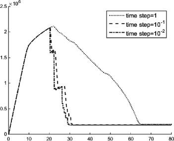
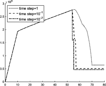
Figure 3: Evolution of averaged elastic von Mises stresses $\int_{\Omega}|\operatorname*{dev}\sigma_{\rm el}|\,\mathrm{d}x$ over time for the two experiments from Fig. 2 for three different time discretisations. The left experiment ruptures earlier under less stretch and leaving less plastification and remaining stress comparing to the right experiment. In both experiments, the convergence theoretically supported by Proposition 4.2 is well documented.

One can also note that Figure 3-right imitates quite well the scenario from Figure 1-right while Figure 3-left is rather a mixture of both regimes from Figure 1 and, interestingly, the rupture proceeds in three stages. The respective spacial distribution of the evolving state variable is depicted at few selected instants on Figures 4 and 5.

DAMAGE $\zeta$        PLASTIC STRAIN $|\pi|$      STRESS $|\operatorname*{dev}\sigma_{\mathrm{el}}|$        RESIDUUM ${\rm log}\,|R|$         
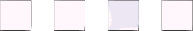
 ${}^{{}^{{}^{{}^{{}^{{}^{{}^{\text{\small$t=4\ \ $}}}}}}}}$
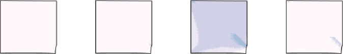
 ${}^{{}^{{}^{{}^{{}^{{}^{{}^{\text{\small$t=8\ \ $}}}}}}}}$
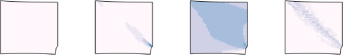
 ${}^{{}^{{}^{{}^{{}^{{}^{{}^{\text{\small$t=12$}}}}}}}}$
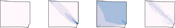
 ${}^{{}^{{}^{{}^{{}^{{}^{{}^{\text{\small$t=16$}}}}}}}}$
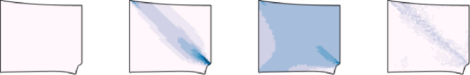
 ${}^{{}^{{}^{{}^{{}^{{}^{{}^{\text{\small$t=20$}}}}}}}}$
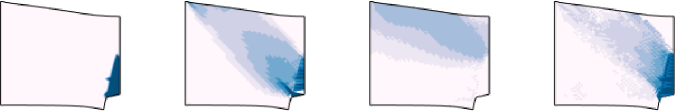
 ${}^{{}^{{}^{{}^{{}^{{}^{{}^{\text{\small$t=24$}}}}}}}}$
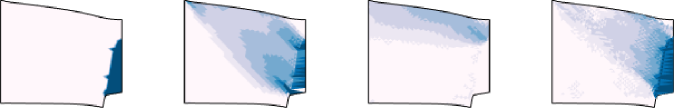
 ${}^{{}^{{}^{{}^{{}^{{}^{{}^{\text{\small$t=28$}}}}}}}}$
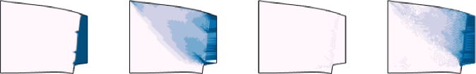
 ${}^{{}^{{}^{{}^{{}^{{}^{{}^{\text{\small$t=32$}}}}}}}}$
   

Figure 4: Evolution of spatial distribution of the state $(u,\pi,\zeta)$ with also the von Mises stress and the residuum $R$ from (4.23) at (equidistantly) selected instants for the asymmetric geometry from Fig. 2-left. The deformation is visualized by a displacement $u$ magnified 250$\,\times$, and $\tau=0.1$ was used. Damage occurs relatively early on the right-hand side due to the stress concentration and propagates in several partial steps, cf. Fig. 3-left.

DAMAGE $\zeta$        PLASTIC STRAIN $|\pi|$      STRESS $|\operatorname*{dev}\sigma_{\mathrm{el}}|$        RESIDUUM ${\rm log}\,|R|$         
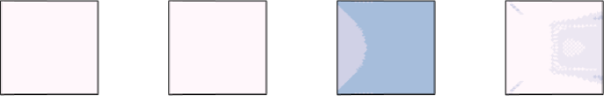
 ${}^{{}^{{}^{{}^{{}^{{}^{{}^{\text{\small$t=10$}}}}}}}}$
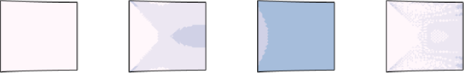
 ${}^{{}^{{}^{{}^{{}^{{}^{{}^{\text{\small$t=20$}}}}}}}}$
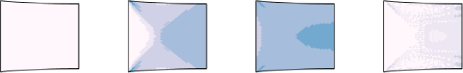
 ${}^{{}^{{}^{{}^{{}^{{}^{{}^{\text{\small$t=30$}}}}}}}}$
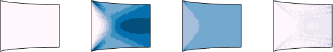
 ${}^{{}^{{}^{{}^{{}^{{}^{{}^{\text{\small$t=50$}}}}}}}}$
 ${}^{{}^{{}^{{}^{{}^{{}^{{}^{\text{\small$t=54$}}}}}}}}$
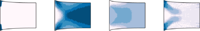
 ${}^{{}^{{}^{{}^{{}^{{}^{{}^{\text{\small$t=55$}}}}}}}}$
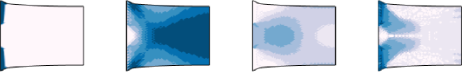
 ${}^{{}^{{}^{{}^{{}^{{}^{{}^{\text{\small$t=56$}}}}}}}}$
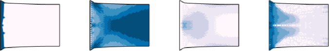
 ${}^{{}^{{}^{{}^{{}^{{}^{{}^{\text{\small$t=57$}}}}}}}}$
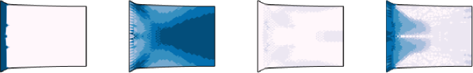
 ${}^{{}^{{}^{{}^{{}^{{}^{{}^{\text{\small$t=60$}}}}}}}}$
   

Figure 5: Evolution of spatial distribution of the state $(u,\pi,\zeta)$ with also the von Mises stress and the residuum $R$ from (4.23) at selected instants for the symmetric geometry from Fig. 2-right. The deformation is visualized by a displacement $u$ magnified 250$\,\times$, and $\tau=0.1$ was used. The process inherits the symmetry of the specimen and loading. In contrast to Fig. 4, damage occurs rather later on the left-bottom corner and propagates fast, hence the snapshots are selected not in an equidistant way here.

It is well seen how a relatively small variation of geometry in Figure 2 dramatically changes the spatial scenario and triggers damage in very different spots of the specimen. This is an expected notch-effect causing stress concentration and relatively early initiation of cracks at such spots, i.e. here such a notch is the point of the transition $\Gamma_{\mbox{\tiny\rm N}}$ to $\mathchoice{\Gamma_{\mbox{\tiny\rm D}}}{\Gamma_{\mbox{\tiny\rm D}}}{\Gamma_{\mbox{\tiny\rm D}}}{\Gamma_{\mbox{\tiny\rm D}}}/\Gamma_{\mbox{\tiny\rm N}}$ in Figure 2-left. The AMDP suggested in Remark 4.3 is depicted in Figures 6 and 7. It should be emphasized that the maximum-dissipation principle (as devised originally by Hill [16]) is reliably satisfied only for convex stored energies as occurs during mere plastification phase, as also seen in Figure 7, while in general it does not need to be satisfied even in obviously physically relevant stress-driven evolutions, as already mentioned in Remark 3.3 and which can be expected even here during massive fast rupture of a wider regions (but in spite of it, Figure 6 shows a good satisfaction of AMDP even during such rupture phases and in some sense demonstrate a good applicability of the model and solution concept and its algorithmic realization).

Remark 6.1 (Symmetry issue).

Actually, one could understood the square 1$\,\times\,1$ in Fig. 2 as one half of a rectangle with sides 2$\,\times\,1$ with the right-hand side of the 1$\,\times\,1$ square being the symmetry axis of the 2$\,\times\,1$ rectangle which is then loaded from the vertical sides fully symmetrically. Engineers actually most routinely assume that such symmetry of this geometry would be inheritted by all (or at least by one) solution(s) and use the reduced geometries on Fig. 2 for calculations of the full 2$\,\times\,1$-rectangle. We intentionally did not use this interpretation because, in fact, one can only say that the set of all solutions inherits the (possible) symmetry of the specimen and its loading but not particular solutions, and even it may be that there is no solution inheritting this symmetry or that experimental evidence shows preferences for nonsymmetric solutions. Cf. the discussion in [12, 26]. In addition, the geometry in Fig. 2-left would lead to a 2$\,\times\,1$ rectangle with a partial “cut” in the mid-bottom side, which is not a Lipschitz domain.

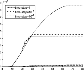
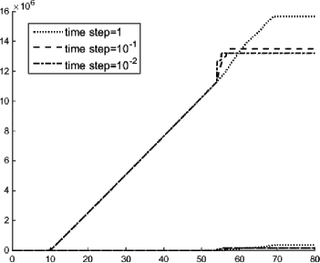
Figure 6: Evolution of the dissipated energy $\mathrm{Diss}_{\mathscr{R}}(z;[0,t])$ (top 3 curves) and integrated residua $\int_{0}^{t}\int_{\Omega}R\,\mathrm{d}x\mathrm{d}t$ (bottom 3 curves) in two experiments from Figure 2. In particular, it again shows good tendency of convergence and, moreover, that the violation of the approximate maximum-dissipation principle is small with respect to the overall dissipated energy and the evolution was stress driven with a good accuracy about 1-2%.

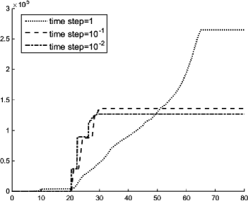
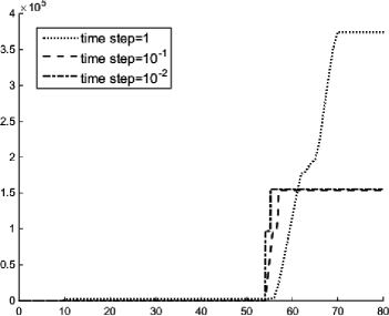
Figure 7: A detailed scaling of the bottom 3 curves (= the residua in AMDP) from Figure 6. A good convergence to zero is seen in plastification period while some residuum is generated during damage period where nonconvexity of the stored energy truly comes into effect.

Remark 6.2 (Recovery of the integrated maximum-dissipation principle IMDP).

It should be emphasized that, even if the intuitively straightforward AMDP is asymptotically satisfied, the recovery of even the less-selective IMDP (3.8) for $\tau\to 0$ is not clear. This is obviously related with instability of IMDP under data perturbation if $\mathscr{E}(t,\cdot)$ is not convex. Here, to recover the IMDP on $I$, it would suffice to show that for all $\varepsilon>0$ there is $\tau_{\varepsilon}>0$ such that for any $0<\tau\leq\tau_{\varepsilon}$ it holds

$$\sum_{k=1}^{T/\tau}\inf_{t\in[k\tau-\tau,k\tau]}\big{\langle}\xi(t),z(k\tau){-}z(k\tau{-}\tau)\big{\rangle}-\mathscr{R}\big{(}z(k\tau){-}z(k\tau{-}\tau)\big{)}\geq-\varepsilon$$ (6.1)

for some selection $\xi(t)\in-\partial_{z}\mathscr{E}(t,u(t),z(t))$, cf. the definition (3.7) and realize that the equi-distant partitions are cofinal in all partitions of $I$. This can be guaranteed only under rather strong conditions, namely if, for all $\varepsilon>0$, there is $\tau_{\varepsilon}>0$ such that for any $0<\tau\leq\tau_{\varepsilon}$, the following strengthened version of the AMDP

$$\sum_{k=1}^{T/\tau_{\varepsilon}}\mathscr{R}\big{(}\mathchoice{\text{\large$\hskip 0.35999pt\overline{\text{\normalsize$z$}}\hskip 0.35999pt$}}{\text{\large$\hskip 0.35999pt\overline{\text{\normalsize$z$}}\hskip 0.35999pt$}}{\text{\normalsize$\overline{\text{\normalsize$z$}}$}}{\text{\small$\bar{\text{\tiny$z$}}$}}_{\tau}(t_{k})-\mathchoice{\text{\large$\hskip 0.35999pt\overline{\text{\normalsize$z$}}\hskip 0.35999pt$}}{\text{\large$\hskip 0.35999pt\overline{\text{\normalsize$z$}}\hskip 0.35999pt$}}{\text{\normalsize$\overline{\text{\normalsize$z$}}$}}{\text{\small$\bar{\text{\tiny$z$}}$}}_{\tau}(t_{k-1})\big{)}-\big{\langle}\mathchoice{\text{\large$\hskip 0.35999pt\overline{\text{\normalsize$\xi$}}\hskip 0.35999pt$}}{\text{\large$\hskip 0.35999pt\overline{\text{\normalsize$\xi$}}\hskip 0.35999pt$}}{\text{\normalsize$\overline{\text{\normalsize$\xi$}}$}}{\text{\small$\bar{\text{\tiny$\xi$}}$}}_{\tau}(t),\mathchoice{\text{\large$\hskip 0.35999pt\overline{\text{\normalsize$z$}}\hskip 0.35999pt$}}{\text{\large$\hskip 0.35999pt\overline{\text{\normalsize$z$}}\hskip 0.35999pt$}}{\text{\normalsize$\overline{\text{\normalsize$z$}}$}}{\text{\small$\bar{\text{\tiny$z$}}$}}_{\tau}(t_{k})-\mathchoice{\text{\large$\hskip 0.35999pt\overline{\text{\normalsize$z$}}\hskip 0.35999pt$}}{\text{\large$\hskip 0.35999pt\overline{\text{\normalsize$z$}}\hskip 0.35999pt$}}{\text{\normalsize$\overline{\text{\normalsize$z$}}$}}{\text{\small$\bar{\text{\tiny$z$}}$}}_{\tau}(t_{k-1})\big{\rangle}\leq\varepsilon$$ (6.2)

holds for $t_{k}=k\tau_{\varepsilon}$, any $t_{k-1}\leq t\leq t_{k}$, and some $\mathchoice{\text{\large$\hskip 0.35999pt\overline{\text{\normalsize$\xi$}}\hskip 0.35999pt$}}{\text{\large$\hskip 0.35999pt\overline{\text{\normalsize$\xi$}}\hskip 0.35999pt$}}{\text{\normalsize$\overline{\text{\normalsize$\xi$}}$}}{\text{\small$\bar{\text{\tiny$\xi$}}$}}_{\tau}(t)\!\in\!-\partial_{z}\mathscr{E}(t,\mathchoice{\text{\large$\hskip 0.35999pt\overline{\text{\normalsize$u$}}\hskip 0.35999pt$}}{\text{\large$\hskip 0.35999pt\overline{\text{\normalsize$u$}}\hskip 0.35999pt$}}{\text{\normalsize$\overline{\text{\normalsize$u$}}$}}{\text{\small$\bar{\text{\tiny$u$}}$}}_{\tau}(t),\mathchoice{\text{\large$\hskip 0.35999pt\overline{\text{\normalsize$z$}}\hskip 0.35999pt$}}{\text{\large$\hskip 0.35999pt\overline{\text{\normalsize$z$}}\hskip 0.35999pt$}}{\text{\normalsize$\overline{\text{\normalsize$z$}}$}}{\text{\small$\bar{\text{\tiny$z$}}$}}_{\tau}(t))$, and if $\mathchoice{\text{\large$\hskip 0.35999pt\overline{\text{\normalsize$\xi$}}\hskip 0.35999pt$}}{\text{\large$\hskip 0.35999pt\overline{\text{\normalsize$\xi$}}\hskip 0.35999pt$}}{\text{\normalsize$\overline{\text{\normalsize$\xi$}}$}}{\text{\small$\bar{\text{\tiny$\xi$}}$}}_{\tau}(t)\rightharpoonup\xi(t)$, which can be assumed due to the available a-priori estimates used in the proof of Proposition 4.2. Using also (4.13) and the (norm,weak)-upper semicontinuity of $\partial_{z}\mathscr{E}(t,\cdot,\cdot)$, in the limit for $\tau\to 0$, from such a strengthened AMDP, one can read $\sum_{k=1}^{T/\tau_{\varepsilon}}\mathscr{R}(z(t_{k})-z(t_{k-1}))-\langle\xi(t),z(t_{k})-z(t_{k-1})\rangle\leq\varepsilon$ for any $t_{k-1}\leq t\leq t_{k}$ and for some $\xi(t)\in-\partial_{z}\mathscr{E}(t,u(t),z(t))$, from which (6.1) indeed follows. In fact, our intuitive version of AMDP from Remark 4.3 computationally verified (6.2) in Figure 7 in particular examples for $\tau=\tau_{\varepsilon}$ only. And, on top of it, we would need (6.2) to be shown rather for $\bar{\xi}_{\tau}\in(-\partial_{\pi}\mathscr{E}(t,\mathchoice{\text{\large$\hskip 0.35999pt\overline{\text{\normalsize$u$}}\hskip 0.35999pt$}}{\text{\large$\hskip 0.35999pt\overline{\text{\normalsize$u$}}\hskip 0.35999pt$}}{\text{\normalsize$\overline{\text{\normalsize$u$}}$}}{\text{\small$\bar{\text{\tiny$u$}}$}}_{\tau}(t),\mathchoice{\text{\large$\hskip 0.35999pt\overline{\text{\normalsize$z$}}\hskip 0.35999pt$}}{\text{\large$\hskip 0.35999pt\overline{\text{\normalsize$z$}}\hskip 0.35999pt$}}{\text{\normalsize$\overline{\text{\normalsize$z$}}$}}{\text{\small$\bar{\text{\tiny$z$}}$}}_{\tau}(t{-}\tau)),-\partial_{\zeta}\mathscr{E}(t,\mathchoice{\text{\large$\hskip 0.35999pt\overline{\text{\normalsize$u$}}\hskip 0.35999pt$}}{\text{\large$\hskip 0.35999pt\overline{\text{\normalsize$u$}}\hskip 0.35999pt$}}{\text{\normalsize$\overline{\text{\normalsize$u$}}$}}{\text{\small$\bar{\text{\tiny$u$}}$}}_{\tau}(t),\mathchoice{\text{\large$\hskip 0.35999pt\overline{\text{\normalsize$z$}}\hskip 0.35999pt$}}{\text{\large$\hskip 0.35999pt\overline{\text{\normalsize$z$}}\hskip 0.35999pt$}}{\text{\normalsize$\overline{\text{\normalsize$z$}}$}}{\text{\small$\bar{\text{\tiny$z$}}$}}_{\tau}(t)))$.

Acknowledgments. This research has been supported by GA ČR through the projects 13-18652S “Computational modeling of damage and transport processes in quasi-brittle materials” and 14-15264S “Experimentally justified multiscale modelling of shape memory alloys” with also the also institutional support RVO:61388998 (ČR).

References

- [1] J. Alberty, C. Carstensen, and D. Zarrabi. Adaptive numerical analysis in primal elastoplasticity with hardening. Comput. Methods Appl. Mech., 171:175–204, 1999.
- [2] R. Alessi, J.-J. Marigo, and S. Vidoli. Gradient damage models coupled with plasticity and nucleation of cohesive cracks. Arch. Rational Mech. Anal, 214:575–615, 2014.
- [3] R. Alessi, J.-J. Marigo, and S. Vidoli. Gradient damage models coupled with plasticity: Variational formulation and main properties. Mech. of Materials, 80 B:351–367, 2015.
- [4] M. A. Biot. Mechanics of Incremental Deformations. J. Wiley, New York, 1965.
- [5] E. Bonetti, M. Frémond, and C. Lexcellent. Global existence and uniqueness for a thermomechanical model for shape memory alloys with partition of the strain. Math. Mech. Solids, 11:251–275, 2006.
- [6] M. Brokate, C. Carstensen, and J. Valdman. A quasi-static boundary value problem in multi-surface elastoplasticity. II: Numerical solution. Math. Methods Appl. Sci., 28:881–901, 2005.
- [7] M. Čermák, T. Kozubek, S. Sysala, and J. Valdman. A TFETI domain decomposition solver for elastoplastic problems. Appl. Math. Comput., 231:634–653, 2014.
- [8] L. Contrafatto and M. Cuomo. A new thermodynamically consistent continuum model for hardening plasticity coupled with damage. Intl. J. Solids Structures, submitted.
- [9] V. Crismale. Globally stable quasistatic evolution for a coupled elastoplastic-damage problem. Preprint SISSA 34/2014/MATE, 2014.
- [10] M. Frémond. Non-Smooth Thermomechanics. Springer-Verlag, Berlin, 2002.
- [11] M. Frost, B. Benešová, and P. Sedlák. A microscopically motivated constitutive model for shape memory alloys: formulation, analysis and computations. Math. Mech. of Solids, 2014. DOI:10.1177/1081286514522474.
- [12] I. G. García, V. Mantič, and E. Graciani. Debonding at the fibre-matrix interface under remote transverse tension. one debond or two symmetric debonds? Europ. J. of Mechanics A/Solids, 53:75–88, 2015.
- [13] P. Gruber, D. Knees, S. Nesenenko, and M. Thomas. Analytical and numerical aspects of time-dependent models with internal variables. Zeitschrift f. angew. Math. und Mechanik, 90:861–902, 2010.
- [14] P. Gruber and J. Valdman. Solution of one-time-step problems in elastoplasticity by a Slant Newton Method. SIAM J. Scientific Computing, 31:1558–1580, 2009.
- [15] W. Han and B. D. Reddy. Plasticity (Mathematical Theory and Numerical Analysis). Springer-Verlag, New York, 1999.
- [16] R. Hill. A variational principle of maximum plastic work in classical plasticity. Q.J. Mech. Appl. Math., 1:18–28, 1948.
- [17] D. Knees, R. Rossi, and C. Zanini. A vanishing viscosity approach to a rate-independent damage model. Math. Models Meth. Appl. Sci., 23:565–616, 2013.
- [18] P. Krejčí and U. Stefanelli. Existence and non-existence for the full thermomechanical Souza-Auricchio model of shape memory wires. Math. Mech. Solids, 16:349–365, 2011.
- [19] D. Leguillon. Strength or toughness? A criterion for crack onset at a notch. European J. of Mechanics A/Solids, 21:61–72, 2002.
- [20] A. Mielke. Differential, energetic, and metric formulations for rate-independent processes. In L. Ambrosio and G. Savaré, editors, Nonlinear PDE’s and Applications, pages 87–170. Springer, 2011. (C.I.M.E. Summer School, Cetraro, Italy 2008, Lect. Notes Math. Vol. 2028).
- [21] A. Mielke and T. Roubíček. Rate Independent Systems - Theory and Application. Springer, New York, 2015.
- [22] A. Mielke and F. Theil. On rate-independent hysteresis models. Nonl. Diff. Eqns. Appl., 11:151–189, 2004.
- [23] E. H. Moore. Definition of limit in general integral analysis. Proc. Nat. Acad. Sci. U.S.A., 1:628–632, 1915.
- [24] Q.-S. Nguyen. Some remarks on standard gradient models and gradient plasticity. Math. Mech. of Solids, 2014, printed on line. DOI:10.1177/1081286514551499.
- [25] C. G. Panagiotopoulos, V. Mantič, and T. Roubíček. Two adhesive-contact models for quasistatic mixed-mode delamination problems. Math. Comput. in Simulation, 2014. Submitted.
- [26] C. G. Panagiotopoulos and V. Mantič. Symmetric and non–symmetric debonds at fiber-matrix interface under transverse loads. an application of energetic approaches using collocation BEM. Anales de Mecánica de la Fractura, 30:125–130, 2013.
- [27] S. Pollard. The Stieltjes’ integral and its generalizations. Quart. J. of Pure and Appl. Math., 49:73–138, 1923.
- [28] T. Rahman and J. Valdman. Fast MATLAB assembly of FEM matrices in 2D and 3D: nodal elements. Appl. Math. Comput, 219:7151–7158, 2013.
- [29] T. Roubíček. Rate independent processes in viscous solids at small strains. Math. Methods Appl. Sci., 32:825–862, 2009. Erratum Vol. 32(16) p. 2176.
- [30] T. Roubíček. Nonlinear Partial Differential Equations with Applications. Birkhäuser, Basel, 2nd edition, 2013.
- [31] T. Roubíček. Maximally-dissipative local solutions to rate-independent systems and application to damage and delamination problems. Nonlin. Anal, Th. Meth. Appl., 113:33–50, 2015.
- [32] T. Roubíček, M. Kružík, and J. Zeman. Delamination and adhesive contact models and their mathematical analysis and numerical treatment. In V. Mantič, editor, Math. Methods & Models in Composites, chapter 9, pages 349–400. Imperial College Press, 2013.
- [33] T. Roubíček, V. Mantič, and C. G. Panagiotopoulos. Quasistatic mixed-mode delamination model. Discr. Cont. Dynam. Systems Ser. S, 6:591–610, 2013.
- [34] T. Roubíček, C. G. Panagiotopoulos, and V. Mantič. Quasistatic adhesive contact of visco-elastic bodies and its numerical treatment for very small viscosity. Zeitschrift angew. Math. Mech., 93:823–840, 2013.
- [35] T. Roubíček, C. G. Panagiotopoulos, and V. Mantič. Local-solution approach to quasistatic rate-independent mixed-mode delamination. Math. Models Meth. Appl. Sci., 25:1337–1364, 2015.
- [36] T. Roubíček and J. Valdman. Perfect plasticity with damage and healing at small strains, its modelling, analysis, and computer implementation (Preprint arXiv no.1505.01018). SIAM J. Appl. Math., submitted.
- [37] A. Sadjadpour and K. Bhattacharya. A micromechanics inspired constitutive model for shape-memory alloys. Smart Mater. Structures, 16:1751–1765, 2007.
- [38] P. Sedlák, M. Frost, B. Benešová, T. Ben Zineb, and P. Šittner. Thermomechanical model for NiTi-based shape memory alloys including R-phase and material anisotropy under multi-axial loadings. Int. J. Plasticity, 39:132–151, 2012.
- [39] U. Stefanelli. A variational characterization of rate-independent evolution. Mathem. Nach., 282:1492–1512, 2009.
- [40] R. Toader and C. Zanini. An artificial viscosity approach to quasistatic crack growth. Boll. Unione Matem. Ital., 2:1–36, 2009.
- [41] J. Valdman. Continuum undergoing combined elasto-plasto-damage. Matlab package. http://www.mathworks.com/matlabcentral/fileexchange/authors/37756.
- [42] R. Vodička, V. Mantič, and T. Roubíček. Energetic versus maximally-dissipative local solutions of a quasi-static rate-independent mixed-mode delamination model. Meccanica, 49:2933–2963, 2014.
- [43] H. Ziegler. An attempt to generalize Onsager’s principle, and its significance for rheological problems. Zeitschrift angew. Math. Physik, 9:748–763, 1958.