Deep near-IR observations of the Globular Cluster M 4: Hunting for Brown Dwarfs.

Abstract

We present an analysis of deep HST/WFC3 near-IR (NIR) imaging data of the globular cluster M 4. The best-photometry NIR colour-magnitude diagram (CMD) clearly shows the main sequence extending towards the expected end of the Hydrogen-burning limit and going beyond this point towards fainter sources. The white dwarf sequence can be identified. As such, this is the deepest NIR CMD of a globular cluster to date. Archival HST optical data were used for proper-motion cleaning of the CMD and for distinguishing the white dwarfs (WDs) from brown dwarf (BD) candidates. Detection limits in the NIR are around $F110W\approx 26.5$ mag and $F160W\approx 27$ mag, and in the optical around $F775W\approx 28$ mag. Comparing our observed CMDs with theoretical models, we conclude that we have reached beyond the H-burning limit in our NIR CMD and are probably just above or around this limit in our optical-NIR CMDs. Thus, any faint NIR sources that have no optical counterpart are potential BD candidates, since the optical data are not deep enough to detect them. We visually inspected the positions of NIR sources which are fainter than the H-burning limit in $F110W$ and for which the optical photometry did not return a counterpart. We found in total five sources for which we did not get an optical measurement. For four of these five sources, a faint optical counterpart could be visually identified, and an upper optical magnitude was estimated. Based on these upper optical magnitude limits, we conclude that one source is likely a WD, one source could either be a WD or BD candidate, and the remaining two sources agree with being BD candidates. For only one source no optical counterpart could be detected, which makes this source a good BD candidate. We conclude that we found in total four good BD candidates.

1 Introduction

Globular clusters (GCs) are the oldest and most massive stellar aggregates in our Galaxy. As such, they are the best natural laboratories to study large, co-eval populations of stars at known distance and metallicity. Indeed, much of our understanding of star formation and evolution has been derived from observational studies of GCs. Nonetheless, we still lack an understanding of the very low mass stars (VLMSs) around the faint end of the Hydrogen-burning main sequence (MS) and of objects beyond that limit, i.e., sub-stellar sources, so called “Brown Dwarfs” (BDs). This is especially true for objects at the low-metallicities typical for the GCs in our Milky Way (see below).

BDs present a link between stars and planets, and thus are important for our understanding of both star and planet formation and evolution. BDs are sub-stellar objects that are not massive enough to ignite and sustain Hydrogen burning. Thus, where low-mass stars will retain their luminosity for a Hubble time or longer, a BD will continue to cool and become fainter with age. Like giant gas planets, BDs have complex atmospheres (Burrows et al., 1997, 2001). The distinction between stars, BDs and planets is either based on mass or on formation. In general, stars have masses $>80M_{J}$ and can sustain Hydrogen burning, BDs have masses between 80 and 13 $M_{J}$ and cannot sustain Hydrogen burning but a short period of Deuterium burning, and giant planets have masses below 13 $M_{J}$ and cannot sustain Deuterium burning (Burrows et al. 1997, Stamatellos 2014, but see also Sect. 3.3). Because low-mass stars and BDs have life-times much longer than the age of the Galaxy, the GC VLMSs and BDs are also important tracers of Galactic formation and chemical evolution.

The formation of BDs is a matter of considerable dispute. They might have formed in the same way as (low-mass) stars from turbulent cloud fragmentation (Elmegreen, 1999; Whitworth & Goodwin, 2005; André et al., 2012), which would imply a continuous extension of the IMF into the sub-stellar regime. On the other hand, BDs might form e.g. from the ejection of stellar embryos or sub-stellar clumps which did not have the chance to accumulate enough mass (Reipurth & Clarke, 2001; Basu & Vorobyov, 2012). Kroupa & Bouvier (2003) suggested that BDs form via photo-evaporation of protostars through nearby massive stars. This might also suggest an increase in the number of BDs with cluster mass, as more massive clusters have more O stars which can produce more BDs. BDs might also form from the fragmentation of circumstellar disks (Stamatellos et al. 2011, Thies et al. 2010, Kaplan et al. 2012). In this case, the number of BDs in clusters could be enhanced in dense clusters as dynamical interactions between cluster stars lead to more disk fragmentation. Thies et al. (2015) concluded that BDs likely form not just via one formation scenario, but from a combination of various channels.

Large surveys undertaken in the past decade have detected large numbers of BDs. For example, the Two Micron All Sky Survey (2MASS; Skrutskie et al. 2006), the Sloan Digital Sky Survey (SDSS; York et al. 2000), the United Kingdom Infrared telescope Deep Sky Survey (UKIDSS; Lawrence et al. 2007), the Wide-field Infrared Survey Explorer (WISE, Wright et al. 2010) all sky survey have been very successful in finding such cool, low-mass objects. However, for most of these BDs, key physical properties like metallicity and age are unconstrained (see e.g. DwarfArchives.org). In fact, determining the physical parameters is extremely difficult and a major hurdle in BD research. Observations of open star clusters and star forming regions, where all sources are at the same distance and metallicity, can mitigate this problem (e.g. Steele et al. 1995, Rebolo et al. 1996, Martín et al. 2001, Pinfield et al. 2003, Boudreault & Lodieu 2013, Casewell et al. 2014), but only for young and metal-rich objects. Thus the need for benchmark sources is especially evident for the metal-poor regime, and indeed we still do not know much about old, metal-poor BDs. So far, only very few low-metallicity, old VLMSs near the H-burning limit, and even fewer sub-stellar (candidate) halo objects have been identified (e.g. Burgasser et al. 2003, 2009, Lépine et al. 2004, Burgasser & Kirkpatrick 2006, Cushing et al. 2009, Sivarani et al. 2009, Murray et al. 2011, Mace et al. 2013, Pinfield et al. 2014, Luhman & Sheppard 2014, Burningham et al. 2014, Kirkpatrick et al. 2014).

This is where GCs come in: they are massive, and thus might have produced BDs in large numbers, and they are also the oldest and most metal-poor stellar aggregates in our Galaxy. Potentially, GCs are the ideal hunting ground for old, metal-poor benchmark VLMSs and BDs which are much needed if we are to test stellar and sub-stellar formation and evolution theories and models of metal-poor (sub-)stellar atmospheres.

However, identifying substellar objects in GC is challenging due to their intrinsic faintness. Therefore, the closest GCs make the best targets for this kind of research. Out of the GCs in our Galaxy, M 4 (NGC 6121) is the closest GC to us; distance estimates range from 1.7 kpc (Hansen et al. 2004) to $\approx$ 2 kpc (e.g. Bedin et al. 2009). Braga et al. (2015) estimated a true distance modulus of 11.28 mag based on RR Lyrae period-luminosity and period-Wesenheit relations, resulting in a distance of 1.8 kpc, which agrees well with previous estimates. Malavolta et al. (2014) analyzed 7250 spectra for 2771 cluster stars and found a metallicity of $\rm[Fe/H]=-1.07$ dex (RGB) to $\rm[Fe/H]=-1.16$ dex (sub giant branch and MS stars), which is well in line with previous metallicity estimates (e.g. $\rm[Fe/H]=-1.15$ dex according to the 2010 update of the Harris, 1996, catalogue of globular clusters in the Milky Way).

As such, M 4 is a prime target for ultra-deep observational studies. Indeed, deep optical studies with the Hubble Space Telescope (HST) have been undertaken by Richer et al. (1997, 2004) and Bedin et al. (2009), yielding impressive results. Richer et al. (1997, 2004) estimated the fraction of similar-mass photometric binaries to be small (just 2% in their outer field, falling to just 1% towards the cluster core). Milone et al. (2012) suggested a much higher total binary fraction, raising from 10% at the halfmass radius to 15% towards the cluster core. The present day mass function of the lower-mass MS stars is flat (Bedin et al. 2001), with a slope of $\alpha=0.1$ and a further flattening towards the cluster centre (Richer et al. 2004). The cluster WDs suggest that the initial mass function (IMF) above 0.8 $M_{\odot}$ was much steeper than the present day mass function. Bedin et al. (2009) presented the deepest optical colour-magnitude diagram (CMD) to date of this cluster and located the faint end of the WD cooling sequence in M 4 at $F606W=28.5$ mag, suggesting an age of 11.6$\pm$0.6 Gyr. This agrees with the finding of Hansen et al. (2004), who found a WD based age of 12.1 Gyr. The ongoing HST M 4 core project (PI L. Bedin, GO-12911) searches for binary dark companions to MS stars. The high-accuracy astrometry and photometry of this data-set, together with archival material and a part of the deep near-IR (NIR) data presented in this paper, have already been used to identify two distinct sequences along the lower-mass MS (Milone et al., 2014).

M 4 is also so far the only GC known to host a planetary system, PSR B1620-26 (Sigurdsson et al. 2003), which challenged the planet-metallicity relation of the standard planet formation model at that time (Fischer & Valenti, 2005). Recently, Hasegawa & Hirashita (2014) suggested that the critical metallicity for gas giant formation is [Fe/H]$\approx−1.2$ dex, which agrees with M 4’s metallicity. Beer et al. (2004) suggested a metallicity-independent formation scenario, in which the planet in M 4 formed through dynamically induced instability in a circumbinary disc. If true, then we can expect many planets to form especially in the dense GCs in which dynamical interactions between cluster stars are ubiquitous. Since BDs might form in a similar way, we then might also expect that many more BDs form in dense GCs compared to open clusters.

This paper is structured as follows. In Section 2 we describe the observations and reduction of our NIR and archival optical data. In Section 3 we present and discuss the NIR and optical-NIR CMDs, and our results and conclusions are summarized in Section 4.

2 Observations

2.1 NIR Data

The NIR observations of the globular cluster M 4 were carried out in April 2012 with the Wide Field Camera 3 (WFC3) on board the HST, using the $F110W$ and $F160W$ filters (program GO–12602, PI: Dieball). All observations were made at a single pointing position on a field centred at about one core radius North East from the cluster centre. This region in the cluster had been the focus of the programs GO-5461 (Richer et al. 1997, 2004) and GO–10146 (Bedin et al. 2009) and thus is fully covered by deep optical observations. A standard 4-point WFC3-IRDITHER-BOX-MIN dither pattern and a sampling of NSAMP14 SPARS50 was applied during the observations to get a well-sampled point spread function (PSF). The WFC3 field of view is $136\arcsec\times 123\arcsec$ in the IR channel, with a resolution of $0.13\arcsec\times 0.121\arcsec$ per pixel. All NIR observations were carried out during two consecutive orbits on April 16th ($F110W$) and four orbits on April 20th to 21st ($F160W$), comprising a total of 8 individual images in $F110W$ and 16 images in $F160W$, each 653 seconds, resulting in total exposure times of 5223 seconds ($F110W$) and 10447 seconds ($F160W$).

Using the pipeline produced flat-fielded (FLT) images, we first created a master image for each of our IR filters, using multidrizzle running under PyRAF (the Python-based interface to IRAF). multidrizzle corrects geometric distortions that are present in the input images and combines them into a master image. Shifts between the individual images are expected, as we have applied a dither pattern. On top of this, telescope breathing can affect guide star tracking and as a result can cause small shifts, typically on a sub-pixel scale (see e.g. the multidrizzle handbook available on the STScI webpages). In order to ascertain that all shifts are taken into account, we created geometric-distortion corrected individual images. Based on the coordinates of the same 10 stars in each of these images (selected to be well distributed over the field of view), accurate shifts between the individual and the master images were then determined using tweakshift.

The master images created in this way are displayed in Figures 1 and 2. Note that these master images serve as reference images for the positions of the stars detected by DOLPHOT, but the photometry was actually performed on the individual images (see 2.2 below).

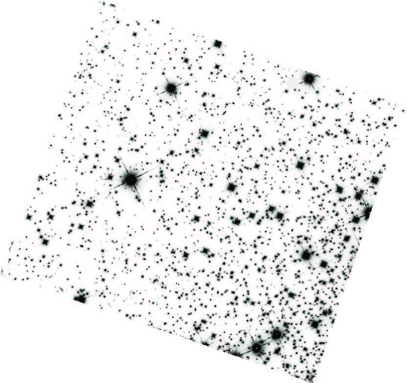
Figure 1: Left: Geometric-distortion corrected $F110W$ master image. North is up and East to the left. The field of view is $136\arcsec\times 123\arcsec$. The image is displayed on a logarithmic scale to bring out fainter sources.

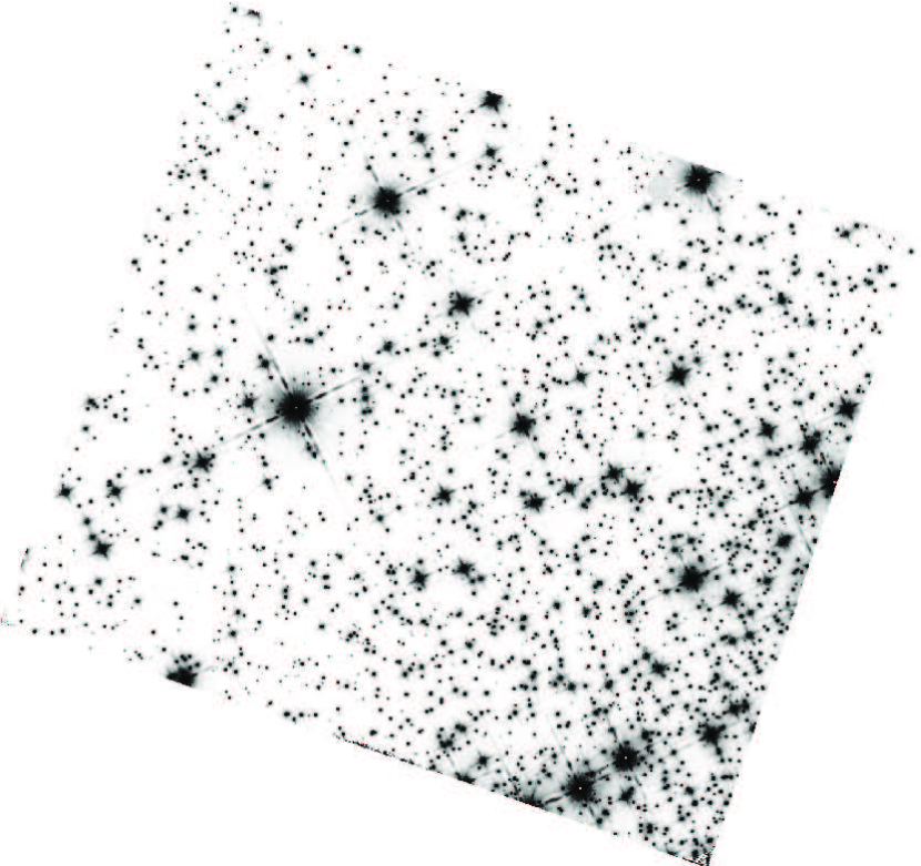
Figure 2: Same as Fig. 1 but for the $F160W$ data.

2.2 Photometry of the NIR data

Photometry was performed on the individual FLT images using the DOLPHOT software developed by A. Dolphin as a generalized version of HSTphot (Dolphin, 2000). DOLPHOT runs on the FLT images downloaded from the STScI archive, i.e., no further processing of the images is necessary nor recommended. Photometry is performed on each of the input images, using the WFC3 module which replaces the analytic PSF model with a look-up table computed using Tiny Tim PSFs (Krist & Hook 2011). For our data, we used Jay Anderson’s PSF libraries for the WFC3/IR filters and the pixel area maps available from the DOLPHOT webpage. The WFC3 module also includes a photometric calibration to the VEGAmag system. As a reference frame for a common physical (image) coordinate system we use our deepest image, i.e., the master image created with multidrizzle. The DOLPHOT package also provides routines to mask all pixels that are flagged as bad in the data quality arrays, to multiply with the pixel area maps, to calculate sky images, and to align all input images (or rather the source coordinates found in each input image) to the reference frame (our drizzled master images) using user defined lists of stellar coordinates in each input and the reference image. For these steps, we used the recommended WFC3 IR parameter settings.

Note that performing photometry on the drizzled image is expected to provide sub-optimal photometry, because the drizzling process affects the PSF and the noise characteristics of the drizzled images. Instead, DOLPHOT runs on all input images simultaneously and thus is capable of providing deep photometry. We started with the recommended parameters, and then refined some parameters to push our photometry as deep as possible.

DOLPHOT can run on data from multiple filters and cameras, thus we were able to do the photometry on both $F110W$ and $F160W$ data sets simultaneously. The output file includes x and y positions, photometric parameters like sharpness, crowding (the magnitude difference to the measured magnitude if no neighbouring sources would be fit simultaneously), the object type, and magnitudes in the VEGAmag system for all sources detected in the $F110W$ and $F160W$ data. A calibrated NIR CMD is plotted in Fig. 3. As can be seen, the CMD is exceptionally deep. The total catalogue contained 51 311 sources, but a large number of those will be spurious detections.

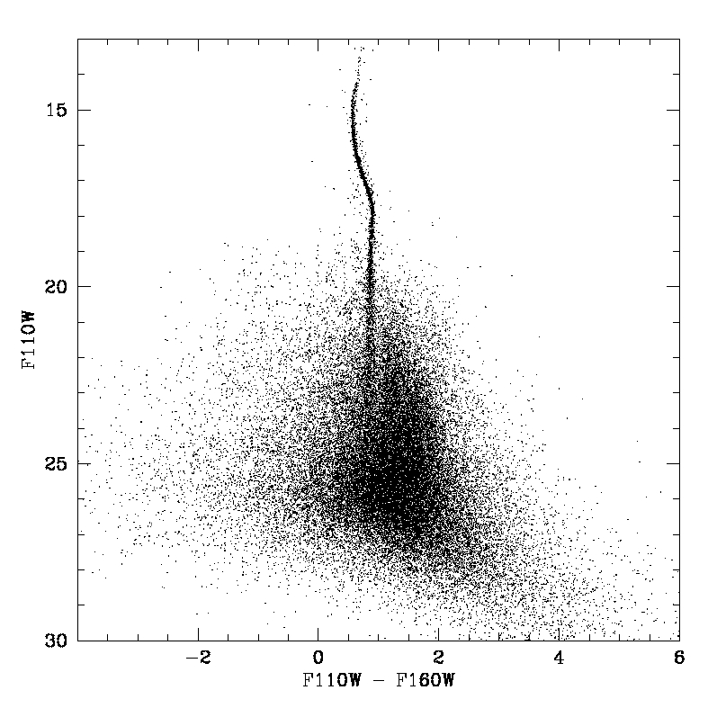
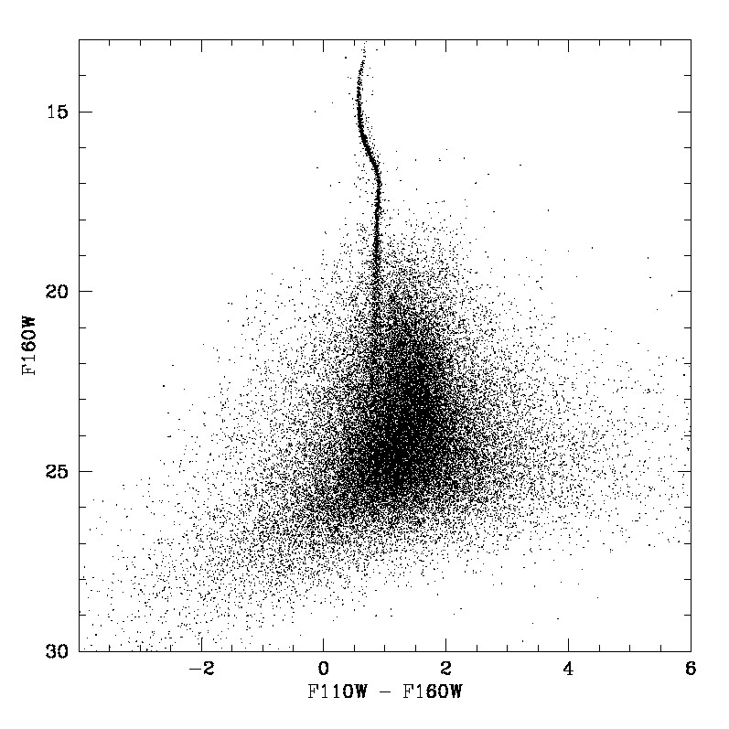
Figure 3: NIR CMDs of all sources detected by DOLPHOT. Left: $F110W$ vs. $F110W-F160W$, right: $F160W$ vs. $F110W-F160W$. Note that the CMDs are not selected and thus contain a large number of spurious detections like noise peaks and spikes around bright stars, but also faint sources that are not stars, and field stars that do not belong to the cluster.

2.3 Optical Data and photometry

Among the archival HST material the only images which offer any hope of detecting BDs in the optical are those deep and in the reddest filters available, i.e., $F775W$ and $F814W$ (indeed, technically $>$2/3 of these pass-bands are already in the NIR wavelength range).

We extensively searched in the HST archive, and identified four $\sim$1200 seconds deep images taken with ACS/WFC in $F775W$ under program GO-10146 (PI: Bedin) as the optimal for our purposes, as those images were taken in low-sky mode, are well dithered, and collected in a well defined epoch in 2005.48 (i.e., about 6.8 years before the GO-12602 data).

Images were reduced with the software described in great detail in Anderson et al. (2008). Briefly, the method is essentially a PSF-fitting where all pixels from all images are simultaneously fitted using the appropriate PSFs which account for the spatial and temporal shape-variation on each individual image. The key to the method is an optimal knowledge on how to transform those pixels into a common reference frame and an exquisite empirical PSF modeling. This software is well tested and used in all the twelve works of the series “The ACS Survey of Galactic Globular Clusters” (see, Sarajedini et al. 2007).

The first photometric run returned 19990 optical detections. As the detection of BDs might be only marginal in these optical images, we relaxed the finding criteria in a second photometric run, imposing to save all the local maxima, and not only the significant ones, resulting in 1.5 million detections. Although most of these local maxima likely are just fluctuations of the background noise, we can still use them to set an optical upper limit to the NIR-detected BD candidates.

For visual inspection of the WDs and BD candidates, stacked images were created from the CTE-corrected FLT images. The stacked images have pixels values resulting from median clipping of the CTE-corrected FLT individual images, and are supersampled by a factor of 2 in each direction (see Anderson et al. 2008 and Anderson & Bedin 2010 for further details).

3 The Colour-Magnitude Diagrams

We used the data in the two NIR filters $F110W$ and $F160W$ to create a NIR CMD. As the full NIR catalogue contains a large number of spurious detections, we created a best-photometry NIR CMD (described below in Sect. 3.1). However, since WDs and BD candidates have similar magnitudes and colours in the NIR, BD candidates cannot be distinguished based on the NIR data alone. We then used additional optical F775W data to create proper motion cleaned optical-NIR CMDs (see Sect. 3.1) in which the WD and MS sequence are clearly separate. Thus, the optical data are used to distinguish the WDs from the BD candidates.

3.1 Best-photometry NIR CMDs

In order to produce a clean CMD of only “good” stellar sources, we selected the output catalogue in such a way that the faint sources will be dominated by true stellar detections while keeping the number of spurious detections at bay. The resulting best-photometry catalogue includes 2526 sources, i.e, $\approx 5\%$ of all detections. The best-photometry CMD is remarkably clean, as can be seen in Fig. 4. We can clearly see the MS delineating down towards the expected H-burning limit and going beyond that to fainter sources. Note that this CMD is not proper motion cleaned, as we show all NIR sources that satisfy our selection criterion on the photometry. All sources with magnitudes fainter than 24 mag in $F110W$ were visually inspected on the $F110W$ master image, resulting in 177 visually confirmed NIR sources around or fainter than the H-burning limit in $F110W$ (see Sect 3.3 below).

The MS is narrow between the two MS “knees” ($F110W\approx 15$ mag and $F110W\approx 18$ mag). The first “knee” occurs around $T_{eff}\approx 4500$ K and a mass of $\approx 0.55M_{\odot}$ and is due to the formation of molecules in the cool stellar atmospheres, and the second knee is a result of increasing electron degeneracy in the (sub)-stellar interior close to the H-burning limit (Baraffe et al. 1997). Below the second knee, the MS broadens towards fainter and lower-mass MS stars. Indeed, the low-mass MS splits into two branches, as shown in Milone et al. (2014), who had first pointed out multiple stellar generations among VLMSs in M 4, based on high-precision deep optical HST data from the HST M 4 core project and our NIR data. The split can be clearly seen in the NIR CMD (see Milone et al. 2014, their Fig. 2), as opposed to the optical data, demonstrating that the NIR is also an ideal waveband to search for multiple sequences along the lowest-mass and hence faintest MS. Note that the goal in Milone et al. (2014) was to search for multiple generations along the low mass MS based on very precise photometry. In contrast, in this paper, our goal is to go deep and well beyond the H-burning limit.

In our Fig. 4, we can see the MS delineating further down towards the expected end of the H-burning sequence, marked with red slashed lines and light-red shaded area. See Sect. 3.3 below for a discussion on the mass and NIR magnitude at the H-burning limit. Around $F110W\approx 24.5$ mag the number of sources on the MS decreases and the MS peters out. On the blue side of the faint MS, the WD sequence can be seen, starting around $F110W<22$ mag and $F110W-F160W\approx 0.2$ mag and going fainter and redder.

An increase in source number seems to be apparent below $F110W>25$ mag, i.e., below the expected end of the H-burning sequence. This is the area in the CMD where we expect the BDs to appear. This happens to coincide with the WD sequence as well, i.e., this is the region where WD and BD cooling sequences would be expected to cross. Unfortunately, this also means that we cannot disentangle WDs and BD candidates based on our NIR data alone. In order to help with both cluster membership determination and distinguishing WDs and BD candidates, the deep optical data from GO–10146 were used (see Sect. 2.3 and Sect, 3.2).

The WD as well as the BD regions have been indicated in Fig. 4. For orientation purposes, we have plotted a WD sequence (blue line). The WD cooling sequence was constructed by interpolating on the Wood (1995) grid of theoretical WD cooling curves, adopting a mean WD mass of $0.55M_{\odot}$. Using a grid of synthetic DA WD spectra kindly provided by B. Gänsicke (see Gänsicke et al. 1995) we carried out synthetic photometry with PySynphot. Note that we have shifted the WD cooling sequence to get a reasonable match to the underlying CMD. This required a rather large distance of 2.2 kpc and a reddening of $E(B-V)=0.55$ mag (a standard reddening law (Seaton 1979) is built into PySynphot). Our cooling sequence starts at $T_{eff}=50\,000$ K and terminates at $T_{eff}=8\,000$, but note that the coolest WDs in M 4 have temperatures as low as $T_{eff}=4\,000$ (Bedin et al. 2009).

In addition, we have marked the location of the known field BD SDSS-J125637.13-022452.4 (Burgasser et al., 2009), which has a metallicity similar to M 4 but is likely several Gyr younger. As a consequence, its cooling time is shorter and thus it is expected to be brighter than the M 4 BDs. The observed $J$- and $H$-band magnitudes agree with a 5 Gyr old, $0.078M_{\odot}$ source at a metallicity of [M/H]=-0.5 dex. We scaled the observed $J$- and $H$-band magnitudes to the WFC3 NIR filters and applied M 4’s distance and reddening (following Hendricks et al. 2012, we adopted a reddening of $E(B-V)=0.37$ mag, a true distance modulus of 11.28 mag, $R=3.67$, $A_{J}=0.302*A_{V}$ and $A_{H}=0.191*A_{V}$) and over-plotted the field BD on our CMD. Its location supports that our data are indeed deep enough to reach well into the BD zone.

Two 12 Gyr isochrones have been overplotted on the best-photometry CMD, a BT-Settl model based on the Asplund et al. (2009) solar abundances and the Barber & Tennyson (2006) line list (Allard et al. 2012), for a metallicity of $\rm{[M/H]}=-1$ dex; and a Dartmouth model for $\rm{[Fe/H]}=-1.2$ and $\rm{[\alpha/Fe]}=+0.4$ (Dotter et al. 2008). Note that we do not attempt to derive cluster parameters from the isochrone fitting, instead, we have fit the isochrones by eye so that they best overlap with the underlying CMD. Note also that both sets terminate at a stellar mass of 0.083 $M_{\odot}$ (BT-Settl) or 0.1 $M_{\odot}$ (Dartmouth), i.e., they do not reach to the H-burning limit.

Figure 4: NIR CMD that includes only best-photometry sources. The number of spurious detections should be minimized, however we expect that we did not include all true faint stellar sources that had originally been detected. The WD and BD regions have been labeled, and low-mass stellar models have been over-plotted. The expected end of the H-burning sequence is marked with red dashed lines and a shaded area. The magenta cross denotes the location of the known field BD SDSS-J125637.13-022452.4 (Burgasser et al., 2009), scaled to M 4’s reddening and distance. Its position in the CMD supports that our data are indeed deep enough to reach well into the BD zone. See text for details.

3.2 Optical-NIR CMDs

Our NIR and optical catalogues have been matched using a six-parameter linear transformations between the star positions in the different epochs. As reference stars for the transformations we used only well-measured, isolated, non-saturated cluster stars with a high signal-to-noise and low residuals. The predicted positions of the first epoch sources in the second epoch are compared with the observed positions and the displacements between first and second epoch are calculated. The top panel in Figures 5, 6, 11 and 12 shows the displacements in WFC3/IR, based on the total DOLPHOT NIR (51 311 detections) and optical (19990 sources) catalogue. Since cluster stars have been used for the reference list, we expect cluster members to agglomerate around zero in the displacement vector point diagram. Indeed, two populations can be distinguished: a dense and tight agglomeration of data points around $\Delta Y=0$ and $\Delta X=0$ which denotes the cluster members, and a more widely spread data region centering around $\Delta Y\approx 0.75$ and $\Delta X\approx-0.5$ which denotes field sources. The latter are mostly Bulge sources, reflecting the low tangential motion of M 4 around the Galactic center (see also Bedin et al. 2003).

The corresponding CMDs are plotted in the second row in Figures 5, 6, 11 and 12. The left CMDs show all sources within up to two WFC3 pixels displacement, the middle CMDs show only sources with a displacement of no more than 0.1 pixels which suggests that they are cluster members, and all non-cluster sources are shown in the right diagrams. A displacement of 0.1 pixels corresponds to a proper motion of 1.9 mas/year, based on our timeline of 6.8 years and a pixel scale of 0.13$\arcsec$. This agrees well with e.g. Bedin et al. (2003, 2009) and Zloczewski et al. (2012). As can be seen, the proper-motion cleaned “cluster” CMDs (middle diagrams) show a well defined MS, terminating around $F775W\approx 26$ mag in both CMDs in Figures 5 and  6, as well as a well defined WD sequence (light-blue data points) going down to the bottom of the WD sequence around $F775W\approx 28$ mag.

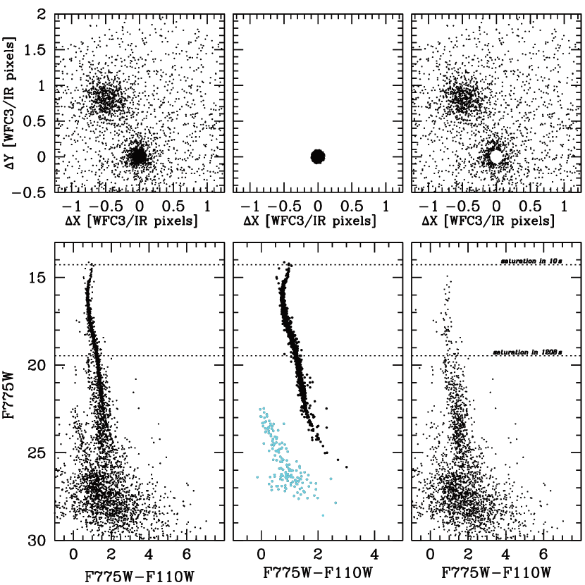
Figure 5: Top row: Vector point diagrams for all sources with counterparts with a displacement of no more than 2 WFC3/IR pixels. Bottom row: Optical-NIR ($F775W-F110W$) CMDs for all sources with optical counterparts (left); only sources with a displacement of less than 0.1 pixels, suggesting that they are cluster members (middle); and for the remaining field stars (right). The cluster CMD is used to select WDs, plotted in light blue.

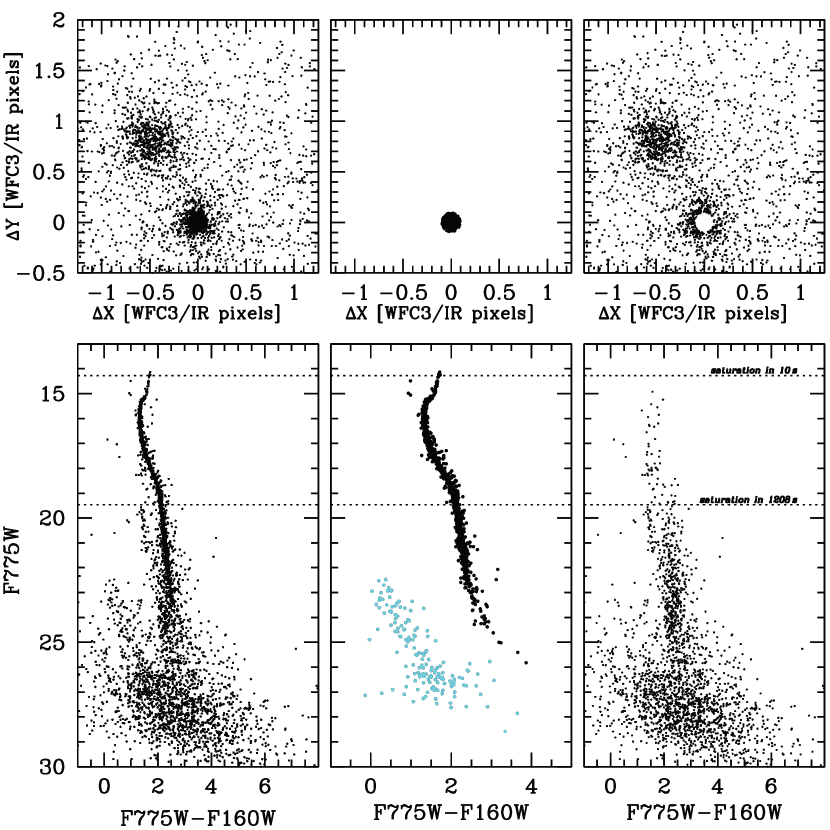
Figure 6: The same as in Fig. 5, but for $F775W-F160W$.

On the other hand, the proper-motion cleaned optical-NIR CMDs do not show any BD candidates, i.e., sources fainter than $F775W>28$ mag and redder than $F775W-F110W>3.5$ or $F775W-F160W>4.5$ mag (see also Fig. 7). This was expected, as the deep optical CMD presented in Bedin et al. (2009) did not show any potential MS sources fainter than the H-burning limit. However, and most importantly in the context of this paper, the BDs are expected to be much redder than the WDs in the optical-NIR CMDs. Indeed, the WD sequence and the MS are clearly separated in our optical-NIR CMDs. Therefore we can use the deep optical data set to identify the WDs in our NIR CMDs and disentangle WDs from potential BDs.

3.3 The minimum mass at the Hydrogen-burning limit

What is the minimum mass at the Hydrogen-burning limit in a low-metallicity cluster like M 4? And, as a consequence, at which NIR magnitude and colour do we expect the H-burning limit in our NIR CMD? Early theoretical work (Kumar 1963) suggested a lower limit to the stellar MS at $\approx 0.07M_{\odot}$ for population I and $\approx 0.09M_{\odot}$ for the metal-poor population II stars, to which also GCs belong. Hayashi & Nakano (1963) suggested that stars less massive than $0.08M_{\odot}$ cannot undergo Hydrogen burning. They further suggested that the limiting mass is not very different for Population I and Population II stars. Burrows et al. (1993) presented a zero metallicity theoretical model (i.e., Population III) which suggests a limiting H-burning mass as high as $0.094M_{\odot}$. Treatment of the atmosphere has a considerable impact on the predicted limiting mass, as can be seen in Chabrier et al. (2000) who suggested a limiting mass of $0.065M_{\odot}$ for models that include dust formation, Saumon & Marley (2008) who suggested a limiting mass of $0.075M_{\odot}$ for cloudless models, and $0.070M_{\odot}$ for cloudy models; all for solar metallicity and an age of 10 Gyr.

Previous theoretical works suggest that the H-burning limit is at higher masses for more metal-poor stars. The models roughly agree on a limiting mass of $0.075M_{\odot}$ for solar metallicities. Following Hayashi & Nakano (1963), we conservatively assume that the H-burning mass for a population as metal-poor as M 4 is between $0.075M_{\odot}$ and $0.08M_{\odot}$.

Unfortunately, detailed sub-stellar models for sub-solar metallicities are presently not available. Updated models that extend well into the BD regime are currently being computed (Allard, private communication).

However, the most recent set of BT-Settl models (Allard et al. 2012; 2013) suggest a strong metallicity dependence of the shape and luminosity of the low-mass MS. These models only go down to $0.083M_{\odot}$ and are close to the H-burning limit (Allard private communication), but do not go beyond the stellar sequence into the sub-stellar regime. Thus, we linearly extrapolated the BT-Settl models (based on the Asplund et al. 2009 solar abundances) for $\rm[M/H]=-1$ dex and an age of 12 Gyr (closest to M 4’s parameters) down to sub-stellar masses of $0.068M_{\odot}$, and applied distance and reddening as in Fig. 4 for the BT-Settl model. The extrapolated models are plotted in Fig. 7, and the magnitudes around the H-burning limit are listed in Table 1. As mentioned above, no sub-stellar models for low metallicities are currently available. Different models exist for a metallicity of $\rm{[M/H]}=0.0$ dex. Thus, in Fig. 8 we compare our extrapolated models with these more metal-rich models, all for an age of 12 Gyr and scaled to M 4’s distance and reddening. The effect of the different atmospheric physics can be clearly seen in the shape and colour of the models. However, the expected end of the H-burning sequence between a $0.075M_{\odot}$ and a $0.08M_{\odot}$ is at comparable magnitudes in all sub-stellar models. This gives us some confidence that we can use the extrapolated metal-poor BT-Settl models to get an estimate of the magnitude and colour range of the H-burning limit. For more exact values we will have to wait for the updated metal-poor models, but we remind the reader that the main purpose of this project is to provide the metal-poor benchmark sources and thereby fill the observational plane with data points that are needed to constrain theoretical models.

Unlike stars, BDs cannot retain their luminosities via nuclear fusion. As a consequence, they cool with time, and a BD will be at fainter luminosities in an old GC compared to a young BD of the same mass and metallicity. To get an estimate of this effect, we used NextGen models (Baraffe et al. 1997, Baraffe et al. 1998; see Fig. 9). In the left diagram, we plot mass against $T_{eff}$ for various ages. The right diagram shows 1 Gyr and 10 Gyr NextGen models for different metallicities. Since substellar isochrones at M 4’s low metallicity of [M/H]=-1 dex and ages of $\geq 10$ Gyr currently do not exist, we also plot isochrones for a metallicity of [M/H]=-0.5 and 0.0 dex which go down to lower masses. As can be seen, metallicity has a considerable impact on the shape of the isochrones as well as on the cooling time scale and hence fading of low-mass, substellar objects. The [M/H]=0 dex isochrones continue to extend with time to fainter magnitudes and redder colours, suggesting that a 0.075 $\rm{M}_{\odot}$ source fades by $\approx 0.7$ mag in $F110W$ from 1 to 10 Gyr, and a 0.08 $\rm{M}_{\odot}$ source becomes fainter by $\approx 0.2$ mag. The [M/H]=-0.5 dex isochrones suggest that a source of 0.079 $\rm{M}_{\odot}$ becomes fainter by $\approx 0.7$ mag, and a 0.08 $\rm{M}_{\odot}$ source becomes fainter by $\approx 0.5$ mag, but the sources also become bluer rather than redder. The [M/H]=-1 dex 10 Gyr isochrones terminates at 0.083 $\rm{M}_{\odot}$. According to the models, such a metal-poor, low-mass source already fades by 0.3 mag in $F110W$ from 1 to 10 Gyr. The models suggest that the blue-turn is more pronounced for lower-metallicities, and also metal-poor sources become fainter compared to metal-richer sources at the same mass, i.e. they cool faster.

Our optical-NIR CMDs presented in Figures 5 and 6 show that the observed MS peters out around $F775W\approx 26$ mag, suggesting that we are approaching the end of the H-burning sequence. Our NIR CMD in Fig. 4 suggests that the MS peters out just below $F110W\approx 24$ mag where the density of stars decreases. At fainter magnitudes, the WD sequence crosses the MS and the star density increases again. Based on the CMDs, we estimate our detection limits around $F775W\approx 28$ mag, $F110W\approx 26.5$ mag and $F160W\approx 27$ mag. The detection limits are also indicated in Fig. 7 with a dotted line. Comparing the theoretical models in Fig. 7 with our observed CMDs and taking the detection limits and the predicted H-burning limit into account, we conclude that we have reached beyond the H-burning limit in our NIR CMD and are probably just above or around this limit in our optical-NIR CMDs.

Table 1: Masses and corresponding magnitudes around the H-burning limit, estimated from the extrapolated BT-Settl models and scaled to M 4’s distance and reddening. All magnitudes are for HST/WFC3 filters and in the VEGAmag system.

mass [$M_{\odot}$]	$F110W$ [mag]	$F160W$ [mag]	$F775W$ [mag]
0.075	25.170	24.736	30.105
0.077	24.771	24.281	29.327
0.080	24.172	23.598	28.160

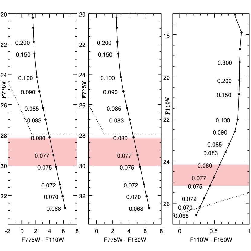
Figure 7: 12 Gyr BT-Settl models (Allard et al. 2012, 2013) in HST/WFC3 filters, scaled to M 4’s distance, reddening and metallicity. The models are extrapolated into the sub-stellar regime to 0.068 $M_{\odot}$. Masses are indicated along the sequences. The end of the H-burning sequence is estimated between 0.075 and 0.08 $M_{\odot}$ and is indicated with a light-red shaded area. Detection limits in our NIR and optical data are indicated with dotted lines. See text for further details.

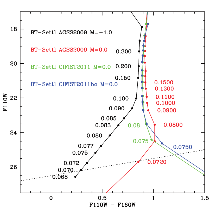
Figure 8: Comparison of our extrapolated 12 Gyr BT-Settl model with sub-stellar models at a metallicity of $\rm{[M/H]}=0.0$ dex, and with different solar abundances (AGSS2009 refers to the Asplund et al. 2009 solar abundance, CIFIST2011 was based on Caffau et al. 2011, CIFIST2011bc includes additional adjustments. See the PHOENIX webpage at https://phoenix.ens-lyon.fr/Grids/BT-Settl for more information). The different input physics are reflected in the different shapes of the models, however, the expected end of the H-burning sequence between $0.075M_{\odot}$ and a $0.08M_{\odot}$ is around $F110W\approx 24$ mag for all models.

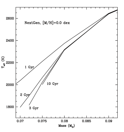
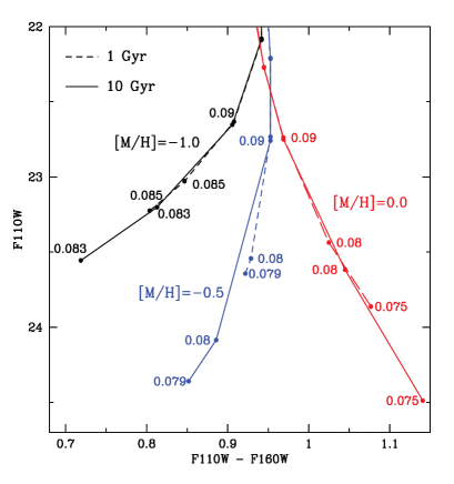
Figure 9: Low-mass stellar/BD models (NextGen) based on Baraffe et al. (1997, 1998), and Hausschildt et al. 1999. Left: Mass vs. $T_{eff}$ for 1 Gyr, 2 Gyr, 3 Gyr and 10 Gyr ([M/H]=0.0 dex). Since BDs cannot sustain their luminosities via nuclear processes, they cool with time and become fainter. Right: Low-mass isochrones that show the effect of BD cooling. The dashed line is a 1 Gyr isochrone, the solid line a 10 Gyr isochrone. Substellar models at low metallicities currently do not exist, thus isochrones for different metallicities are compared: [M/H]=-1 dex isochrones plotted in black, [M/H]=-0.5 dex in blue, [M/H]=0 dex in red. The [M/H]=-1 dex 10 Gyr isochrone terminates at 0.083 $\rm{M}_{\odot}$, suggesting that such a low-mass object already cooled and faded by 0.3 mag in $F110W$. Lower masses are available for higher metallicities, suggesting that a 0.079 $\rm{M}_{\odot}$ source fades by 0.7 mag at a metallicity of [M/H]=-0.5 dex, about the same as a 0.075 $\rm{M}_{\odot}$ source at a metallicity of [M/H]=0 dex. The models suggest that lower-mass sources cool faster the lower the mass, and also the lower the metallicity.

3.4 BD candidates

As with the best-photometry faint NIR sources, we visually inspected all cluster WD candidates, i.e., sources whose proper motion (or rather displacements) suggest that they are cluster members and whose position in the optical-NIR CMDs suggest that they are WDs. Our first photometric run on the optical data did not return an optical counterpart for 59 of the best-photometry faint NIR sources. We then over-plotted the positions of those 59 faint NIR sources (i.e., without an initial optical counterpart) on the optical $F775W$ master image and inspected each position by eye. Visual inspection of the $F775W$ master image showed a faint optical source at or close to the location of the NIR source in most cases. Thus, for the second optical photometric run (see Sect. 2.3), the parameter settings were relaxed so that all local maxima were retained, resulting in 1.5 million detections. Nearly all of those are just spurious detections (i.e., background noise or spikes in PSF wings that are not real stellar sources), however, a further 47 optical counterparts to the faint best-photometry NIR sources were detected and thus were added to the initial list of optical-NIR matches.

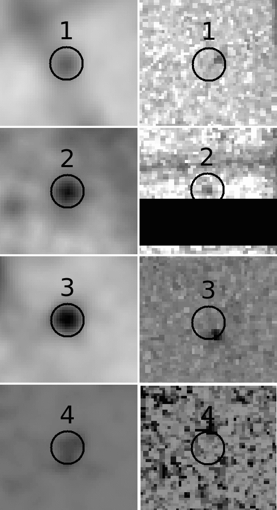
Figure 13: Zoom on the position of the 4 faint NIR sources from Table 2 in the stacked $F110W$ (left) and $F775W$ (right) images. The field of view of each image is $1.25\arcsec\times 1.25\arcsec$ and the radius of the circles is $0.15\arcsec$. North is up and East to the left.

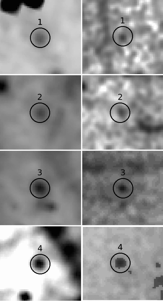
Figure 14: Zoom on the 4 WDs from Table 3 in the stacked $F110W$ (left) and $F775W$ (right) images. Orientation and field of view is the same as in Fig. 13. The WDs have similar faint NIR magnitudes than the BD candidates presented in Fig. 13, however, their optical counterpart, although faint, is clearly detectable.

For the remaining twelve faint NIR sources, still no optical counterpart was returned. However, out of those, five are located on PSF streaks and two in the ACS WFC chip gap, so that nothing can be said about an optical counterpart. For four of the remaining five sources, visual inspection of the $F775W$ master image seem to indicate an optical source on the position of the NIR source, but no photometric measurement was possible. However, we used nearby stars of similar brightness (based on pixel counts) to estimate magnitude limits. One of these sources appears to have an optical counterpart in the centre of our search circle, probably at $F775W\approx 26$ mag. This is too bright for a BD candidate and thus makes this source a WD candidate. Thus, we do not consider it further. The remaining four sources, id 1 to 4, with no optical photometry are listed in Table 2, and images are shown in Fig. 13. For comparison, we also show images of WDs selected from the proper motion cleaned CMD and which have similar NIR magnitudes to the four NIR sources without optical photometry (see Fig. 14 and Table 3).

At the rim of our search circle for source 1, an optical source can be seen. This, however, is too far away ($0\farcs 1$ away from the position of the NIR source) and would not agree with being a cluster member. In the centre of our search circle, an optical source just might be visible. If true, this source would have $F775W\gtrsim 28$ mag, i.e., the local detection limit. For source 2, an optical counterpart is visible in the centre of the search circle, again this source would be close to the detection limit at $F775W\gtrsim 28$ mag. Thus, both Source 1 and 2 are likely (massive) BD candidates. Unfortunately, Source 2 is close to a saturation streak from a nearby bright stars in the optical image. The potential counterpart, however, can be clearly distinguished. Source 3 shows a “bright” optical source at the rim of our search circle, probably at $F775W\approx 25.8$ mag, again based on the magnitudes of nearby stars that appear to be of similar brightness. However, this optical source is $0\farcs 15$ away from the position of the NIR source and thus too far away to agree with being a cluster member. A very faint optical source might just be in the centre of the search circle, if true, then this optical source would be at $F775W>28.6$ mag, the local detection limit, making source 3 a good BD candidate. Just one source, source 4, does not show an optical counterpart at the location of the NIR source (i.e., within our search circle), and is thus our best BD candidate. Since the optical photometry did not return magnitudes fainter than $F775W=32.9$ mag, an optical counterpart to BD candidate 4 must be fainter than this absolute optical limit. Note that Source 4 appears somewhat extended and could probably consist of two or three faint sources, or possibly an extended object (although we expect galaxies to be much bluer, see Bedin et al. 2009).

The positions of the four BD candidates are indicated in the CMDs in Fig. 10. Since we do not have an optical measurement, we provide the upper optical magnitude limits given in Table 2. We also overplot the extrapolated BT-Settl 12 Gyr isochrone, using the distance and reddening parameters derived from the best fit in the NIR CMD. As can be seen, all four BD candidates are very close to the extension of the MS into the BD regime, which supports our classification of these sources as good BD candidates. Source 2 is blueward of the isochrone. Its position in the optical-NIR CMDs agrees with this source being a faint WD at the very bottom of the (optical) WD cooling sequence in M 4, but it also agrees with this source being a VLMS star or a massive BD. In the NIR CMD this source is not at the very bottom of the WD sequence. We suggest that this source is a good BD candidate. Sources 1, 3 and 4 all are very close to the MS, and their position in the optical-NIR CMDs does not suggest that these sources are WDs, but rather BDs. WDs are much bluer and brighter than our BD candidates.

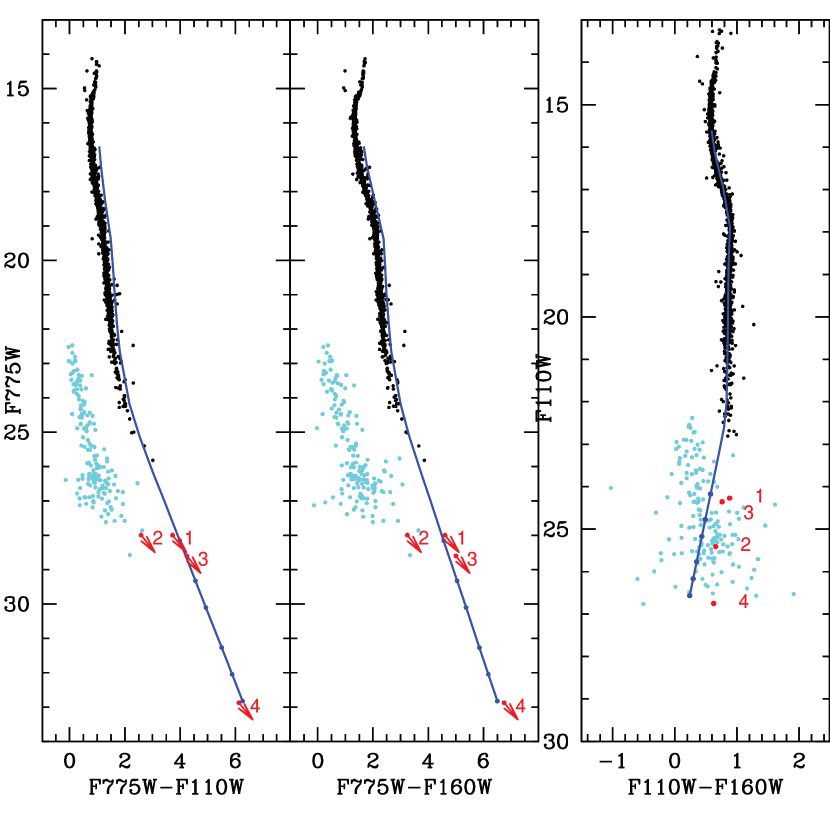
Figure 10: Optical-NIR CMDs (left and middle) and NIR CMD of all sources with an optical counterpart. We also show the position of the four BD candidates, marked with red arrows, assuming the upper optical magnitude limits given in Table 2. We also overplot the extrapolated BT-Settl 12 Gyr isochrone. As can be seen, the position of all four BD candidates is very close to the isochrone, suggesting that they are indeed BDs. See the text for more details.

Table 2: Best-photometry NIR sources fainter than $F110W>24$ mag, and for which the optical photometry did not return a counterpart. The magnitudes and errors (cols. 4 and 5) are the weighted mean and error of the weighted mean as returned from DOLPHOT. See text for further details.

idBD	RA	DEC	$F110W$	$F160W$	$F775W$	comment
	[h:m:s]	[${}^{\circ}:\arcmin:\arcsec$]	[mag]	[mag]	[mag]
1	16:23:41.701	-26:29:17.82	$24.27\pm 0.02$	$23.39\pm 0.11$	$\gtrsim$28	BD candidate
2	16:23:45.443	-26:30:05.58	$25.41\pm 0.05$	$24.75\pm 0.50$	$\gtrsim$28	WD/BD candidate
3	16:23:44.711	-26:29:30.90	$24.36\pm 0.02$	$23.60\pm 0.11$	$>28.6$	BD candidate
4	16:23:45.371	-26:29:37.40	$26.75\pm 0.16$	$26.13\pm 0.18$	$>$32.9	BD candidate

Table 3: Same as Table 2 but for WDs selected from the optical-NIR CMDs and with similar NIR magnitudes than the BD candidates. Their optical counterpart, however, is clearly detectable. The magnitudes and errors (cols. 4 to 6) are the weighted mean and error of the weighted mean as returned from DOLPHOT for the NIR, and the median-clipped mean and standard deviation for the optical magnitudes.

idWD	RA	DEC	$F110W$	$F160W$	$F775W$
	[h:m:s]	[${}^{\circ}:\arcmin:\arcsec$]	[mag]	[mag]	[mag]
1	16:23:44.354	-26:30:26.09	$25.70\pm 0.06$	$25.10\pm 0.24$	$27.184\pm 0.44$
2	16:23:36.848	-26:29:33.58	$26.30\pm 0.11$	$25.62\pm 0.40$	$27.618\pm 0.44$
3	16:23:36.953	-26:29:33.81	$25.67\pm 0.06$	$25.14\pm 0.48$	$26.607\pm 0.23$
4	16:23:47.062	-26:30:37.80	$25.68\pm 0.07$	$25.04\pm 0.37$	$26.368\pm 0.90$

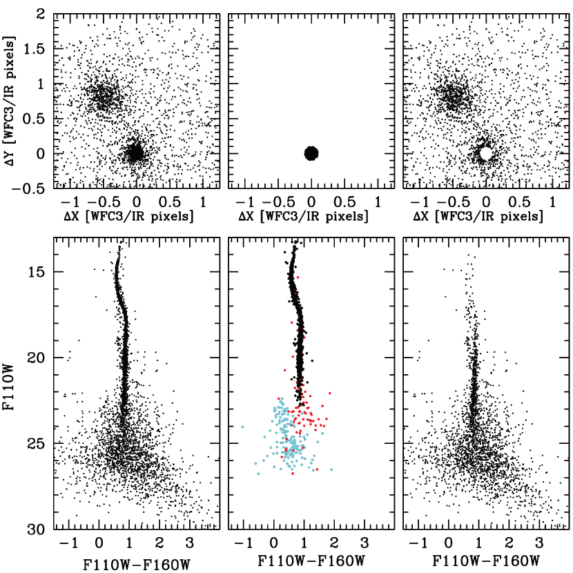
Figure 11: Top row: Vector point diagram for all sources with counterparts with a displacement of no more than 2 WFC3/IR pixels. Bottom row: NIR CMDS ($F110W$ vs. $F110W-F160W$) CMDs for all sources with optical counterparts (left); only sources with a displacement of less than 0.1 pixels, suggesting that they are cluster members (middle); and for the remaining field stars (right). The WDs selected from the optical-NIR CMDs in Figures 5 and 6 are plotted in light-blue, MS stars in black. Best-photometry NIR sources without an optical counterpart are plotted in red. As can be seen, the NIR best-photometry contains many VLMSs down to the expected H-burning limit, and reveals twelve sources around and below the expected H-burning limit ($F110W\geq 24$ mag). Out of these, one is a likely WD candidate, whereas four sources are good BD candidates. See the text for further details.

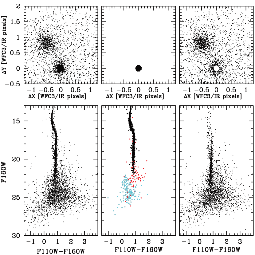
Figure 12: The same as Fig. 11, but plotted for $F160W$ vs. $F110W-F160W$.

Figures 11 and 12 again show the NIR CMDs, but only for those NIR sources for which an optical counterpart had been found (black data points). The middle CMDs show only NIR sources whose optical counterparts agree with being cluster members, based on the displacement vector point diagram. We also show best-photometry NIR sources without optical counterparts, plotted in red. As mentioned in Sect. 3.1, all 177 best-photometry NIR sources fainter than $F110W=24$ mag have been inspected on the $F110W$ and the optical $F775W$ master images. Out of these faint 177 NIR sources, 165 have an optical counterpart. Out of these 165 faint NIR/optical sources, 48 are cluster members based on their proper motion (displacements), and are located on the WD sequence. The remaining five faint best-photometry NIR sources which are not on PSF streaks or on the chip gap, and without an optical counterpart (and hence without a proper motion estimate), all make good BD candidates to start with. Visual inspection of these five sources and estimates on the optical magnitude limit (see above) suggests that one is probably a WD candidate, and the remaining four sources, listed in Table 2, are good BD candidates.

3.5 Expected number of BDs

How many BDs can we expect? This number is highly uncertain and depends on the assumed BD formation scenario (see Sect. 1). Furthermore, given our detection limits we can only expect to find the most massive BDs with masses larger than 0.068$M_{\odot}$ (based on the extrapolated BT-Settl models). Richer et al. (2004) derived a rather flat present-day mass function for M 4. Extrapolating towards fainter and lower-mass stars, they estimate that between 15 to 50 VLMSs with masses between 0.085 and 0.095 $M_{\odot}$ should be in their field of view (GO-8679, WFPC2 data). Using the theoretical models (Fig. 7) we can count the number of VLMSs in our field. If we only consider NIR sources that have an optical counterpart and a proper motion that suggests that they are cluster members, and best-photometry NIR sources without an optical counterpart, we find 23 VLMSs in a mass interval between 0.08 and 0.09 $M_{\odot}$. Assuming that the mass function is flat and that the slope of the mass function does not change considerably across the stellar/sub-stellar border, we can expect a similar number of BDs with masses between 0.070 and 0.08 $M_{\odot}$. However, the number of BDs formed per star is probably more around $\frac{1}{5}$ (see e.g. Thies et al. 2007). In this case, we can expect $\approx$ 5 BDs. This is of course a very rough estimate, but it does agree with our finding of four BD candidates.

3.6 Field contamination

How many foreground or background sources can we expect in our cluster CMD? We can simply count the number of sources that are well outside the area covered by the cluster and the clump of field stars around $\Delta Y\approx 0.75$ pixels and $\Delta X\approx-0.5$ pixels in the vector point diagram. We find a field star density of 165 field stars per $\Delta\rm{pixels}^{2}$. Scaling this number to the area covered by our cluster stars, i.e., a displacement of 0.1 WFC3 pixels, we find that we can expect 5.2 field stars in our cluster CMDs.

How many foreground stars can we then expect to have NIR magnitudes and colours similar to our BD candidates? Selecting only field stars with $24<F110W<27$ mag and $0<F110W-F160W<1$ mag, the field star density is reduced to 50 stars/$\Delta\rm{pixels}^{2}$, and scaled to the area covered by the cluster in the vector point diagram , we then find that 1.6 such sources can be expected among our pm selected faint cluster members. Thus, about half of our suggested BD candidates might actually be foreground or background sources that happen to move with the cluster velocity across the plane of the sky.

4 Summary and Conclusion

We have presented the deepest NIR HST/WFC3 study of the GC M 4 to date. The NIR data were proper-motion cleaned using archival deep optical HST/ACS ($F775W$) data. Our best-photometry NIR CMD reveals a narrow MS delineating down towards the expected end of the H-burning sequence. 177 best-photometry NIR sources fainter than the H-burning limit in $F110W$ ($F110W>24$ mag) could be identified in our $F110W$ master image. For 165 of these faint NIR sources, an optical counterpart was found, 48 of these are cluster members according to their proper motion. All of these 48 faint cluster sources are on the WD sequence.

We found in total five faint NIR sources for which the optical photometry did not return a measurement (and which are not on PSF streaks or on the chip gap). We then visually inspected the positions of these faint NIR sources on the optical images and estimated, where possible, upper optical magnitude limits of potential optical counterparts that just might be visible. One source is likely another WD and rejected as a BD candidate. Based on the upper optical magnitude limits, we indicate the position of the remaining four sources in the optical-NIR CMDs. One of the sources (source 4 in Table 2), does not show an optical counterpart at all, which implies that its optical counterpart must be fainter than the absolute optical detection limit of $F775W>32.9$ mag. This source appears to be somewhat extended in the NIR image, which might indicate multiple faint sources, i.e. multiple BDs, or possibly a galaxy. However, its position in the CMDs does agree with this source being a BD. One source (source 2 in Table 2) might be another WD candidate, but its position in the optical-NIR CMD also agrees with this source being a massive BD or a VLMS star at the bottom of the MS. The remaining two sources also have positions that indicate that these sources are massive BDs. We conclude that we have found four good BD candidates, but we caution that further studies and deeper optical data are necessary to confirm their status and cluster membership.

References

- Allard et al. (2012) Allard F., Homeier D. & Freytag B. 2012, RSPTA, 370, 2765
- Allard et al. (2013) Allard F., Homeier D. & Freytag B. 2013, MmSAI, 84, 1053
- Anderson et al. (2008) Anderson J., Sarajedini A., Bedin L. R., King I. R., Piotto G. et al. 2008, AJ, 135, 2055
- Anderson & Bedin (2010) Anderson J. & Bedin L. R. 2010, PASP, 122, 1035
- Asplund et al. (2009) Asplund M., Grevesse N., Sauval A. J. & Scott P. 2009, ARA&A, 47, 481
- André et al. (2012) André P, Ward-Thompson D. & Greaves J. 2012, Science, 337, 69
- Baraffe et al. (1997) Baraffe, I., Chabrier, G., Allard, F., & Hauschildt, P. H. 1997, A&A, 327, 1054
- Baraffe et al. (1997) Baraffe, I., Chabrier, G., Allard, F., & Hauschildt, P. H. 1998, A&A, 337, 403
- Barber et al. (2006) Barber R. J., Tennyson J., Harris G. J. & Tolchenov R. N. 2006, MNRAS, 368, 1087
- Basu & Vorobyov (2012) Basu S. & Vorobyov E. I. 2012, ApJ, 750, 30
- Beer et al. (2004) Beer M. E., King A. R. & Pringle J. E. 2004, MNRAS, 355, 1244
- Bedin et al. (2001) Bedin L. R., Anderson J., King I. R., Piotto G. 2001, ApJ, 560L, 75
- Bedin et al. (2003) Bedin L. R., Giampaolo P., King I. R. & Anderson J. 2003, AJ, 126, 247
- Bedin et al. (2009) Bedin L. R., Salaris M., Piotto G., Anderson J., King I. R., Cassisi S. 2009, ApJ, 697, 965
- Boudreault & Lodieu (2012) Boudreault S. & Lodieu N. 2013, MNRAS, 434, 142
- Braga et al. (2015) Braga V. F., Dall’Ora M., Bono G., Stetson P. B., Ferraro I. et al. 2015, ApJ, 799, 165
- Burgasser et al. (2003) Burgasser A. J., Kirkpatrick J. D., Burrows A., Liebert J., Reid I. N., Gizis J. E., McGovern M. R., Prato L., McLean I. S. 2003 ApJ, 592, 1186
- Burgasser & Kirkpatrick (2006) Burgasser A. J. & Kirkpatrick J. D. 2006, ApJ, 645, 1485
- Burgasser et al. (2009) Burgasser A. J., Witte S., Helling C., Sanderson R. E., Bochanski J. J., Hauschildt P. H. 2009, ApJ, 697, 148
- Burningham et al. (2014) Burningham B., Smith L., Cardoso C. V., Lucas P. W., Burgasser A. J., Jones H. R. A., Smart R. L., 2014, MNRAS, 440, 359
- Burrows et al. (1993) Burrows A., Hubbard W. B., Saumon D. & Lunine J. I. 1993, ApJ, 406, 158
- Burrows et al. (1997) Burrows A., Marley M. Hubbard W. B. et al. 1997, ApJ, 491, 856
- Burrows et al. (2001) Burrows A., Hubbard W. B., Lunine J. I. & Liebert J. 2001, Reviews of Modern Physics, 73, 719
- Caffau et al. (2009) Caffau E., Maiorca E., Bonifacio P., Faraggiana R., Steffen M. et. al. 2009, A&A, 498, 877
- Casewell et al. (2014) Casewell S. L., Littlefair S. P., Burleigh M. R. & Roy M. 2014, MNRAS, 441, 2644
- Chabrier et al. (2000) Chabrier G., Baraffe I., Allard F. & Hauschildt P. H. 2000, ApJ, 542, 464
- Cushing et al. (2009) Cushing M. C., Looper D., Burgasser A. J., Kirkpatrick J. D., Faherty J. et al. 2009, ApJ, 696, 986
- Dolphin (2000) Dolphin 2000, PASP, 112, 1383
- Dotter et al. (2008) Dotter A., Chaboyer B., Jevremovic D., Kostov V., Baron E., Ferguson J. W. 2008, ApJS, 178, 89
- Elmegreen (1999) Elmegreen B. G. ApJ, 1999, 522, 915
- Fischer & Valenti (2005) Fischer D. A. & Valenti J. 2005, ApJ, 622, 1102
- Gänsicke et al. (1995) Gänsicke B., Beuermann K. & de Martino D. 1995, A&A, 303, 127
- Hansen et al. (2004) Hansen B. M. S., Richer H. B., Fahlman G. G., Stetson P. B., Brewer J. et al. 2004, ApJS, 155, 551
- Harris (1996) Harris W.E. 1996, AJ, 112, 1487
- Hasegawa & Hirashita (2014) Hasegawa, Y. & Hirashita, H. 2014, ApJ, 788, 62
- Hayashi & Nakano (1963) Hayashi, C. & Nakano, T. 1963, Progress of Theoretical Physics, 30, 460
- Hendricks et al. (2012) Hendricks B., Stetson P. B., VandenBerg D. A. & Dall’Ora M. 2012, AJ, 144, 25
- Kaplan et al. (2012) Kaplan M., Stramatellos D. & Whitworth A. P. 2012, Ap&SS. 341, 395
- Kirkpatrick et al. (2014) Kirkpatrick J. D., Schneider A., Fajardo-Acosta S., Gelino C. R., Mace G. N. et al. 2014, ApJ, 783, 122
- Krist et al. (2011) Krist J. E., Hook R. N. & Stoehr F. 2011, Proceedings of the SPIE, Volume 8127, id. 81270J
- Kroupa & Bouvier (2003) Kroupa P. & Bouvier J. 2003, MNRAS, 346, 369
- Kumar (1963) Kumar S. S. 1963, ApJ, 137, 1121
- Lépine et al. (2004) Lépine S., Shara M. M. & Rich R. M. 2004, ApJL, 602, 125
- Lawrence et al. (2007) Lawrence A., Warren S. J., Almaini O., Edge A. C., Hambly N. C. et al. 2007, MNRAS, 379, 1599
- Luhman & Sheppard (2014) Luhman K. L. & Sheppard S. S. 2014, ApJ, 787, 126
- Mace et al. (2013) Mace G. N, Kirkpatrick J. D., Cushing M. C., Gelino C. R., McLean I. S. et al. 2013, ApJ, 777, 36
- Malavolta et al. (2014) Malavolta L., Sneden C., Piotto G., Milone A. P., Bedin L. R. & Nascimbeni V. 2014, ApJ, 147, 25
- Martín et al. (2001) Martín E. L., Dougados C., Magnier E. Ménard F., Magazzù A., Cuillandre J.-C., Delfosse X. 2001, ApJ, 561, 195
- Milone et al. (2012) Milone A. P., Piotto G., Bedin L. R., Aparicio A., Anderson J. et al. 2012, A&A, 540, 16
- Milone et al. (2014) Milone A. P., Marino A. F., Bedin L. R., Piotto G., Cassisi S., Dieball A. et al. 2014, MNRAS, 439, 1588
- Murray et al. (2011) Murray D. N., Burningham B., Jones H. R. A., Pinfield D. J., Lucas P. W. et al. 2011, MNRAS, 414, 575
- Pinfield et al. (2003) Pinfield D. J., Dobbie P. D., Jameson R. F., Steele I. A., Jones H. R. A., Katsiyannis A. C. 2003, MNRAS, 342, 1241
- Pinfield et al. (2014) Pinfield D. J., Gomes J., Day-Jones A. C., Leggett S. K., Gromadzki M. et al. 2014, MNRAS, 437, 1009
- Rebolo et al. (1996) Rebolo R., Martin E. L., Basri G., Marcy G. W. & Zapatero-Osorio M. R. 1996, ApJ, 469, 53
- Reipurth & Clarke (2001) Reipurth B. & Clarke C. 2001, AJ, 122, 432
- Richer et al. (1997) Richer H. B., Fahlman G. G., Ibata R. A. et al. 1997, ApJ, 484, 741
- Richer et al. (2004) Richer H. B., Brewer J., Fahlman G. G., Kalirai J., Stetson P. B., Hansen B. M. S., Rich R. M., Ibata R. A., Gibson B. K., Shara, M. 2004, AJ, 127, 2904
- Sarajedini et al. (2007) Sarajedini A., Bedin L. R., Chaboyer B., Dotter A., Siegel M. et al. 2007, AJ, 133, 1658
- Saumon & Marley (2008) Saumon D. & Marley M. S. 2008, ApJ, 689, 1327
- Seaton (1979) Seaton, M. J. 1979, MNRAS, 187, 785
- Sigurdsson et al. (2003) Sigurdsson S., Richer H. B., Hansen B. M., Stairs I. H., Thorsett S. E. 2003, Science, 301, 193
- Sivarani et al. (2009) Sivarani T., Lépine S., Kambhavi A. K. & Gupchup J. 2009, ApJL, 694, 140
- Skrutskie et al. (2006) Skrutskie M., Cutri R. M., Stiening R., Weinberg M. D., Schneider S. et al. 2006, AJ, 131, 1163
- Stamatellos et al. (2011) Stamatellos D., Maury A., Whitworth A. & André 2011, MNRAS, 413, 1787
- Stamatellos (2014) Stamatellos D. 2014, ASSP, 36, 17
- Steele et al. (1995) Steele I. A., Jameson R. F., Hodgkin S. T. & Hambly N. C. 1995. MNRAS, 275, 841
- Thies & Kroupa (2007) Thies I. & Kroupa P. 2007, ApJ, 671, 767
- Thies et al. (2010) Thies I., Kroupa P., Goodwin S., Stamatellos D., Whitworth A. 2010 ApJ, 717, 577
- Thies et al. (2015) Thies I., Pflamm-Altenburg J., Kroupa P. & Marks M. 2015, ApJ accepted, arXiv:1501.01640
- Whitworth & Goodwin (2005) Whitworth A. P. & Goodwin S. P. 2005, AN, 326, 899
- Wright et al. (2010) Wright E. L., Eisenhardt P. R. M., Mainzer A. K., Ressler M. E., Cutri R. M. et al. 2010, AJ, 140, 1868
- Wood (1995) Wood, M. A. 1995, in White Dwarfs, ed. D. Koester & K. Werner (Berlin: Springer), 41
- York et al. (2000) York D. G., Adelman J., Anderson J. E., Anderson S. F., Annis J. et al. 2000, AJ, 120, 1579
- Zloczewski et al. (2012) Zloczewski K., Kaluzny J., Rozyczka M., Krzeminski W., Mazur B. & Thompson I. B. 2012, Acta Astronomica, 62, 357