A Double AR Model Without Intercept: an Alternative to Modeling Nonstationarity and Heteroscedasticity

Abstract

This paper presents a double AR model without intercept (DARWIN model) and provides us a new way to study the non-stationary heteroskedastic time series. It is shown that the DARWIN model is always non-stationary and heteroskedastic, and its sample properties depends on the Lyapunov exponent. An easy-to-implement estimator is proposed for the Lyapunov exponent, and it is unbiased, strongly consistent and asymptotically normal. Based on this estimator, a powerful test is constructed for testing the stability of the model. Moreover, this paper proposes the quasi-maximum likelihood estimator (QMLE) for the DARWIN model, which has an explicit form. The strong consistency and asymptotical normality of the QMLE are established regardless of the sign of the Lyapunov exponent. Simulation studies are conducted to assess the performance of the estimation and testing and an empirical example is given for illustrating the usefulness of the DARWIN model.

Key words: DAR model; DARWIN model; Geometric Brownian motion; Heteroscedasticity; Lyapunov exponent; Non-stationary time series; Quasi-maximum likelihood estimation; Stability.

1 Introduction

Time-varying volatility has been crucial in modeling economic and financial time series. Since the seminal work of Engle (1982), the autoregressive conditional heteroscedasticity (ARCH) model and its numerous variants have been widely used; see, e.g., Bollerslev et al. (1992) and Francq and Zakoïan (2010). Among them, the first order double autoregressive (DAR) model has attracted much attention, which takes the form

$$y_{t}=\phi_{0}y_{t-1}+\eta_{t}\sqrt{\omega_{0}+\alpha_{0}y_{t-1}^{2}},$$ (1.1)

where $\phi_{0}\in(-\infty,\infty)$, $\omega_{0}\geq 0$, $\alpha_{0}\geq 0$, $\{\eta_{t}\}$ is a sequence of independent and identically distributed (i.i.d.) random variables with zero mean and unit variance, and $\eta_{t}$ is independent of $\{y_{j};j<t\}$. Model (1.1) was initially introduced by Weiss (1984), and the term ‘double autoregressive’ was coined by Ling (2004) since both the conditional mean and variance functions are regressions only on the observed data and its square, respectively. Clearly, model (1.1) belongs to the class of ARMA-ARCH models in Weiss (1984) and of nonlinear AR models in Cline and Pu (2004), but it is different from Engle’s ARCH model if $\phi_{0}\neq 0$. Its higher-order extension and generalization can be found in Weiss (1984), Lu (1998), Ling (2007), Zhu and Ling (2013), Guo, Ling and Zhu (2014), Li, Ling and Zakoïan (2015), Li, Ling and Zhang (2015) and many others.

The stationarity conditions and the associate inferential theory of model (1.1) have been well studied under the compact parameter space $\Lambda=\{\lambda_{0}=(\phi_{0},\omega_{0},\alpha_{0}):|\phi_{0}|\leq\bar{\phi},\underline{\omega}\leq\omega_{0}\leq\bar{\omega},\underline{\alpha}\leq\alpha_{0}\leq\bar{\alpha}\}$, where $\bar{\phi}$, $\underline{\omega}$, $\bar{\omega}$, $\underline{\alpha}$ and $\bar{\alpha}$ are some finite positive constants. Early contributions in this context include Gu$\acute{e}$gan and Deibolt (1994) and Borkovec and Kl$\ddot{u}$ppelberg (2001), who derived the sufficient and necessary condition of weak stationarity of model (1.1). Recently, Chen, Li and Ling (2014) proved that when $\eta_{t}$ is symmetric, model (1.1) is strictly stationary if and only if the Lyapunov exponent $\gamma_{0}=E\log|\phi_{0}+\eta_{t}\sqrt{\alpha_{0}}|<0$.

By assuming that the true value $\lambda_{0}$ is an interior point of $\Lambda$, the inference of model (1.1) based on quasi-maximum likelihood estimation exhibits quite different phenomenon in terms of $\gamma_{0}$. For instance, when $\gamma_{0}<0$, Ling (2004) showed that the quasi-maximum likelihood estimator (QMLE) of $\lambda_{0}$ is consistent and asymptotically normal; and when $\gamma_{0}\geq 0$, Ling and Li(2008) and Chen, Li and Ling (2014) demonstrated that the (unconstrained) QMLE of $(\phi_{0},\alpha_{0})$ is consistent and asymptotically normal, but the intercept term $\omega_{0}$ cannot be consistently estimated. This phenomenon can also be found for the least absolute deviation estimator and robust quasi-maximum likelihood estimation in Chan and Peng (2005), Zhu and Ling (2013), and Li, Guo, and Li (2015).

In all aforementioned work, the positivity of $\omega_{0}$ is essential for the strict stationarity and (robust) quasi-maximum likelihood estimation, although the intercept $\omega_{0}$ is not involved directly in $\gamma_{0}$. The case that $\omega_{0}=0$ would be meaningful but hardly touched so far. As one motivation of this paper, it is of interest to fill in this gap from a theoretical viewpoint. Another parallel motivation of this study is from application. The importance of model (1.1) and its higher-order extension has been well demonstrated by empirical studies; see, e.g., Ling (2004), Zhu and Ling (2013), and many others. In these applications, however, an interesting finding is that the intercept term $\omega_{0}$ is often very close to zero; see also the illustrating example in Section 6 below. As a result, it is intuitively appealing to study a first-order double AR model without intercept (abbreviated to DARWIN(1)) as follows:

$$y_{t}=\phi_{0}y_{t-1}+\eta_{t}\sqrt{\alpha_{0}y_{t-1}^{2}},$$ (1.2)

where all notations inherit from model (1.1) with $\alpha_{0}>0$. In the special case of $\phi_{0}=0$, model (1.2) becomes the ARCH model without intercept in Hafner and Preminger (2015). In this paper, we are concerned with the probability structure of model (1.2) and the estimation and inference of $\gamma_{0}$ and $(\phi_{0},\alpha_{0})$. It is surprising that its probabilistic structures and asymptotics of the QMLE are totally different from those of model (1.1). This is out of our expectation. Moreover, model (1.2) is always non-stationary and heteroskedastic regardless of the sign of $\gamma_{0}$, and hence it provides us a new way to model the non-stationary heteroskedastic time series. Specifically, it can be seen that when $\gamma_{0}=0$, the conditional volatility of $y_{t}$ is a nondegenerate random variable oscillating randomly between zero and infinity over time, while when $\gamma_{0}\not=0$, this is not the case. In this sense, model (2) is stable if $\gamma_{0}=0$, and unstable otherwise; see also Hafner and Preminger (2015) for the same argument in the ARCH model without intercept.

This paper is organized as follows. Section 2 considers sample path properties of $y_{t}$ in model (1.2). Section 3 proposes a new estimator of $\gamma_{0}$ and discusses its asymptotic theory and also a test for stability. Section 4 focuses on the QMLE of $(\phi_{0},\alpha_{0})$ in model (1.2) and derives its asymptotic properties. Sections 5 and 6 investigate the numerical properties of the proposed procedures using both simulated and real data. The conclusions are offered in Section 7. All technical proofs are relegated to the Appendix.

2 Sample path properties

In this section, we study sample path properties of $y_{t}$ in model (1.2), when $\eta_{t}$ is symmetric but not necessarily has mean zero and variance one. To accomplish it, we consider an auxiliary process

$$x_{t}=\Big{|}\phi_{0}x_{t-1}+\eta_{t}\sqrt{\alpha_{0}x^{2}_{t-1}}\Big{|},$$ (2.1)

where the initial value $x_{0}=|y_{0}|$. It is straightforward to see that

$$x_{t}=|\phi_{0}+\eta_{t}\sqrt{\alpha_{0}}|x_{t-1}\quad\mbox{or}\quad\log x_{t}=\log|\phi_{0}+\eta_{t}\sqrt{\alpha_{0}}|+\log x_{t-1}.$$ (2.2)

Note that when $\eta_{t}$ is symmetric, it is readily seen that

$$\{x_{t}\}\stackrel{{\scriptstyle d}}{{=}}\{|y_{t}|\};$$ (2.3)

see, e.g., Borkovec (2000) and Borkovec and Kl$\ddot{u}$ppelberg (2001). Thus, $|y_{t}|$ either converges to zero or diverges to infinity almost surely at an exponential rate as $t\rightarrow\infty$, according to $\gamma_{0}<0$ or $\gamma_{0}>0$, respectively. This result sharply differs from the one in model (1.1) when $\gamma_{0}<0$.

Next, we precisely characterize asymptotic distribution of $|y_{t}|$ after a suitable renormalization. Let $[a]$ be the integral part of any real number $a$. The expression (2.2) implies that for any $s\in[0,1]$,

$$\frac{1}{\sqrt{n}}\log\frac{x_{[ns]}}{\exp\{[ns]\gamma_{0}\}}=\frac{1}{\sqrt{n}}\sum_{i=1}^{[ns]}(\log|\phi_{0}+\eta_{i}\sqrt{\alpha_{0}}|-\gamma_{0})+\frac{1}{\sqrt{n}}\log x_{0}.$$

By (2.3) and Donsker’s Theorem in Billingsley (1999, p.90), we have the following theorem:

Theorem 2.1. Suppose that $\{\eta_{t}\}$ is a sequence of i.i.d. symmetric random variables satisfying $\sigma_{\gamma_{0}}^{2}=\mathrm{var}(\log|\phi_{0}+\eta_{t}\sqrt{\alpha_{0}}|)\in(0,\infty)$. If $y_{0}$ is symmetric with $P(y_{0}=0)=0$, and independent of $\{\eta_{t}:t\geq 1\}$, then

$$\frac{|y_{{[ns]}}|^{\frac{1}{\sqrt{n}}}}{\exp(s\gamma_{0}\sqrt{n})}\Longrightarrow\exp\{\sigma_{\gamma_{0}}\mathbb{B}(s)\}\quad\mbox{as $n\rightarrow\infty$ \quad in $\mathbb{D}[0,1]$},$$

where ‘$\Longrightarrow$’ denotes weak convergence, $\mathbb{B}(s)$ is a standard Brownian motion on $[0,1]$, and $\mathbb{D}[0,1]$ is the space of functions defined on $[0,1]$, which are right continuous and have left limits, endowed with the Skorokhod topology.

Figure 1: One sample path of $\{y_{t}\}_{t=1}^{100}$ in model (1.2) corresponding to $\gamma_{0}<0$, $\gamma_{0}=0$, and $\gamma_{0}>0$, respectively.

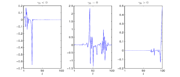
Theorem 2.1 has many implications. First, it implies that $y_{t}$ is non-stationary and heteroskedastic regardless of the sign of $\gamma_{0}$. Second, its sample path property depends on the sign of $\gamma_{0}$. Precisely, it indicates that, if $\gamma_{0}=0$, the conditional volatility of $y_{t}$ is a nondegenerate random variable oscillating randomly between zero and infinity over time; otherwise, $|y_{t}|$ either converges to zero or diverges to infinity almost surely (a.s.) as $t\to\infty$. To illustrate this, we present one sample path of $\{y_{t}\}$ of model (1.2) with $\eta_{t}\sim N(0,1)$, $\phi_{0}=0.5$, and $\alpha_{0}=3.1$ (i.e., $\gamma_{0}<0$), 3.3058 (i.e., $\gamma_{0}=0$), or 3.5 (i.e., $\gamma_{0}>0$). The plots are depicted in Fig.1. They show clear evidence of different sample path properties with various $\gamma_{0}$. To distinguish them, model (1.2) is called stable if $\gamma_{0}=0$, and unstable otherwise; see Hafner and Preminger (2015) for the same argument in the ARCH model without intercept. Since $\gamma_{0}$ plays a key role in determining the stability of model (1.2), it is desirable to consider its estimation and inference in the next section.

3 Estimation of Lyapunov exponent

In this section, we propose a simple estimator for $\gamma_{0}$. This estimator requires only the data $y_{n}$ and $y_{0}$ but shares good properties. As in Section 2, we assume that $\eta_{t}$ is symmetric and not necessarily has mean zero and variance one. The basic idea is very intuitive. By (2.1), we have $\log(x_{t}/x_{t-1})=\log|\phi_{0}+\eta_{t}\sqrt{\alpha_{0}}|$, and then

$$\frac{1}{n}(\log x_{n}-\log x_{0})=\frac{1}{n}\sum_{t=1}^{n}\log(x_{t}/x_{t-1})=\frac{1}{n}\sum_{t=1}^{n}\log|\phi_{0}+\eta_{t}\sqrt{\alpha_{0}}|\to\gamma_{0}\,\,\,\mbox{ a.s.}$$

provided that $\gamma_{0}<\infty$. Consequently, an easy-to-implement estimator of $\gamma_{0}$ is defined by

$$\widehat{\gamma}_{n}=\frac{1}{n}(\log|y_{n}|-\log|y_{0}|).$$

The following theorem states that $\widehat{\gamma}_{n}$ is unbiased and asymptotically normal.

Theorem 3.1. If the assumptions in Theorem 2.1 hold, then, $\mathrm{(i)}$ $\widehat{\gamma}_{n}$ is unbiased; $\mathrm{(ii)}$ $\widehat{\gamma}_{n}\rightarrow\gamma_{0}$ a.s.; and $\mathrm{(iii)}$ $\sqrt{n}(\widehat{\gamma}_{n}-\gamma_{0})\Longrightarrow N(0,\sigma^{2}_{\gamma_{0}})$ as $n\rightarrow\infty$, where $\sigma^{2}_{\gamma_{0}}$ is defined as in Theorem 2.1.

As an application, consider a testing problem whether model (1.2) is stable or not, i.e.,

$$H_{0}:\gamma_{0}=0\quad\mbox{v.s.}\quad H_{1}:\gamma_{0}\neq 0.$$

Based on Theorem 3.1, the proposed test statistic is given by

$$T_{n}=\sqrt{n}\frac{\widehat{\gamma}_{n}}{\widehat{\sigma}_{\gamma}},$$ (3.1)

where $\widehat{\sigma}^{2}_{\gamma}=\tfrac{1}{n}\sum_{t=1}^{n}\{\log(|y_{t}|/|y_{t-1}|)\}^{2}-\widehat{\gamma}_{n}^{2}$. Under $H_{0}$, it is not hard to prove that $T_{n}\Longrightarrow N(0,1)$ as $n\to\infty$. Thus, $H_{0}$ is rejected at the significance level $\beta\in(0,1)$ when $|T_{n}|>\Phi^{-1}(\beta/2)$, where $\Phi(\cdot)$ is the cumulative distribution function of $N(0,1)$.

4 Quasi-maximum likelihood estimation

Let $\theta=(\phi,\alpha)^{\mathrm{\scriptscriptstyle T}}$ be the unknown parameter of model (1.2) with true value $\theta_{0}=(\phi_{0},\alpha_{0})^{\mathrm{\scriptscriptstyle T}}$. Denote the parameter space by $\Theta=\mathcal{R}\times(0,\infty)$. Assume that $\{y_{1},\cdots,y_{n}\}$ are generated by model (1.2). When $\eta_{t}\sim N(0,1)$, the log-likelihood function (ignoring a constant) can be written as

$$L_{n}(\theta)=\sum_{t=1}^{n}l_{t}(\theta)\quad\mbox{ with }\quad\ell_{t}(\theta)=-\frac{1}{2}\left\{\log(\alpha y_{t-1}^{2})+\frac{(y_{t}-\phi y_{t-1})^{2}}{\alpha y_{t-1}^{2}}\right\}.$$

Then, the quasi-maximum likelihood estimator (QMLE) of $\theta_{0}$ is defined as

$$\widehat{\theta}_{n}:=(\widehat{\phi}_{n},\widehat{\alpha}_{n})^{\mathrm{\scriptscriptstyle T}}=\arg\max_{\theta\in\Theta}L_{n}(\theta).$$

By setting $\partial L_{n}(\theta)/\partial\theta=0$, it is not hard to see that $\widehat{\theta}_{n}$ has a unique explicit expression with

$$\widehat{\phi}_{n}=\frac{1}{n}\sum_{t=1}^{n}\frac{y_{t}}{y_{t-1}}\quad\mbox{ and }\quad\widehat{\alpha}_{n}=\frac{1}{n}\sum_{t=1}^{n}\frac{(y_{t}-\widehat{\phi}_{n}y_{t-1})^{2}}{y_{t-1}^{2}}.$$

With the help of this explicit expression, it is convenient to obtain the asymptotic properties of $\widehat{\theta}_{n}$ in the following theorem.

Theorem 4.1. Suppose that $E\eta_{t}=0$ and $E\eta_{t}^{2}=1$. Then,

$\mathrm{(i)}$ $\widehat{\phi}_{n}$ is unbiased, but $\widehat{\alpha}_{n}$ is asymptotically unbiased;

$\mathrm{(ii)}$ $\widehat{\theta}_{n}\rightarrow\theta_{0}$ a.s. as $\rightarrow\infty$;

$\mathrm{(iii)}$ Furthermore, if $E\eta_{t}^{3}=0$ and $\kappa_{4}=E\eta_{t}^{4}<\infty$, then

$$\sqrt{n}(\widehat{\theta}_{n}-\theta_{0})\Longrightarrow N(0,\Sigma)$$

as $n\rightarrow\infty$, where $\Sigma=\mathrm{diag}(\alpha_{0},(\kappa_{4}-1)\alpha_{0}^{2})$.

Remark 4.1. In Theorem 4.1 (i) and (ii), the symmetric condition of $\eta_{t}$ is not required but we need one more condition that $E\eta_{t}^{3}=0$ for part (iii) of this theorem. This is to guarantee the existence of covariance $\Sigma$. From the proof of this theorem, we have

$$\lim_{n\to\infty}\mathrm{cov}(\sqrt{n}(\widehat{\phi}_{n}-\phi_{0}),\sqrt{n}(\widehat{\alpha}_{n}-\alpha_{0}))=\alpha_{0}^{3/2}E\eta_{t}^{3}\times\left[\lim_{n\to\infty}\frac{1}{n}\sum_{t=1}^{n}E[\mbox{sign}(y_{t-1})]\right];$$

since $y_{t}$ is non-stationary, the limit in the proceeding equation may not exist unless $E\eta_{t}^{3}=0$.

Remark 4.2. Although $\widehat{\alpha}_{n}$ is biased, its re-scaled version $\widehat{\alpha}^{*}_{n}=\frac{n}{n-1}\widehat{\alpha}_{n}$ is unbiased.

Remark 4.3. Compared to the asymptotic property of the QMLE in Ling (2004) and Chen, Li and Ling (2014), Theorem 4.1 has two interesting features. First, the compactness of the parameter space $\Theta$ is not necessary. Second, the asymptotic covariances of $\widehat{\theta}_{n}$ are the same in both the stable and unstable cases.

Remark 4.4. As a possible application of Theorem 4.1, one may consider a natural plug-in estimator of $\gamma_{0}$ as $\widehat{\gamma}_{n}^{*}=\frac{1}{n}\sum_{t=1}^{n}\log\big{|}\widehat{\phi}_{n}+\widehat{\eta}_{t}\sqrt{\widehat{\alpha}_{n}}\big{|}$, where $\widehat{\eta}_{t}=(y_{t}-\widehat{\phi}_{n}y_{t-1})/\sqrt{\widehat{\alpha}_{n}y_{t-1}^{2}}$ is the residual of model (1.2). However, unlike Francq and Zakoïan (2012), the asymptotic normality of $\widehat{\gamma}_{n}^{*}$ requires that $E\{(\phi_{0}+\eta_{t}\sqrt{\alpha_{0}})^{-1}\}<\infty$, which does not exist generally, even for $\eta_{t}$ being standard normal. See also Li, Guo and Li (2015) for more relevant discussions.

To construct confidence intervals for $\theta_{0}$, we need to estimate $\kappa_{4}$. Define $\widehat{\kappa}_{n}=\frac{1}{n}\sum_{t=1}^{n}\widehat{\eta}_{t}^{\,4}$. By a simple calculation, we can show that $\widehat{\kappa}_{n}\rightarrow\kappa_{4}$ a.s. as $n\to\infty$. Moreover, by letting $\widehat{\Sigma}_{n}=\mathrm{diag}(\widehat{\alpha}_{n},(\widehat{\kappa}_{n}-1)\widehat{\alpha}_{n}^{2})$, we can construct a Wald test statistic

$$W_{n}=n(\Gamma\widehat{\theta}_{n}-r)^{\mathrm{\scriptscriptstyle T}}(\Gamma\widehat{\Sigma}_{n}\Gamma^{\mathrm{\scriptscriptstyle T}})^{-1}(\Gamma\widehat{\theta}_{n}-r)$$

to detect the linear null hypothesis $H_{0}:\Gamma\theta_{0}=r$, where $\Gamma\in\mathcal{R}^{s\times 2}$ is a constant matrix with rank $s$ and $r\in\mathcal{R}^{s\times 1}$ is a constant vector. At the significance level $\beta\in(0,1)$, we reject $H_{0}$ if $W_{n}>\Psi_{s}^{-1}(1-\beta)$, where $\Psi_{d}(\cdot)$ is the cumulative distribution function of $\chi^{2}_{d}$. Otherwise, $H_{0}$ is not rejected.

To end this section, we offer some discussions on the model checking. In the context of non-stationary time series, Ling et al.(2013) considered two portmanteau tests for non-stationary ARMA models, where one is based on the residual autocorrelation functions (ACFs) as in Ljung and Box (1978), and the other is based on the squared residual ACFs as in McLeod and Li (1983). However, their methods are hard to be implemented for model (1.2). To see it clearly, define the lag-$k$ residual ACF of $\{\widehat{\eta}_{t}\}$ as

$$\breve{\rho}_{k}^{\,*}=\frac{\sum_{t=k+1}^{n}(\widehat{\eta}_{t}-\overline{\eta_{n}^{*}})(\widehat{\eta}_{t-k}-\overline{\eta^{*}_{n}})}{\sum_{t=1}^{n}(\widehat{\eta}_{t}-\overline{\eta^{*}_{n}})^{2}},\quad k=1,2,...,$$

where $\overline{\eta_{n}^{*}}=\frac{1}{n}\sum_{t=1}^{n}\widehat{\eta}_{t}$. By using the fact that

$$\widehat{\eta}_{t}=\frac{\phi_{0}-\widehat{\phi}_{n}}{\sqrt{\widehat{\alpha}_{n}}}\mathrm{sign}(y_{t-1})+\eta_{t}\sqrt{\frac{\alpha_{0}}{\widehat{\alpha}_{n}}}\quad\mbox{and}\quad\lim_{n\to\infty}\frac{1}{n}\sum_{t=1}^{n}\widehat{\eta}_{t}^{2}\rightarrow 1\,\,\mbox{a.s.},$$

a simple calculation entails that

$$\sqrt{n}\breve{\rho}_{k}^{\,*}=\frac{1}{\sqrt{n}}\sum_{t=k+1}^{n}\eta_{t}\eta_{t-k}-\frac{\sqrt{n}(\widehat{\phi}_{n}-\phi_{0})}{\sqrt{\alpha_{0}}}\frac{1}{n}\sum_{t=k+1}^{n}\eta_{t-k}\mathrm{sign}(y_{t-1})+o_{p}(1).$$

Since $\{\eta_{t-k}\mathrm{sign}(y_{t-1})\}$ is neither a stationary nor martingale difference sequence, it is hard to determine the limit of $\frac{1}{n}\sum_{t=k+1}^{n}\eta_{t-k}\mathrm{sign}(y_{t-1})$, and hence that of $\sqrt{n}\breve{\rho}_{k}^{\,*}$. Thus, the classical portmanteau tests are not feasible for model (1.2), and how to check the adequacy of model (1.2) is still a challenging open question.

5 Simulation studies

In this section, we carry out simulation studies to assess the performance of the estimator of $\gamma_{0}$, the test of stability, and the QMLE of $\theta_{0}$ in finite samples. We generate 1000 replications of sample size $n=100$ and 200 from the following DARWIN(1) model:

$$y_{t}=0.5y_{t-1}+\eta_{t}\sqrt{\alpha_{0}y_{t-1}^{2}},$$

where $\eta_{t}$ is taken as $N(0,1)$, the standardized Student’s $t_{5}$ ($\mathrm{st}_{5}$) with density $f(x)=\frac{8}{3\pi\sqrt{3}}(1+x^{2}/3)^{-3}$, and the Laplace distribution with density $f(x)=\frac{1}{\sqrt{2}}\exp(-\sqrt{2}|x|)$, respectively. Here, we set $\phi_{0}=0.5$ and let the value of $\alpha_{0}$ vary corresponding to the cases of $\gamma_{0}>0$, $\gamma_{0}=0$, and $\gamma_{0}<0$, respectively; see Table 1.

Table 1: The values of $\gamma_{0}$ and $\sigma_{\gamma_{0}}^{2}$ when $\phi_{0}=0.5$ is fixed and $\alpha_{0}$ varies.

$N(0,1)$ $\mathrm{st}_{5}$ Laplace $\alpha_{0}$ $\gamma_{0}$ $\sigma_{\gamma_{0}}^{2}$ $\alpha_{0}$ $\gamma_{0}$ $\sigma_{\gamma_{0}}^{2}$ $\alpha_{0}$ $\gamma_{0}$ $\sigma_{\gamma_{0}}^{2}$ 3.1 -0.0297 1.2326 4.1 -0.0289 1.3355 5.0 -0.0143 1.4357 3.3058 0.0000 1.2328 4.3697 0.0000 1.3368 5.1726 0.0000 1.4396 3.5 0.0265 1.2326 4.5 0.0133 1.3374 5.4 0.0182 1.4443

Table 2: Summary for the QMLE $\widehat{\theta}_{n}$ and the proposed estimator $\widehat{\gamma}_{n}$.

$\eta$ $\alpha_{0}$ $\gamma_{0}$ $n=100$ $n=200$ $\widehat{\phi}_{n}$ $\widehat{\alpha}_{n}$ $\widehat{\gamma}_{n}$ $\widehat{\phi}_{n}$ $\widehat{\alpha}_{n}$ $\widehat{\gamma}_{n}$ 3.1 -0.0297 EM 0.4995 3.0672 -0.0308 0.4966 3.0845 -0.0304 ESD 0.1721 0.4442 0.1138 0.1226 0.3182 0.0776 ASD 0.1761 0.4384 0.1110 0.1245 0.3100 0.0785 3.3058 0 EM 0.4978 3.2943 -0.0029 0.5032 3.2912 0.0016 $N(0,1)$ ESD 0.1767 0.4795 0.1155 0.1253 0.3291 0.0822 ASD 0.1818 0.4675 0.1110 0.1286 0.3306 0.0785 3.5 0.0265 EM 0.5086 3.4548 0.0200 0.4997 3.4721 0.0247 ESD 0.1866 0.4877 0.1143 0.1292 0.3464 0.0772 ASD 0.1871 0.4950 0.1110 0.1323 0.3500 0.0785 4.1 -0.0289 EM 0.5013 4.1054 -0.0236 0.4985 4.1129 -0.0293 ESD 0.2030 1.0845 0.1181 0.1442 0.9438 0.0793 ASD 0.2025 1.1597 0.1156 0.1432 0.8200 0.0817 4.3697 0 EM 0.5162 4.3623 0.0037 0.4960 4.4137 0.0013 $\mathrm{st}_{5}$ ESD 0.2127 1.1575 0.1160 0.1497 0.9874 0.0796 ASD 0.2090 1.2359 0.1156 0.1478 0.8739 0.0818 4.5 0.0133 EM 0.5066 4.4341 0.0172 0.4906 4.4976 0.0138 ESD 0.2115 1.1814 0.1235 0.1463 0.8349 0.0810 ASD 0.2121 1.2728 0.1156 0.1500 0.9000 0.0818 5.0 -0.0143 EM 0.5050 5.0073 -0.0107 0.4921 4.9650 -0.0159 ESD 0.2229 1.0879 0.1184 0.1616 0.7920 0.0868 ASD 0.2236 1.1180 0.1198 0.1581 0.7906 0.0847 5.1726 0 EM 0.4963 5.1454 0.0055 0.5005 5.1590 -0.0034 Laplace ESD 0.2241 1.1739 0.1195 0.1598 0.8347 0.0838 ASD 0.2274 1.1566 0.1200 0.1608 0.8179 0.0848 5.4 0.0182 EM 0.4962 5.3933 0.0148 0.5023 5.4004 0.0195 ESD 0.2305 1.2174 0.1208 0.1677 0.8702 0.0844 ASD 0.2324 1.2075 0.1202 0.1643 0.8538 0.0850

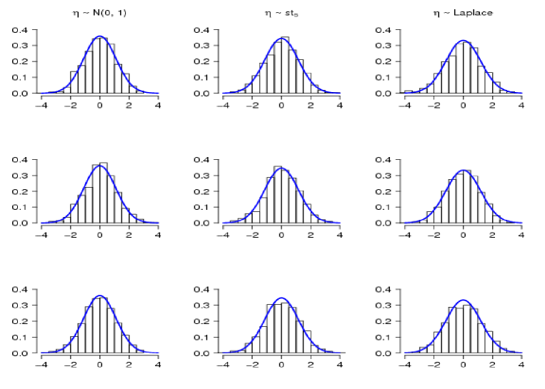
Table 2 shows the empirical mean (EM), empirical standard deviation (ESD), and asymptotic standard deviation (ASD) of the QMLE $\widehat{\theta}_{n}$ and the Lyapunov exponent estimator $\widehat{\gamma}_{n}$. The ASD of $\widehat{\gamma}_{n}$ and $\widehat{\theta}_{n}$ is calculated by the asymptotic covariance matrix in Theorems 3.1 and 4.1, respectively, where the theoretical values of $\sigma_{\gamma_{0}}^{2}$ are given in Table 1, and the theoretical values of $\kappa_{4}$ are 3, 9 and 6 for $N(0,1)$, $\mathrm{st}_{5}$, and Laplace distributions, respectively. From this table, we can see that the larger the sample size, the closer the EMs and their corresponding true values, and also the closer the ESDs and ASDs. Particularly, $\widehat{\gamma}_{n}$ performs well even though $\gamma_{0}$ is very small. To assess the overall performance of $\widehat{\gamma}_{n}$, Fig.2 plots the empirical density of $\sqrt{n}(\widehat{\gamma}_{n}-\gamma_{0})$ for different $\alpha_{0}$ in Table 1. From Fig.2, we find that $\widehat{\gamma}_{n}$ has a good performance in all cases.

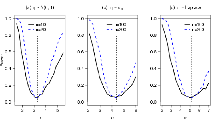
Next, we examine the performance of test statistic $T_{n}$ in (3.1) for testing the hypothesis $H_{0}:\gamma_{0}=0$ against $H_{1}:\gamma_{0}\neq 0$. Fig. 3 shows the power and size of $T_{n}$ for $n=100$ and 200 when $\alpha_{0}$ varies, and the size of $T_{n}$ corresponds to the case that $\alpha_{0}=3.3058$ (for $N(0,1)$), 4.3697 (for $\mathrm{st}_{5}$) and 5.1726 (for Laplace); see Table 1. From this figure, we can see that $T_{n}$ has a very precise size, and overall, the power to detect the instability is significant, even when sample size is small.

Figure 2: The histograms of $\sqrt{n}(\widehat{\gamma}_{n}-\gamma_{0})$ when $\eta$ is $N(0,1)$, $\mathrm{st}_{5}$, and Laplace distribution, respectively. The curves are the densities of $N(0,\sigma_{\gamma_{0}}^{2})$. Here the true parameter $\phi_{0}=0.5$ and the values of $\alpha_{0}$ and $\sigma_{\gamma_{0}}^{2}$ are given in Table 1, respectively. The top, middel, and bottom panels correspond to $\gamma_{0}<0$, $\gamma_{0}=0$, and $\gamma_{0}>0$, respectively. The sample size is 200.

Figure 3: The power and size of $T_{n}$ at the significance level 5% when $\eta$ is $N(0,1)$, $\mathrm{st}_{5}$ and Laplace distribution, respectively.

6 An empirical example

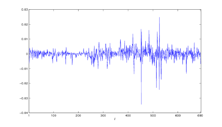
This section applies the DARWIN(1) model to study the daily exchange rates of New Taiwan Dollars (TWD) to United States Dollars (USD) from January 1, 2007 to December 31, 2009, which has in total 692 observations. The log-returns of this exchange rate series, denoted by $\{y_{t}\}_{t=1}^{691}$, are plotted in Fig.4.

Figure 4: The log-return of daily exchange rates of New Taiwan Dollars (TWD) to United States Dollars (USD) from January 1, 2007 to December 31, 2009.

First, we use model (1.2) with the QMLE estimation to fit $\{y_{t}\}$ by

$$y_{t}=0.3666_{(0.1661)}y_{t-1}+\eta_{t}\sqrt{19.0586_{(5.3083)}\,y_{t-1}^{2}},$$ (6.1)

where the values in parentheses are estimated standard errors. Based on the residuals $\{\widehat{\eta}_{t}\}$, Fig.5 plots the ACF and PACF of $\{\widehat{\eta}_{t}\}$ and $\{\widehat{\eta}_{t}^{2}\}$. From this figure, it seems that model (6.1) is adequate. Next, we use the Mira test and the Cabilio-Masaro test in R package lawstat to test the symmetry of $\eta_{t}$, and find that their p-values are 0.2985 and 0.2280, respectively. Therefore, we accept the hypothesis that $\eta_{t}$ is symmetric at the significance level 5%. Moreover, we use the Wald test statistic $W_{n}$ to detect the hypothesis $H_{0}:\phi_{0}=0$. The p-value of $W_{n}$ is 0.0273, and it turns out that we can reject $H_{0}$ at the significance level 5%. On the other hand, we find that the estimated Lyapunov exponent $\widehat{\gamma}_{n}=0.0001$ with $\widehat{\sigma}_{\gamma}^{2}=1.4651$, and this implies that the value of test statistic $T_{n}=0.0019$. Clearly, the null hypothesis of $\gamma_{0}=0$ is not rejected at the significance level 5%. Thus, there is no statistical evidence against the hypothesis that the return process is stable, i.e., log volatility of $y_{t}$ is a random walk.

Figure 5: The top (or bottom) panel is the ACF and PACF of $\{\widehat{\eta}_{t}\}$ (or $\{\widehat{\eta}_{t}^{2}\})$

Figure 6: The top (or bottom) panel is the ACF and PACF of $\{\widetilde{\eta}_{t}\}$ (or $\{\widetilde{\eta}_{t}^{2}\})$

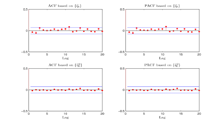
It is also interesting to apply model (1) to fit $\{y_{t}\}$. The fitted model with the QMLE estimation is

$$y_{t}=0.0317_{(0.0321)}y_{t-1}+\eta_{t}\sqrt{9.3\times 10^{-6}_{(0.1030)}+0.3349_{(0.0214)}y_{t-1}^{2}},$$ (6.2)

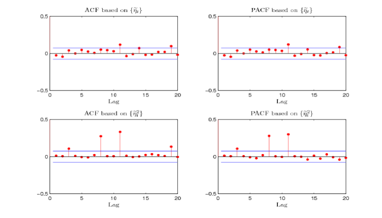
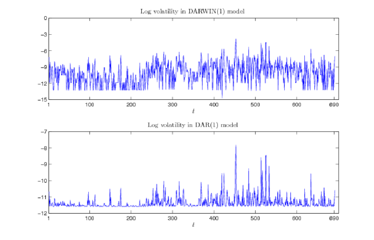
where the values in parentheses are estimated standard errors. Clearly, the estimate of $\omega_{0}$ is very close to zero. Let $\{\widetilde{\eta}_{t}\}$ be the residuals of model (6.2). Fig.6 plots the ACF and PACF of $\{\widetilde{\eta}_{t}\}$ and $\{\widetilde{\eta}_{t}^{2}\}$, suggesting that model (6.2) is not adequate. Based on these facts, it implies that model (6.1) is preferred to fit $\{y_{t}\}$. To gain more insight, we plot the estimated log volatilities of models (6.1) and (6.2) in Fig.7. The log volatility of model (6.2) is bounded from below by the logarithm of the intercept term, while there is no such bound in model (6.1). Among years 2007-2009, the financial crisis happened so that the log volatilities probably tend to have no lower bound, and hence this might lead to the preference of model (6.1) in fitting $\{y_{t}\}$.

Figure 7: The top (or bottom) is the log volatility in model (6.1) (or (6.2)).

7 Concluding remarks

This paper proposes a DARWIN(1) model. This new model is non-stationary and heteroskedastic, but unlike non-stationary DAR model, it includes a close-to-unit root type behavior of volatility in the stability case. In order to study the stability of the DARWIN(1) model, an easy-to-implement estimator of the Lyapunov exponent and a test for the stability have been constructed. Moreover, this paper studies the QMLE of the DARWIN(1) model, and finds that the asymptotic theory of the QMLE is invariant regardless of the stability of the model. An empirical example on TWD/USD exchange rates illustrates the importance of the DARWIN(1) model.

As one natural extension work, one can apply the principle of setting the intercept to zero to high-order DAR models or conditional heteroscedastic models, which would produce a branch of models that totally differ from the classical counterparts in the literature. Finally, it is worthy noting that how to test the DARWIN model in the null against the counterpart DAR model in the alternative is an interesting open question. The traditional tests, e.g., the likelihood ratio test, the Lagrange multiplier test and the Wald test, or their one-sided counterparts, may not work due to the nonstationarity of DARWIN models. How to develop powerful tests for such hypothesis would be a promising but challenging direction for future study.

Appendix: Technical Proofs

Proof of Theorem 3.1

By the definition of $\widehat{\gamma}_{n}$, we have

$$\widehat{\gamma}_{n}=\frac{1}{n}\sum_{t=1}^{n}\log\Big{(}\frac{|y_{t}|}{|y_{t-1}|}\Big{)}=\frac{1}{n}\sum_{t=1}^{n}\log\big{|}\phi_{0}+\eta_{t}\mathrm{sign}(y_{t-1})\sqrt{\alpha_{0}}\big{|}.$$

Since $(\eta_{1}\mathrm{sign}(y_{0}),...,\eta_{t}\mathrm{sign}(y_{t-1}))\stackrel{{\scriptstyle d}}{{=}}(\eta_{1},...,\eta_{t})$ by the induction over $t\geq 1$, we have

$$\widehat{\gamma}_{n}\stackrel{{\scriptstyle d}}{{=}}\frac{1}{n}\sum_{t=1}^{n}\log\big{|}\phi_{0}+\eta_{t}\sqrt{\alpha_{0}}\big{|}.$$

Thus, the result holds.

Proof of Theorem 4.1

A simple calculation yields that

$$\widehat{\phi}_{n}=\phi_{0}+\frac{\sqrt{\alpha_{0}}}{n}\sum_{t=1}^{n}\eta_{t}\mathrm{sign}(y_{t-1})\quad\mbox{and}\quad\widehat{\alpha}_{n}=\frac{\alpha_{0}}{n}\sum_{t=1}^{n}\eta_{t}^{2}-(\widehat{\phi}_{n}-\phi_{0})^{2}.$$

Note that $\{\eta_{t}\mathrm{sign}(y_{t-1})\}$ is a martingale difference with respect to $\mathcal{F}_{t}=\sigma(\eta_{i},i\leq t)$. Thus, $\widehat{\phi}_{n}$ is unbiased. Also, $E(\widehat{\alpha}_{n})=\frac{n-1}{n}\alpha_{0}$. Thus, (i) holds.

By Theorem 2.19 in Hall and Hedye (1980), we have $\frac{1}{n}\sum_{t=1}^{n}\eta_{t}\mathrm{sign}(y_{t-1})\rightarrow 0$ a.s., which implies that $\widehat{\phi}_{n}\rightarrow\phi_{0}$ a.s., and then $\widehat{\alpha}_{n}\rightarrow\alpha_{0}$ a.s. by the strong law of large numbers. Thus, (ii) holds.

For (iii), note that

$$\sqrt{n}(\widehat{\phi}_{n}-\phi_{0}) =\frac{\sqrt{\alpha_{0}}}{\sqrt{n}}\sum_{t=1}^{n}\eta_{t}\mathrm{sign}(y_{t-1})\,,$$

$$\sqrt{n}(\widehat{\alpha}_{n}-\alpha_{0}) =\frac{\alpha_{0}}{\sqrt{n}}\sum_{t=1}^{n}(\eta_{t}^{2}-1)-\frac{1}{\sqrt{n}}\left(\sqrt{n}(\widehat{\phi}_{n}-\phi_{0})\right)^{2}.$$

By the Cramér-Wold device and the martingale central limit theorem in Brown (1971), the proof of (iii) is trivial.

REFERENCES

Billingsley, P. (1999). Convergence of Probability Measures(2nd). Wiley.

Borkovec, M. (2000). Extremal behavior of the autoregressive process with ARCH(1) errors. Stochastic Process. Appl. 85, 189–207.

Brown, B. M. (1971). Martingale central limit theorems. Ann. Math. Statist. 42, 59–66.

Borkovec, M. and Klüppelberg, C. (2001). The tail of the stationary distribution of an autoregressive process with ARCH(1) errors. Ann. Appl. Prob. 11, 1220–1241.

Bollerslev, T, Chou, R.Y. and Kroner, K.F. (1992). ARCH modeling in finance: A review of the theory and empirical evidence. J. Econometrics 52, 5–59.

Chan, N. H. and Peng, L. (2005). Weighted least absolute deviation estimation for an AR(1) process with ARCH(1) errors. Biometrika 92, 477–484.

Chen, M., Li, D. and Ling, S. (2014). Non-stationarity and quasi-maximum likelihood estimation on a double autoregressive model. J. Time Series Anal. 35, 189-202.

Cline, D. B. H and Pu, H. H. (2004). Stability and the Lyapounov exponent of threshold AR-ARCH models. Ann. Appl. Prob. 14, 1920–1949.

Engle, R.F. (1982). Autoregressive conditional heteroscedasticity with estimates of the variance of United Kingdom inflation. Econometrica 50, 987–1007.

Francq, C. and Zakoïan, J.-M. (2010). GARCH Models: Structure, Statistical Inference and Financial Applications. John Wiley.

Francq, C. and Zakoïan, J.-M. (2012). Strict stationarity testing and estimation of explosive and stationary generalized autoregressive conditional heteroscedasticity models. Econometrica 80, 821–861.

Guégan, D. and Diebolt, J. (1994). Probabilistic properties of the $\beta$-ARCH-model. Statist. Sinica 4, 71–87.

Guo, S., Ling, S. and Zhu, K. (2014). Factor double autoregressive models with application to simultaneous causality testing. J. Statist. Plann. Inference 148, 82–94.

Hafner, C. M. and Preminger, A. (2015). An ARCH model without intercept. Econom. Lett. 129, 13–17.

Hall, P. and Heyde, C. C. (1980). Martingale limit theory and its application. Academic Press, New York.

Li, D., Guo, S. and Li, M. (2015). Robust inference in a double AR model. Working paper.

Li, D., Li, M. and Wu, W. (2014). On dynamics of volatilities in nonstationary GARCH models. Statist. Probab. Lett. 94, 86–90.

Li, D., Ling, S. and Zakoïan, J.-M. (2015). Asymptotic inference in multiple-threshold double autoregressive models. Forthcoming in J. Econometrics.

Li, D., Ling, S. and Zhang, R.M. (2015). On a threshold double autoregressive model. Forthcoming in J. Bus. Econom. Statist.

Ling, S. (2004). Estimation and testing stationarity for double autoregressive models. J. Roy. Statist. Soc. Ser. B 66, 63–78.

Ling, S. (2007). A double AR(p) model: structure and estimation. Statist. Sinica 17, 161–175.

Ling, S. and Li, D. (2008). Asymptotic inference for a nonstationary double AR(1) model. Biometrika 95, 257–263.

Ling, S., Zhu, K. and Chong, C.Y. (2013). Diagnostic checking for non-stationary ARMA models with an application to financial data. North American Journal of Economics and Finance 26, 624–639.

Ljung, G. M. and Box, G. E. P. (1978). On a measure of lack of fit in time series models. Biometrika 65, 297–303.

Lu, Z. (1998). On the geometric ergodicity of a non-linear autoregressive model with an autoregressive conditional heteroscedastic term. Statist. Sinica 8, 1205–1217.

McLeod, A. I. and Li, W. K. (1983). Disgnostic checking ARMA times series models using squared-residual autocorrelations. J. Time Ser. Anal. 4, 269–273.

Weiss, A. A. (1984). ARMA models with ARCH errors. J. Time Ser. Anal. 5, 129–143.

Zhu, K. and Ling, S. (2013). Quasi-maximum exponential likelihood estimators for a double AR($p$) model. Statist. Sinica 23, 251–270.