Abstract

In this paper we make a further step towards a dispersive description of the hadronic light-by-light (HLbL) tensor, which should ultimately lead to a data-driven evaluation of its contribution to $(g-2)_{\mu}$. We first provide a Lorentz decomposition of the HLbL tensor performed according to the general recipe by Bardeen, Tung, and Tarrach, generalizing and extending our previous approach, which was constructed in terms of a basis of helicity amplitudes. Such a tensor decomposition has several advantages: the role of gauge invariance and crossing symmetry becomes fully transparent; the scalar coefficient functions are free of kinematic singularities and zeros, and thus fulfill a Mandelstam double-dispersive representation; and the explicit relation for the HLbL contribution to $(g-2)_{\mu}$ in terms of the coefficient functions simplifies substantially. We demonstrate explicitly that the dispersive approach defines both the pion-pole and the pion-loop contribution unambiguously and in a model-independent way. The pion loop, dispersively defined as pion-box topology, is proven to coincide exactly with the one-loop scalar QED amplitude, multiplied by the appropriate pion vector form factors.

0cm 4(-6,2) INT-PUB-15-019
UWTHPH-2015-10

 

1 Introduction

The anomalous magnetic moment of the muon, $a_{\mu}=(g-2)_{\mu}/2$, is one of the very rare quantities in particle physics where a significant discrepancy between its experimental determination and the Standard-Model evaluation still persists. A robust, reliable estimate of the theoretical uncertainties is thus mandatory, especially in view of the projected accuracy of the forthcoming $(g-2)_{\mu}$ experiments at FNAL [1] and J-PARC [2], to settle whether this discrepancy can be attributed to New Physics.

The uncertainty on the theory side is dominated by hadronic contributions, see e.g. [3, 4, 5], the largest error arising from hadronic vacuum polarization (HVP). Since HVP is straightforwardly related to the total $e^{+}e^{-}$ hadronic cross section via a dispersion relation, the evaluation of this contribution is expected to become more accurate within the next few years [6] thanks to upcoming improvements in the experimental input, although reducing further the present sub-percent accuracy will be challenging. This implies that hadronic light-by-light (HLbL) scattering is likely to soon dominate the theory uncertainty in $a_{\mu}$. Using previous approaches [11, 12, 13, 14, 15, 16, 17, 18, 19, 20, 21, 22], systematic errors are difficult, if not impossible, to quantify. A novel strategy is required to go beyond the state of the art, to avoid or at least reduce model dependence to a minimum, make a solid estimate of theoretical errors, and possibly reduce them. Lattice QCD is a natural candidate to achieve this goal, but it is not clear yet if or when this method will become competitive [23, 24, 25]. Alternatively, as we recently argued [26], it is possible to establish a rigorous framework based on dispersion theory that directly links $a_{\mu}^{\rm HLbL}$ to experimentally accessible on-shell form factors and scattering amplitudes [27], contrary to what has been previously conjectured [28, 12, 24, 29].

Our dispersive formalism is based on the fundamental principles of unitarity, analyticity, crossing symmetry, and gauge invariance. The derivation of such a systematic framework becomes challenging due to the fact that HLbL scattering is described by a hadronic four-point function whose properties are significantly more complicated than those of the two-point function entering HVP. Besides the opportunity to achieve a data-driven evaluation of $a_{\mu}^{\rm HLbL}$, this approach allows us to unambiguously define and evaluate the various low-energy contributions to HLbL scattering, most notably pion pole and pion loop.

The key result of [26] was a master formula giving the contribution to $a_{\mu}^{\rm HLbL}$ from the pion-pole term and intermediate $\pi\pi$ states expressed in terms of the pion transition form factor and helicity partial waves for $\gamma^{*}\gamma^{*}\to\pi\pi$. In the present paper we reformulate this approach in a more general context, by employing a different generating set for the Lorentz structures of the HLbL tensor. This new set, which we constructed following the prescription by Bardeen, Tung [31], and Tarrach [32] (BTT), has the property of being explicitly free of kinematic singularities and zeros [33]. Therefore, the scalar coefficient functions associated with each Lorentz structure of this generating set are also free of kinematic singularities and zeros, and thus fulfill a Mandelstam double-dispersive representation. Further motivation for deriving such a BTT set is provided by the fact that the role of gauge invariance and crossing symmetry becomes fully transparent, with constraints from soft-photon zeros incorporated automatically. Moreover, the absence of kinematic singularities makes it much easier to perform the angular averages necessary to calculate the contribution to $(g-2)_{\mu}$ — indeed both the derivation and the final form of the master formula are simplified considerably in the present setting, and allow for a simpler inclusion of partial-wave contributions beyond $S$-waves. In the derivation of the master formula it is very useful to perform a Wick rotation of the integration variables. This has been already used in several papers in the literature without ever addressing an important subtlety which is relevant in the present case: namely if the Wick rotation goes through without changes even if the integrand is a loop function showing anomalous thresholds. We discuss this point in detail and prove that this is indeed the case. Finally, the BTT formulation facilitates the proof that both pion-pole and pion-loop contributions are uniquely defined in the dispersive approach, and confirms the relation to the pion transition form factor and the pion electromagnetic form factor given in [26]. We explicitly proof that the scalar QED (sQED) pion loop dressed with pion form factors (denoted by FsQED in [26]) is identical to the contribution from $\pi\pi$ intermediate states with a pion-pole left-hand cut (LHC).

In summary, this paper contains three main results: (i) the explicit construction of the BTT decomposition of the HLbL tensor; (ii) the derivation of the master formula expressing the HLbL contribution in terms of the BTT scalar functions; (iii) the proof that in the dispersive approach the FsQED contribution is uniquely defined. Everything which goes beyond the FsQED contribution is amenable to partial-wave expansion and will be discussed in full detail in a forthcoming publication.

The present paper is structured as follows. In Sect. 2, we first review some aspects of the process $\gamma^{*}\gamma^{*}\to\pi\pi$, mainly as an illustration of the techniques that we apply afterwards to HLbL. In Sect. 3, we derive the decomposition of the HLbL tensor into a set of scalar functions that are free of kinematics. In Sect. 4, this BTT decomposition is then used to derive a master formula for $a_{\mu}^{\rm HLbL}$ that is parametrized by the corresponding scalar functions. We verify the validity of the Wick rotation of the two-loop integral in the calculation of $a_{\mu}^{\rm HLbL}$, even in the case of anomalous thresholds in the HLbL tensor. In Sect. 5, we derive a Mandelstam representation of the BTT scalar functions, and, by comparison to the loop formulation of the sQED pion loop, demonstrate that it indeed coincides with the contribution of $\pi\pi$ intermediate states with a pion-pole LHC. We conclude with an outlook in Sect. 6, while some of the lengthier expressions and derivations are collected in the appendices.

2 The sub-process $\boldsymbol{\gamma^{*}\gamma^{*}\to\pi\pi}$

As a prelude, we discuss in this section the process $\gamma^{*}\gamma^{*}\to\pi\pi$, which will become important as a sub-process when we write down a dispersion relation for the HLbL tensor. Because the Lorentz structure of $\gamma^{*}\gamma^{*}\to\pi\pi$ is much simpler than the one of light-by-light scattering, it also allows us to illustrate a technique for the construction of amplitudes that are free of kinematic singularities and zeros, which we will apply afterwards to the more complicated case of HLbL. In order to render this analogy manifest, we slightly change conventions compared to [26]: we identify here $\gamma^{*}\gamma^{*}\to\pi\pi$ as the $s$-channel process instead of $\gamma^{*}\pi\to\gamma^{*}\pi$. This assignment is slightly unnatural when it comes to constructing dispersion relations for a process with these crossing properties, see [34, 35, 36, 37], but makes the inclusion into the unitarity relation in HLbL more straightforward.

2.1 Kinematics and matrix element

Figure 1: $\gamma^{*}\gamma^{*}\to\pi\pi$ as a sub-process of $e^{+}e^{-}\to e^{+}e^{-}\pi\pi$.

Consider the process

$$e^{+}(k_{1})e^{-}(k_{2})\to e^{+}(k_{3})e^{-}(k_{4})\gamma^{*}(q_{1})\gamma^{*}(q_{2})\to e^{+}(k_{3})e^{-}(k_{4})\pi^{a}(p_{1})\pi^{b}(p_{2}),$$ (2.1)

shown in Fig. 1. At $\mathcal{O}(e^{4})$, the amplitude for this process is given by

$$\begin{split}i\mathcal{T}&=\bar{v}(k_{1})(-ie\gamma_{\alpha})v(k_{3})\bar{u}(k_{4})(-ie\gamma_{\beta})u(k_{2})\\ &\quad\times\frac{-i}{q_{1}^{2}}\left(g^{\alpha\mu}-(1-\xi)\frac{q_{1}^{\alpha}q_{1}^{\mu}}{q_{1}^{2}}\right)\frac{-i}{q_{2}^{2}}\left(g^{\beta\nu}-(1-\xi)\frac{q_{2}^{\beta}q_{2}^{\nu}}{q_{2}^{2}}\right)ie^{2}W_{\mu\nu}^{ab}(p_{1},p_{2},q_{1}),\end{split}$$ (2.2)

where $\xi$ is an arbitrary gauge parameter for the photon propagators and the tensor $W_{\mu\nu}^{ab}$ is defined as the pure QCD matrix element

$$W^{\mu\nu}_{ab}(p_{1},p_{2},q_{1})=i\int d^{4}x\,e^{-iq_{1}\cdot x}\langle\pi^{a}(p_{1})\pi^{b}(p_{2})|T\{j_{\mathrm{em}}^{\mu}(x)j_{\mathrm{em}}^{\nu}(0)\}|0\rangle.$$ (2.3)

The contraction thereof with appropriate polarization vectors may be understood as an amplitude for the off-shell process

$$\gamma^{*}(q_{1},\lambda_{1})\gamma^{*}(q_{2},\lambda_{2})\to\pi^{a}(p_{1})\pi^{b}(p_{2}),$$ (2.4)

where $\lambda_{1,2}$ denote the helicities of the off-shell photons. We define the connected part of such a matrix element by

$$\begin{split}\langle\pi^{a}(p_{1})&\pi^{b}(p_{2})|\gamma^{*}(q_{1},\lambda_{1})\gamma^{*}(q_{2},\lambda_{2})\rangle\\ :=&{}-e^{2}\epsilon_{\mu}^{\lambda_{1}}(q_{1})\epsilon_{\nu}^{\lambda_{2}}(q_{2})\int d^{4}x\,d^{4}y\,e^{-i(q_{1}\cdot x+q_{2}\cdot y)}\langle\pi^{a}(p_{1})\pi^{b}(p_{2})|T\{j_{\mathrm{em}}^{\mu}(x)j_{\mathrm{em}}^{\nu}(y)\}|0\rangle\\ =&{}-e^{2}(2\pi)^{4}\delta^{(4)}(p_{1}+p_{2}-q_{1}-q_{2})\epsilon_{\mu}^{\lambda_{1}}(q_{1})\epsilon_{\nu}^{\lambda_{2}}(q_{2})\\ &\quad\times\int d^{4}x\,e^{-iq_{1}\cdot x}\langle\pi^{a}(p_{1})\pi^{b}(p_{2})|T\{j_{\mathrm{em}}^{\mu}(x)j_{\mathrm{em}}^{\nu}(0)\}|0\rangle\\ =&{}ie^{2}(2\pi)^{4}\delta^{(4)}(p_{1}+p_{2}-q_{1}-q_{2})\epsilon_{\mu}^{\lambda_{1}}(q_{1})\epsilon_{\nu}^{\lambda_{2}}(q_{2})W^{\mu\nu}_{ab}(p_{1},p_{2},q_{1}).\end{split}$$ (2.5)

The helicity amplitudes are given by the contraction with polarization vectors:

$$\epsilon_{\mu}^{\lambda_{1}}(q_{1})\epsilon_{\nu}^{\lambda_{2}}(q_{2})W^{\mu\nu}_{ab}(p_{1},p_{2},q_{1})=e^{i(\lambda_{1}-\lambda_{2})\phi}H_{\lambda_{1}\lambda_{2}}^{ab}.$$ (2.6)

We introduce the following kinematic variables:

$$\begin{split}s&:=(q_{1}+q_{2})^{2}=(p_{1}+p_{2})^{2},\\ t&:=(q_{1}-p_{1})^{2}=(q_{2}-p_{2})^{2},\\ u&:=(q_{1}-p_{2})^{2}=(q_{2}-p_{1})^{2},\end{split}$$ (2.7)

which satisfy $s+t+u=q_{1}^{2}+q_{2}^{2}+2M_{\pi}^{2}$.

2.2 Tensor decomposition

The tensor $W^{\mu\nu}_{ab}$ can be decomposed based on Lorentz covariance as (we drop isospin indices)

$$W^{\mu\nu}=g^{\mu\nu}W_{1}+q_{i}^{\mu}q_{j}^{\nu}W_{2}^{ij},$$ (2.8)

where we abbreviate $q_{i}=\{q_{1},q_{2},p_{2}-p_{1}\}$ and where double indices are summed. The ten coefficient functions $\{W_{1},W_{2}^{ij}\}$ cannot contain any kinematic but only dynamic singularities. However, they have to fulfill kinematic constraints that are required e.g. by gauge invariance, hence they contain kinematic zeros. Conservation of the electromagnetic current implies the Ward identities

$$q_{1}^{\mu}W_{\mu\nu}=q_{2}^{\nu}W_{\mu\nu}=0,$$ (2.9)

hence a priori six relations between the scalar functions $\{W_{1},W_{2}^{ij}\}$. Only five of them are linearly independent and thus reduce the set of scalar functions to five independent ones.

We now construct a set of scalar functions which are free of both kinematic singularities and zeros. We follow the recipe given by Bardeen, Tung [31], and Tarrach [32]. As was shown in [32], the basis (consisting of five functions) constructed according to the recipe of [31] is not free of kinematic singularities. However, a redundant set of six structures can be constructed, which fulfills the requirement.

In the case of $\gamma^{*}\gamma^{*}\to\pi\pi$, there exists in addition to gauge invariance and crossing symmetry of the photons also the crossing (Bose) symmetry of the pions, which is responsible for additional kinematic zeros. In fact, this can be used to circumvent the introduction of a sixth function, reducing the set again to five scalar functions free of both kinematic singularities and zeros. This was first derived in [38] in the context of doubly-virtual nucleon Compton scattering.

We define the projector

$$I^{\mu\nu}=g^{\mu\nu}-\frac{q_{2}^{\mu}q_{1}^{\nu}}{q_{1}\cdot q_{2}},$$ (2.10)

which satisfies

$$\begin{split}q_{1}^{\mu}I_{\mu\nu}&=q_{2}^{\nu}I_{\mu\nu}=0,\\ {I_{\mu}}^{\lambda}W_{\lambda\nu}&=W_{\mu\lambda}{I^{\lambda}}_{\nu}=W_{\mu\nu},\end{split}$$ (2.11)

i.e. the tensor $W^{\mu\nu}$ is invariant under contraction with the projector, but contracting the projector with any Lorentz structure produces a gauge-invariant structure.

We apply this projector for both photons:

$$W_{\mu\nu} =I_{\mu\mu^{\prime}}I_{\nu^{\prime}\nu}W^{\mu^{\prime}\nu^{\prime}}=\sum_{i=1}^{5}\bar{T}_{\mu\nu}^{i}\bar{B}_{i},$$ (2.12)

where

$$\bar{T}_{1}^{\mu\nu} =g^{\mu\nu}-\frac{q_{2}^{\mu}q_{1}^{\nu}}{q_{1}\cdot q_{2}}, \bar{B}_{1} =W_{1},$$

$$\bar{T}_{2}^{\mu\nu} =q_{1}^{\mu}q_{2}^{\nu}-\frac{q_{1}^{2}q_{2}^{\mu}q_{2}^{\nu}}{q_{1}\cdot q_{2}}-\frac{q_{2}^{2}q_{1}^{\mu}q_{1}^{\nu}}{q_{1}\cdot q_{2}}+\frac{q_{1}^{2}q_{2}^{2}q_{2}^{\mu}q_{1}^{\nu}}{(q_{1}\cdot q_{2})^{2}}, \bar{B}_{2} =W_{2}^{12},$$

$$\bar{T}_{3}^{\mu\nu} =q_{1}^{\mu}q_{3}^{\nu}-\frac{q_{1}^{2}q_{2}^{\mu}q_{3}^{\nu}}{q_{1}\cdot q_{2}}-\frac{q_{2}\cdot q_{3}q_{1}^{\mu}q_{1}^{\nu}}{q_{1}\cdot q_{2}}+\frac{q_{1}^{2}q_{2}\cdot q_{3}q_{2}^{\mu}q_{1}^{\nu}}{(q_{1}\cdot q_{2})^{2}}, \bar{B}_{3} =W_{2}^{13},$$

$$\bar{T}_{4}^{\mu\nu} =q_{3}^{\mu}q_{2}^{\nu}-\frac{q_{2}^{2}q_{3}^{\mu}q_{1}^{\nu}}{q_{1}\cdot q_{2}}-\frac{q_{1}\cdot q_{3}q_{2}^{\mu}q_{2}^{\nu}}{q_{1}\cdot q_{2}}+\frac{q_{2}^{2}q_{1}\cdot q_{3}q_{2}^{\mu}q_{1}^{\nu}}{(q_{1}\cdot q_{2})^{2}}, \bar{B}_{4} =W_{2}^{32},$$

$$\bar{T}_{5}^{\mu\nu} =q_{3}^{\mu}q_{3}^{\nu}-\frac{q_{1}\cdot q_{3}q_{2}^{\mu}q_{3}^{\nu}}{q_{1}\cdot q_{2}}-\frac{q_{2}\cdot q_{3}q_{3}^{\mu}q_{1}^{\nu}}{q_{1}\cdot q_{2}}+\frac{q_{1}\cdot q_{3}q_{2}\cdot q_{3}q_{2}^{\mu}q_{1}^{\nu}}{(q_{1}\cdot q_{2})^{2}}, \bar{B}_{5} =W_{2}^{33}.$$

As the functions $\bar{B}_{i}$ are a subset of the original scalar functions, they are still free of kinematic singularities, but contain zeros, because the Lorentz structures contain singularities. We have to remove now the single and double poles in $q_{1}\cdot q_{2}$ from the Lorentz structures $\bar{T}_{i}^{\mu\nu}$. This is achieved as follows [31]:

• remove as many double poles as possible by adding to the structures linear combinations of other structures with non-singular coefficients,

• if no more double poles can be removed in this way, multiply the structures that still contain double poles by $q_{1}\cdot q_{2}$,

• proceed in the same way with single poles.

It turns out that no double poles in $q_{1}\cdot q_{2}$ can be removed by adding to the structures multiples of the other structures, hence $\bar{T}_{2}^{\mu\nu}$, …, $\bar{T}_{5}^{\mu\nu}$ have to be multiplied by $q_{1}\cdot q_{2}$. The resulting simple poles can be removed by adding multiples of $\bar{T}_{1}^{\mu\nu}$. In the end, we have to multiply $\bar{T}_{1}^{\mu\nu}$ by $q_{1}\cdot q_{2}$ in order to remove the last pole. We then arrive at the following representation:

$$W_{\mu\nu} =\sum_{i=1}^{5}\tilde{T}_{\mu\nu}^{i}\tilde{B}_{i},$$ (2.14)

where

$$\begin{split}\tilde{T}_{1}^{\mu\nu}&=q_{1}\cdot q_{2}g^{\mu\nu}-q_{2}^{\mu}q_{1}^{\nu},\\ \tilde{T}_{2}^{\mu\nu}&=q_{1}^{2}q_{2}^{2}g^{\mu\nu}+q_{1}\cdot q_{2}q_{1}^{\mu}q_{2}^{\nu}-q_{1}^{2}q_{2}^{\mu}q_{2}^{\nu}-q_{2}^{2}q_{1}^{\mu}q_{1}^{\nu},\\ \tilde{T}_{3}^{\mu\nu}&=q_{1}^{2}q_{2}\cdot q_{3}g^{\mu\nu}+q_{1}\cdot q_{2}q_{1}^{\mu}q_{3}^{\nu}-q_{1}^{2}q_{2}^{\mu}q_{3}^{\nu}-q_{2}\cdot q_{3}q_{1}^{\mu}q_{1}^{\nu},\\ \tilde{T}_{4}^{\mu\nu}&=q_{2}^{2}q_{1}\cdot q_{3}g^{\mu\nu}+q_{1}\cdot q_{2}q_{3}^{\mu}q_{2}^{\nu}-q_{2}^{2}q_{3}^{\mu}q_{1}^{\nu}-q_{1}\cdot q_{3}q_{2}^{\mu}q_{2}^{\nu},\\ \tilde{T}_{5}^{\mu\nu}&=q_{1}\cdot q_{3}q_{2}\cdot q_{3}g^{\mu\nu}+q_{1}\cdot q_{2}q_{3}^{\mu}q_{3}^{\nu}-q_{1}\cdot q_{3}q_{2}^{\mu}q_{3}^{\nu}-q_{2}\cdot q_{3}q_{3}^{\mu}q_{1}^{\nu},\end{split}$$ (2.15)

and

$$\tilde{B}_{1} =\frac{1}{q_{1}\cdot q_{2}}W_{1}-\frac{q_{1}^{2}q_{2}^{2}}{(q_{1}\cdot q_{2})^{2}}W_{2}^{12}-\frac{q_{1}^{2}q_{2}\cdot q_{3}}{(q_{1}\cdot q_{2})^{2}}W_{2}^{13}-\frac{q_{2}^{2}q_{1}\cdot q_{3}}{(q_{1}\cdot q_{2})^{2}}W_{2}^{32}-\frac{q_{1}\cdot q_{3}q_{2}\cdot q_{3}}{(q_{1}\cdot q_{2})^{2}}W_{2}^{33},$$

$$\tilde{B}_{2} =\frac{1}{q_{1}\cdot q_{2}}W_{2}^{12},$$

$$\tilde{B}_{3} =\frac{1}{q_{1}\cdot q_{2}}W_{2}^{13},$$

$$\tilde{B}_{4} =\frac{1}{q_{1}\cdot q_{2}}W_{2}^{32},$$

$$\tilde{B}_{5} =\frac{1}{q_{1}\cdot q_{2}}W_{2}^{33}.$$

The Lorentz structures (2.15) agree with the basis used in [26], upon $q_{2}\to-q_{2}$, $p_{1}\to-p_{1}$ due to crossing and the identification

$$\tilde{T}_{1,\mu\nu}=T_{1,\mu\nu}^{\text{\cite[cite]{[\@@bibref{Number}{Colangelo2014a}{}{}]}}},\qquad\tilde{T}_{2,\mu\nu}=T_{3,\mu\nu}^{\text{\cite[cite]{[\@@bibref{Number}{Colangelo2014a}{}{}]}}},\qquad\tilde{T}_{3,\mu\nu}=\frac{1}{2}T_{4,\mu\nu}^{\text{\cite[cite]{[\@@bibref{Number}{Colangelo2014a}{}{}]}}},\qquad\tilde{T}_{4,\mu\nu}=-\frac{1}{2}T_{5,\mu\nu}^{\text{\cite[cite]{[\@@bibref{Number}{Colangelo2014a}{}{}]}}},\qquad\tilde{T}_{5,\mu\nu}=\frac{1}{4}T_{2,\mu\nu}^{\text{\cite[cite]{[\@@bibref{Number}{Colangelo2014a}{}{}]}}}.$$ (2.17)

As shown by Tarrach, this basis is not free of kinematic singularities and zeros [32]. The structures $\tilde{T}_{i}^{\mu\nu}$ form a basis for $q_{1}\cdot q_{2}\neq 0$, but are degenerate for $q_{1}\cdot q_{2}=0$. This degeneracy implies that there is a linear combination of the structures $\tilde{T}_{i}^{\mu\nu}$ that is proportional to $q_{1}\cdot q_{2}$:

$$q_{1}\cdot q_{3}q_{2}\cdot q_{3}\tilde{T}_{2}^{\mu\nu}-q_{2}^{2}q_{1}\cdot q_{3}\tilde{T}_{3}^{\mu\nu}-q_{1}^{2}q_{2}\cdot q_{3}\tilde{T}_{4}^{\mu\nu}+q_{1}^{2}q_{2}^{2}\tilde{T}_{5}^{\mu\nu}=q_{1}\cdot q_{2}\tilde{T}_{6}^{\mu\nu},$$ (2.18)

where

$$\tilde{T}_{6}^{\mu\nu}=\left(q_{1}^{2}q_{3}^{\mu}-q_{1}\cdot q_{3}q_{1}^{\mu}\right)\left(q_{2}^{2}q_{3}^{\nu}-q_{2}\cdot q_{3}q_{2}^{\nu}\right).$$ (2.19)

Hence, in order to have a generating set even at $q_{1}\cdot q_{2}=0$ this sixth structure $\tilde{T}_{6}^{\mu\nu}$ has to be added by hand. Projected on the basis, it gives coefficients with poles in $q_{1}\cdot q_{2}$. Although the basis is not free of kinematic singularities and zeros, we have found the exact form of the singularities:

$$W_{\mu\nu} =\sum_{i=1}^{5}\tilde{T}_{\mu\nu}^{i}\tilde{B}_{i}=\sum_{i=1}^{6}\tilde{T}_{\mu\nu}^{i}B_{i},$$ (2.20)

where

$$\begin{split}\tilde{B}_{1}&=B_{1},\\ \tilde{B}_{2}&=B_{2}+\frac{q_{1}\cdot q_{3}q_{2}\cdot q_{3}}{q_{1}\cdot q_{2}}B_{6},\\ \tilde{B}_{3}&=B_{3}-\frac{q_{2}^{2}q_{1}\cdot q_{3}}{q_{1}\cdot q_{2}}B_{6},\\ \tilde{B}_{4}&=B_{4}-\frac{q_{1}^{2}q_{2}\cdot q_{3}}{q_{1}\cdot q_{2}}B_{6},\\ \tilde{B}_{5}&=B_{5}+\frac{q_{1}^{2}q_{2}^{2}}{q_{1}\cdot q_{2}}B_{6}.\end{split}$$ (2.21)

The functions $B_{i}$ are free of kinematic singularities. The tensor structures can be written in terms of the Mandelstam variables $t$ and $u$ as

$$\begin{split}\tilde{T}_{1}^{\mu\nu}&=q_{1}\cdot q_{2}g^{\mu\nu}-q_{2}^{\mu}q_{1}^{\nu},\\ \tilde{T}_{2}^{\mu\nu}&=q_{1}^{2}q_{2}^{2}g^{\mu\nu}+q_{1}\cdot q_{2}q_{1}^{\mu}q_{2}^{\nu}-q_{1}^{2}q_{2}^{\mu}q_{2}^{\nu}-q_{2}^{2}q_{1}^{\mu}q_{1}^{\nu},\\ \tilde{T}_{3}^{\mu\nu}&=q_{1}\cdot q_{2}q_{1}^{\mu}q_{3}^{\nu}-q_{1}^{2}q_{2}^{\mu}q_{3}^{\nu}-\frac{1}{2}(t-u)q_{1}^{2}g^{\mu\nu}+\frac{1}{2}(t-u)q_{1}^{\mu}q_{1}^{\nu},\\ \tilde{T}_{4}^{\mu\nu}&=q_{1}\cdot q_{2}q_{3}^{\mu}q_{2}^{\nu}-q_{2}^{2}q_{3}^{\mu}q_{1}^{\nu}+\frac{1}{2}(t-u)q_{2}^{2}g^{\mu\nu}-\frac{1}{2}(t-u)q_{2}^{\mu}q_{2}^{\nu},\\ \tilde{T}_{5}^{\mu\nu}&=q_{1}\cdot q_{2}q_{3}^{\mu}q_{3}^{\nu}-\frac{1}{4}(t-u)^{2}g^{\mu\nu}+\frac{1}{2}(t-u)\left(q_{3}^{\mu}q_{1}^{\nu}-q_{2}^{\mu}q_{3}^{\nu}\right),\\ \tilde{T}_{6}^{\mu\nu}&=q_{1}^{2}q_{2}^{2}q_{3}^{\mu}q_{3}^{\nu}+\frac{1}{2}(t-u)\left(q_{1}^{2}q_{3}^{\mu}q_{2}^{\nu}-q_{2}^{2}q_{1}^{\mu}q_{3}^{\nu}\right)-\frac{1}{4}(t-u)^{2}q_{1}^{\mu}q_{2}^{\nu}.\end{split}$$ (2.22)

The derivation of the Lorentz decomposition for $\gamma^{*}\gamma^{*}\to\pi\pi$ up to this point should illustrate the techniques that will be applied to the much more complicated case of HLbL in Sect. 3. In the case of $\gamma^{*}\gamma^{*}\to\pi\pi$, there is in fact a solution to get rid of the additional redundant structure without introducing kinematic singularities [38]. The necessary steps are discussed in the next subsection. Note that it is an open question whether an analogous procedure to get rid of all redundancies in HLbL exists, see the discussion below (3.29).

2.3 Kinematic zeros due to crossing antisymmetry

We have now constructed a redundant set of six Lorentz structures. All kinematic constraints from gauge invariance are implemented and the scalar coefficient functions $B_{i}$ are free of kinematic singularities. However, due to the crossing symmetry of the pions, additional kinematic zeros are present in the functions $B_{i}$. As noted in [38], this can be exploited to eliminate the redundancy and to work again with basis coefficient functions free of kinematic singularities and zeros.

Since the two-photon state is even under charge conjugation, so must be the two-pion state. Therefore, the isospin $I=1$ amplitude vanishes. Bose symmetry implies that the amplitude and hence the tensor $W^{\mu\nu}$ is invariant under $p_{1}\leftrightarrow p_{2}$ or equivalently $q_{3}\leftrightarrow-q_{3}$. Under this transformation, the tensor structures $\tilde{T}_{i}^{\mu\nu}$ are even for $i=1,2,5,6$ and odd for $i=3,4$. Hence, $B_{1,2,5,6}$ are even, while $B_{3,4}$ must be odd. They contain a kinematic zero of the form

$$B_{3,4}=(t-u)\hat{B}_{3,4},$$ (2.23)

where $\hat{B}_{3,4}$ are free of kinematic singularities.

Crossing symmetry of the photons requires the invariance of $W^{\mu\nu}$ under $q_{1}\leftrightarrow q_{2}$, $\mu\leftrightarrow\nu$. While $\tilde{T}_{1,2,5,6}^{\mu\nu}$ are invariant under this transformation, we observe the crossing relation $\tilde{T}_{3}^{\mu\nu}\leftrightarrow\tilde{T}_{4}^{\mu\nu}$. Hence, for fixed Mandelstam variables, $B_{1,2,5,6}$ and $\hat{B}_{3}-\hat{B}_{4}$ are even under $q_{1}^{2}\leftrightarrow q_{2}^{2}$, while $\hat{B}_{3}+\hat{B}_{4}$ is odd and contains a kinematic zero $q_{1}^{2}-q_{2}^{2}$.

We make a basis change

$$W_{\mu\nu}=\sum_{i=1}^{5}T^{i}_{\mu\nu}A_{i}=\sum_{i=1}^{6}\tilde{T}^{i}_{\mu\nu}B_{i},$$ (2.24)

where

$$\begin{split}T_{1}^{\mu\nu}&:=\tilde{T}_{1}^{\mu\nu},\\ T_{2}^{\mu\nu}&:=\tilde{T}_{2}^{\mu\nu},\\ T_{3}^{\mu\nu}&:=(t-u)(\tilde{T}_{3}^{\mu\nu}-\tilde{T}_{4}^{\mu\nu}),\\ T_{4}^{\mu\nu}&:=\tilde{T}_{5}^{\mu\nu},\\ T_{5}^{\mu\nu}&:=\tilde{T}_{6}^{\mu\nu},\end{split}$$ (2.25)

i.e. we trade off the combination $\tilde{T}_{3}^{\mu\nu}+\tilde{T}_{4}^{\mu\nu}$, which is even under photon crossing, against the Tarrach structure $\tilde{T}_{6}^{\mu\nu}$ and absorb the kinematic zero in $t-u$ into $T_{3}^{\mu\nu}$. The projected basis functions are then:

$$\begin{split}A_{1}&=B_{1},\\ A_{2}&=B_{2}+\frac{(t-u)^{2}}{2}\frac{\hat{B}_{3}+\hat{B}_{4}}{q_{1}^{2}-q_{2}^{2}},\\ A_{3}&=\frac{\hat{B}_{3}-\hat{B}_{4}}{2}+\frac{q_{1}^{2}+q_{2}^{2}}{2}\frac{\hat{B}_{3}+\hat{B}_{4}}{q_{1}^{2}-q_{2}^{2}},\\ A_{4}&=B_{5}-2q_{1}^{2}q_{2}^{2}\frac{\hat{B}_{3}+\hat{B}_{4}}{q_{1}^{2}-q_{2}^{2}},\\ A_{5}&=B_{6}+(s-q_{1}^{2}-q_{2}^{2})\frac{\hat{B}_{3}+\hat{B}_{4}}{q_{1}^{2}-q_{2}^{2}}.\end{split}$$ (2.26)

The apparent kinematic singularities in $q_{1}^{2}-q_{2}^{2}$ are canceled by the corresponding zero in $\hat{B}_{3}+\hat{B}_{4}$. Hence, the basis functions $A_{i}$ are free of both kinematic singularities and zeros.

2.4 Helicity amplitudes and soft-photon zeros

In the following, we construct the helicity amplitudes with the momenta and polarization vectors in the $s$-channel center-of-mass frame. We define the particle momenta as

$$\begin{split}q_{1}&=(E_{q_{1}},0,0,|\vec{q}\mkern 2.5mu\vphantom{q}|),\quad q_{2}=(E_{q_{2}},0,0,-|\vec{q}\mkern 2.5mu\vphantom{q}|),\\ p_{1}&=(E_{p},|\vec{p}\mkern 2.5mu\vphantom{p}|\sin\theta\cos\phi,|\vec{p}\mkern 2.5mu\vphantom{p}|\sin\theta\sin\phi,|\vec{p}\mkern 2.5mu\vphantom{p}|\cos\theta),\\ p_{2}&=(E_{p},-|\vec{p}\mkern 2.5mu\vphantom{p}|\sin\theta\cos\phi,-|\vec{p}\mkern 2.5mu\vphantom{p}|\sin\theta\sin\phi,-|\vec{p}\mkern 2.5mu\vphantom{p}|\cos\theta),\end{split}$$ (2.27)

where

$$\begin{split}E_{q_{1}}&=\sqrt{q_{1}^{2}+\vec{q}\mkern 3.5mu\vphantom{q}^{2}}=\frac{s+q_{1}^{2}-q_{2}^{2}}{2\sqrt{s}},\quad E_{q_{2}}=\sqrt{q_{2}^{2}+\vec{q}\mkern 3.5mu\vphantom{q}^{2}}=\frac{s-q_{1}^{2}+q_{2}^{2}}{2\sqrt{s}},\quad|\vec{q}\mkern 2.5mu\vphantom{q}|=\frac{\lambda^{1/2}(s,q_{1}^{2},q_{2}^{2})}{2\sqrt{s}},\\ E_{p}&=\sqrt{M_{\pi}^{2}+\vec{p}\mkern 3.5mu\vphantom{p}^{2}}=\frac{\sqrt{s}}{2},\quad|\vec{p}\mkern 2.5mu\vphantom{p}|=\sqrt{\frac{s}{4}-M_{\pi}^{2}}=\frac{\sqrt{s}}{2}\sigma_{\pi}(s).\end{split}$$ (2.28)

We use the notation

$$\sigma_{\pi}(s) :=\sqrt{1-\frac{4M_{\pi}^{2}}{s}},\quad\lambda(a,b,c):=a^{2}+b^{2}+c^{2}-2(ab+bc+ca).$$ (2.29)

The scattering angle is then given by

$$z:=\cos\theta=\frac{t-u}{4|\vec{q}\mkern 2.5mu\vphantom{q}||\vec{p}\mkern 2.5mu\vphantom{p}|}=\frac{t-u}{\sigma_{\pi}(s)\lambda^{1/2}(s,q_{1}^{2},q_{2}^{2})}.$$ (2.30)

We define the polarization vectors by

$$\begin{split}\epsilon_{\pm}(q_{1})&=\mp\frac{1}{\sqrt{2}}(0,1,\pm i,0),\\ \epsilon_{0}(q_{1})&=\frac{1}{\xi_{1}}(|\vec{q}\mkern 2.5mu\vphantom{q}|,0,0,E_{q_{1}}),\\ \epsilon_{\pm}(q_{2})&=\mp\frac{1}{\sqrt{2}}(0,1,\mp i,0),\\ \epsilon_{0}(q_{2})&=\frac{1}{\xi_{2}}(-|\vec{q}\mkern 2.5mu\vphantom{q}|,0,0,E_{q_{2}}).\end{split}$$ (2.31)

The longitudinal polarization vectors are normalized to one for $\xi_{i}=\sqrt{q_{i}^{2}}$. However, as the off-shell photons are not physical states, the choice of $\xi_{i}$ has no influence on any physical observable. The fact that the dependence on the normalization has to drop out in the end provides a useful check on the calculation, so that we will keep $\xi_{i}$ general in the following.

The helicity amplitudes are then given by

$$H_{++}=H_{--} =-\frac{1}{2}(s-q_{1}^{2}-q_{2}^{2})A_{1}-q_{1}^{2}q_{2}^{2}A_{2}+\frac{1}{2s}(s-4M_{\pi}^{2})\lambda_{12}(s)z^{2}(q_{1}^{2}+q_{2}^{2})A_{3}$$

$$\quad+\frac{1}{4}(s-4M_{\pi}^{2})\left((s-q_{1}^{2}-q_{2}^{2})+\left(\frac{(q_{1}^{2}-q_{2}^{2})^{2}}{s}-(q_{1}^{2}+q_{2}^{2})\right)z^{2}\right)A_{4}$$

$$\quad+\frac{1}{2}q_{1}^{2}q_{2}^{2}(s-4M_{\pi}^{2})(1-z^{2})A_{5},$$

$$H_{+-}=H_{-+} =-\frac{1}{4}(s-4M_{\pi}^{2})(1-z^{2})\bigg{(}(s-q_{1}^{2}-q_{2}^{2})A_{4}+2q_{1}^{2}q_{2}^{2}A_{5}\bigg{)},$$

$$H_{+0}=-H_{-0} =\frac{q_{2}^{2}}{4\xi_{2}}\sqrt{\frac{2}{s}}(s-4M_{\pi}^{2})z\sqrt{1-z^{2}}\bigg{(}\lambda_{12}(s)A_{3}-(s+q_{1}^{2}-q_{2}^{2})A_{4}-q_{1}^{2}(s-q_{1}^{2}+q_{2}^{2})A_{5}\bigg{)},$$

$$H_{0+}=-H_{0-} =\frac{q_{1}^{2}}{4\xi_{1}}\sqrt{\frac{2}{s}}(s-4M_{\pi}^{2})z\sqrt{1-z^{2}}\bigg{(}\lambda_{12}(s)A_{3}-(s-q_{1}^{2}+q_{2}^{2})A_{4}-q_{2}^{2}(s+q_{1}^{2}-q_{2}^{2})A_{5}\bigg{)},$$

$$H_{00} =\frac{q_{1}^{2}q_{2}^{2}}{\xi_{1}\xi_{2}}\begin{aligned} &\bigg{(}-A_{1}-\frac{1}{2}(s-q_{1}^{2}-q_{2}^{2})A_{2}-\frac{1}{s}(s-4M_{\pi}^{2})\lambda_{12}(s)z^{2}A_{3}\\ &+(s-4M_{\pi}^{2})z^{2}A_{4}+\frac{1}{4s}(s-4M_{\pi}^{2})\left(s^{2}-(q_{1}^{2}-q_{2}^{2})^{2}\right)z^{2}A_{5}\bigg{)},\end{aligned}$$

where $\lambda_{12}(s):=\lambda(s,q_{1}^{2},q_{2}^{2})$. Since the functions $A_{i}$ are free of kinematic singularities and zeros, we can read off from these equations the soft-photon zeros [39, 40]. In the limit $q_{1}\to 0$, the Mandelstam variables become

$$s=q_{2}^{2},\quad t=u=M_{\pi}^{2}.$$ (2.33)

We conclude that the helicity amplitudes must vanish at this point apart from terms containing a dynamic singularity, which will be discussed in Sect. 2.6. The second soft-photon limit, $q_{2}\to 0$, leads to

$$s=q_{1}^{2},\quad t=u=M_{\pi}^{2},$$ (2.34)

and the same arguments apply for the helicity amplitudes.

Crossing symmetry of the photons implies that under the transformation $q_{1}^{2}\leftrightarrow q_{2}^{2}$ (and fixed Mandelstam variables), $H_{++}$, $H_{+-}$, and $H_{00}$ remain invariant, the other two helicity amplitudes transform as $H_{+0}\leftrightarrow H_{0+}$.

2.5 Partial-wave expansion

To make the connection to [26], we briefly discuss the consequences of the decomposition (2.4) for the kernel functions that appear in partial-wave dispersion relations for $\gamma^{*}\gamma^{*}\to\pi\pi$. Partial waves are most conveniently defined for helicity amplitudes. Using the formalism of [41], we write the partial-wave expansions as

$$H_{\lambda_{1}\lambda_{2}}(s,t,u)=\sum_{J}(2J+1)d_{m0}^{J}(z)h_{J,\lambda_{1}\lambda_{2}}(s),$$ (2.35)

where $d_{m0}^{J}$ is the Wigner $d$-function, $m=|\lambda_{1}-\lambda_{2}|$, and the helicity partial waves $h_{J,\lambda_{1}\lambda_{2}}$ depend implicitly on the photon virtualities $q_{1}^{2}$ and $q_{2}^{2}$. Since the isospin of the two-pion system is $I=0,2$, only even partial waves are allowed. For $m=0$, i.e. $H_{++}$ and $H_{00}$, the partial-wave expansion starts at $J=0$, otherwise at $J=2$. Note also that $d_{00}^{J}(z)=P_{J}(z)$ are the Legendre polynomials.

The partial waves can be obtained by projection:

$$h_{J,\lambda_{1}\lambda_{2}}(s)=\frac{1}{2}\int_{-1}^{1}dz\,d_{m0}^{J}(z)H_{\lambda_{1}\lambda_{2}}(s,z).$$ (2.36)

Since the functions $A_{i}$ are free of kinematic singularities and zeros, they are appropriate for a dispersive description. To this end, the Roy–Steiner treatment of [36] can be generalized to the doubly-virtual case. One starts by writing down hyperbolic dispersion relations

$$\begin{split}A_{i}(s,t,u)&=A_{i}^{\text{Born}}(s,t,u)+\frac{1}{\pi}\int_{4M_{\pi}^{2}}^{\infty}ds^{\prime}\frac{\mathrm{Im}A_{i}(s^{\prime},z^{\prime})}{s^{\prime}-s}\\ &\quad+\frac{1}{\pi}\int_{t_{0}}^{\infty}dt^{\prime}\mathrm{Im}A_{i}(t^{\prime},u^{\prime})\left(\frac{1}{t^{\prime}-t}+\frac{1}{t^{\prime}-u}-\frac{1}{t^{\prime}-a}\right),\end{split}$$ (2.37)

with hyperbola parameter $a$ [34]. If we invert (2.4) to express the $A_{i}$ in terms of the helicity amplitudes and insert the partial-wave expansion both on the left- and right-hand side of the dispersion relation, we obtain a set of Roy–Steiner equations

$$h_{J,i}(s)=\sum_{J^{\prime}}\sum_{j}\frac{1}{\pi}\int_{4M_{\pi}^{2}}^{\infty}ds^{\prime}K_{JJ^{\prime}}^{ij}(s,s^{\prime})\mathrm{Im}h_{J^{\prime},j}(s^{\prime})+\ldots,$$ (2.38)

where $i,j\in\{1,2,3,4,5\}$,

$$\begin{split}h_{J,1}&:=h_{J,++},\quad h_{J,2}:=h_{J,+-},\\ h_{J,3}&:=\frac{\xi_{2}}{q_{2}^{2}}h_{J,+0}+\frac{\xi_{1}}{q_{1}^{2}}h_{J,0+},\quad h_{J,4}:=\frac{\xi_{2}}{q_{2}^{2}}h_{J,+0}-\frac{\xi_{1}}{q_{1}^{2}}h_{J,0+},\quad h_{J,5}:=\frac{\xi_{1}\xi_{2}}{q_{1}^{2}q_{2}^{2}}h_{J,00},\end{split}$$ (2.39)

and $K_{JJ^{\prime}}^{ij}$ are integral kernels. The ellipses in (2.38) stand for the contribution of the partial waves of the crossed channels. The normalization of the helicity amplitudes is reabsorbed in (2.39), so that the partial waves $h_{J,i}$ remain finite in the limit $q_{i}^{2}\to 0$.

If only $S$-waves are taken into account, the relation between the scalar functions and the helicity partial waves in the $s$-channel is given by

$$\begin{split}A_{1}&=\frac{2}{\lambda_{12}(s)}\left(2q_{1}^{2}q_{2}^{2}h_{0,5}(s)-(s-q_{1}^{2}-q_{2}^{2})h_{0,1}(s)\right),\\ A_{2}&=\frac{2}{\lambda_{12}(s)}\left(2h_{0,1}(s)-(s-q_{1}^{2}-q_{2}^{2})h_{0,5}(s)\right),\\ A_{3}&=A_{4}=A_{5}=0.\end{split}$$ (2.40)

In this case, the scalar functions depend only on $s$. If we take into account $D$-waves as well, the scalar functions $A_{3}$, $A_{4}$, and $A_{5}$ no longer vanish, but they depend only on $s$, while the scalar functions $A_{1}$ and $A_{2}$ are now second order polynomials in $t$ and $u$. The explicit expressions are given in App. A.

For the diagonal kernel functions in (2.38), we find:

$$K_{00}^{11}(s,s^{\prime}) =K_{00}^{55}(s,s^{\prime})=\frac{1}{s^{\prime}-s}-\frac{s^{\prime}-q_{1}^{2}-q_{2}^{2}}{\lambda_{12}(s^{\prime})},$$

$$K_{22}^{11}(s,s^{\prime}) =K_{22}^{55}(s,s^{\prime})=\frac{s^{\prime}}{s}\frac{s-4M_{\pi}^{2}}{s^{\prime}-4M_{\pi}^{2}}\frac{\lambda_{12}(s)}{\lambda_{12}(s^{\prime})}\left(\frac{1}{s^{\prime}-s}-\frac{s^{\prime}-q_{1}^{2}-q_{2}^{2}}{\lambda_{12}(s^{\prime})}\right),$$

$$K_{22}^{22}(s,s^{\prime}) =\frac{s-4M_{\pi}^{2}}{s^{\prime}-4M_{\pi}^{2}}\left(\frac{1}{s^{\prime}-s}-\frac{s^{\prime}-q_{1}^{2}-q_{2}^{2}}{\lambda_{12}(s^{\prime})}\right),$$

$$K_{22}^{33}(s,s^{\prime}) =\sqrt{\frac{s^{\prime}}{s}}\frac{s-4M_{\pi}^{2}}{s^{\prime}-4M_{\pi}^{2}}\frac{\lambda_{12}(s)}{\lambda_{12}(s^{\prime})}\frac{1}{s^{\prime}-s},$$

$$K_{22}^{44}(s,s^{\prime}) =\sqrt{\frac{s^{\prime}}{s}}\frac{s-4M_{\pi}^{2}}{s^{\prime}-4M_{\pi}^{2}}\left(\frac{1}{s^{\prime}-s}-\frac{s^{\prime}-q_{1}^{2}-q_{2}^{2}}{\lambda_{12}(s^{\prime})}\right).$$

Because we use here a different basis, the kernel functions are slightly different from the ones given in [26]: in order to avoid fictitious poles in $q_{1}^{2}-q_{2}^{2}$, one has to work with the linear combinations $h_{2,+0}\pm h_{2,0+}$, which are symmetric/antisymmetric under $q_{1}^{2}\leftrightarrow q_{2}^{2}$. The remaining difference to [26] is a polynomial, which can be reabsorbed into subtraction constants.

2.6 Pion-pole contribution

In order to define the contribution to $\gamma^{*}\gamma^{*}\to\pi^{+}\pi^{-}$ due to the exchange of a single pion, we employ a dispersive picture. In this subsection, we demonstrate in detail that the pure pion-pole contribution in the sense of unitarity is exactly the Born contribution in scalar QED (sQED), multiplied by pion vector form factors. The dispersive picture cleanly defines this as the correct dependence on the photon virtualities $q_{i}^{2}$. We also discuss the different meaning of Feynman and unitarity diagrams in this context.

To keep the presentation as transparent as possible, we omit subtleties due to isospin conventions here and simply present the plain sQED expressions. Compared to [26], this results in an overall sign for the amplitude of $\gamma^{*}\gamma^{*}\to\pi^{+}\pi^{-}$. For HLbL, this convention has no effect, but the choice in [26] is advantageous when transforming to the isospin basis and reconstructing partial waves in accordance with Watson’s theorem [42].

We assume that the asymptotic behavior of $\gamma^{*}\gamma^{*}\to\pi^{+}\pi^{-}$ in the crossed Mandelstam variables $t$ and $u$ permits an unsubtracted fixed-$s$ dispersion relation for the scalar functions:

$$A_{i}^{s}(s,t,u) =\frac{\hat{\rho}_{i;t}^{s}(s)}{t-M_{\pi}^{2}}+\frac{\hat{\rho}_{i;u}^{s}(s)}{u-M_{\pi}^{2}}+\frac{1}{\pi}\int_{4M_{\pi}^{2}}^{\infty}dt^{\prime}\frac{\hat{D}_{i;t}^{s}(t^{\prime};s)}{t^{\prime}-t}+\frac{1}{\pi}\int_{4M_{\pi}^{2}}^{\infty}du^{\prime}\frac{\hat{D}_{i;u}^{s}(u^{\prime};s)}{u^{\prime}-u},$$ (2.42)

where $\hat{\rho}_{i;t,u}^{s}$ denote the pole residues and $\hat{D}_{i;t,u}^{s}$ the discontinuities along the $t$- and $u$-channel cuts. Both are determined by unitarity. Consider the $t$-channel unitarity relation:

$$\begin{split}\mathrm{Im}^{t}&\left(e^{2}(2\pi)^{4}\delta^{(4)}(p_{1}+p_{2}-q_{1}-q_{2})\epsilon_{\mu}^{\lambda_{1}}(q_{1}){\epsilon_{\nu}^{\lambda_{2}}}^{*}(-q_{2})W^{\mu\nu}(p_{1},p_{2},q_{1})\right)\\ &=\sum_{n}\frac{1}{2S_{n}}\left(\prod_{i=1}^{n}\int\widetilde{dk_{i}}\right)\langle n;\{k_{i}\}|\pi^{-}(p_{2})\gamma^{*}(-q_{2},\lambda_{2})\rangle^{*}\langle n;\{k_{i}\}|\pi^{-}(-p_{1})\gamma^{*}(q_{1},\lambda_{1})\rangle,\end{split}$$ (2.43)

where $S_{n}$ is the symmetry factor for the intermediate state $|n\rangle$ and we denote the Lorentz-invariant measure by $\widetilde{dk}:=\frac{d^{3}k}{(2\pi)^{3}2k^{0}}$. If we single out the one-pion state from the sum over intermediate states, we find

$$\mathrm{Im}_{\pi}^{t}W^{\mu\nu} =\frac{1}{2}\int\widetilde{dk}\,(2\pi)^{4}\delta^{(4)}(q_{1}-p_{1}-k)(k-p_{1})^{\mu}(k+p_{2})^{\nu}F_{\pi}^{V}(q_{1}^{2})F_{\pi}^{V}(q_{2}^{2}),$$ (2.44)

where $F_{\pi}^{V}$ is the electromagnetic form factor of the pion, defined by

$$\langle\pi^{+}(k)|j^{\mu}_{\mathrm{em}}(0)|\pi^{+}(p)\rangle=(k+p)^{\mu}\;F_{\pi}^{V}\big{(}(k-p)^{2}\big{)}.$$ (2.45)

After performing the trivial integral, we obtain

$$\mathrm{Im}_{\pi}^{t}W^{\mu\nu} =F_{\pi}^{V}(q_{1}^{2})F_{\pi}^{V}(q_{2}^{2})\,\pi\delta(t-M_{\pi}^{2})\left(q_{3}^{\mu}q_{1}^{\nu}-q_{2}^{\mu}q_{3}^{\nu}-q_{2}^{\mu}q_{1}^{\nu}+q_{3}^{\mu}q_{3}^{\nu}\right).$$ (2.46)

$t$- and $u$-channel are related by $p_{1}\leftrightarrow p_{2}$:

$$\mathrm{Im}_{\pi}^{u}W^{\mu\nu} =F_{\pi}^{V}(q_{1}^{2})F_{\pi}^{V}(q_{2}^{2})\,\pi\delta(u-M_{\pi}^{2})\left(q_{2}^{\mu}q_{3}^{\nu}-q_{3}^{\mu}q_{1}^{\nu}-q_{2}^{\mu}q_{1}^{\nu}+q_{3}^{\mu}q_{3}^{\nu}\right).$$ (2.47)

Note that these expressions are only gauge-invariant due to the presence of the delta function: the contraction of the bracket in (2.46) with $q_{1}^{\mu}$ or $q_{2}^{\nu}$ is proportional to $t-M_{\pi}^{2}$.

If we project the imaginary parts of $W^{\mu\nu}$ onto the scalar functions, making use of the delta function, we obtain

$$\begin{split}\mathrm{Im}_{\pi}^{t}A_{1}&=F_{\pi}^{V}(q_{1}^{2})F_{\pi}^{V}(q_{2}^{2})\,\pi\delta(t-M_{\pi}^{2}),\\ \mathrm{Im}_{\pi}^{t}A_{4}&=\frac{2}{s-q_{1}^{2}-q_{2}^{2}}F_{\pi}^{V}(q_{1}^{2})F_{\pi}^{V}(q_{2}^{2})\,\pi\delta(t-M_{\pi}^{2}),\\ \mathrm{Im}_{\pi}^{u}A_{1}&=F_{\pi}^{V}(q_{1}^{2})F_{\pi}^{V}(q_{2}^{2})\,\pi\delta(u-M_{\pi}^{2}),\\ \mathrm{Im}_{\pi}^{u}A_{4}&=\frac{2}{s-q_{1}^{2}-q_{2}^{2}}F_{\pi}^{V}(q_{1}^{2})F_{\pi}^{V}(q_{2}^{2})\,\pi\delta(u-M_{\pi}^{2}),\end{split}$$ (2.48)

while the one-pion contributions to the imaginary parts of the remaining scalar functions vanish.

$$\begin{minipage}{56.9055pt} \includegraphics[height=56.9055pt]{images/SubTPole} \end{minipage}+\begin{minipage}{56.9055pt} \includegraphics[height=56.9055pt]{images/SubUPole} \end{minipage}\quad\mathrel{\widehat{=}}\quad F_{\pi}^{V}(q_{1}^{2})F_{\pi}^{V}(q_{2}^{2})\times\left(\;\begin{minipage}{56.9055pt} \includegraphics[height=56.9055pt]{images/SubTPoleFeyn} \end{minipage}+\begin{minipage}{56.9055pt} \includegraphics[height=56.9055pt]{images/SubUPoleFeyn} \end{minipage}+\begin{minipage}{56.9055pt} \includegraphics[height=56.9055pt]{images/SubSeagullFeyn} \end{minipage}\;\right)$$

Figure 2: Correspondence of the pion-pole contribution to $\gamma^{*}\gamma^{*}\to\pi^{+}\pi^{-}$ in terms of unitarity diagrams and the Born contribution in terms of sQED Feynman diagrams. The dashed lines in the unitarity diagrams indicate a cut line, hence the internal pion is on-shell.

The pion-pole contribution to the scalar functions is therefore

$$\begin{split}A_{1}^{\pi}&=-F_{\pi}^{V}(q_{1}^{2})F_{\pi}^{V}(q_{2}^{2})\left(\frac{1}{t-M_{\pi}^{2}}+\frac{1}{u-M_{\pi}^{2}}\right),\\ A_{4}^{\pi}&=-F_{\pi}^{V}(q_{1}^{2})F_{\pi}^{V}(q_{2}^{2})\frac{2}{s-q_{1}^{2}-q_{2}^{2}}\left(\frac{1}{t-M_{\pi}^{2}}+\frac{1}{u-M_{\pi}^{2}}\right),\\ A_{2}^{\pi}&=A_{3}^{\pi}=A_{5}^{\pi}=0.\end{split}$$ (2.49)

We compare the pion-pole contribution with the Born contribution in sQED:

$$\begin{split}ie^{2}W^{\mu\nu}_{\mathrm{Born}}&=\begin{minipage}{42.67912pt} \includegraphics[height=42.67912pt]{images/SubTPoleFeyn} \end{minipage}+\begin{minipage}{42.67912pt} \includegraphics[height=42.67912pt]{images/SubUPoleFeyn} \end{minipage}+\begin{minipage}{42.67912pt} \includegraphics[height=42.67912pt]{images/SubSeagullFeyn} \end{minipage}\\ &=ie^{2}(2p_{1}^{\mu}-q_{1}^{\mu})(2p_{2}^{\nu}-q_{2}^{\nu})\frac{1}{t-M_{\pi}^{2}}+ie^{2}(2p_{2}^{\mu}-q_{1}^{\mu})(2p_{1}^{\nu}-q_{2}^{\nu})\frac{1}{u-M_{\pi}^{2}}+2ie^{2}g^{\mu\nu},\end{split}$$ (2.50)

and read off the Born values of the scalar functions:

$$\begin{split}A_{1}^{\mathrm{Born}}&=-\left(\frac{1}{t-M_{\pi}^{2}}+\frac{1}{u-M_{\pi}^{2}}\right),\\ A_{4}^{\mathrm{Born}}&=-\frac{2}{s-q_{1}^{2}-q_{2}^{2}}\left(\frac{1}{t-M_{\pi}^{2}}+\frac{1}{u-M_{\pi}^{2}}\right),\\ A_{2}^{\mathrm{Born}}&=A_{3}^{\mathrm{Born}}=A_{5}^{\mathrm{Born}}=0.\end{split}$$ (2.51)

We find that the pion-pole contribution corresponds exactly to the sQED Born contribution multiplied by electromagnetic pion form factors for the two off-shell photons. Note that, if we think in terms of unitarity diagrams, we have now considered the pure pole contribution to the scalar functions. However, in terms of Feynman diagrams in sQED this corresponds to a sum of two pole diagrams and the seagull diagram. It is important to be aware of the different meaning of a topology in the sense of unitarity and a Feynman diagram, see Fig. 2. As will be shown in Sect. 5, it is exactly this distinction that makes the sQED pion loop in HLbL coincide with box-type unitarity diagrams representing $\pi\pi$ intermediate states with a pion-pole LHC, although, in terms of Feynman diagrams, it is composed of the sum of box, triangle, and bulb topologies.

3 Lorentz structure of the HLbL tensor

3.1 Definitions

In order to study the contribution of HLbL scattering to the anomalous magnetic moment of the muon, we need first of all a description of the HLbL tensor. The object in question is the hadronic Green’s function of four electromagnetic currents, evaluated in pure QCD (i.e. with fine-structure constant $\alpha=e^{2}/(4\pi)=0$):

$$\Pi^{\mu\nu\lambda\sigma}(q_{1},q_{2},q_{3})=-i\int d^{4}x\,d^{4}y\,d^{4}z\,e^{-i(q_{1}\cdot x+q_{2}\cdot y+q_{3}\cdot z)}\langle 0|T\{j_{\mathrm{em}}^{\mu}(x)j_{\mathrm{em}}^{\nu}(y)j_{\mathrm{em}}^{\lambda}(z)j_{\mathrm{em}}^{\sigma}(0)\}|0\rangle.$$ (3.1)

The electromagnetic current includes only the three lightest quarks:

$$j_{\mathrm{em}}^{\mu}:=\bar{q}Q\gamma^{\mu}q,$$ (3.2)

where $q=(u,d,s)^{T}$ and $Q=\mathrm{diag}(\frac{2}{3},-\frac{1}{3},-\frac{1}{3})$.

The contraction of the HLbL tensor with polarization vectors gives the hadronic contribution to the helicity amplitudes for (off-shell) photon–photon scattering:

$$H_{\lambda_{1}\lambda_{2},\lambda_{3}\lambda_{4}}=\epsilon_{\mu}^{\lambda_{1}}(q_{1})\epsilon_{\nu}^{\lambda_{2}}(q_{2}){\epsilon_{\lambda}^{\lambda_{3}}}^{*}(-q_{3}){\epsilon_{\sigma}^{\lambda_{4}}}^{*}(k)\Pi^{\mu\nu\lambda\sigma}(q_{1},q_{2},q_{3}).$$ (3.3)

For notational convenience, we define

$$q_{4}:=k=q_{1}+q_{2}+q_{3}.$$ (3.4)

The kinematics is illustrated in Fig. 3.

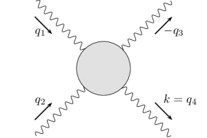
Figure 3: Kinematics of the light-by-light scattering amplitude.

We use the following Lorentz scalars as kinematic variables — these are the usual Mandelstam variables:

$$s:=(q_{1}+q_{2})^{2},\quad t:=(q_{1}+q_{3})^{2},\quad u:=(q_{2}+q_{3})^{2},$$ (3.5)

which fulfill (we will take $k^{2}=0$ at some later point)

$$s+t+u=\sum_{i=1}^{4}q_{i}^{2}=:\Sigma.$$ (3.6)

Gauge invariance requires the HLbL tensor to satisfy the Ward–Takahashi identities

$$\{q_{1}^{\mu},q_{2}^{\nu},q_{3}^{\lambda},q_{4}^{\sigma}\}\Pi_{\mu\nu\lambda\sigma}(q_{1},q_{2},q_{3})=0.$$ (3.7)

3.2 Tensor decomposition

In general, the HLbL tensor can be decomposed into 138 Lorentz structures [44, 45, 13]:

$$\begin{split}\Pi^{\mu\nu\lambda\sigma}&=g^{\mu\nu}g^{\lambda\sigma}\,\Pi^{1}+g^{\mu\lambda}g^{\nu\sigma}\,\Pi^{2}+g^{\mu\sigma}g^{\nu\lambda}\,\Pi^{3}\\ &+\sum_{\begin{subarray}{c}k=1,2,4\\ l=1,2,3\end{subarray}}g^{\mu\nu}q_{k}^{\lambda}q_{l}^{\sigma}\,\Pi^{4}_{kl}+\sum_{\begin{subarray}{c}j=1,3,4\\ l=1,2,3\end{subarray}}g^{\mu\lambda}q_{j}^{\nu}q_{l}^{\sigma}\,\Pi^{5}_{jl}+\sum_{\begin{subarray}{c}j=1,3,4\\ k=1,2,4\end{subarray}}g^{\mu\sigma}q_{j}^{\nu}q_{k}^{\lambda}\,\Pi^{6}_{jk}\\ &+\sum_{\begin{subarray}{c}i=2,3,4\\ l=1,2,3\end{subarray}}g^{\nu\lambda}q_{i}^{\mu}q_{l}^{\sigma}\,\Pi^{7}_{il}+\sum_{\begin{subarray}{c}i=2,3,4\\ k=1,2,4\end{subarray}}g^{\nu\sigma}q_{i}^{\mu}q_{k}^{\lambda}\,\Pi^{8}_{ik}+\sum_{\begin{subarray}{c}i=2,3,4\\ j=1,3,4\end{subarray}}g^{\lambda\sigma}q_{i}^{\mu}q_{j}^{\nu}\,\Pi^{9}_{ij}\\ &+\sum_{\begin{subarray}{c}i=2,3,4\\ j=1,3,4\end{subarray}}\sum_{\begin{subarray}{c}k=1,2,4\\ l=1,2,3\end{subarray}}q_{i}^{\mu}q_{j}^{\nu}q_{k}^{\lambda}q_{l}^{\sigma}\,\Pi^{10}_{ijkl}\\ &=:\sum_{i=1}^{138}L_{i}^{\mu\nu\lambda\sigma}\,\Xi_{i}.\end{split}$$ (3.8)

The 138 scalar functions

$$\{\Xi_{i}\}:=\{\Pi^{1},\Pi^{2},\Pi^{3},\Pi^{4}_{kl},\Pi^{5}_{jl},\Pi^{6}_{jk},\Pi^{7}_{il},\Pi^{8}_{ik},\Pi^{9}_{ij},\Pi^{10}_{ijkl}\}$$ (3.9)

depend on six independent kinematic variables, e.g. on two Mandelstam variables $s$ and $t$ and the virtualities $q_{1}^{2}$, $q_{2}^{2}$, $q_{3}^{2}$, and $q_{4}^{2}$. They are free of kinematic singularities but contain kinematic zeros, because they have to fulfill kinematic constraints required by gauge invariance. The Ward identities (3.7) impose 95 linearly independent relations on the scalar functions, reducing the set to 43 functions.

As we did in Sect. 2.2 for the case of $\gamma^{*}\gamma^{*}\to\pi\pi$, we will now construct a set of Lorentz structures and scalar functions, such that the scalar functions contain neither kinematic singularities nor zeros. Compared to $\gamma^{*}\gamma^{*}\to\pi\pi$, the application of the recipe given by Bardeen, Tung [31], and Tarrach [32] is much more involved. Again, the recipe by Bardeen and Tung does not lead to a kinematic-free minimal basis (which would consist here of 43 scalar functions). Following Tarrach, we will construct a redundant set of 54 structures, which is free of kinematic singularities and zeros.

In a first step, we define the two projectors

$$I_{12}^{\mu\nu}:=g^{\mu\nu}-\frac{q_{2}^{\mu}q_{1}^{\nu}}{q_{1}\cdot q_{2}},\quad I_{34}^{\lambda\sigma}:=g^{\lambda\sigma}-\frac{q_{4}^{\lambda}q_{3}^{\sigma}}{q_{3}\cdot q_{4}},$$ (3.10)

which have the following properties:

$$\begin{aligned} q_{1}^{\mu}I^{12}_{\mu\nu}&=0,\quad&q_{2}^{\nu}I^{12}_{\mu\nu}&=0,\\ q_{3}^{\lambda}I^{34}_{\lambda\sigma}&=0,\quad&q_{4}^{\sigma}I^{34}_{\lambda\sigma}&=0,\\ I_{12}^{\mu\mu^{\prime}}\Pi_{\mu^{\prime}\nu\lambda\sigma}&=\Pi^{\mu}{}_{\nu\lambda\sigma},\quad&I_{12}^{\nu^{\prime}\nu}\Pi_{\mu\nu^{\prime}\lambda\sigma}&=\Pi_{\mu}{}^{\nu}{}_{\lambda\sigma},\\ I_{34}^{\lambda\lambda^{\prime}}\Pi_{\mu\nu\lambda^{\prime}\sigma}&=\Pi_{\mu\nu}{}^{\lambda}{}_{\sigma},\quad&I_{34}^{\sigma^{\prime}\sigma}\Pi_{\mu\nu\lambda\sigma^{\prime}}&=\Pi_{\mu\nu\lambda}{}^{\sigma},\end{aligned}$$

i.e. the HLbL tensor is invariant under contraction with the projectors, but the contraction of every Lorentz structure produces a gauge-invariant structure. Hence, we project the tensor

$$\begin{split}\Pi^{\mu\nu\lambda\sigma}&=I_{12}^{\mu\mu^{\prime}}I_{12}^{\nu^{\prime}\nu}I_{34}^{\lambda\lambda^{\prime}}I_{34}^{\sigma^{\prime}\sigma}\Pi_{\mu^{\prime}\nu^{\prime}\lambda^{\prime}\sigma^{\prime}}\\ &=\sum_{i=1}^{138}I_{12}^{\mu\mu^{\prime}}I_{12}^{\nu^{\prime}\nu}I_{34}^{\lambda\lambda^{\prime}}I_{34}^{\sigma^{\prime}\sigma}L^{i}_{\mu^{\prime}\nu^{\prime}\lambda^{\prime}\sigma^{\prime}}\,\Xi_{i}\\ &=:\sum_{i=1}^{138}\bar{L}_{i}^{\mu\nu\lambda\sigma}\,\Xi_{i}=\sum_{j=1}^{43}\bar{L}_{i_{j}}^{\mu\nu\lambda\sigma}\,\Xi_{i_{j}}.\end{split}$$ (3.12)

Only 43 of the 138 projected structures $\bar{L}_{i}^{\mu\nu\lambda\sigma}$ are non-zero, i.e. all constraints imposed by gauge invariance are already manifestly implemented. Since the projected structures are still multiplied by the original scalar functions $\Xi_{i}$, no kinematic singularities have been introduced into the scalar functions. We now have to remove the kinematic zeros from the scalar functions by removing the single and double poles in $q_{1}\cdot q_{2}$ and $q_{3}\cdot q_{4}$, which are present in the structures $\bar{L}_{i}^{\mu\nu\lambda\sigma}$. We adapt the recipe of [31] (cf. Sect. 2.2):

• remove as many ($q_{1}\cdot q_{2}$, $q_{3}\cdot q_{4}$) double-double poles as possible by adding to the structures linear combinations of other structures with coefficients containing no poles,

• if no more double-double poles can be removed in this way, multiply the structures that still contain double-double poles by either $q_{1}\cdot q_{2}$ or $q_{3}\cdot q_{4}$ (the choice is irrelevant in the end),

• proceed in the same way with double-single, single-double poles, etc. until no poles at all are left in the structures.

As already mentioned, it is again impossible to avoid introducing kinematic singularities into the scalar functions by applying this procedure [32]. However, the only step where kinematic singularities can be introduced is the multiplication of the structures by $q_{1}\cdot q_{2}$ or $q_{3}\cdot q_{4}$ (i.e. the division of the scalar functions by these terms). This means that the only possible singularities are (double or single) poles in $q_{1}\cdot q_{2}$ or $q_{3}\cdot q_{4}$. The precise form of these poles can be easily determined: they correspond to degeneracies of the obtained basis of Lorentz structures in the limit $q_{1}\cdot q_{2}\to 0$ and/or $q_{3}\cdot q_{4}\to 0$. Therefore, the 43-dimensional basis has to be extended by additional structures, which are found by studying the null-space of the present structures in the mentioned limits. 11 such structures can be found. The extended generating set of 54 structures exhibits all possible crossing symmetries in a manifest way.

Explicitly, the resulting representation of the HLbL tensor reads

$$\Pi^{\mu\nu\lambda\sigma} =\sum_{i=1}^{54}T_{i}^{\mu\nu\lambda\sigma}\Pi_{i},$$ (3.13)

where

$$T_{1}^{\mu\nu\lambda\sigma} =\epsilon^{\mu\nu\alpha\beta}\epsilon^{\lambda\sigma\gamma\delta}{q_{1}}_{\alpha}{q_{2}}_{\beta}{q_{3}}_{\gamma}{q_{4}}_{\delta},$$

$$T_{4}^{\mu\nu\lambda\sigma} =\Big{(}q_{2}^{\mu}q_{1}^{\nu}-q_{1}\cdot q_{2}g^{\mu\nu}\Big{)}\Big{(}q_{4}^{\lambda}q_{3}^{\sigma}-q_{3}\cdot q_{4}g^{\lambda\sigma}\Big{)},$$

$$T_{7}^{\mu\nu\lambda\sigma} =\Big{(}q_{2}^{\mu}q_{1}^{\nu}-q_{1}\cdot q_{2}g^{\mu\nu}\Big{)}\Big{(}q_{1}\cdot q_{4}\left(q_{1}^{\lambda}q_{3}^{\sigma}-q_{1}\cdot q_{3}g^{\lambda\sigma}\right)+q_{4}^{\lambda}q_{1}^{\sigma}q_{1}\cdot q_{3}-q_{1}^{\lambda}q_{1}^{\sigma}q_{3}\cdot q_{4}\Big{)},$$

$$T_{19}^{\mu\nu\lambda\sigma} =\Big{(}q_{2}^{\mu}q_{1}^{\nu}-q_{1}\cdot q_{2}g^{\mu\nu}\Big{)}\Big{(}q_{2}\cdot q_{4}\left(q_{1}^{\lambda}q_{3}^{\sigma}-q_{1}\cdot q_{3}g^{\lambda\sigma}\right)+q_{4}^{\lambda}q_{2}^{\sigma}q_{1}\cdot q_{3}-q_{1}^{\lambda}q_{2}^{\sigma}q_{3}\cdot q_{4}\Big{)},$$

$$T_{31}^{\mu\nu\lambda\sigma} =\Big{(}q_{2}^{\mu}q_{1}^{\nu}-q_{1}\cdot q_{2}g^{\mu\nu}\Big{)}\Big{(}q_{2}^{\lambda}q_{1}\cdot q_{3}-q_{1}^{\lambda}q_{2}\cdot q_{3}\Big{)}\Big{(}q_{2}^{\sigma}q_{1}\cdot q_{4}-q_{1}^{\sigma}q_{2}\cdot q_{4}\Big{)},$$

$$T_{37}^{\mu\nu\lambda\sigma} =\Big{(}q_{3}^{\mu}q_{1}\cdot q_{4}-q_{4}^{\mu}q_{1}\cdot q_{3}\Big{)}\begin{aligned} &\Big{(}q_{3}^{\nu}q_{4}^{\lambda}q_{2}^{\sigma}-q_{4}^{\nu}q_{2}^{\lambda}q_{3}^{\sigma}+g^{\lambda\sigma}\left(q_{4}^{\nu}q_{2}\cdot q_{3}-q_{3}^{\nu}q_{2}\cdot q_{4}\right)\\ &+g^{\nu\sigma}\left(q_{2}^{\lambda}q_{3}\cdot q_{4}-q_{4}^{\lambda}q_{2}\cdot q_{3}\right)+g^{\lambda\nu}\left(q_{3}^{\sigma}q_{2}\cdot q_{4}-q_{2}^{\sigma}q_{3}\cdot q_{4}\right)\Big{)},\end{aligned}$$

$$T_{49}^{\mu\nu\lambda\sigma} =q_{3}^{\sigma}\begin{aligned} &\Big{(}q_{1}\cdot q_{3}q_{2}\cdot q_{4}q_{4}^{\mu}g^{\lambda\nu}-q_{2}\cdot q_{3}q_{1}\cdot q_{4}q_{4}^{\nu}g^{\lambda\mu}+q_{4}^{\mu}q_{4}^{\nu}\left(q_{1}^{\lambda}q_{2}\cdot q_{3}-q_{2}^{\lambda}q_{1}\cdot q_{3}\right)\\ &+q_{1}\cdot q_{4}q_{3}^{\mu}q_{4}^{\nu}q_{2}^{\lambda}-q_{2}\cdot q_{4}q_{4}^{\mu}q_{3}^{\nu}q_{1}^{\lambda}+q_{1}\cdot q_{4}q_{2}\cdot q_{4}\left(q_{3}^{\nu}g^{\lambda\mu}-q_{3}^{\mu}g^{\lambda\nu}\right)\Big{)}\end{aligned}$$

$$-q_{4}^{\lambda}\begin{aligned} &\Big{(}q_{1}\cdot q_{4}q_{2}\cdot q_{3}q_{3}^{\mu}g^{\nu\sigma}-q_{2}\cdot q_{4}q_{1}\cdot q_{3}q_{3}^{\nu}g^{\mu\sigma}+q_{3}^{\mu}q_{3}^{\nu}\left(q_{1}^{\sigma}q_{2}\cdot q_{4}-q_{2}^{\sigma}q_{1}\cdot q_{4}\right)\\ &+q_{1}\cdot q_{3}q_{4}^{\mu}q_{3}^{\nu}q_{2}^{\sigma}-q_{2}\cdot q_{3}q_{3}^{\mu}q_{4}^{\nu}q_{1}^{\sigma}+q_{1}\cdot q_{3}q_{2}\cdot q_{3}\left(q_{4}^{\nu}g^{\mu\sigma}-q_{4}^{\mu}g^{\nu\sigma}\right)\Big{)}\end{aligned}$$

$$+q_{3}\cdot q_{4}\Big{(}\left(q_{1}^{\lambda}q_{4}^{\mu}-q_{1}\cdot q_{4}g^{\lambda\mu}\right)\left(q_{3}^{\nu}q_{2}^{\sigma}-q_{2}\cdot q_{3}g^{\nu\sigma}\right)-\left(q_{2}^{\lambda}q_{4}^{\nu}-q_{2}\cdot q_{4}g^{\lambda\nu}\right)\left(q_{3}^{\mu}q_{1}^{\sigma}-q_{1}\cdot q_{3}g^{\mu\sigma}\right)\Big{)}.\quad$$

These structures satisfy the following crossing symmetries:

$$T_{1}^{\mu\nu\lambda\sigma} =\mathcal{C}_{12}[T_{1}^{\mu\nu\lambda\sigma}]=\mathcal{C}_{34}[T_{1}^{\mu\nu\lambda\sigma}]=\mathcal{C}_{34}[\mathcal{C}_{12}[T_{1}^{\mu\nu\lambda\sigma}]]=\mathcal{C}_{24}[\mathcal{C}_{13}[T_{1}^{\mu\nu\lambda\sigma}]]$$

$$=\mathcal{C}_{23}[\mathcal{C}_{14}[T_{1}^{\mu\nu\lambda\sigma}]]=\mathcal{C}_{24}[\mathcal{C}_{13}[\mathcal{C}_{34}[T_{1}^{\mu\nu\lambda\sigma}]]]=\mathcal{C}_{23}[\mathcal{C}_{14}[\mathcal{C}_{34}[T_{1}^{\mu\nu\lambda\sigma}]]],$$

$$T_{4}^{\mu\nu\lambda\sigma} =\mathcal{C}_{12}[T_{4}^{\mu\nu\lambda\sigma}]=\mathcal{C}_{34}[T_{4}^{\mu\nu\lambda\sigma}]=\mathcal{C}_{34}[\mathcal{C}_{12}[T_{4}^{\mu\nu\lambda\sigma}]]=\mathcal{C}_{24}[\mathcal{C}_{13}[T_{4}^{\mu\nu\lambda\sigma}]]$$

$$=\mathcal{C}_{23}[\mathcal{C}_{14}[T_{4}^{\mu\nu\lambda\sigma}]]=\mathcal{C}_{24}[\mathcal{C}_{13}[\mathcal{C}_{34}[T_{4}^{\mu\nu\lambda\sigma}]]]=\mathcal{C}_{23}[\mathcal{C}_{14}[\mathcal{C}_{34}[T_{4}^{\mu\nu\lambda\sigma}]]],$$

$$T_{7}^{\mu\nu\lambda\sigma} =\mathcal{C}_{34}[T_{7}^{\mu\nu\lambda\sigma}],$$

$$T_{19}^{\mu\nu\lambda\sigma} =\mathcal{C}_{34}[\mathcal{C}_{12}[T_{19}^{\mu\nu\lambda\sigma}]],$$

$$T_{31}^{\mu\nu\lambda\sigma} =\mathcal{C}_{12}[T_{31}^{\mu\nu\lambda\sigma}]=\mathcal{C}_{34}[T_{31}^{\mu\nu\lambda\sigma}]=\mathcal{C}_{34}[\mathcal{C}_{12}[T_{31}^{\mu\nu\lambda\sigma}]],$$

$$T_{37}^{\mu\nu\lambda\sigma} =\mathcal{C}_{34}[T_{37}^{\mu\nu\lambda\sigma}],$$

$$T_{49}^{\mu\nu\lambda\sigma} =-\mathcal{C}_{12}[T_{49}^{\mu\nu\lambda\sigma}]=-\mathcal{C}_{34}[T_{49}^{\mu\nu\lambda\sigma}]=\mathcal{C}_{34}[\mathcal{C}_{12}[T_{49}^{\mu\nu\lambda\sigma}]],$$

where the crossing operators $\mathcal{C}_{ij}$ exchange momenta and Lorentz indices of the photons $i$ and $j$, e.g.

$$\mathcal{C}_{12}[f]:=f(\mu\leftrightarrow\nu,q_{1}\leftrightarrow q_{2}),\quad\mathcal{C}_{14}[f]:=f(\mu\leftrightarrow\sigma,q_{1}\leftrightarrow-q_{4}).$$ (3.16)

All the remaining structures are just crossed versions of the above seven structures, as shown in App. B.1. Since the HLbL tensor $\Pi^{\mu\nu\lambda\sigma}$ is totally crossing symmetric, the scalar functions $\Pi_{i}$ have to fulfill exactly the same crossing properties of the corresponding Lorentz structures as given in (3.2) (note the antisymmetric crossing relations in $\Pi_{49}$). Therefore, only seven different scalar functions $\Pi_{i}$ appear, together with their crossed versions. These scalar functions are free of kinematic singularities and zeros and hence fulfill a Mandelstam representation. They are suitable quantities for a dispersive description.

The subset consisting of the following 43 Lorentz structures forms a basis:

$$\{\mathcal{B}^{\mu\nu\lambda\sigma}_{i}\}:=\Big{\{}T^{\mu\nu\lambda\sigma}_{i}\big{|}i\in\{1,\ldots,21,23,25,27,29,30,33,\ldots,36,38,\ldots,45,49,\ldots,53\}\Big{\}}.$$ (3.17)

The corresponding scalar coefficient functions $\tilde{\Pi}_{i}$, defined by

$$\Pi^{\mu\nu\lambda\sigma} =\sum_{i=1}^{43}\mathcal{B}_{i}^{\mu\nu\lambda\sigma}\tilde{\Pi}_{i},$$ (3.18)

exhibit kinematic singularities in $q_{1}\cdot q_{2}$ and $q_{3}\cdot q_{4}$. The exact form of these kinematic singularities can be determined by projecting (3.13) on this basis. The relation between the basis coefficient functions $\tilde{\Pi}_{i}$ and the scalar functions $\Pi_{i}$ is given in App. B.2.

While crossing symmetry is manifest if the HLbL tensor is expressed in terms of the redundant set of 54 structures, it is partially obscured in the basis of 43 elements. Still, many basis functions $\tilde{\Pi}_{i}$ are related by crossing symmetry, see (B.2) in App. B.2. The basis coefficient functions are completely specified by crossing symmetry and 9 representative functions, e.g.

$$\left\{\tilde{\Pi}_{1},\tilde{\Pi}_{4},\tilde{\Pi}_{7},\tilde{\Pi}_{9},\tilde{\Pi}_{19},\tilde{\Pi}_{21},\tilde{\Pi}_{36},\tilde{\Pi}_{39},\tilde{\Pi}_{40}\right\}.$$ (3.19)

We stress again that our decomposition (3.13) is both manifestly crossing symmetric and gauge invariant. In particular, this implies that all soft-photon zeros [39] of the helicity amplitudes (3.3) are already implemented, in contrast to the helicity basis employed in [26]. In this case, only specific combinations of basis functions were free of kinematic singularities and zeros and thus admitted a dispersive representation, while the soft-photon constraints needed to be imposed by hand. The BTT set (3.2) provides a Lorentz decomposition that incorporates soft-photon constraints and avoids kinematics by construction. On the other hand, the main motivation for choosing the helicity basis was that the unitarity relations in the form of helicity partial-wave amplitudes become diagonal. Of course, this will not be true in the BTT basis, so that the derivation of an explicit dispersive representation for the BTT amplitudes requires a basis change. In practice, this change between BTT and helicity bases proceeds by means of (3.8) as an intermediate step: the helicity amplitudes can be easily expressed in terms of (3.8), while the remaining basis change can be performed along the lines explained in App. C.

3.3 Redundancies in the Lorentz decomposition

Because the set of 54 scalar functions is redundant, there is obviously an ambiguity in the definition of the coefficient functions. However, crossing symmetry and the absence of kinematic singularities restrict this ambiguity in a very specific way. The shifts

$$\Pi_{i}\mapsto\Pi_{i}+\delta\Pi_{i}$$ (3.20)

leaving the HLbL tensor $\Pi^{\mu\nu\lambda\sigma}$ invariant are easily found by requiring that the basis elements $\tilde{\Pi}_{i}$ remain invariant. We find

$$\begin{aligned} \delta\Pi_{1}&=0,\quad&\delta\Pi_{4}&=0,\\ \delta\Pi_{7}&=-q_{2}\cdot q_{3}q_{2}\cdot q_{4}\Delta_{19},\quad&\delta\Pi_{19}&=q_{1}\cdot q_{4}q_{2}\cdot q_{3}\Delta_{19},\quad&\delta\Pi_{31}&=-q_{3}\cdot q_{4}\Delta_{19},\\ \delta\Pi_{37}&=q_{1}\cdot q_{2}\Delta_{37},\quad&\delta\Pi_{49}&=q_{1}\cdot q_{2}\Delta_{49},\end{aligned}$$ (3.21)

where the shifts have to satisfy

$$\begin{split}\Delta_{19}&=\mathcal{C}_{12}[\Delta_{19}]=\mathcal{C}_{34}[\Delta_{19}]=\mathcal{C}_{34}[\mathcal{C}_{12}[\Delta_{19}]],\\ \Delta_{37}&=\mathcal{C}_{24}[\Delta_{37}]=\mathcal{C}_{23}[\Delta_{37}]=\mathcal{C}_{34}[\Delta_{37}]=\mathcal{C}_{24}[\mathcal{C}_{34}[\Delta_{37}]]=\mathcal{C}_{24}[\mathcal{C}_{23}[\Delta_{37}]],\\ \Delta_{49}&=-\mathcal{C}_{12}[\Delta_{49}]=-\mathcal{C}_{13}[\Delta_{49}]=-\mathcal{C}_{14}[\Delta_{49}]=-\mathcal{C}_{23}[\Delta_{49}]=-\mathcal{C}_{24}[\Delta_{49}]=-\mathcal{C}_{34}[\Delta_{49}]=\ldots.\end{split}$$ (3.22)

The ellipses in the last line stand for the permutations that are not listed explicitly: $\Delta_{49}$ is symmetric (antisymmetric) under all even (odd) crossing permutations. The shifts $\delta\Pi_{i}$ that are not specified follow from the crossing relations (B.1).

Apart from the redundancy introduced by extending the basis to a set of 54 elements, there exists another ambiguity in the definition of the scalar function. As it was pointed out in [46], the 138 initial Lorentz structures of the HLbL tensor fulfill two linear relations in $d=4$ space-time dimensions. This is not obvious in a covariant notation, but can be easily shown in an explicit reference frame. The two linear relations can be translated into two linear relations between the 43 basis elements (which means that these structures actually do not form a basis in a strict sense). Therefore, in four space-time dimensions there are only 41 independent scalar functions, which matches the number of fully off-shell helicity amplitudes. This is analogous to the case of $\gamma^{*}\gamma^{*}\to\pi\pi$, where the number of helicity amplitudes ($5$) also matches the number of independent scalar functions.

The two linear relations can be further translated into relations amongst the 54 elements of the redundant crossing-symmetric set of Lorentz structures. In fact, it turns out that expressed in this way, the two relations become particularly simple. They are given by:

$$\sum_{i=1}^{54}c_{i}^{1,2}T_{i}^{\mu\nu\lambda\sigma}=0,$$ (3.23)

where

$$\begin{split}c^{1}_{1}&=-s+t+u,\quad c^{1}_{3}=-s-t+u,\quad c^{1}_{4}=-5s-t+u,\quad c^{1}_{5}=2(-s+u),\quad c^{1}_{6}=-s+t+5u,\\ c^{1}_{7}&=c^{1}_{8}=c^{1}_{17}=c^{1}_{18}=c^{1}_{19}=c^{1}_{20}=c^{1}_{29}=c^{1}_{30}=c^{1}_{50}=c^{1}_{53}=4,\\ c^{1}_{11}&=c^{1}_{12}=c^{1}_{13}=c^{1}_{14}=c^{1}_{23}=c^{1}_{24}=c^{1}_{25}=c^{1}_{26}=-4,\\ c^{1}_{37}&=c^{1}_{46}=c^{1}_{47}=c^{1}_{48}=c^{1}_{51}=c^{1}_{52}=2,\\ c^{1}_{38}&=c^{1}_{40}=c^{1}_{43}=c^{1}_{44}=c^{1}_{49}=c^{1}_{54}=-2,\end{split}$$ (3.24)

and

$$\begin{split}c^{2}_{2}&=s-t+u,\quad c^{2}_{3}=-s-t+u,\quad c^{2}_{4}=2(-t+u),\quad c^{2}_{5}=-s-5t+u,\quad c^{2}_{6}=s-t+5u,\\ c^{2}_{9}&=c^{2}_{10}=c^{2}_{15}=c^{2}_{16}=c^{2}_{21}=c^{2}_{22}=c^{2}_{27}=c^{2}_{28}=4,\\ c^{2}_{11}&=c^{2}_{12}=c^{2}_{13}=c^{2}_{14}=c^{2}_{14}=c^{2}_{23}=c^{2}_{24}=c^{2}_{25}=c^{2}_{26}=c^{2}_{49}=c^{2}_{54}=-4\\ c^{2}_{38}&=c^{2}_{40}=c^{2}_{43}=c^{2}_{44}=c^{2}_{51}=c^{2}_{52}=-2,\\ c^{2}_{39}&=c^{2}_{41}=c^{2}_{42}=c^{2}_{45}=c^{2}_{50}=c^{2}_{53}=2,\end{split}$$ (3.25)

and where all unspecified $c_{i}^{1,2}$ are zero. Eq. (3.23) is most easily verified by contracting the equation with the 138 tensor structures. We have checked explicitly that the matrix $\{L_{i}^{\mu\nu\lambda\sigma}L_{\mu\nu\lambda\sigma}^{k}\}_{ik}$ is of rank 136. The linear relations between the structures imply the following ambiguities in the scalar functions:

$$\Pi_{i}\mapsto\Pi_{i}+c_{i}^{1}f_{1}+c_{i}^{2}f_{2},$$ (3.26)

where $f_{1,2}$ are a priori unspecified functions free of kinematic singularities. The requirement that the scalar functions satisfy crossing relations of the same form as (3.2) and (B.1) imposes crossing relations on the functions $f_{1,2}$:

$$f_{1} =\mathcal{C}_{12}[f_{2}]=\mathcal{C}_{34}[\mathcal{C}_{12}[f_{1}]]=\mathcal{C}_{24}[\mathcal{C}_{13}[f_{1}]]=\mathcal{C}_{14}[f_{1}]=-\mathcal{C}_{12}[f_{1}]-\mathcal{C}_{13}[f_{1}].$$ (3.27)

Let us write

$$\begin{split}\Pi_{49}&=\frac{1}{4}\left(\Pi_{49}+\mathcal{C}_{24}[\mathcal{C}_{13}[\Pi_{49}]]+\mathcal{C}_{14}[\Pi_{49}]+\mathcal{C}_{14}[\mathcal{C}_{24}[\mathcal{C}_{13}[\Pi_{49}]]]\right)\\ &+\frac{1}{4}\left(\Pi_{49}+\mathcal{C}_{24}[\mathcal{C}_{13}[\Pi_{49}]]-\mathcal{C}_{14}[\Pi_{49}]-\mathcal{C}_{14}[\mathcal{C}_{24}[\mathcal{C}_{13}[\Pi_{49}]]]\right)\\ &+\frac{1}{2}\left(\Pi_{49}-\mathcal{C}_{24}[\mathcal{C}_{13}[\Pi_{49}]]\right).\end{split}$$ (3.28)

The first bracket in this expression is given by $\Pi_{49}-\Pi_{50}-\Pi_{53}+\Pi_{54}$ and has exactly the crossing properties of $f_{1}$. Therefore, the ambiguity can be fixed by the condition

$$\Pi_{49}-\Pi_{50}-\Pi_{53}+\Pi_{54}=0.$$ (3.29)

Very recently, a Lorentz decomposition of the HLbL tensor into 72 redundant structures has been presented in [47]. A comparison with our redundant set of 54 structures, as first given in [33], has been performed, confirming the absence of kinematic singularities. By studying systematically the irreducible representations of the permutation group $S_{4}$, the authors of [47] aim at constructing a minimal basis consisting of 41 totally crossing symmetric elements free of kinematic singularities. Note, however, that [47] neither provides this basis nor a concrete recipe for how to obtain it. Therefore, it remains to be seen if a minimal basis free of kinematic singularities exists at all. For our purpose the question whether such a basis exists is immaterial, since for a dispersive representation of the HLbL tensor all that is required is a decomposition into scalar amplitudes free of kinematic zeros and singularities.

To conclude this subsection, we stress that the presence of kinematic singularities in any known basis requires us to work with a redundant set of $54$ Lorentz structures and scalar functions $\Pi_{i}$. Although the redundancy of the Lorentz structures introduces an ambiguity in the functions $\Pi_{i}$ (which is already very restricted by crossing symmetry and will be further restricted by analyticity), this ambiguity will cancel in the calculation of any physical quantity such as $(g-2)_{\mu}$. In particular, this implies that the additional redundancy in $d=4$ dimensions does not affect our calculation in any way, since the minimal set suited for a dispersive representation still involves $54$ functions. In the rest of the paper we will continue to work with the BTT amplitudes defined in (3.2).

4 HLbL contribution to $\boldsymbol{(g-2)_{\mu}}$

In Sect. 4.1, we review the definition and calculation of $a_{\mu}$, as well as general techniques for the calculation of $a_{\mu}^{\text{HLbL}}$ (see e.g. [48]). The well-known general formula requires still a rather long calculation before a number can be finally obtained. For the pion-pole contribution, these steps have been worked out long ago [19]. With our complete set of 54 kinematic-free structures (3.13), this procedure can be repeated for the whole HLbL contribution in full generality, as we explain in Sects. 4.2 and 4.3. In Sect. 4.4, we study the validity of the applied Wick rotation in the presence of anomalous thresholds.

4.1 Projector techniques

The $T$-matrix element of the interaction of a muon with the electromagnetic field is defined by

$$\mathcal{T}^{\mu}(p_{1},p_{2}):=-e\langle\mu^{-}(p_{2},s_{2})|j_{\mathrm{em}}^{\mu}(0)|\mu^{-}(p_{1},s_{1})\rangle,$$ (4.1)

where $e=|e|$. Diagrammatically

$$\begin{minipage}{56.9055pt} \includegraphics[height=56.9055pt]{images/MuMuGamma} \end{minipage}=i\mathcal{T}^{\mu}(p_{1},p_{2})=(-ie)\bar{u}(p_{2})\Gamma^{\mu}(p_{1},p_{2})u(p_{1}).$$ (4.2)

Assuming parity conservation, the vertex function $\Gamma^{\mu}$ can be decomposed into form factors as

$$\Gamma^{\mu}(p_{1},p_{2}) =\gamma^{\mu}F_{1}(k^{2})-i\frac{\sigma^{\mu\nu}k_{\nu}}{2m_{\mu}}F_{2}(k^{2}),$$ (4.3)

where $k=p_{1}-p_{2}$ and $\sigma^{\mu\nu}:=\frac{i}{2}[\gamma^{\mu},\gamma^{\nu}]$. $F_{1}$ is the electric charge or Dirac form factor, $F_{2}$ the magnetic or Pauli form factor. The anomalous magnetic moment of the muon is given by

$$a_{\mu}=\frac{1}{2}(g-2)_{\mu}=F_{2}(0).$$ (4.4)

We expand the vertex function $\Gamma^{\mu}$ to first order in powers of $k^{\mu}$:

$$\begin{split}\Gamma^{\mu}(p_{1},p_{2})&=\Gamma^{\mu}(p,p)+k_{\nu}\frac{\partial}{\partial k_{\nu}}\Gamma^{\mu}(p_{1},p_{2})\bigg{|}_{k=0}+\ldots\\ &=:V^{\mu}(p)+k_{\nu}\Gamma^{\mu\nu}(p)+\ldots,\end{split}$$ (4.5)

where $p:=\frac{1}{2}(p_{1}+p_{2})$.

Using projector techniques together with angular averages (see [19, 48]), the anomalous magnetic moment of the muon can be calculated as

$$\begin{split}a_{\mu}&=\mathrm{Tr}\left(\left(\frac{1}{12}\gamma^{\mu}-\frac{1}{3}\left(\frac{p^{\mu}\not{p}}{m_{\mu}^{2}}\right)-\frac{1}{4}\frac{p^{\mu}}{m_{\mu}}\right)V_{\mu}(p)\right)\\ &-\frac{1}{48m_{\mu}}\mathrm{Tr}\left((\not{p}+m_{\mu})[\gamma^{\mu},\gamma^{\rho}](\not{p}+m_{\mu})\Gamma_{\mu\rho}(p)\right),\end{split}$$ (4.6)

where now $p^{2}=m_{\mu}^{2}$.

We are interested in the contribution of the HLbL tensor to $a_{\mu}$, diagrammatically

$$\begin{minipage}{56.9055pt} \includegraphics[height=56.9055pt]{images/MuMuGammaHLbL} \end{minipage}=(-ie)\bar{u}(p_{2})\Gamma^{\mu}_{\mathrm{HLbL}}(p_{1},p_{2})u(p_{1}),$$ (4.7)

where

$$\begin{split}\Gamma^{\sigma}_{\mathrm{HLbL}}(p_{1},p_{2})&=-e^{6}\int\frac{d^{4}q_{1}}{(2\pi)^{4}}\frac{d^{4}q_{2}}{(2\pi)^{4}}\gamma_{\mu}\frac{(\not{p}_{2}+\not{q}_{1}+m_{\mu})}{(p_{2}+q_{1})^{2}-m_{\mu}^{2}}\gamma_{\lambda}\frac{(\not{p}_{1}-\not{q}_{2}+m_{\mu})}{(p_{1}-q_{2})^{2}-m_{\mu}^{2}}\gamma_{\nu}\\ &\quad\times\frac{1}{q_{1}^{2}q_{2}^{2}(p_{1}-p_{2}-q_{1}-q_{2})^{2}}\Pi^{\mu\nu\lambda\sigma}(q_{1},q_{2},p_{1}-p_{2}-q_{1}-q_{2}).\end{split}$$ (4.8)

The HLbL tensor is defined in (3.1). Differentiating the fourth Ward identity in (3.7) with respect to $k_{\rho}=(q_{1}+q_{2}+q_{3})_{\rho}$ yields

$$\Pi_{\mu\nu\lambda\rho}(q_{1},q_{2},k-q_{1}-q_{2})=-k^{\sigma}\frac{\partial}{\partial k^{\rho}}\Pi_{\mu\nu\lambda\sigma}(q_{1},q_{2},k-q_{1}-q_{2}).$$ (4.9)

It was already argued in [49] that $\Pi_{\mu\nu\lambda\sigma}$ vanishes linearly with $k$ (i.e. the derivative contains no singularity), and so must $\Gamma_{\sigma}^{\mathrm{HLbL}}$. This is easily verified with our tensor decomposition (3.13). Therefore, the HLbL contribution to the anomalous magnetic moment is given by

$$a_{\mu}^{\mathrm{HLbL}}=-\frac{1}{48m_{\mu}}\mathrm{Tr}\left((\not{p}+m_{\mu})[\gamma^{\rho},\gamma^{\sigma}](\not{p}+m_{\mu})\Gamma_{\rho\sigma}^{\mathrm{HLbL}}(p)\right),$$ (4.10)

where

$$\Gamma^{\mathrm{HLbL}}_{\rho\sigma}(p)=\frac{\partial}{\partial k^{\sigma}}\Gamma^{\mathrm{HLbL}}_{\rho}(p_{1},p_{2})\bigg{|}_{k=0}.$$ (4.11)

We use the Ward identity (4.9) to write

$$\begin{split}\Gamma_{\rho}^{\mathrm{HLbL}}(p_{1},p_{2})&=e^{6}\int\frac{d^{4}q_{1}}{(2\pi)^{4}}\frac{d^{4}q_{2}}{(2\pi)^{4}}\gamma^{\mu}\frac{(\not{p}_{2}+\not{q}_{1}+m_{\mu})}{(p_{2}+q_{1})^{2}-m_{\mu}^{2}}\gamma^{\lambda}\frac{(\not{p}_{1}-\not{q}_{2}+m_{\mu})}{(p_{1}-q_{2})^{2}-m_{\mu}^{2}}\gamma^{\nu}\\ &\quad\times\frac{1}{q_{1}^{2}q_{2}^{2}(p_{1}-p_{2}-q_{1}-q_{2})^{2}}k^{\sigma}\frac{\partial}{\partial k^{\rho}}\Pi_{\mu\nu\lambda\sigma}(q_{1},q_{2},k-q_{1}-q_{2}).\end{split}$$ (4.12)

Taking the derivative and limit leads to the well-known expression

$$\begin{split}\Gamma_{\rho\sigma}^{\mathrm{HLbL}}(p)&=e^{6}\int\frac{d^{4}q_{1}}{(2\pi)^{4}}\frac{d^{4}q_{2}}{(2\pi)^{4}}\gamma^{\mu}\frac{(\not{p}+\not{q}_{1}+m_{\mu})}{(p+q_{1})^{2}-m_{\mu}^{2}}\gamma^{\lambda}\frac{(\not{p}-\not{q}_{2}+m_{\mu})}{(p-q_{2})^{2}-m_{\mu}^{2}}\gamma^{\nu}\\ &\quad\times\frac{1}{q_{1}^{2}q_{2}^{2}(q_{1}+q_{2})^{2}}\frac{\partial}{\partial k^{\rho}}\Pi_{\mu\nu\lambda\sigma}(q_{1},q_{2},k-q_{1}-q_{2})\bigg{|}_{k=0}.\end{split}$$ (4.13)

4.2 Loop integration

In order to compute the contribution to $(g-2)_{\mu}$, one has to take the trace in (4.10) and perform the two-loop integral of equation (4.13). Five of the eight integrals can be carried out analytically with the help of Gegenbauer polynomial techniques [50]. To this end, we employ the representation of the HLbL tensor in terms of the 54 Lorentz structures $T_{i}^{\mu\nu\lambda\sigma}$:

$$\begin{split}a_{\mu}^{\mathrm{HLbL}}&=-\frac{e^{6}}{48m_{\mu}}\int\frac{d^{4}q_{1}}{(2\pi)^{4}}\frac{d^{4}q_{2}}{(2\pi)^{4}}\frac{1}{q_{1}^{2}q_{2}^{2}(q_{1}+q_{2})^{2}}\frac{1}{(p+q_{1})^{2}-m_{\mu}^{2}}\frac{1}{(p-q_{2})^{2}-m_{\mu}^{2}}\\ &\quad\times\mathrm{Tr}\left((\not{p}+m_{\mu})[\gamma^{\rho},\gamma^{\sigma}](\not{p}+m_{\mu})\gamma^{\mu}(\not{p}+\not{q}_{1}+m_{\mu})\gamma^{\lambda}(\not{p}-\not{q}_{2}+m_{\mu})\gamma^{\nu}\right)\\ &\quad\times\sum_{i=1}^{54}\left(\frac{\partial}{\partial k^{\rho}}T^{i}_{\mu\nu\lambda\sigma}(q_{1},q_{2},k-q_{1}-q_{2})\right)\bigg{|}_{k=0}\Pi_{i}(q_{1},q_{2},-q_{1}-q_{2}).\end{split}$$ (4.14)

It turns out that there are only 19 independent linear combinations of the structures $T_{i}^{\mu\nu\lambda\sigma}$ that contribute to $(g-2)_{\mu}$. It is possible to make a basis change in the 54 structures

$$\Pi^{\mu\nu\lambda\sigma}=\sum_{i=1}^{54}T_{i}^{\mu\nu\lambda\sigma}\Pi_{i}=\sum_{i=1}^{54}\hat{T}_{i}^{\mu\nu\lambda\sigma}\hat{\Pi}_{i},$$ (4.15)

in such a way that in the limit $k\to 0$ the derivative of 35 structures $\hat{T}_{i}^{\mu\nu\lambda\sigma}$ vanishes. Although this change of basis does not introduce kinematic singularities into the scalar functions $\hat{\Pi}_{i}$, it somewhat obscures crossing symmetry. The 19 structures $\hat{T}_{i}^{\mu\nu\lambda\sigma}$ that contribute to $(g-2)_{\mu}$ can be chosen as follows:

$$\begin{split}\left\{\hat{T}_{i}^{\mu\nu\lambda\sigma}\Big{|}i=1,\ldots,19\right\}&=\left\{T_{i}^{\mu\nu\lambda\sigma}\Big{|}i=1,\ldots,11,13,14,16,17\right\}\\ &\qquad\cup\left\{T_{39}^{\mu\nu\lambda\sigma}+T_{40}^{\mu\nu\lambda\sigma},T_{42}^{\mu\nu\lambda\sigma},T_{43}^{\mu\nu\lambda\sigma},T_{50}^{\mu\nu\lambda\sigma}-T_{51}^{\mu\nu\lambda\sigma}\right\}.\end{split}$$ (4.16)

The corresponding 19 scalar functions $\hat{\Pi}_{i}$ are linear combinations of 33 scalar functions $\Pi_{i}$, see App. D. The 21 scalar functions not involved in these relations

$$\left\{\Pi_{i}\Big{|}i=12,15,18,23,24,27,28,29,30,32,35,36,37,38,41,44,45,48,49,52,53\right\}$$ (4.17)

are irrelevant for the calculation of $(g-2)_{\mu}$.

The HLbL contribution to $(g-2)_{\mu}$ can now be written as

$$\begin{split}a_{\mu}^{\mathrm{HLbL}}&=-e^{6}\int\frac{d^{4}q_{1}}{(2\pi)^{4}}\frac{d^{4}q_{2}}{(2\pi)^{4}}\frac{1}{q_{1}^{2}q_{2}^{2}(q_{1}+q_{2})^{2}}\frac{1}{(p+q_{1})^{2}-m_{\mu}^{2}}\frac{1}{(p-q_{2})^{2}-m_{\mu}^{2}}\\ &\quad\times\sum_{i=1}^{19}\hat{T}_{i}(q_{1},q_{2};p)\hat{\Pi}_{i}(q_{1},q_{2},-q_{1}-q_{2}),\end{split}$$ (4.18)

where

$$\begin{split}\hat{T}_{i}(q_{1},q_{2};p):=\frac{1}{48m_{\mu}}\mathrm{Tr}&\left((\not{p}+m_{\mu})[\gamma^{\rho},\gamma^{\sigma}](\not{p}+m_{\mu})\gamma^{\mu}(\not{p}+\not{q}_{1}+m_{\mu})\gamma^{\lambda}(\not{p}-\not{q}_{2}+m_{\mu})\gamma^{\nu}\right)\\ &\times\left(\frac{\partial}{\partial k^{\rho}}\hat{T}^{i}_{\mu\nu\lambda\sigma}(q_{1},q_{2},k-q_{1}-q_{2})\right)\bigg{|}_{k=0}\end{split}$$ (4.19)

and the $\hat{\Pi}_{i}$ are needed for the reduced kinematics

$$s=(q_{1}+q_{2})^{2},\quad t=q_{2}^{2},\quad u=q_{1}^{2},\quad q_{1}^{2},\quad q_{2}^{2},\quad q_{3}^{2}=(q_{1}+q_{2})^{2},\quad k^{2}=q_{4}^{2}=0.$$ (4.20)

The explicit result of the trace calculation and the contraction of the Lorentz indices is given in App. E.1.

We can reduce the number of terms contributing to $(g-2)_{\mu}$ further by using the symmetry under the exchange of the momenta $q_{1}\leftrightarrow-q_{2}$: the loop integration measure and the product of propagators are invariant under this transformation, while the kernels $\hat{T}_{i}$ transform under $q_{1}\leftrightarrow-q_{2}$ as

$$\begin{aligned} \hat{T}_{1}&\longleftrightarrow\hat{T}_{1},\quad&\hat{T}_{2}&\longleftrightarrow\hat{T}_{3},\quad&\hat{T}_{4}&\longleftrightarrow\hat{T}_{4},\quad&\hat{T}_{5}&\longleftrightarrow\hat{T}_{6},\\ \hat{T}_{7}&\longleftrightarrow\hat{T}_{8},\quad&\hat{T}_{9}&\longleftrightarrow\hat{T}_{12},\quad&\hat{T}_{10}&\longleftrightarrow\hat{T}_{13},\quad&\hat{T}_{11}&\longleftrightarrow\hat{T}_{14},\\ \hat{T}_{15}&\longleftrightarrow\hat{T}_{15},\quad&\hat{T}_{16}&\longleftrightarrow\hat{T}_{16},\quad&\hat{T}_{17}&\longleftrightarrow\hat{T}_{18},\quad&\hat{T}_{19}&\longleftrightarrow-\hat{T}_{19}.\end{aligned}$$

For the reduced kinematics (4.20) the exchange $q_{1}\leftrightarrow-q_{2}$ is equivalent to the crossing transformation $t\leftrightarrow u$, $q_{1}^{2}\leftrightarrow q_{2}^{2}$. With the help of the crossing relations of the scalar functions $\Pi_{i}$, it is easy to check that the $\vphantom{\Big{|}}\hat{\Pi}_{i}$ transform analogously to the kernels $\hat{T}_{i}$, i.e.

$$\begin{aligned} \hat{\Pi}_{1}&\longleftrightarrow\hat{\Pi}_{1},\quad&\hat{\Pi}_{2}&\longleftrightarrow\hat{\Pi}_{3},\quad&\hat{\Pi}_{4}&\longleftrightarrow\hat{\Pi}_{4},\quad&\hat{\Pi}_{5}&\longleftrightarrow\hat{\Pi}_{6},\\ \hat{\Pi}_{7}&\longleftrightarrow\hat{\Pi}_{8},\quad&\hat{\Pi}_{9}&\longleftrightarrow\hat{\Pi}_{12},\quad&\hat{\Pi}_{10}&\longleftrightarrow\hat{\Pi}_{13},\quad&\hat{\Pi}_{11}&\longleftrightarrow\hat{\Pi}_{14},\\ \hat{\Pi}_{15}&\longleftrightarrow\hat{\Pi}_{15},\quad&\hat{\Pi}_{16}&\longleftrightarrow\hat{\Pi}_{16},\quad&\hat{\Pi}_{17}&\longleftrightarrow\hat{\Pi}_{18},\quad&\hat{\Pi}_{19}&\longleftrightarrow-\hat{\Pi}_{19}.\end{aligned}$$

Therefore, it is convenient to write the HLbL contribution to $(g-2)_{\mu}$ as a sum of 12 terms:

$$\begin{split}a_{\mu}^{\mathrm{HLbL}}&=-e^{6}\int\frac{d^{4}q_{1}}{(2\pi)^{4}}\frac{d^{4}q_{2}}{(2\pi)^{4}}\frac{1}{q_{1}^{2}q_{2}^{2}(q_{1}+q_{2})^{2}}\frac{1}{(p+q_{1})^{2}-m_{\mu}^{2}}\frac{1}{(p-q_{2})^{2}-m_{\mu}^{2}}\\ &\quad\times\sum_{j=1}^{12}\xi_{j}\hat{T}_{i_{j}}(q_{1},q_{2};p)\hat{\Pi}_{i_{j}}(q_{1},q_{2},-q_{1}-q_{2}),\end{split}$$ (4.23)

where

$$\begin{split}\{i_{j}|j=1,\ldots,12\}&=\{1,2,4,5,7,9,10,14,15,16,17,19\},\\ \{\xi_{j}|j=1,\ldots,12\}&=\{1,2,1,2,2,2,2,2,1,1,2,1\}.\end{split}$$ (4.24)

Note that the first two terms in this sum correspond to the well-known result for the pion-pole contribution [19] (up to conventions: exchange of $\hat{T}_{1}$ and $\hat{T}_{2}$, the explicit factor $\xi_{2}=2$, and symmetrization of $\hat{T}_{1}$).

In (4.23), the integrand depends on the five scalar products $q_{1}^{2}$, $q_{2}^{2}$, $q_{1}\cdot q_{2}$, $p\cdot q_{1}$, and $p\cdot q_{2}$, where the dependence on the last two is given explicitly (the scalar functions only depend on $q_{1}^{2}$, $q_{2}^{2}$, and $q_{1}\cdot q_{2}$). Therefore, five of the eight integrals can be performed without knowledge of the scalar functions. The same integrals as in the case of the pion-pole contribution occur [19, 3], which have been solved with the technique of Gegenbauer polynomials [50]. This method has been applied before to the full HLbL contribution in the context of vector-meson-dominance and hidden-local-symmetry models [51, 52].

We perform a Wick rotation of the momenta $q_{1}$, $q_{2}$, and $p$ (see Sect. 4.4) and denote the Wick-rotated Euclidean momenta by capital letters $Q_{1}$, $Q_{2}$, and $P$. Note that $Q_{1}^{2}=-q_{1}^{2}$, $Q_{2}^{2}=-q_{2}^{2}$, $P^{2}=-m_{\mu}^{2}$. Since $a_{\mu}^{\mathrm{HLbL}}$ is a pure number, it does not depend on the direction of the momentum $P$ of the muon, hence we can take the angular average by integrating over the four-dimensional hypersphere:

$$a_{\mu}^{\mathrm{HLbL}}=\int\frac{d\Omega_{4}(P)}{2\pi^{2}}a_{\mu}^{\mathrm{HLbL}}.$$ (4.25)

The kernels $\hat{T}_{i}$ are at most quadratic in $p$, therefore we need the following angular integrals [3]:

$$\begin{split}\int\frac{d\Omega_{4}(P)}{2\pi^{2}}\frac{1}{(P+Q_{1})^{2}+m_{\mu}^{2}}\frac{1}{(P-Q_{2})^{2}+m_{\mu}^{2}}&=\frac{1}{m_{\mu}^{2}R_{12}}\mathrm{arctan}\left(\frac{zx}{1-z\tau}\right),\\ \int\frac{d\Omega_{4}(P)}{2\pi^{2}}\frac{1}{(P+Q_{1})^{2}+m_{\mu}^{2}}&=-\frac{1-\sigma^{E}_{1}}{2m_{\mu}^{2}},\\ \int\frac{d\Omega_{4}(P)}{2\pi^{2}}\frac{1}{(P-Q_{2})^{2}+m_{\mu}^{2}}&=-\frac{1-\sigma^{E}_{2}}{2m_{\mu}^{2}},\\ \int\frac{d\Omega_{4}(P)}{2\pi^{2}}\frac{P\cdot Q_{2}}{(P+Q_{1})^{2}+m_{\mu}^{2}}&=Q_{1}\cdot Q_{2}\frac{(1-\sigma^{E}_{1})^{2}}{8m_{\mu}^{2}},\\ \int\frac{d\Omega_{4}(P)}{2\pi^{2}}\frac{P\cdot Q_{1}}{(P-Q_{2})^{2}+m_{\mu}^{2}}&=-Q_{1}\cdot Q_{2}\frac{(1-\sigma^{E}_{2})^{2}}{8m_{\mu}^{2}},\end{split}$$ (4.26)

where $\tau=\cos\theta_{4}$, defined by $Q_{1}\cdot Q_{2}=|Q_{1}||Q_{2}|\tau$, is the cosine of the angle between the Euclidean four-momenta $Q_{1}$ and $Q_{2}$, and further

$$\begin{split}\sigma^{E}_{i}&:=\sqrt{1+\frac{4m_{\mu}^{2}}{Q_{i}^{2}}},\quad R_{12}:=|Q_{1}||Q_{2}|x,\quad x:=\sqrt{1-\tau^{2}},\\ z&:=\frac{|Q_{1}||Q_{2}|}{4m_{\mu}^{2}}(1-\sigma^{E}_{1})(1-\sigma^{E}_{2}).\end{split}$$ (4.27)

4.3 Master formula

After using the angular integrals (4.26), we can immediately perform five of the eight loop integrals by changing to spherical coordinates in four dimensions. This leads us to a master formula for the HLbL contribution to the anomalous magnetic moment of the muon:

$$a_{\mu}^{\mathrm{HLbL}} =\frac{2\alpha^{3}}{3\pi^{2}}\int_{0}^{\infty}dQ_{1}\int_{0}^{\infty}dQ_{2}\int_{-1}^{1}d\tau\sqrt{1-\tau^{2}}Q_{1}^{3}Q_{2}^{3}\sum_{i=1}^{12}T_{i}(Q_{1},Q_{2},\tau)\bar{\Pi}_{i}(Q_{1},Q_{2},\tau),$$ (4.28)

where $Q_{1}:=|Q_{1}|$, $Q_{2}:=|Q_{2}|$. The hadronic scalar functions $\bar{\Pi}_{i}$ are just a subset of the $\hat{\Pi}_{i}$ and defined in (D). They have to be evaluated for the reduced kinematics

$$\begin{split}s&=-Q_{3}^{2}=-Q_{1}^{2}-2Q_{1}Q_{2}\tau-Q_{2}^{2},\quad t=-Q_{2}^{2},\quad u=-Q_{1}^{2},\\ q_{1}^{2}&=-Q_{1}^{2},\quad q_{2}^{2}=-Q_{2}^{2},\quad q_{3}^{2}=-Q_{3}^{2}=-Q_{1}^{2}-2Q_{1}Q_{2}\tau-Q_{2}^{2},\quad k^{2}=q_{4}^{2}=0.\end{split}$$ (4.29)

The integral kernels $T_{i}$ listed in App. E.2 are fully general for any light-by-light process, while the scalar functions $\Pi_{i}$ parametrize the hadronic content of the master formula. In particular, (4.28) can be considered a generalization of the three-dimensional integral formula for the pion-pole contribution [3]. It is valid for the whole HLbL contribution and completely generic, i.e. it can be used to compute the HLbL contribution to $(g-2)_{\mu}$ for any representation of the HLbL tensor, irrespective of whether the scalar functions are subsequently specified dispersively or taken from a model calculation. For an arbitrary representation of the HLbL tensor, the scalar functions $\Pi_{i}$ can be obtained by projection, see App. C and App. F.2.

An analogous master formula was derived in [26] in the case of a helicity basis for the HLbL tensor. This step in the calculation is completely equivalent, in both cases the calculation of $a_{\mu}^{\text{HLbL}}$ proceeds via an evaluation of the trace in (4.10) and subsequent reduction of the two-loop integral with Gegenbauer techniques. From a technical point of view, the BTT approach offers several simplifications, since the $D$-wave-related amplitudes in [26] require another angular average to define the $k\to 0$ limit as well as more complicated Gegenbauer integrals than the standard ones given in (4.26).

In close analogy to the pion-pole contribution [19], the main benefit of the master formula (4.28) is the fact that it contains only a three-dimensional integral, and thus is well-suited for a direct numerical implementation. In particular, the energy regions generating the bulk of the contribution can be identified by numerically integrating over $\tau$ and plotting the integrand as a function of $Q_{1}$ and $Q_{2}$ [19, 51, 52, 53].

Before turning to the main part of this paper, the foundations for a model-independent calculation of the scalar functions $\Pi_{i}$ by making use of dispersion relations, we next consider a subtlety in the application of the Gegenbauer integrals in (4.26). To obtain these integrals a Wick rotation has been performed, whose validity might be questioned if the HLbL tensor possesses non-trivial analytic properties. For instance, already a simple triangle loop function would give rise to anomalous thresholds due to the integration over all photon virtualities, see [54, 55, 56]. In the following subsection, we prove that the Wick rotation remains valid even in the presence of anomalous thresholds.

4.4 Wick rotation and anomalous thresholds

Performing a Wick rotation before calculating a loop integral is a standard procedure. The applicability of this transformation depends on whether the integrand is free of singularities in the region swept by the integration path during the rotation. In our case we have to perform the two-loop integral (4.23), with an integrand containing products of propagators multiplying functions satisfying a Mandelstam representation, so having the analytic properties of one-loop functions. The case of the propagators is standard. The one-loop functions occurring in our integrand, however, need some more discussion. The complication is not due to the presence of cuts instead of poles: cuts of loop functions are usually on the positive real axis above some threshold, and the functions are evaluated on the upper rim of the cut. The Wick rotation can be applied without problem even in these cases. The need for a more detailed discussion is due to the presence of anomalous cuts — cuts which appear first in three-point functions and which, depending on the value of the momenta squared of the external legs, may intrude into the first Riemann sheet away from the real axis. In the present paper we need to deal with three- and four-point one-loop functions, such as $C_{0}(s;q_{1}^{2},q_{2}^{2})$ and $D_{0}(s,t;q_{1}^{2},q_{2}^{2},q_{3}^{2},q_{4}^{2})$ (see App. G). For a discussion of the analytic properties of these loop functions, see [57, 58, 59, 60, 55]. We will illustrate what happens in the presence of such anomalous cuts by discussing the case of the $C_{0}$ function: the conclusion is that the Wick rotation can be applied without problem even in these cases.

The function $C_{0}(s;q_{1}^{2},q_{2}^{2})$ has an anomalous cut for $q_{1}^{2}>0$, $q_{2}^{2}>0$, and $q_{1}^{2}+q_{2}^{2}>4m^{2}$, where $m$ is the mass of the particle running in the loop (assuming it is only one mass). The origin of this anomalous cut is that $C_{0}$ admits a dispersive representation having a discontinuity on the positive real axis for $s\geq 4m^{2}$. The discontinuity, however, has itself a cut between the branch points:

$$s_{\pm}=q_{1}^{2}+q_{2}^{2}-\frac{q_{1}^{2}q_{2}^{2}}{2m^{2}}\mp\frac{1}{2m^{2}}\sqrt{q_{1}^{2}(q_{1}^{2}-4m^{2})q_{2}^{2}(q_{2}^{2}-4m^{2})}.$$ (4.30)

While for $q_{1,2}^{2}<0$ these branch points lie on the second Riemann sheet, for $q_{1}^{2}>0$, $q_{2}^{2}>0$, and $q_{1}^{2}+q_{2}^{2}>4m^{2}$ one of them moves into the first Riemann sheet by crossing the real axis above $s=4m^{2}$. In this case the dispersive representation of the function $C_{0}$ needs to be modified by adding a further integral along the anomalous cut from $4m^{2}$ up to $s_{+}$. The most convenient way to see how the branch points move as a function of $q_{1}^{2}$ and $q_{2}^{2}$ is to introduce the variables [55]

$$q_{i}^{2}=-m^{2}\frac{(1-\xi_{i})^{2}}{\xi_{i}}.$$ (4.31)

The upper half-plane of the complex variables $q_{i}^{2}$ are mapped onto the upper unit semicircle of unit radius: the negative real axis of $q_{i}^{2}$ is mapped onto the segment $0<\xi_{i}\leq 1$, the region $0\leq q_{i}^{2}\leq 4m^{2}$ onto the semicircle $\xi_{i}=e^{i\phi_{i}}$, with $0\leq\phi_{i}\leq\pi$, and finally the semiaxis $4m^{2}\leq q_{i}^{2}$ onto the segment $-1\leq\xi_{i}<0$. The branch points $s_{\pm}$ can be expressed as follows in terms of these variables

$$\frac{s_{\pm}}{m^{2}}=-\frac{(1-\xi_{1})^{2}}{\xi_{1}}-\frac{(1-\xi_{2})^{2}}{\xi_{2}}-\frac{(1-\xi_{1})^{2}(1-\xi_{2})^{2}}{2\xi_{1}\xi_{2}}\mp\frac{(1-\xi_{1}^{2})(1-\xi_{2}^{2})}{2\xi_{1}\xi_{2}}$$ (4.32)

and from this it is easy to check that $s_{-}$ always stays on the second sheet, whereas $s_{+}$ moves into the first one under the conditions given above. It is important to stress that when it enters the first Riemann sheet, $s_{+}$ stays always below the real axis, either on its lower rim (for $q_{1}^{2}<4m^{2}$ and $q_{2}^{2}<4m^{2}$ or for $q_{1}^{2}>4m^{2}$ and $q_{2}^{2}>4m^{2}$), or into the lower complex half-plane (for $q_{1}^{2}<4m^{2}$ and $q_{2}^{2}>4m^{2}$ or vice versa), in contrast to what is shown in Fig. 2 of [55].

When we perform the Wick rotation for $q_{1}$ and $q_{2}$ (to avoid weird trajectories in the complex $s$-plane we rotate both simultaneously), their squares (in Minkowski space) become transformed into minus their Euclidean squares ($-Q_{i}^{2}$), and can only take negative values. But also $s=(q_{1}+q_{2})^{2}$ is mapped onto $s_{E}\equiv-(Q_{1}+Q_{2})^{2}$, which equally can only be negative. If we start from a positive value of $s$ and perform the Wick rotation, the trajectory of $s$ follows an arc in the upper complex half plane and lands on the negative axis at $s_{E}$. The potential danger is if we start from $s>4m^{2}$, just on the upper rim of the cut, but the Wick rotation moves it away both from the normal as well as from the anomalous cut, which, as mentioned above, is always below the real axis. If we start from negative values of $s$ we also follow an arc in the upper complex half plane and land at $s_{E}<s$, without ever coming even close to the cuts.

The discussion above is still incomplete, however, because we have so far neglected the fact that as we make the Wick rotation not only $s$ moves, but also the $q_{i}^{2}$ and with them $s_{+}$, which determines where the anomalous cut is. In principle, $s_{+}$ could move into the complex upper half-plane and interfere with the trajectory of $s$ during the Wick rotation. An explicit calculation shows, however, that this does not happen: at the end of the Wick rotation both $q_{i}^{2}$ have become $-Q_{i}^{2}$ and therefore negative, which implies that the positivity conditions required for the existence of the anomalous cut are not fulfilled anymore. The trajectory of $s_{+}$ during the Wick rotation is shown in Fig. 4. There one sees that in all possible cases $s_{+}$ moves through the unitarity cut back into the second sheet, so that indeed, the anomalous cut disappears. The two figures show the two possible cases, where the anomalous threshold enters the physical sheet. Fig. 4(a) shows the trajectory of the anomalous threshold for a fixed value of $0<q_{1}^{2}<4m^{2}$ and $q_{2}^{2}$ varying from $-\infty$ to $\infty$ (solid line, light gray indicates the part of the trajectory on the second sheet, whereas the part on the physical sheet is shown in black). Fig. 4(b) shows the analogous trajectory for a fixed value of $q_{1}^{2}>4m^{2}$. The dashed lines are intermediate trajectories, when the two momenta are simultaneously Wick rotated by the same phase. The dotted lines indicate the movement of selected points on the trajectory of the anomalous threshold during the Wick rotation. All points of the trajectory that originally lie on the physical sheet move back through the unitarity cut into the second sheet.

(a) $0<q_{1}^{2}<4m^{2}$

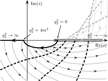
(b) $4m^{2}<q_{1}^{2}$

Figure 4: Movement of the trajectory of the anomalous threshold $s_{+}$ during the Wick rotation. The thick gray line on the real axis is the unitarity cut for $s>4m^{2}$. The solid line denotes the trajectory of $s_{+}$ for a fixed $q_{1}^{2}>0$: the anomalous threshold enters the physical sheet through the unitarity cut when $q_{2}^{2}$ increases. The dotted lines show the movement of $s_{+}$ when $q_{1}$ and $q_{2}$ are simultaneously Wick rotated: it retreats through the unitarity cut into the second Riemann sheet. The dashed lines show intermediate trajectories of $s_{+}$ during the Wick rotation. The part of the trajectories that lies on the second sheet is shown in light gray, the part on the physical sheet is black.

As a further check we have calculated numerically a simplified toy example that exhibits all relevant features discussed above. We consider

$$a_{\mu}^{\text{toy}}=(4\pi)^{4}\int\frac{d^{4}q_{1}}{(2\pi)^{4}}\int\frac{d^{4}q_{2}}{(2\pi)^{4}}\frac{m_{\mu}^{2}}{\big{(}q_{1}^{2}+i\epsilon\big{)}\big{(}q_{2}^{2}+i\epsilon\big{)}(s+i\epsilon)\big{(}s-m_{\mu}^{2}+i\epsilon\big{)}}\int_{0}^{1}dx\int_{0}^{1-x}dy\,\Delta(x,y)^{-1},$$ (4.33)

where

$$\Delta(x,y)=M_{\pi}^{2}-xys-x(1-x-y)q_{1}^{2}-y(1-x-y)q_{2}^{2}-i\epsilon.$$ (4.34)

The function defined by the last two integrals is proportional to the Feynman-parameter representation of the triangle loop function $C_{0}(s;q_{1}^{2},q_{2}^{2})$, while the remainder of $a_{\mu}^{\text{toy}}$ is chosen in as close analogy to the real HLbL integral as possible, including a sufficient number of propagators to make the integral converge. In the standard loop-integral approach the intricacies due to anomalous thresholds are automatically taken into account by the $i\epsilon$-prescription in (4.33) and (4.34), leading to the following Feynman-parameter representation

$$a_{\mu}^{\text{toy}} =-\int_{0}^{1}dx\int_{0}^{1-x}dy\int_{0}^{1}dx_{1}\int_{0}^{1-x_{1}}dx_{2}\int_{0}^{1}dx_{3}\frac{\log\Big{(}1+\frac{x_{2}}{x_{1}}\frac{m_{\mu}^{2}}{M_{\pi}^{2}}\Big{)}}{\Delta_{1}(x_{1},y)\Delta_{2}(x_{1},x_{2},x_{3},x,y)^{2}},$$

$$\Delta_{1}(x_{1},y) =1-x_{1}+x_{1}y(1-y),$$

$$\Delta_{2}(x_{1},x_{2},x_{3},x,y) =\big{(}1-x_{3}\big{)}\Delta_{1}(x_{1},y)+x_{3}\big{(}x_{2}+x_{1}x(1-x)\big{)}-x_{3}\frac{(x_{2}+x_{1}xy)^{2}}{\Delta_{1}(x_{1},y)}.$$ (4.35)

In analogy to the HLbL master formula (4.28) the Wick-rotated representation becomes (the $Q_{i}$ have been rescaled by $m_{\mu}$)

$$a_{\mu}^{\text{toy}} =-\frac{8}{\pi}\int_{0}^{\infty}dQ_{1}\int_{0}^{\infty}dQ_{2}\int_{-1}^{1}d\tau\frac{\sqrt{1-\tau^{2}}Q_{1}Q_{2}}{Q_{3}^{2}\big{(}1+Q_{3}^{2}\big{)}}\int_{0}^{1}dx\int_{0}^{1-x}dy\,\tilde{\Delta}(x,y)^{-1},$$

$$\tilde{\Delta}(x,y) =\frac{M_{\pi}^{2}}{m_{\mu}^{2}}+xyQ_{3}^{2}+x(1-x-y)Q_{1}^{2}+y(1-x-y)Q_{2}^{2}.$$ (4.36)

We checked numerically that indeed the representations (4.4) and (4.4) are identical. This confirms that the Wick rotation is permitted despite the occurrence of anomalous thresholds, all signs of which disappear in the Feynman parameterization as long as the $i\epsilon$-prescription is applied consistently. Similarly, the final result for the Wick rotation displays no remnants of the anomalous thresholds. As shown in Fig. 4, in this case the deeper reason can be traced back to the trajectory of the anomalous threshold during the Wick rotation towards the second sheet.

Finally, we note that the above discussion of the anomalous threshold of the triangle diagram is already sufficient for the full HLbL calculation. Box diagrams do not lead to further complications, since, in the master formula (4.23), the limit $k\to 0$ is taken before the Wick rotation of the loop momenta, hence the analytic structure of box diagrams is already reduced to the one of triangle diagrams.

5 Mandelstam representation

In the previous section, we have obtained a master formula (4.28) for the HLbL contribution to the anomalous magnetic moment of the muon, where the hadronic dynamics is parametrized in terms of the scalar functions $\Pi_{i}$. Since these functions are free of kinematic singularities and zeros, they are the quantities that should satisfy a Mandelstam representation [61]. We need to determine seven scalar functions that are not related to each other by crossing symmetry. Due to the complexity of the problem, we cannot obtain an exact solution for the scalar functions but have to rely on approximations. Our strategy is to order the contributions to the scalar functions by the mass of the intermediate states. The lightest intermediate states are expected to give the most important contribution, heavier states are suppressed by the higher threshold and smaller phase space. In this paper, we will consider the two lowest-lying contributions: one- and two-pion intermediate states in all channels, i.e. pion-pole and pion-box topologies. These two contributions can be described without any further approximation. Of course, pion-pole and pion-loop contributions have been considered before in various model calculations. The important point of the dispersive approach is that these contributions become unambiguously defined: the pion pole, with on-shell pion transition form factor, corresponds precisely to one-pion intermediate states, and the sQED pion loop dressed with pion vector form factors to two-pion intermediate states with pion-pole LHC. The explicit proof of these identifications will be presented in this section, based on a Mandelstam representation for the BTT scalar functions.

5.1 Derivation of the double-spectral representation

For the derivation of a Mandelstam representation of the scalar functions, we follow the discussion in [62]. We assume that the photon virtualities $q_{i}^{2}$ are fixed and small enough so that no anomalous thresholds are present. A parameter-free description of the HLbL tensor and therefore an unsubtracted dispersion relation is crucial. The behavior of the imaginary parts, which is determined by the asymptotics of the sub-processes, does indeed suggest that no subtractions are needed. Furthermore, even a quark-loop contribution to the HLbL tensor has an asymptotic behavior that requires no subtractions. Hence, for a generic scalar function $\Pi_{i}$, we write a fixed-$t$ dispersion relation without any subtractions:

$$\Pi_{i}^{t}(s,t,u) =c_{i}^{t}+\frac{\rho_{i;s}^{t}}{s-M_{\pi}^{2}}+\frac{\rho_{i;u}^{t}}{u-M_{\pi}^{2}}+\frac{1}{\pi}\int_{4M_{\pi}^{2}}^{\infty}ds^{\prime}\frac{\mathrm{Im}_{s}\Pi_{i}^{t}(s^{\prime},t,u^{\prime})}{s^{\prime}-s}+\frac{1}{\pi}\int_{4M_{\pi}^{2}}^{\infty}du^{\prime}\frac{\mathrm{Im}_{u}\Pi_{i}^{t}(s^{\prime},t,u^{\prime})}{u^{\prime}-u},$$ (5.1)

where $c_{i}^{t}$ is supposed to behave as $\lim\limits_{t\to 0}c_{i}^{t}=0$ and takes into account the $t$-channel pole. The imaginary parts are understood to be evaluated just above the corresponding cut. The primed variables fulfill

$$s^{\prime}+t+u^{\prime}=\Sigma:=\sum_{i=1}^{4}q_{i}^{2}.$$ (5.2)

If we continue the fixed-$t$ dispersion relation analytically in $t$, we have to replace the imaginary parts by the discontinuities, defined by

$$\begin{split}D_{i;s}^{t}(s^{\prime})&:=\frac{1}{2i}\left(\Pi_{i}^{t}(s^{\prime}+i\epsilon,t,u^{\prime})-\Pi_{i}^{t}(s^{\prime}-i\epsilon,t,u^{\prime})\right),\\ D_{i;u}^{t}(u^{\prime})&:=\frac{1}{2i}\left(\Pi_{i}^{t}(s^{\prime},t,u^{\prime}+i\epsilon)-\Pi_{i}^{t}(s^{\prime},t,u^{\prime}-i\epsilon)\right),\end{split}$$ (5.3)

hence

$$\Pi_{i}^{t}(s,t,u) =c_{i}^{t}+\frac{\rho_{i;s}^{t}}{s-M_{\pi}^{2}}+\frac{\rho_{i;u}^{t}}{u-M_{\pi}^{2}}+\frac{1}{\pi}\int_{4M_{\pi}^{2}}^{\infty}ds^{\prime}\frac{D_{i;s}^{t}(s^{\prime})}{s^{\prime}-s}+\frac{1}{\pi}\int_{4M_{\pi}^{2}}^{\infty}du^{\prime}\frac{D_{i;u}^{t}(u^{\prime})}{u^{\prime}-u}.$$ (5.4)

Both the discontinuities as well as the pole residues are determined by $s$- or $u$-channel unitarity, which also defines their analytic continuation in $t$. While $\rho^{t}_{i;s,u}$ are due to a one-pion intermediate state, $D_{i;s,u}^{t}$ are due to multi-particle intermediate states, see Fig. 5. We limit ourselves to two-pion intermediate states and neglect the contribution of heavier intermediate states to the discontinuities.

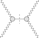
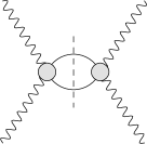
Figure 5: Intermediate states in the direct channel: pion pole and two-pion cut.

First, we study the pion-pole contribution by analyzing the unitarity relation:

$$\begin{split}\mathrm{Im}_{s}&\left(e^{4}(2\pi)^{4}\delta^{(4)}(q_{1}+q_{2}+q_{3}-q_{4})H_{\lambda_{1}\lambda_{2},\lambda_{3}\lambda_{4}}\right)\\ &=\sum_{n}\frac{1}{2S_{n}}\left(\prod_{i=1}^{n}\int\widetilde{dp_{i}}\right)\langle\gamma^{*}(-q_{3},\lambda_{3})\gamma^{*}(q_{4},\lambda_{4})|n;\{p_{i}\}\rangle^{*}\langle\gamma^{*}(q_{1},\lambda_{1})\gamma^{*}(q_{2},\lambda_{2})|n;\{p_{i}\}\rangle,\end{split}$$ (5.5)

where $S_{n}$ is the symmetry factor of the intermediate state $|n\rangle$. We consider now only the $\pi^{0}$ intermediate state in the sum:

$$\begin{split}\mathrm{Im}_{s}^{\pi}&\left(e^{4}(2\pi)^{4}\delta^{(4)}(q_{1}+q_{2}+q_{3}-q_{4})H_{\lambda_{1}\lambda_{2},\lambda_{3}\lambda_{4}}\right)\\ &=\frac{1}{2}\int\widetilde{dp}\;\langle\gamma^{*}(-q_{3},\lambda_{3})\gamma^{*}(q_{4},\lambda_{4})|\pi^{0}(p)\rangle^{*}\langle\gamma^{*}(q_{1},\lambda_{1})\gamma^{*}(q_{2},\lambda_{2})|\pi^{0}(p)\rangle.\end{split}$$ (5.6)

After reducing the matrix elements and using the definition of the pion transition form factor

$$i\int d^{4}x\;e^{iq\cdot x}\langle 0|T\{j^{\mu}_{\mathrm{em}}(x)j^{\nu}_{\mathrm{em}}(0)\}|\pi^{0}(p)\rangle=\epsilon^{\mu\nu\alpha\beta}q_{\alpha}p_{\beta}\mathcal{F}_{\pi^{0}\gamma^{*}\gamma^{*}}\big{(}q^{2},(q-p)^{2}\big{)},$$ (5.7)

we find

$$\begin{split}\mathrm{Im}_{s}^{\pi}\Pi^{\mu\nu\lambda\sigma}&=-\frac{1}{2}\begin{aligned} &\int\widetilde{dp}\;(2\pi)^{4}\delta^{(4)}(q_{1}+q_{2}-p)\epsilon^{\mu\nu\alpha\beta}\epsilon^{\lambda\sigma\gamma\delta}{q_{1}}_{\alpha}{q_{2}}_{\beta}{q_{3}}_{\gamma}{q_{4}}_{\delta}\\ &\quad\times\mathcal{F}_{\pi^{0}\gamma^{*}\gamma^{*}}\big{(}q_{1}^{2},q_{2}^{2}\big{)}\mathcal{F}_{\pi^{0}\gamma^{*}\gamma^{*}}\big{(}q_{3}^{2},q_{4}^{2}\big{)}\end{aligned}\\ &=-\pi\delta(s-M_{\pi}^{2})\epsilon^{\mu\nu\alpha\beta}\epsilon^{\lambda\sigma\gamma\delta}{q_{1}}_{\alpha}{q_{2}}_{\beta}{q_{3}}_{\gamma}{q_{4}}_{\delta}\mathcal{F}_{\pi^{0}\gamma^{*}\gamma^{*}}\big{(}q_{1}^{2},q_{2}^{2}\big{)}\mathcal{F}_{\pi^{0}\gamma^{*}\gamma^{*}}\big{(}q_{3}^{2},q_{4}^{2}\big{)}.\end{split}$$ (5.8)

By projecting onto the scalar functions $\Pi_{i}$, this leads to

$$\rho_{i;s}^{t} =\left\{\begin{matrix}\mathcal{F}_{\pi^{0}\gamma^{*}\gamma^{*}}\big{(}q_{1}^{2},q_{2}^{2}\big{)}\mathcal{F}_{\pi^{0}\gamma^{*}\gamma^{*}}\big{(}q_{3}^{2},q_{4}^{2}\big{)}&i=1,\\ 0&i\neq 1,\end{matrix}\right.$$ (5.9)

and, analogously,

$$\rho_{i;u}^{t} =\left\{\begin{matrix}\mathcal{F}_{\pi^{0}\gamma^{*}\gamma^{*}}\big{(}q_{1}^{2},q_{4}^{2}\big{)}\mathcal{F}_{\pi^{0}\gamma^{*}\gamma^{*}}\big{(}q_{2}^{2},q_{3}^{2}\big{)}&i=3,\\ 0&i\neq 3.\end{matrix}\right.$$ (5.10)

In order to identify the discontinuities, we project the unitarity relation selecting two-pion intermediate states:

$$\begin{split}&\mathrm{Im}_{s}^{\pi\pi}\left(e^{4}(2\pi)^{4}\delta^{(4)}(q_{1}+q_{2}+q_{3}-q_{4})H_{\lambda_{1}\lambda_{2},\lambda_{3}\lambda_{4}}\right)\\ &=\frac{1}{2}\int\widetilde{dp}_{1}\widetilde{dp}_{2}\langle\pi^{+}(p_{1})\pi^{-}(p_{2})|\gamma^{*}(-q_{3},\lambda_{3})\gamma^{*}(q_{4},\lambda_{4})\rangle^{*}\langle\pi^{+}(p_{1})\pi^{-}(p_{2})|\gamma^{*}(q_{1},\lambda_{1})\gamma^{*}(q_{2},\lambda_{2})\rangle\\ &\quad+\frac{1}{4}\int\widetilde{dp}_{1}\widetilde{dp}_{2}\langle\pi^{0}(p_{1})\pi^{0}(p_{2})|\gamma^{*}(-q_{3},\lambda_{3})\gamma^{*}(q_{4},\lambda_{4})\rangle^{*}\langle\pi^{0}(p_{1})\pi^{0}(p_{2})|\gamma^{*}(q_{1},\lambda_{1})\gamma^{*}(q_{2},\lambda_{2})\rangle,\end{split}$$ (5.11)

hence

$$\mathrm{Im}_{s}^{\pi\pi}\Pi^{\mu\nu\lambda\sigma} =\frac{1}{32\pi^{2}}\frac{\sigma_{\pi}(s)}{2}\int d\Omega_{s}^{\prime\prime}\begin{aligned} &\bigg{(}W_{+-}^{\mu\nu}(p_{1},p_{2},q_{1}){W_{+-}^{\lambda\sigma}}^{*}(p_{1},p_{2},-q_{3})\\ &+\frac{1}{2}W_{00}^{\mu\nu}(p_{1},p_{2},q_{1}){W_{00}^{\lambda\sigma}}^{*}(p_{1},p_{2},-q_{3})\bigg{)},\end{aligned}$$

where the subscripts $\{+-,00\}$ denote the pion charges. The analytic continuation of the unitarity relation can be obtained if the $\gamma^{*}\gamma^{*}\to\pi\pi$ matrix element $W^{\mu\nu}$ is expressed in terms of the fixed-$s$ dispersion relation (2.42) for its scalar functions:

$$\begin{split}W_{+-}^{\mu\nu}&=\sum_{i=1}^{5}T^{\mu\nu}_{i}\begin{aligned} &\Bigg{(}\frac{\hat{\rho}_{i;t}^{s;+-}(s)}{t-M_{\pi}^{2}}+\frac{\hat{\rho}_{i;u}^{s;+-}(s)}{u-M_{\pi}^{2}}+\frac{1}{\pi}\int_{4M_{\pi}^{2}}^{\infty}dt_{1}\frac{\hat{D}_{i;t}^{s;+-}(t_{1};s)}{t_{1}-t}+\frac{1}{\pi}\int_{4M_{\pi}^{2}}^{\infty}du_{1}\frac{\hat{D}_{i;u}^{s;+-}(u_{1};s)}{u_{1}-u}\Bigg{)},\end{aligned}\\ W_{00}^{\mu\nu}&=\sum_{i=1}^{5}T^{\mu\nu}_{i}\begin{aligned} &\Bigg{(}\frac{1}{\pi}\int_{4M_{\pi}^{2}}^{\infty}dt_{1}\frac{\hat{D}_{i;t}^{s;00}(t_{1};s)}{t_{1}-t}+\frac{1}{\pi}\int_{4M_{\pi}^{2}}^{\infty}du_{1}\frac{\hat{D}_{i;u}^{s;00}(u_{1};s)}{u_{1}-u}\Bigg{)}.\end{aligned}\end{split}$$ (5.13)

Note that $W_{00}^{\mu\nu}$ does not contain any pole terms because the photon does not couple to two neutral pions due to angular momentum conservation and Bose symmetry.

If we pick the contribution of the pole terms on both sides of the cut, we single out box topologies:

$$\mathrm{Im}_{s}^{\pi\pi}\Pi^{\mu\nu\lambda\sigma}\Big{|}_{\mathrm{box}} =\frac{1}{32\pi^{2}}\frac{\sigma_{\pi}(s)}{2}\int d\Omega_{s}^{\prime\prime}\sum_{i,j=1,4}T^{\mu\nu}_{i}T^{\lambda\sigma}_{j}\Bigg{(}\frac{\hat{\rho}_{i;t}^{s;+-}(s)}{t^{\prime}-M_{\pi}^{2}}+\frac{\hat{\rho}_{i;u}^{s;+-}(s)}{u^{\prime}-M_{\pi}^{2}}\Bigg{)}\Bigg{(}\frac{\hat{\rho}_{j;t}^{s;+-}(s)}{t^{\prime\prime}-M_{\pi}^{2}}+\frac{\hat{\rho}_{j;u}^{s;+-}(s)}{u^{\prime\prime}-M_{\pi}^{2}}\Bigg{)}^{*},$$ (5.14)

where the primed variables belong to the sub-process on the left-hand side and the double-primed variables to the sub-process on the right-hand side of the cut.

We could now apply a tensor reduction to obtain phase-space integrals for the reduced scalar quantities. The projection on the scalar functions $\Pi_{i}$ would allow us to identify the discontinuities $D_{i;s}^{t}$ due to box structures. The reduced scalar integrals could then be transformed into another dispersive integral. Together with the dispersion integral $ds^{\prime}$ of the primary cut, this produces the double-spectral representation. The case of the simplest scalar phase-space integral is explained in [33].

Unfortunately, the tensor reduction is enormously complex because it involves the inversion of a $138\times 138$ square matrix. We will therefore follow a different strategy for the box topologies. We note that the non-zero pole residues $\hat{\rho}_{i;t,u}^{s;+-}$ contain two electromagnetic pion form factors for the off-shell photons. These form factors can be factored out and multiply then the discontinuity that would be obtained by applying Cutkosky’s rules [63] to the sQED pion loop calculation. This becomes clear from the relation between the pole terms and the sQED Born terms as discussed Sect. 2.6. Therefore, the box contribution is nothing else but the sQED contribution multiplied by a vector form factor $F_{\pi}^{V}(q_{i}^{2})$ for each of the off-shell photons. As in the case of the sub-process, the difference between unitarity diagrams and Feynman diagrams is absolutely crucial: the sQED contribution consists of boxes, triangles, and bulb Feynman diagrams, but corresponds to the pure box topology in terms of unitarity. In Sect. 5.3, we will prove that this identification is correct and unique.

Finally, there are the contributions with discontinuities either in one or in both of the sub-processes. They contain for example resonance contributions in the sub-process, but also two-pion rescattering effects in the direct channel.

5.2 Symmetrization and classification into topologies

In the previous subsection, we have explained how the double-spectral representation can be derived from a fixed-$t$ dispersion relation by taking the analytic continuation in $t$, which is defined by the unitarity relation. In the $s$-channel unitarity relation, a fixed-$s$ dispersion relation of the sub-process is inserted (in the unitarity relation for the $u$-channel contribution, the variable $u$ is kept fixed, which, however, plays again the role of $s$ in the sub-process). Of course, one could have started with a fixed-$u$ or fixed-$s$ dispersion relation in the first place. The requirement that this lead to the same result allows us to identify a symmetric representation, which treats the Mandelstam variables on an equal footing and therefore implements crossing symmetry. In this symmetric representation, we classify the different contributions in terms of topologies. Note that in the case of HLbL, we get the two other possibilities (i.e. taking fixed-$u$ and fixed-$s$ dispersion relations as the starting point) for free, because we consider a totally crossing symmetric process.

If we compare the three different representations of unsubtracted dispersion relations (5.4), we immediately see that the contributions in one representation are either contained explicitly in the other representations, can be understood as part of the respective constant $c_{i}^{t}$, or correspond to a contribution of neglected higher intermediate states, as we are now going to discuss.

5.2.1 Pion-pole contribution

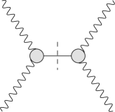
Figure 6: Unitarity diagram representing the pion-pole contribution in one channel.

First, we consider the pion-pole topology (see Fig. 6). The fixed-$t$ dispersion relation contains the poles in the $s$- and $u$-channel explicitly. Analogously, the fixed-$s$ (fixed-$u$) dispersion relation contains the poles in the $t$- and $u$-channel ($s$- and $t$-channel). The $t$-channel pole contribution, which is not explicit in the fixed-$t$ representation, can be identified with $c_{i}^{t}$ as it vanishes in the limit $t\to\infty$. Hence, the total pion-pole contribution is just given by

$$\Pi_{i}^{\pi^{0}\text{-pole}}(s,t,u) =\frac{\rho_{i;s}}{s-M_{\pi}^{2}}+\frac{\rho_{i;t}}{t-M_{\pi}^{2}}+\frac{\rho_{i;u}}{u-M_{\pi}^{2}},$$ (5.15)

where the pole residues are products of pion transition form factors:

$$\begin{split}\rho_{i,s}&=\delta_{i1}\;\mathcal{F}_{\pi^{0}\gamma^{*}\gamma^{*}}\big{(}q_{1}^{2},q_{2}^{2}\big{)}\mathcal{F}_{\pi^{0}\gamma^{*}\gamma^{*}}\big{(}q_{3}^{2},q_{4}^{2}\big{)},\\ \rho_{i,t}&=\delta_{i2}\;\mathcal{F}_{\pi^{0}\gamma^{*}\gamma^{*}}\big{(}q_{1}^{2},q_{3}^{2}\big{)}\mathcal{F}_{\pi^{0}\gamma^{*}\gamma^{*}}\big{(}q_{2}^{2},q_{4}^{2}\big{)},\\ \rho_{i,u}&=\delta_{i3}\;\mathcal{F}_{\pi^{0}\gamma^{*}\gamma^{*}}\big{(}q_{1}^{2},q_{4}^{2}\big{)}\mathcal{F}_{\pi^{0}\gamma^{*}\gamma^{*}}\big{(}q_{2}^{2},q_{3}^{2}\big{)},\\ \end{split}$$ (5.16)

where $\delta_{ij}$ is the Kronecker delta.

Since the Lorentz structures of the usual pion-pole contribution, see e.g. [19], coincide with the first three BTT structures, this proves that in a dispersive approach the pion pole is unambiguously defined as given in [26] (and already in [19]), in particular with the transition form factor defined for an on-shell pion.

5.2.2 Box contribution

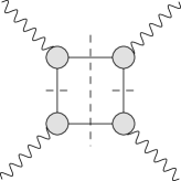
(a)

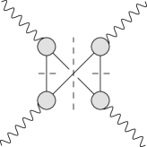
(b)

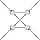
(c)

Figure 7: Unitarity diagrams representing the box contributions.

For the contribution of box topologies (see Fig. 7), Mandelstam diagrams prove very useful for the discussion of double-spectral regions. In Fig. 8, such a diagram is shown for the case $q_{i}^{2}=0.5M_{\pi}^{2}$. A dashed line indicates a line of fixed $t$, used for writing the fixed-$t$ dispersion relation. The two cuts are highlighted in gray. The discontinuities along these cuts can be written again as a dispersive integral over double-spectral functions. The three regions of non-vanishing double-spectral functions are labeled in Fig. 8 by $\rho_{st}$, $\rho_{su}$, and $\rho_{tu}$.

The $s$-channel cut receives contributions from the double-spectral regions $\rho_{st}$ and $\rho_{su}$, according to the unitarity diagrams 7(a) and 7(b), where first the vertical cut, then the horizontal cut is applied. The $u$-channel cut receives contributions again from $\rho_{su}$ and from $\rho_{tu}$, according to the unitarity diagrams 7(b) and 7(c). In diagram 7(b), the horizontal cut is now applied first.

Hence, the fixed-$t$ dispersion relation leads to a priori four double-spectral integrals: one for each of the regions $\rho_{st}$ and $\rho_{tu}$ and two for the region $\rho_{su}$. However, it turns out that the sum of the two double-spectral integrals for the region $\rho_{su}$ equals the crossed version of one of the other double-spectral integrals. This is illustrated for the example of a simple scalar box diagram in App. G.3. Therefore, the box contributions constructed from a fixed-$t$ dispersion relation are already crossing symmetric and identical to the box contributions that are obtained from a fixed-$s$ or fixed-$u$ dispersion relation.

This discussion already anticipates the idea of the uniqueness proof in Sect. 5.3: isolating the pion-pole contribution to the LHC in $\pi\pi$ intermediate states, the double-spectral functions become identical to the ones of the box diagrams in the sQED loop calculation. What needs to be shown is that the Lorentz structures in the BTT set not only produce the right Lorentz structures for the sQED box diagrams, but also that the triangle- and bulb-type sQED diagrams are correctly reproduced. Moreover, this identification has to be proven for the full set of BTT functions, including those which cannot immediately be identified with basis functions due to the occurrence of the Tarrach amplitudes.

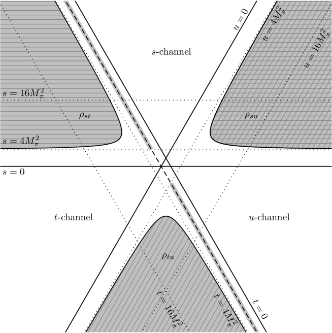
Figure 8: Mandelstam diagram for HLbL scattering for the case $q_{i}^{2}=0.5M_{\pi}^{2}$ with double-spectral regions for box topologies. The dashed line marks a line of fixed $t$ with its $s$- and $u$-channel cuts highlighted in gray.

5.2.3 Higher intermediate states

Topologies where we replace either one or both of the pion poles in the sub-process by a multi-particle cut are the last contribution with a two-pion intermediate state in the direct channel. Such contributions could be captured in several ways, either relying on a partial-wave picture or approximating the multi-pion states by an effective resonance description. While the case of $S$-waves was already discussed in [26], the BTT formulation facilitates the generalization to $D$-waves, since the technical complications related to angular averages and kinematic singularities, the latter requiring the introduction of off-diagonal kernels, are avoided. The application to rescattering effects will be presented in a forthcoming publication.

5.3 Uniqueness of the box topologies

In this subsection, we will prove that the box topologies are equal to the FsQED contribution (sQED multiplied by pion vector form factors) and that this contribution is unique. The proof is based on the Mandelstam representation and consists of two arguments:

• the double-spectral densities of box topologies and FsQED agree,

• both representations fulfill an unsubtracted Mandelstam representation.

The argument for the first point is the following: in the case of the box topologies, the discontinuities are defined by the unitarity relation as phase-space integrals of products of two pure pole contributions for $\gamma^{*}\gamma^{*}\to\pi\pi$. In the case of FsQED, the discontinuities are most easily found by applying Cutkosky’s rules [63], i.e. by cutting the loop diagrams. We see immediately that the discontinuities in FsQED are phase-space integrals of products of two Born terms for $\gamma^{*}\gamma^{*}\to\pi\pi$. In Sect. 2.6, we have already shown that the Born contribution is the same as the pure pole, hence the discontinuities (and therefore also the double-spectral densities) of the box topologies and FsQED are equal.

To complete the proof it remains to be shown that the scalar functions in FsQED fulfill a Mandelstam representation (the scalar functions of the box topologies are defined by the Mandelstam representation). Apart from the first six scalar functions $\Pi_{1},\ldots,\Pi_{6}$, which are unaffected by the Tarrach amplitudes, the scalar BTT functions $\Pi_{i}$ are defined only up to the ambiguity (3.22), so that we cannot compare the representations for these functions immediately. Therefore, we will derive the double-spectral representation of the basis functions $\tilde{\Pi}_{i}$ that is implied by an unsubtracted Mandelstam representation for the scalar functions $\Pi_{i}$ and show that the FsQED basis functions fulfill a double-spectral representation of this form. This will then complete the proof of the uniqueness and the equality of the box topologies and the FsQED contribution.

First, we calculate the fully off-shell sQED loop contribution. It consists of six box diagrams, twelve triangles, and three bulb diagrams:

$$ie^{4}\Pi_{\mathrm{sQED}}^{\mu\nu\lambda\sigma}=3\times\begin{minipage}{42.67912pt} \includegraphics[height=42.67912pt]{images/sQED_Bulb} \end{minipage}+12\times\begin{minipage}{42.67912pt} \includegraphics[height=42.67912pt]{images/sQED_Triangle} \end{minipage}+6\times\begin{minipage}{42.67912pt} \includegraphics[height=42.67912pt]{images/sQED_Box} \end{minipage}.$$ (5.17)

The three bulb diagrams are given by

$$3\times\begin{minipage}{42.67912pt} \includegraphics[height=42.67912pt]{images/sQED_Bulb} \end{minipage}=4ie^{4}\Big{(}g^{\mu\nu}g^{\lambda\sigma}B_{0}(s,M_{\pi}^{2},M_{\pi}^{2})+g^{\mu\lambda}g^{\nu\sigma}B_{0}(t,M_{\pi}^{2},M_{\pi}^{2})+g^{\mu\sigma}g^{\nu\lambda}B_{0}(u,M_{\pi}^{2},M_{\pi}^{2})\Big{)},$$ (5.18)

where the scalar loop function $B_{0}$ is defined in (G.1). One of the twelve triangle diagrams can be represented as

$$=4ie^{4}g^{\lambda\sigma}\begin{aligned} &\bigg{(}\frac{1}{2}q_{1}^{\mu}q_{2}^{\nu}C_{0}(q_{1}^{2},s,q_{2}^{2},M_{\pi}^{2},M_{\pi}^{2},M_{\pi}^{2})-q_{1}^{\mu}\left(q_{1}^{\nu}-q_{2}^{\nu}\right)C_{1}(q_{1}^{2},s,q_{2}^{2},M_{\pi}^{2},M_{\pi}^{2},M_{\pi}^{2})\\ &+q_{2}^{\nu}\left(q_{1}^{\mu}-q_{2}^{\mu}\right)C_{2}(q_{1}^{2},s,q_{2}^{2},M_{\pi}^{2},M_{\pi}^{2},M_{\pi}^{2})\\ &-2g^{\mu\nu}C_{00}(q_{1}^{2},s,q_{2}^{2},M_{\pi}^{2},M_{\pi}^{2},M_{\pi}^{2})+2\left(q_{1}^{\nu}q_{2}^{\mu}+q_{1}^{\mu}q_{2}^{\nu}\right)C_{12}(q_{1}^{2},s,q_{2}^{2},M_{\pi}^{2},M_{\pi}^{2},M_{\pi}^{2})\\ &-2q_{1}^{\mu}q_{1}^{\nu}C_{11}(q_{1}^{2},s,q_{2}^{2},M_{\pi}^{2},M_{\pi}^{2},M_{\pi}^{2})-2q_{2}^{\mu}q_{2}^{\nu}C_{22}(q_{1}^{2},s,q_{2}^{2},M_{\pi}^{2},M_{\pi}^{2},M_{\pi}^{2})\bigg{)},\end{aligned}$$

where the scalar loop function $C_{0}$ is defined in (G.4). For the tensor coefficient functions $C_{i}$, $C_{ij}$, we use the convention of [64] up to a normalization factor: $16\pi^{2}C_{0}=C_{0}^{\text{\cite[cite]{[\@@bibref{Number}{Denner1993}{}{}]}}}$ etc. The remaining eleven triangles follow by crossing the external momenta. Similarly, the fully off-shell formula for the box diagrams can also be expressed in terms of the scalar four-point function $D_{0}$ and the tensor coefficient functions $D_{i}$, $D_{ij}$, $D_{ijk}$, $D_{ijkl}$, but the result is rather long and need not be reproduced here.

In this way, we obtain a representation in terms of scalar loop functions $B_{0}$, $C_{0}$, $D_{0}$, and the pertinent tensor coefficient functions. Next, we project this expression onto the HLbL tensor basis (3.18), see App. C, in order to identify the sQED contribution to the basis functions $\tilde{\Pi}_{i}$. Using FeynCalc [65], we perform a Passarino–Veltman reduction [66, 67] of the tensor coefficient functions, so that the basis functions are given by linear combinations of the scalar loop functions:

$$\begin{split}\tilde{\Pi}_{i}^{\mathrm{sQED}}&=p_{i}+a_{i}A_{0}(M_{\pi}^{2})\\ &\quad+b_{i}^{1}B_{0}(q_{1}^{2},M_{\pi}^{2},M_{\pi}^{2})+b_{i}^{2}B_{0}(q_{2}^{2},M_{\pi}^{2},M_{\pi}^{2})+b_{i}^{3}B_{0}(q_{3}^{2},M_{\pi}^{2},M_{\pi}^{2})+b_{i}^{4}B_{0}(q_{4}^{2},M_{\pi}^{2},M_{\pi}^{2})\\ &\quad+b_{i}^{s}B_{0}(s,M_{\pi}^{2},M_{\pi}^{2})+b_{i}^{t}B_{0}(t,M_{\pi}^{2},M_{\pi}^{2})+b_{i}^{u}B_{0}(u,M_{\pi}^{2},M_{\pi}^{2})\\ &\quad+c_{i}^{12}C_{0}(q_{1}^{2},q_{2}^{2},s,M_{\pi}^{2},M_{\pi}^{2},M_{\pi}^{2})+c_{i}^{13}C_{0}(q_{1}^{2},q_{3}^{2},t,M_{\pi}^{2},M_{\pi}^{2},M_{\pi}^{2})+c_{i}^{14}C_{0}(q_{1}^{2},q_{4}^{2},u,M_{\pi}^{2},M_{\pi}^{2},M_{\pi}^{2})\\ &\quad+c_{i}^{34}C_{0}(q_{3}^{2},q_{4}^{2},s,M_{\pi}^{2},M_{\pi}^{2},M_{\pi}^{2})+c_{i}^{24}C_{0}(q_{2}^{2},q_{4}^{2},t,M_{\pi}^{2},M_{\pi}^{2},M_{\pi}^{2})+c_{i}^{23}C_{0}(q_{2}^{2},q_{3}^{2},u,M_{\pi}^{2},M_{\pi}^{2},M_{\pi}^{2})\\ &\quad+d_{i}^{st}D_{0}(q_{1}^{2},q_{2}^{2},q_{4}^{2},q_{3}^{2},s,t,M_{\pi}^{2},M_{\pi}^{2},M_{\pi}^{2},M_{\pi}^{2})\\ &\quad+d_{i}^{su}D_{0}(q_{1}^{2},q_{2}^{2},q_{3}^{2},q_{4}^{2},s,u,M_{\pi}^{2},M_{\pi}^{2},M_{\pi}^{2},M_{\pi}^{2})\\ &\quad+d_{i}^{tu}D_{0}(q_{1}^{2},q_{3}^{2},q_{2}^{2},q_{4}^{2},t,u,M_{\pi}^{2},M_{\pi}^{2},M_{\pi}^{2},M_{\pi}^{2}),\end{split}$$ (5.20)

where the coefficients $p_{i}$, $a_{i}$, $b_{i}^{j}$, $c_{i}^{j}$, $d_{i}^{j}$ are meromorphic functions of the virtualities $q_{i}^{2}$ and the Mandelstam variables $s$, $t$, $u$. The Passarino–Veltman reduction results unfortunately in extremely long expressions for the coefficients, which, in addition, contain many kinematic singularities. However, at the kinematic points of these singularities the scalar loop functions fulfill linear relations which cancel most of the singularities. By evaluating the expressions for the functions $\tilde{\Pi}_{i}^{\mathrm{sQED}}$ numerically, we have checked that the only surviving kinematic singularities are exactly the ones required by the projection of the 54 scalar functions $\Pi_{i}$ onto the basis (B.2).

As already mentioned, the verification of the Mandelstam representation is simplest for the functions $\Pi_{1},\ldots,\Pi_{6}$, because they are identical to the basis functions $\tilde{\Pi}_{1},\ldots,\tilde{\Pi}_{6}$, i.e. their projection does not involve kinematic singularities. We have to show that these functions fulfill a Mandelstam representation of the form (suppressing the $i\epsilon$)

$$\begin{split}\Pi_{i}^{\mathrm{sQED}}(s,t,u)&=\frac{1}{\pi^{2}}\int_{4M_{\pi}^{2}}^{\infty}ds^{\prime}\int_{t^{+}(s^{\prime})}^{\infty}dt^{\prime}\frac{\rho_{i;st}^{\mathrm{sQED}}(s^{\prime},t^{\prime})}{(s^{\prime}-s)(t^{\prime}-t)}\\ &+\frac{1}{\pi^{2}}\int_{4M_{\pi}^{2}}^{\infty}ds^{\prime}\int_{u^{+}(s^{\prime})}^{\infty}du^{\prime}\frac{\rho_{i;su}^{\mathrm{sQED}}(s^{\prime},u^{\prime})}{(s^{\prime}-s)(u^{\prime}-u)}\\ &+\frac{1}{\pi^{2}}\int_{4M_{\pi}^{2}}^{\infty}dt^{\prime}\int_{u^{+}(t^{\prime})}^{\infty}du^{\prime}\frac{\rho_{i;tu}^{\mathrm{sQED}}(t^{\prime},u^{\prime})}{(t^{\prime}-t)(u^{\prime}-u)},\end{split}$$ (5.21)

where the borders of the double-spectral regions $t^{+},u^{+}$ are defined in (G.12).

As the scalar four-point functions $D_{0}$ are the only ones in (5.20) with a double-spectral region, we can immediately identify the double-spectral densities:

$$\left.\begin{aligned} \rho_{i;st}^{\mathrm{sQED}}(s,t)&=d_{i}^{st}(s,t)\rho_{0}(s,t;q_{1}^{2},q_{2}^{2},q_{4}^{2},q_{3}^{2}),\\ \rho_{i;su}^{\mathrm{sQED}}(s,u)&=d_{i}^{su}(s,u)\rho_{0}(s,u;q_{1}^{2},q_{2}^{2},q_{3}^{2},q_{4}^{2}),\\ \rho_{i;tu}^{\mathrm{sQED}}(t,u)&=d_{i}^{tu}(t,u)\rho_{0}(t,u;q_{1}^{2},q_{3}^{2},q_{2}^{2},q_{4}^{2})\end{aligned}\quad\right\}\quad i=\{1,\ldots,6\},$$

where $\rho_{0}$ is the double-spectral density of the $D_{0}$ scalar loop function, defined in (G.15). By evaluating numerically the double-spectral integrals (5.21) at some random kinematic points below the appearance of anomalous thresholds, we have checked that the Mandelstam representation for the functions $\Pi_{1}^{\mathrm{sQED}},\ldots,\Pi_{6}^{\mathrm{sQED}}$ indeed agrees with the expression in terms of scalar loop functions (5.20). Even though showing the identity of the two expressions algebraically would have been desirable, already the sheer size of these expressions has prevented an analytic comparison. However, the numerical check does not leave any room open for differences.

This result implies that the double-spectral densities of the sQED box diagrams (5.3) have the correct form that, when inserted into the Mandelstam representation, the non-residue pieces can be separated in such a way that all triangle and bulb loop functions in (5.20) are reproduced with the correct coefficients. The explicit verification of this property is the crucial point in the argument. Since the double-spectral densities of box topologies and FsQED agree, this proves the claim for $i=1,\ldots,6$.

The remaining basis functions exhibit kinematic singularities. In order to work out their double-dispersive representation, we can limit ourselves to the seven remaining representatives of (3.19). All other basis functions are related by crossing symmetry (B.2).

We write the basis functions of interest as

$$-4q_{3}\cdot q_{4}\tilde{\Pi}_{7} =2(s-s_{b})\Pi_{7}-(u-u_{a})(t-t_{b})\Pi_{31},$$

$$-2q_{3}\cdot q_{4}\tilde{\Pi}_{9} =(s-s_{b})\Pi_{9}+(u-u_{b})\Pi_{22},$$

$$-4q_{3}\cdot q_{4}\tilde{\Pi}_{19} =2(s-s_{b})\Pi_{19}+(u-u_{a})(u-u_{b})\Pi_{31},$$

$$-4q_{1}\cdot q_{2}q_{3}\cdot q_{4}\tilde{\Pi}_{21} =(s-s_{a})(s-s_{b})\Pi_{21}-(u-u_{a})(u-u_{b})\Pi_{22},$$

$$2q_{1}\cdot q_{2}\tilde{\Pi}_{36} =(s-s_{a})\Pi_{43}-(u-u_{b})\Pi_{37},$$

$$-2q_{3}\cdot q_{4}\tilde{\Pi}_{39} =(s-s_{b})\Pi_{49}-(s-s_{a})\Pi_{54},$$

$$-2q_{3}\cdot q_{4}\tilde{\Pi}_{40} =(s-s_{b})\Pi_{50}-(t-t_{b})\Pi_{54},$$

where $s_{a}:=q_{1}^{2}+q_{2}^{2}$, $s_{b}:=q_{3}^{2}+q_{4}^{2}$, $u_{a}:=q_{2}^{2}+q_{3}^{2}$, $u_{b}:=q_{1}^{2}+q_{4}^{2}$, $t_{b}:=q_{2}^{2}+q_{4}^{2}$. Next, we introduce subtractions for the scalar functions $\Pi_{i}$: each function is subtracted once or twice at the subtraction point that appears in the coefficient of the other function $\Pi_{i}$ in the above linear combinations. For instance, in the equation for $\tilde{\Pi}_{9}$, we subtract $\Pi_{9}$ at $u=u_{b}$ and $\Pi_{22}$ at $s=s_{b}$. This leads to representations of the basis functions $\tilde{\Pi}_{i}$ where both double-spectral contributions are multiplied by a common prefactor (e.g. $(s-s_{b})(u-u_{b})$ in the case of $\tilde{\Pi}_{9}$), while only the subtraction terms, which are single-dispersion integrals, have different prefactors. The results for these double-spectral representations of the basis functions $\tilde{\Pi}_{i}$ are given in (F.1) and (F.1) in App. F.1.

The important point is that in these double-spectral representations both the discontinuities of the single-dispersion integrals and the combined double-spectral densities $\tilde{\rho}_{i}$ are unambiguously defined. We do not attempt to split the double-spectral densities into two contributions from the $\Pi_{i}$: this splitting involves exactly the ambiguity (3.22). For the sQED contribution, the discontinuities and double-spectral densities can be extracted from the loop representation of the basis functions (5.20) as follows:

• The discontinuities are extracted by taking the appropriate limit of the basis functions $\tilde{\Pi}_{i}$. For instance, the discontinuity of the subtraction term of $\Pi_{9}$ is obtained by considering the limit $\lim\limits_{u\to u_{b}}(-2q_{3}\cdot q_{4}\tilde{\Pi}_{9})$.

• The combined double-spectral densities $\tilde{\rho}_{i}$ are (up to a kinematic factor) just the double-spectral densities of the basis functions $\tilde{\Pi}_{i}$. Therefore, they can be obtained again from the coefficients of the $D_{0}$ functions in the loop representation, in analogy to the case of $\tilde{\Pi}_{1},\ldots,\tilde{\Pi}_{6}$.

After having identified all the discontinuities and double-spectral densities in (F.1) and (F.1), we have checked numerically for random kinematic points (below the appearance of anomalous thresholds) that the dispersive representations of the functions $\tilde{\Pi}_{i}$ agrees with the loop representation. It turns out that $\tilde{\Pi}_{39}^{\mathrm{sQED}}=\tilde{\Pi}_{40}^{\mathrm{sQED}}=0$, hence we can set

$$\Pi_{49}^{\mathrm{sQED}}=\ldots=\Pi_{54}^{\mathrm{sQED}}=0,$$ (5.24)

which also fixes the redundancy (3.23).

This completes our proof of the uniqueness of the pion-box contribution. Cutkosky’s rules tell us that the discontinuities of the FsQED contribution are the same as the ones of the pion-box topologies in the sense of unitarity. The FsQED contribution fulfills the same double-spectral representation as the pure pion-box topologies. Therefore, the two representations are the same. Unitarity and Mandelstam analyticity define the pion-box contribution, i.e. $\pi\pi$ intermediate states with a pion-pole LHC, in a unique way.

Finally, we stress that these calculations also provide a strong test of the Lorentz decomposition (3.13). Apart from the function $\Pi_{49}$, which does not receive a contribution from the pion loop, all scalar functions have been shown to be free of kinematics, so that the sQED pion-loop amplitude behaves exactly as expected from the general BTT formalism.

5.4 Contribution to $\boldsymbol{(g-2)_{\mu}}$

In this subsection, we insert our dispersive representation of the scalar functions into the master formula (4.28) to obtain the contribution to $a_{\mu}$.

5.4.1 Pion-pole contribution

With (5.15) and using the master formula (4.28), we recover the well-known result for the pion-pole contribution to $a_{\mu}$ [19]:

$$\begin{split}a_{\mu}^{\pi^{0}\text{-pole}}&=\frac{2\alpha^{3}}{3\pi^{2}}\int_{0}^{\infty}dQ_{1}\int_{0}^{\infty}dQ_{2}\int_{-1}^{1}d\tau\sqrt{1-\tau^{2}}Q_{1}^{3}Q_{2}^{3}\\ &\quad\times\left(T_{1}(Q_{1},Q_{2},\tau)\bar{\Pi}_{1}^{\pi^{0}\text{-pole}}(Q_{1},Q_{2},\tau)+T_{2}(Q_{1},Q_{2},\tau)\bar{\Pi}_{2}^{\pi^{0}\text{-pole}}(Q_{1},Q_{2},\tau)\right),\end{split}$$ (5.25)

with

$$\begin{split}\bar{\Pi}_{1}^{\pi^{0}\text{-pole}}&=-\frac{\mathcal{F}_{\pi^{0}\gamma^{*}\gamma^{*}}\big{(}{-Q_{1}^{2}},-Q_{2}^{2}\big{)}\mathcal{F}_{\pi^{0}\gamma^{*}\gamma^{*}}\big{(}{-Q_{3}^{2}},0\big{)}}{Q_{3}^{2}+M_{\pi}^{2}},\\ \bar{\Pi}_{2}^{\pi^{0}\text{-pole}}&=-\frac{\mathcal{F}_{\pi^{0}\gamma^{*}\gamma^{*}}\big{(}{-Q_{1}^{2}},-Q_{3}^{2}\big{)}\mathcal{F}_{\pi^{0}\gamma^{*}\gamma^{*}}\big{(}{-Q_{2}^{2}},0\big{)}}{Q_{2}^{2}+M_{\pi}^{2}},\end{split}$$ (5.26)

where $Q_{3}^{2}=Q_{1}^{2}+2Q_{1}Q_{2}\tau+Q_{2}^{2}$ and the integral kernels $T_{i}$ are given in App. E.2.

5.4.2 Pion-box contribution

The single-integral discontinuities and the double-spectral densities in the dispersive representations of the basis functions (F.1) and (F.1) are quantities that can be extracted directly from the projected basis functions $\tilde{\Pi}_{i}$. To the contrary, the separation of the double-spectral densities $\tilde{\rho}_{i}$ into the two contributions from the different scalar functions $\Pi_{i}$ is not unambiguously possible, which reflects just the redundancy (3.22). However, such a separation is not necessary: for the calculation of $a_{\mu}$, we need the scalar functions $\Pi_{i}$ only in the limit $k\to 0$. In this limit, all the scalar functions $\Pi_{i}$ appearing in the master formula (D) can be expressed in terms of single-dispersion integrals, where the discontinuities are directly related to the basis functions $\tilde{\Pi}_{i}$. All the subtracted double-spectral integrals, which are not unambiguously defined, drop out in the limit $k\to 0$.

We stress that the ambiguities in the definition of the BTT functions $\Pi_{i}$ are related to the fact that these functions are not observables. In the calculation of any physical quantity, such as helicity amplitudes or the HLbL contribution to $a_{\mu}$, any ambiguity due to the redundancy in the BTT set has to drop out.

The pion-box contribution to $a_{\mu}$ is therefore given by

$$a_{\mu}^{\pi\text{-box}}=a_{\mu}^{\text{FsQED}} =\frac{2\alpha^{3}}{3\pi^{2}}\int_{0}^{\infty}dQ_{1}\int_{0}^{\infty}dQ_{2}\int_{-1}^{1}d\tau\sqrt{1-\tau^{2}}Q_{1}^{3}Q_{2}^{3}\begin{aligned} &F_{\pi}^{V}(-Q_{1}^{2})F_{\pi}^{V}(-Q_{2}^{2})F_{\pi}^{V}(-Q_{3}^{2})\\ &\times\sum_{i=1}^{12}T_{i}(Q_{1},Q_{2},\tau)\bar{\Pi}_{i}^{\mathrm{sQED}}(Q_{1},Q_{2},\tau),\end{aligned}$$

where the functions $\bar{\Pi}_{i}$ are defined in (D). They are linear combinations of the scalar functions $\Pi_{i}$ in the limit $k\to 0$. The required functions $\Pi_{i}$ can be obtained in this limit from the basis functions $\tilde{\Pi}_{i}$, see (F.2) in App. F.2. Their explicit dispersive representation is given in (F.2). In fact, this representation is applicable not only to the pion-box contribution, but whenever a dispersive representation for the $\Pi_{i}$ can be constructed. In the special case of the pion box, one has in addition $\Pi_{50}^{\mathrm{sQED}}=\Pi_{51}^{\mathrm{sQED}}=\Pi_{54}^{\mathrm{sQED}}=0$, hence $\bar{\Pi}_{12}^{\mathrm{sQED}}=0$.

6 Conclusion and outlook

We have derived a decomposition of the HLbL tensor into scalar functions (3.13), following the general recipe by Bardeen, Tung, and Tarrach, which allowed us to derive a master formula (4.28) for the HLbL contribution to the anomalous magnetic moment of the muon $(g-2)_{\mu}$ in terms of scalar functions that by construction are free of kinematic singularities and zeros. In particular, these scalar functions fulfill a Mandelstam double-spectral representation. In the present work, we have considered only the lowest-lying intermediate states, pion-pole and pion-box topologies. These two contributions can be studied without any approximation. The central result is that the pion pole corresponds exactly to the contribution of one-pion intermediate states if interpreted with an on-shell pion transition form factor, and the pion-box, i.e. $\pi\pi$ intermediate states with a pion-pole LHC, to the sQED pion loop dressed with pion vector form factors. These results confirm both the definition of the pion pole and prove explicitly the validity of the separation of Born and non-Born $\pi\pi$ contributions given in [26].

Moreover, while the formulation in terms of helicity amplitudes adopted in [26] required the introduction of off-diagonal kernel functions to account for kinematic singularities, the BTT version avoids these complications and thus facilitates the generalization to partial waves beyond $S$-waves. In order to exploit unitarity in a partial-wave picture, the partial-wave unitarity relations analyzed in the helicity basis need to be transformed to the BTT basis, the formalism for which we provided in the present paper.

This treatment is based on fundamental principles of particle physics: gauge invariance and crossing symmetry are already implemented in the decomposition of the HLbL tensor into scalar functions. The dispersive description uses analyticity and unitarity to establish a relation between the HLbL contribution and different on-shell quantities. These on-shell quantities are in principle either experimentally accessible or can be reconstructed from data with dispersive methods. For the two cases covered in this article, the corresponding input is parametrized by the pion transition form factor $\mathcal{F}_{\pi^{0}\gamma^{*}\gamma^{*}}$ in case of the pion pole, and by the pion vector form factor $F_{\pi}^{V}$ for the pion box, both form factors being needed for negative virtualities of the off-shell photons. For general $\pi\pi$ intermediate states also information on the partial waves for $\gamma^{*}\gamma^{*}\to\pi\pi$ is required. An overview over which processes can help in the dispersive reconstruction of the pion transition form factor [68, 69, 70, 71] or $\gamma^{*}\gamma^{*}\to\pi\pi$ [72, 36, 40, 56, 26] is provided in [27].

An extension of the presented dispersive treatment is possible within certain limits. It is straightforward to include higher pseudoscalar poles, i.e. the $\eta$ and $\eta^{\prime}$ mesons by just adding their contribution in complete analogy to the $\pi^{0}$ pole. The input quantities will be the transition form factors of these heavier pseudoscalars, see [73, 74, 75] for work towards their dispersive calculation. Although these mesons are unstable in QCD, their decay width is certainly small enough to justify the treatment as a pure pole. A bit more difficult is the inclusion of higher two-particle intermediate states: an extension to $K\bar{K}$ intermediate states is still straightforward, but the experimental input will be less accurate. In general, the approach applies to the low and intermediate energies $\lesssim 1.5\,\text{GeV}$, where a few channels dominate. All model calculations done so far indeed support the assumption that the lowest-lying singularities govern the HLbL tensor.

A careful numerical analysis of the formalism presented in this paper is in progress. It will reveal the relative importance of the different contributions and should allow us to identify which input quantities will have the largest impact concerning the reduction of the hadronic uncertainty in $a_{\mu}^{\mathrm{HLbL}}$. In this way, we are confident that the presented treatment of HLbL scattering shows a path towards a data-driven and thus less model-dependent evaluation of $(g-2)_{\mu}$.

Appendix A Partial-wave representation for $\boldsymbol{\gamma^{*}\gamma^{*}\to\pi\pi}$

Here, we give the expressions for the scalar basis functions of the sub-process $\gamma^{*}\gamma^{*}\to\pi\pi$, defined in (2.26), in terms of the helicity partial waves including $D$-waves:

$$A_{1} =\frac{2}{\lambda_{12}(s)}\begin{aligned} &\Bigg{\{}2q_{1}^{2}q_{2}^{2}\left(h_{0,5}(s)+\frac{5}{2}(3z^{2}-1)h_{2,5}(s)\right)-(s-q_{1}^{2}-q_{2}^{2})\left(h_{0,1}(s)+\frac{5}{2}(3z^{2}-1)h_{2,1}(s)\right)\\ &+\frac{5\sqrt{6}\left(\left((q_{1}^{2}-q_{2}^{2})^{2}-s(q_{1}^{2}+q_{2}^{2})\right)z^{2}-s(s-q_{1}^{2}-q_{2}^{2})\right)}{4s}h_{2,2}(s)\\ &-\frac{5\sqrt{3}}{2\sqrt{s}}\left(s(q_{1}^{2}+q_{2}^{2})-(q_{1}^{2}-q_{2}^{2})^{2}\right)z^{2}h_{2,3}(s)+\frac{5\sqrt{3}}{2\sqrt{s}}(q_{1}^{2}-q_{2}^{2})(s-q_{1}^{2}-q_{2}^{2})z^{2}h_{2,4}(s)\Bigg{\}},\end{aligned}$$

$$A_{2} =\frac{2}{\lambda_{12}(s)}\begin{aligned} &\Bigg{\{}2\left(h_{0,1}(s)+\frac{5}{2}(3z^{2}-1)h_{2,1}(s)\right)-(s-q_{1}^{2}-q_{2}^{2})\left(h_{0,5}(s)+\frac{5}{2}(3z^{2}-1)h_{2,5}(s)\right)\\ &+5\sqrt{\frac{3}{2}}(1+z^{2})h_{2,2}(s)+5\sqrt{3s}z^{2}h_{2,3}(s)-\frac{5\sqrt{3}\left(2(q_{1}^{2}-q_{2}^{2})^{2}-\lambda_{12}(s)\right)z^{2}}{2\sqrt{s}}\frac{h_{2,4}(s)}{q_{1}^{2}-q_{2}^{2}}\Bigg{\}},\end{aligned}$$

$$A_{3} =-\frac{5\sqrt{6}}{(s-4M_{\pi}^{2})\lambda_{12}(s)}\bigg{(}h_{2,2}(s)+\sqrt{\frac{s}{2}}h_{2,3}(s)-\sqrt{\frac{s}{2}}(q_{1}^{2}+q_{2}^{2})\frac{h_{2,4}(s)}{q_{1}^{2}-q_{2}^{2}}\bigg{)},$$

$$A_{4} =-\frac{5\sqrt{6}}{(s-4M_{\pi}^{2})\lambda_{12}(s)}\bigg{(}(s-q_{1}^{2}-q_{2}^{2})h_{2,2}(s)+2\sqrt{2s}q_{1}^{2}q_{2}^{2}\frac{h_{2,4}(s)}{q_{1}^{2}-q_{2}^{2}}\bigg{)},$$

$$A_{5} =\frac{10\sqrt{6}}{(s-4M_{\pi}^{2})\lambda_{12}(s)}\bigg{(}h_{2,2}(s)+\sqrt{\frac{s}{2}}(s-q_{1}^{2}-q_{2}^{2})\frac{h_{2,4}(s)}{q_{1}^{2}-q_{2}^{2}}\bigg{)}.$$

We note that under $q_{1}^{2}\leftrightarrow q_{2}^{2}$, $h_{2,4}$ changes sign, while all the other $S$- and $D$-waves are invariant. Therefore, the apparent singularities in $q_{1}^{2}-q_{2}^{2}$ in (A) are canceled by the corresponding kinematic zero in $h_{2,4}$.

Appendix B Tensor basis and crossing relations

B.1 Crossing relations between Lorentz structures

The redundant set of generating Lorentz structures of the HLbL tensor consists of 54 elements. While seven structures are defined in (3.2), all the remaining structures are given by crossed versions thereof:

$$T_{2}^{\mu\nu\lambda\sigma} =\mathcal{C}_{14}[T_{1}^{\mu\nu\lambda\sigma}],\quad T_{3}^{\mu\nu\lambda\sigma} =\mathcal{C}_{13}[T_{1}^{\mu\nu\lambda\sigma}],$$

$$T_{5}^{\mu\nu\lambda\sigma} =\mathcal{C}_{14}[T_{4}^{\mu\nu\lambda\sigma}],\quad T_{6}^{\mu\nu\lambda\sigma} =\mathcal{C}_{13}[T_{4}^{\mu\nu\lambda\sigma}],$$

$$T_{8}^{\mu\nu\lambda\sigma} =\mathcal{C}_{12}[T_{7}^{\mu\nu\lambda\sigma}],\quad T_{9}^{\mu\nu\lambda\sigma} =\mathcal{C}_{13}[\mathcal{C}_{23}[T_{7}^{\mu\nu\lambda\sigma}]],\quad T_{10}^{\mu\nu\lambda\sigma} =\mathcal{C}_{23}[T_{7}^{\mu\nu\lambda\sigma}],$$

$$T_{11}^{\mu\nu\lambda\sigma} =\mathcal{C}_{24}[T_{7}^{\mu\nu\lambda\sigma}],\quad T_{12}^{\mu\nu\lambda\sigma} =\mathcal{C}_{14}[\mathcal{C}_{24}[T_{7}^{\mu\nu\lambda\sigma}]],\quad T_{13}^{\mu\nu\lambda\sigma} =\mathcal{C}_{13}[T_{7}^{\mu\nu\lambda\sigma}],$$

$$T_{14}^{\mu\nu\lambda\sigma} =\mathcal{C}_{23}[\mathcal{C}_{13}[T_{7}^{\mu\nu\lambda\sigma}]],\quad T_{15}^{\mu\nu\lambda\sigma} =\mathcal{C}_{14}[T_{7}^{\mu\nu\lambda\sigma}],\quad T_{16}^{\mu\nu\lambda\sigma} =\mathcal{C}_{24}[\mathcal{C}_{14}[T_{7}^{\mu\nu\lambda\sigma}]],$$

$$T_{17}^{\mu\nu\lambda\sigma} =\mathcal{C}_{24}[\mathcal{C}_{13}[T_{7}^{\mu\nu\lambda\sigma}]],\quad T_{18}^{\mu\nu\lambda\sigma} =\mathcal{C}_{23}[\mathcal{C}_{14}[T_{7}^{\mu\nu\lambda\sigma}]],$$

$$T_{20}^{\mu\nu\lambda\sigma} =\mathcal{C}_{34}[T_{19}^{\mu\nu\lambda\sigma}],\quad T_{21}^{\mu\nu\lambda\sigma} =\mathcal{C}_{23}[T_{19}^{\mu\nu\lambda\sigma}],\quad T_{22}^{\mu\nu\lambda\sigma} =\mathcal{C}_{24}[\mathcal{C}_{23}[T_{19}^{\mu\nu\lambda\sigma}]],$$

$$T_{23}^{\mu\nu\lambda\sigma} =\mathcal{C}_{23}[\mathcal{C}_{24}[T_{19}^{\mu\nu\lambda\sigma}]],\quad T_{24}^{\mu\nu\lambda\sigma} =\mathcal{C}_{24}[T_{19}^{\mu\nu\lambda\sigma}],\quad T_{25}^{\mu\nu\lambda\sigma} =\mathcal{C}_{23}[\mathcal{C}_{13}[T_{19}^{\mu\nu\lambda\sigma}]],$$

$$T_{26}^{\mu\nu\lambda\sigma} =\mathcal{C}_{13}[T_{19}^{\mu\nu\lambda\sigma}],\quad T_{27}^{\mu\nu\lambda\sigma} =\mathcal{C}_{14}[T_{19}^{\mu\nu\lambda\sigma}],\quad T_{28}^{\mu\nu\lambda\sigma} =\mathcal{C}_{24}[\mathcal{C}_{14}[T_{19}^{\mu\nu\lambda\sigma}]],$$

$$T_{29}^{\mu\nu\lambda\sigma} =\mathcal{C}_{24}[\mathcal{C}_{13}[T_{19}^{\mu\nu\lambda\sigma}]],\quad T_{30}^{\mu\nu\lambda\sigma} =\mathcal{C}_{34}[\mathcal{C}_{24}[\mathcal{C}_{13}[T_{19}^{\mu\nu\lambda\sigma}]]],$$

$$T_{32}^{\mu\nu\lambda\sigma} =\mathcal{C}_{24}[\mathcal{C}_{13}[T_{31}^{\mu\nu\lambda\sigma}]],\quad T_{33}^{\mu\nu\lambda\sigma} =\mathcal{C}_{23}[T_{31}^{\mu\nu\lambda\sigma}],\quad T_{34}^{\mu\nu\lambda\sigma} =\mathcal{C}_{13}[T_{31}^{\mu\nu\lambda\sigma}],$$

$$T_{35}^{\mu\nu\lambda\sigma} =\mathcal{C}_{24}[T_{31}^{\mu\nu\lambda\sigma}],\quad T_{36}^{\mu\nu\lambda\sigma} =\mathcal{C}_{14}[T_{31}^{\mu\nu\lambda\sigma}],$$

$$T_{38}^{\mu\nu\lambda\sigma} =\mathcal{C}_{34}[\mathcal{C}_{14}[T_{37}^{\mu\nu\lambda\sigma}]],\quad T_{39}^{\mu\nu\lambda\sigma} =\mathcal{C}_{14}[T_{37}^{\mu\nu\lambda\sigma}],\quad T_{40}^{\mu\nu\lambda\sigma} =\mathcal{C}_{12}[\mathcal{C}_{14}[T_{37}^{\mu\nu\lambda\sigma}]],$$

$$T_{41}^{\mu\nu\lambda\sigma} =\mathcal{C}_{23}[\mathcal{C}_{12}[T_{37}^{\mu\nu\lambda\sigma}]],\quad T_{42}^{\mu\nu\lambda\sigma} =\mathcal{C}_{12}[\mathcal{C}_{24}[T_{37}^{\mu\nu\lambda\sigma}]],\quad T_{43}^{\mu\nu\lambda\sigma} =\mathcal{C}_{24}[T_{37}^{\mu\nu\lambda\sigma}],$$

$$T_{44}^{\mu\nu\lambda\sigma} =\mathcal{C}_{12}[\mathcal{C}_{23}[T_{37}^{\mu\nu\lambda\sigma}]],\quad T_{45}^{\mu\nu\lambda\sigma} =\mathcal{C}_{23}[T_{37}^{\mu\nu\lambda\sigma}],\quad T_{46}^{\mu\nu\lambda\sigma} =\mathcal{C}_{14}[\mathcal{C}_{23}[T_{37}^{\mu\nu\lambda\sigma}]],$$

$$T_{47}^{\mu\nu\lambda\sigma} =\mathcal{C}_{24}[\mathcal{C}_{13}[T_{37}^{\mu\nu\lambda\sigma}]],\quad T_{48}^{\mu\nu\lambda\sigma} =\mathcal{C}_{12}[T_{37}^{\mu\nu\lambda\sigma}],$$

$$T_{50}^{\mu\nu\lambda\sigma} =\mathcal{C}_{12}[\mathcal{C}_{24}[T_{49}^{\mu\nu\lambda\sigma}]],\quad T_{51}^{\mu\nu\lambda\sigma} =\mathcal{C}_{24}[T_{49}^{\mu\nu\lambda\sigma}],\quad T_{52}^{\mu\nu\lambda\sigma} =\mathcal{C}_{13}[T_{49}^{\mu\nu\lambda\sigma}],$$

$$T_{53}^{\mu\nu\lambda\sigma} =\mathcal{C}_{12}[\mathcal{C}_{13}[T_{49}^{\mu\nu\lambda\sigma}]],\quad T_{54}^{\mu\nu\lambda\sigma} =\mathcal{C}_{23}[\mathcal{C}_{14}[T_{49}^{\mu\nu\lambda\sigma}]].$$

B.2 Basis coefficient functions

The relation between the 43 basis coefficient functions $\tilde{\Pi}_{i}$ and the 54 scalar functions of the redundant set can be obtained by projecting (3.13) on the basis. The result defines the exact form of the kinematic singularities in $q_{1}\cdot q_{2}$ and $q_{3}\cdot q_{4}$ in the functions $\tilde{\Pi}_{i}$:

$$\tilde{\Pi}_{1} =\Pi_{1}, \quad\tilde{\Pi}_{2} =\Pi_{2}, \quad\tilde{\Pi}_{3} =\Pi_{3},$$

$$\tilde{\Pi}_{4} =\Pi_{4}, \quad\tilde{\Pi}_{5} =\Pi_{5}, \quad\tilde{\Pi}_{6} =\Pi_{6},$$

$$\tilde{\Pi}_{7} =\Pi_{7}-\frac{q_{2}\cdot q_{3}q_{2}\cdot q_{4}}{q_{3}\cdot q_{4}}\Pi_{31}, \quad\tilde{\Pi}_{8} =\Pi_{8}-\frac{q_{1}\cdot q_{3}q_{1}\cdot q_{4}}{q_{3}\cdot q_{4}}\Pi_{31},$$

$$\tilde{\Pi}_{9} =\Pi_{9}+\frac{q_{1}\cdot q_{4}}{q_{3}\cdot q_{4}}\Pi_{22}, \quad\tilde{\Pi}_{10} =\Pi_{10}+\frac{q_{2}\cdot q_{3}}{q_{1}\cdot q_{2}}\Pi_{22},$$

$$\tilde{\Pi}_{11} =\Pi_{11}-\frac{q_{2}\cdot q_{4}}{q_{1}\cdot q_{2}}\Pi_{24}, \quad\tilde{\Pi}_{12} =\Pi_{12}-\frac{q_{1}\cdot q_{3}}{q_{3}\cdot q_{4}}\Pi_{24},$$

$$\tilde{\Pi}_{13} =\Pi_{13}+\frac{q_{2}\cdot q_{4}}{q_{3}\cdot q_{4}}\Pi_{26}, \quad\tilde{\Pi}_{14} =\Pi_{14}+\frac{q_{1}\cdot q_{3}}{q_{1}\cdot q_{2}}\Pi_{26},$$

$$\tilde{\Pi}_{15} =\Pi_{15}-\frac{q_{2}\cdot q_{3}}{q_{3}\cdot q_{4}}\Pi_{28}, \quad\tilde{\Pi}_{16} =\Pi_{16}-\frac{q_{1}\cdot q_{4}}{q_{1}\cdot q_{2}}\Pi_{28},$$

$$\tilde{\Pi}_{17} =\Pi_{17}-\frac{q_{1}\cdot q_{4}q_{2}\cdot q_{4}}{q_{1}\cdot q_{2}}\Pi_{32}, \quad\tilde{\Pi}_{18} =\Pi_{18}-\frac{q_{1}\cdot q_{3}q_{2}\cdot q_{3}}{q_{1}\cdot q_{2}}\Pi_{32},$$

$$\tilde{\Pi}_{19} =\Pi_{19}+\frac{q_{1}\cdot q_{4}q_{2}\cdot q_{3}}{q_{3}\cdot q_{4}}\Pi_{31}, \quad\tilde{\Pi}_{20} =\Pi_{20}+\frac{q_{1}\cdot q_{3}q_{2}\cdot q_{4}}{q_{3}\cdot q_{4}}\Pi_{31},$$

$$\tilde{\Pi}_{21} =\Pi_{21}-\frac{q_{1}\cdot q_{4}q_{2}\cdot q_{3}}{q_{1}\cdot q_{2}q_{3}\cdot q_{4}}\Pi_{22}, \quad\tilde{\Pi}_{22} =\Pi_{23}-\frac{q_{1}\cdot q_{3}q_{2}\cdot q_{4}}{q_{1}\cdot q_{2}q_{3}\cdot q_{4}}\Pi_{24},$$

$$\tilde{\Pi}_{23} =\Pi_{25}-\frac{q_{1}\cdot q_{3}q_{2}\cdot q_{4}}{q_{1}\cdot q_{2}q_{3}\cdot q_{4}}\Pi_{26}, \quad\tilde{\Pi}_{24} =\Pi_{27}-\frac{q_{1}\cdot q_{4}q_{2}\cdot q_{3}}{q_{1}\cdot q_{2}q_{3}\cdot q_{4}}\Pi_{28},$$

$$\tilde{\Pi}_{25} =\Pi_{29}-\frac{q_{1}\cdot q_{4}q_{2}\cdot q_{3}}{q_{1}\cdot q_{2}}\Pi_{32}, \quad\tilde{\Pi}_{26} =\Pi_{30}-\frac{q_{1}\cdot q_{3}q_{2}\cdot q_{4}}{q_{1}\cdot q_{2}}\Pi_{32},$$

$$\tilde{\Pi}_{27} =\Pi_{33}+\frac{q_{2}\cdot q_{4}}{q_{1}\cdot q_{2}q_{3}\cdot q_{4}}\Pi_{22}, \quad\tilde{\Pi}_{28} =\Pi_{34}+\frac{q_{1}\cdot q_{4}}{q_{1}\cdot q_{2}q_{3}\cdot q_{4}}\Pi_{26},$$

$$\tilde{\Pi}_{29} =\Pi_{35}-\frac{q_{2}\cdot q_{3}}{q_{1}\cdot q_{2}q_{3}\cdot q_{4}}\Pi_{24}, \quad\tilde{\Pi}_{30} =\Pi_{36}-\frac{q_{1}\cdot q_{3}}{q_{1}\cdot q_{2}q_{3}\cdot q_{4}}\Pi_{28},$$

$$\tilde{\Pi}_{31} =\Pi_{38}+\frac{q_{2}\cdot q_{3}}{q_{3}\cdot q_{4}}\Pi_{47}, \quad\tilde{\Pi}_{32} =\Pi_{39}-\frac{q_{2}\cdot q_{4}}{q_{3}\cdot q_{4}}\Pi_{46}, \quad\tilde{\Pi}_{33} =\Pi_{40}-\frac{q_{1}\cdot q_{4}}{q_{3}\cdot q_{4}}\Pi_{46},$$

$$\tilde{\Pi}_{34} =\Pi_{41}+\frac{q_{1}\cdot q_{3}}{q_{3}\cdot q_{4}}\Pi_{47}, \quad\tilde{\Pi}_{35} =\Pi_{42}+\frac{q_{2}\cdot q_{4}}{q_{1}\cdot q_{2}}\Pi_{48}, \quad\tilde{\Pi}_{36} =\Pi_{43}+\frac{q_{1}\cdot q_{4}}{q_{1}\cdot q_{2}}\Pi_{37},$$

$$\tilde{\Pi}_{37} =\Pi_{44}-\frac{q_{2}\cdot q_{3}}{q_{1}\cdot q_{2}}\Pi_{48}, \quad\tilde{\Pi}_{38} =\Pi_{45}-\frac{q_{1}\cdot q_{3}}{q_{1}\cdot q_{2}}\Pi_{37},$$

$$\tilde{\Pi}_{39} =\Pi_{49}+\frac{q_{1}\cdot q_{2}}{q_{3}\cdot q_{4}}\Pi_{54}, \quad\tilde{\Pi}_{40} =\Pi_{50}-\frac{q_{2}\cdot q_{4}}{q_{3}\cdot q_{4}}\Pi_{54}, \quad\tilde{\Pi}_{41} =\Pi_{51}+\frac{q_{1}\cdot q_{4}}{q_{3}\cdot q_{4}}\Pi_{54},$$

$$\tilde{\Pi}_{42} =\Pi_{52}-\frac{q_{2}\cdot q_{3}}{q_{3}\cdot q_{4}}\Pi_{54}, \quad\tilde{\Pi}_{43} =\Pi_{53}+\frac{q_{1}\cdot q_{3}}{q_{3}\cdot q_{4}}\Pi_{54}.$$

Crossing symmetry for the functions $\Pi_{i}$ implies the following relations between the basis functions $\tilde{\Pi}_{i}$:

$$\tilde{\Pi}_{2} =\mathcal{C}_{14}[\tilde{\Pi}_{1}],\quad \tilde{\Pi}_{3} =\mathcal{C}_{13}[\tilde{\Pi}_{1}],$$

$$\tilde{\Pi}_{5} =\mathcal{C}_{14}[\tilde{\Pi}_{4}],\quad \tilde{\Pi}_{6} =\mathcal{C}_{13}[\tilde{\Pi}_{4}],$$

$$\tilde{\Pi}_{8} =\mathcal{C}_{12}[\tilde{\Pi}_{7}],\quad \tilde{\Pi}_{17} =\mathcal{C}_{24}[\mathcal{C}_{13}[\tilde{\Pi}_{7}]],\quad \tilde{\Pi}_{18} =\mathcal{C}_{23}[\mathcal{C}_{14}[\tilde{\Pi}_{7}]],$$

$$\tilde{\Pi}_{10} =\mathcal{C}_{24}[\mathcal{C}_{13}[\tilde{\Pi}_{9}]],\quad \tilde{\Pi}_{11} =\mathcal{C}_{34}[\mathcal{C}_{24}[\mathcal{C}_{13}[\tilde{\Pi}_{9}]]],\quad \tilde{\Pi}_{12} =\mathcal{C}_{34}[\tilde{\Pi}_{9}],$$

$$\tilde{\Pi}_{13} =\mathcal{C}_{12}[\tilde{\Pi}_{9}],\quad \tilde{\Pi}_{14} =\mathcal{C}_{12}[\mathcal{C}_{24}[\mathcal{C}_{13}[\tilde{\Pi}_{9}]]],\quad \tilde{\Pi}_{15} =\mathcal{C}_{34}[\mathcal{C}_{12}[\tilde{\Pi}_{9}]],$$

$$\tilde{\Pi}_{16} =\mathcal{C}_{23}[\mathcal{C}_{14}[\tilde{\Pi}_{9}]],$$

$$\tilde{\Pi}_{22} =\mathcal{C}_{34}[\tilde{\Pi}_{21}],\quad \tilde{\Pi}_{23} =\mathcal{C}_{12}[\tilde{\Pi}_{21}],\quad \tilde{\Pi}_{24} =\mathcal{C}_{34}[\mathcal{C}_{12}[\tilde{\Pi}_{21}]],$$

$$\tilde{\Pi}_{20} =\mathcal{C}_{34}[\tilde{\Pi}_{19}],\quad \tilde{\Pi}_{25} =\mathcal{C}_{23}[\mathcal{C}_{14}[\tilde{\Pi}_{19}]],\quad \tilde{\Pi}_{26} =\mathcal{C}_{34}[\mathcal{C}_{23}[\mathcal{C}_{14}[\tilde{\Pi}_{19}]]],$$

$$\tilde{\Pi}_{27} =\frac{q_{2}\cdot q_{4}}{q_{1}\cdot q_{2}q_{3}\cdot q_{4}}\mathcal{C}_{23}[\mathcal{C}_{34}[\tilde{\Pi}_{19}]],\quad \tilde{\Pi}_{28} =\frac{q_{1}\cdot q_{4}}{q_{1}\cdot q_{2}q_{3}\cdot q_{4}}\mathcal{C}_{13}[\tilde{\Pi}_{19}],\quad \tilde{\Pi}_{29} =-\frac{q_{2}\cdot q_{3}}{q_{1}\cdot q_{2}q_{3}\cdot q_{4}}\mathcal{C}_{24}[\tilde{\Pi}_{19}],$$

$$\tilde{\Pi}_{30} =-\frac{q_{1}\cdot q_{3}}{q_{1}\cdot q_{2}q_{3}\cdot q_{4}}\mathcal{C}_{24}[\mathcal{C}_{14}[\tilde{\Pi}_{19}]],$$

$$\tilde{\Pi}_{31} =\mathcal{C}_{24}[\mathcal{C}_{13}[\tilde{\Pi}_{36}]],\quad \tilde{\Pi}_{32} =\mathcal{C}_{34}[\mathcal{C}_{24}[\mathcal{C}_{13}[\tilde{\Pi}_{36}]]],\quad \tilde{\Pi}_{33} =\mathcal{C}_{23}[\mathcal{C}_{14}[\tilde{\Pi}_{36}]],$$

$$\tilde{\Pi}_{34} =\mathcal{C}_{12}[\mathcal{C}_{24}[\mathcal{C}_{13}[\tilde{\Pi}_{36}]]],\quad \tilde{\Pi}_{35} =\mathcal{C}_{12}[\tilde{\Pi}_{36}],\quad \tilde{\Pi}_{37} =\mathcal{C}_{34}[\mathcal{C}_{12}[\tilde{\Pi}_{36}]],$$

$$\tilde{\Pi}_{38} =\mathcal{C}_{34}[\tilde{\Pi}_{36}],$$

$$\tilde{\Pi}_{41} =\mathcal{C}_{12}[\tilde{\Pi}_{40}],\quad \tilde{\Pi}_{42} =\mathcal{C}_{34}[\tilde{\Pi}_{40}],\quad \tilde{\Pi}_{43} =\mathcal{C}_{34}[\mathcal{C}_{12}[\tilde{\Pi}_{40}]].$$

Appendix C Projection of the scalar functions

Given any representation of the HLbL tensor $\Pi^{\mu\nu\lambda\sigma}$, the following procedure allows the identification of the basis coefficients $\tilde{\Pi}_{i}$ in (3.18):

• write the tensor in terms of the 138 elementary structures (3.8) and identify the scalar coefficients $\Xi_{i}$,

• take the subset consisting of the following 43 scalar coefficients:

  $$\begin{split}\{\tilde{\Xi}_{i}\}=\big{\{}\Xi_{i}|i={}&1,2,3,4,5,7,8,16,17,19,20,25,26,28,29,\\ &34,35,37,38,43,44,46,47,53,54,56,57,\\ &94,95,97,98,103,104,106,107,\\ &121,122,124,125,130,131,133,134\big{\}}\end{split},$$ (C.1)

• perform a basis change according to

  $$\tilde{\Pi}_{j}=\sum_{i=1}^{43}\tilde{\Xi}_{i}P_{i,j},$$ (C.2)

  where $P$ is an invertible $43\times 43$ matrix, defined below.

The matrix describing the change of basis is sparse and has the following non-zero entries:

$$P_{1,4} =\frac{1}{q_{12}q_{34}},$$

$$P_{2,3} =\frac{1}{q_{12}q_{34}},\quad P_{2,4}=\frac{q_{13}q_{24}}{q_{12}^{2}q_{34}^{2}}+\frac{1}{q_{12}q_{34}},\quad P_{2,5}=\frac{1}{q_{12}q_{34}},\quad P_{2,19}=-\frac{1}{q_{12}^{2}q_{34}},\quad P_{2,25}=\frac{1}{q_{12}q_{34}^{2}},$$

$$P_{3,2} =\frac{1}{q_{12}q_{34}},\quad P_{3,4}=\frac{q_{14}q_{23}}{q_{12}^{2}q_{34}^{2}}+\frac{1}{q_{12}q_{34}},\quad P_{3,6}=\frac{1}{q_{12}q_{34}},\quad P_{3,20}=-\frac{1}{q_{12}^{2}q_{34}},\quad P_{3,26}=\frac{1}{q_{12}q_{34}^{2}},$$

$$P_{4,4} =-\frac{q_{13}q_{14}}{q_{12}q_{34}^{2}},\quad P_{4,7}=\frac{1}{q_{12}q_{34}},\quad P_{5,4}=-\frac{q_{13}q_{24}}{q_{12}q_{34}^{2}},\quad P_{5,19}=\frac{1}{q_{12}q_{34}},$$

$$P_{6,4} =-\frac{q_{14}q_{23}}{q_{12}q_{34}^{2}},\quad P_{6,20}=\frac{1}{q_{12}q_{34}},\quad P_{7,4}=-\frac{q_{23}q_{24}}{q_{12}q_{34}^{2}},\quad P_{7,8}=\frac{1}{q_{12}q_{34}},$$

$$P_{8,2} =\frac{q_{13}}{2q_{12}q_{34}},\quad P_{8,4}=\frac{q_{13}}{2q_{12}q_{34}}+\frac{q_{14}q_{23}q_{13}}{q_{12}^{2}q_{34}^{2}},\quad P_{8,6}=\frac{q_{13}}{2q_{12}q_{34}},\quad P_{8,7}=-\frac{q_{23}}{q_{12}^{2}q_{34}},$$

$$P_{8,17} =-\frac{q_{14}}{q_{12}q_{34}^{2}},\quad P_{8,32}=-\frac{1}{2q_{12}q_{34}},\quad P_{8,35}=-\frac{1}{2q_{12}q_{34}},\quad P_{8,40}=\frac{1}{2q_{12}q_{34}},$$

$$P_{9,3} =\frac{q_{23}}{2q_{12}q_{34}},\quad P_{9,4}=\frac{q_{23}}{2q_{12}q_{34}}+\frac{q_{13}q_{24}q_{23}}{q_{12}^{2}q_{34}^{2}},\quad P_{9,5}=\frac{q_{23}}{2q_{12}q_{34}},\quad P_{9,17}=-\frac{q_{24}}{q_{12}q_{34}^{2}},$$

$$P_{9,19} =-\frac{q_{23}}{q_{12}^{2}q_{34}},\quad P_{9,33}=\frac{1}{2q_{12}q_{34}},\quad P_{9,36}=-\frac{1}{2q_{12}q_{34}},\quad P_{9,41}=\frac{1}{2q_{12}q_{34}},$$

$$P_{10,3} =\frac{q_{14}}{2q_{12}q_{34}},\quad P_{10,4}=\frac{q_{14}}{2q_{12}q_{34}}+\frac{q_{13}q_{24}q_{14}}{q_{12}^{2}q_{34}^{2}},\quad P_{10,5}=\frac{q_{14}}{2q_{12}q_{34}},\quad P_{10,7}=-\frac{q_{24}}{q_{12}^{2}q_{34}},$$

$$P_{10,25} =\frac{q_{14}}{q_{12}q_{34}^{2}},\quad P_{10,31}=\frac{1}{2q_{12}q_{34}},\quad P_{10,37}=-\frac{1}{2q_{12}q_{34}},\quad P_{10,42}=-\frac{1}{2q_{12}q_{34}},$$

$$P_{11,3} =\frac{q_{24}}{q_{12}q_{34}},\quad P_{11,4}=\frac{q_{13}q_{24}^{2}}{q_{12}^{2}q_{34}^{2}}+\frac{q_{24}}{q_{12}q_{34}},\quad P_{11,5}=\frac{q_{24}}{q_{12}q_{34}},\quad P_{11,19}=-\frac{q_{24}}{q_{12}^{2}q_{34}},$$

$$P_{11,24} =\frac{1}{q_{12}q_{34}},\quad P_{11,25}=\frac{q_{24}}{q_{12}q_{34}^{2}},$$

$$P_{12,2} =\frac{q_{13}}{2q_{12}q_{34}},\quad P_{12,4}=\frac{q_{13}}{2q_{12}q_{34}}+\frac{q_{14}q_{23}q_{13}}{q_{12}^{2}q_{34}^{2}},\quad P_{12,6}=\frac{q_{13}}{2q_{12}q_{34}},\quad P_{12,7}=-\frac{q_{23}}{q_{12}^{2}q_{34}},$$

$$P_{12,26} =\frac{q_{13}}{q_{12}q_{34}^{2}},\quad P_{12,32}=-\frac{1}{2q_{12}q_{34}},\quad P_{12,35}=\frac{1}{2q_{12}q_{34}},\quad P_{12,40}=\frac{1}{2q_{12}q_{34}},$$

$$P_{13,2} =\frac{q_{23}}{q_{12}q_{34}},\quad P_{13,4}=\frac{q_{14}q_{23}^{2}}{q_{12}^{2}q_{34}^{2}}+\frac{q_{23}}{q_{12}q_{34}},\quad P_{13,6}=\frac{q_{23}}{q_{12}q_{34}},\quad P_{13,20}=-\frac{q_{23}}{q_{12}^{2}q_{34}},$$

$$P_{13,23} =-\frac{1}{q_{12}q_{34}},\quad P_{13,26}=\frac{q_{23}}{q_{12}q_{34}^{2}},$$

$$P_{14,3} =\frac{q_{14}}{2q_{12}q_{34}},\quad P_{14,4}=\frac{q_{14}}{2q_{12}q_{34}}+\frac{q_{13}q_{24}q_{14}}{q_{12}^{2}q_{34}^{2}},\quad P_{14,5}=\frac{q_{14}}{2q_{12}q_{34}},\quad P_{14,7}=-\frac{q_{24}}{q_{12}^{2}q_{34}},$$

$$P_{14,18} =-\frac{q_{13}}{q_{12}q_{34}^{2}},\quad P_{14,31}=\frac{1}{2q_{12}q_{34}},\quad P_{14,37}=\frac{1}{2q_{12}q_{34}},\quad P_{14,42}=-\frac{1}{2q_{12}q_{34}},$$

$$P_{15,2} =\frac{q_{24}}{2q_{12}q_{34}},\quad P_{15,4}=\frac{q_{24}}{2q_{12}q_{34}}+\frac{q_{14}q_{23}q_{24}}{q_{12}^{2}q_{34}^{2}},\quad P_{15,6}=\frac{q_{24}}{2q_{12}q_{34}},\quad P_{15,18}=-\frac{q_{23}}{q_{12}q_{34}^{2}},$$

$$P_{15,20} =-\frac{q_{24}}{q_{12}^{2}q_{34}},\quad P_{15,34}=-\frac{1}{2q_{12}q_{34}},\quad P_{15,38}=\frac{1}{2q_{12}q_{34}},\quad P_{15,43}=-\frac{1}{2q_{12}q_{34}},$$

$$P_{16,2} =\frac{q_{13}}{2q_{12}q_{34}},\quad P_{16,4}=\frac{q_{13}}{2q_{12}q_{34}}+\frac{q_{14}q_{23}q_{13}}{q_{12}^{2}q_{34}^{2}},\quad P_{16,6}=\frac{q_{13}}{2q_{12}q_{34}},\quad P_{16,17}=-\frac{q_{14}}{q_{12}q_{34}^{2}},$$

$$P_{16,20} =-\frac{q_{13}}{q_{12}^{2}q_{34}},\quad P_{16,32}=\frac{1}{2q_{12}q_{34}},\quad P_{16,35}=-\frac{1}{2q_{12}q_{34}},\quad P_{16,40}=\frac{1}{2q_{12}q_{34}},$$

$$P_{17,3} =\frac{q_{23}}{2q_{12}q_{34}},\quad P_{17,4}=\frac{q_{23}}{2q_{12}q_{34}}+\frac{q_{13}q_{24}q_{23}}{q_{12}^{2}q_{34}^{2}},\quad P_{17,5}=\frac{q_{23}}{2q_{12}q_{34}},\quad P_{17,8}=-\frac{q_{13}}{q_{12}^{2}q_{34}},$$

$$P_{17,17} =-\frac{q_{24}}{q_{12}q_{34}^{2}},\quad P_{17,33}=-\frac{1}{2q_{12}q_{34}},\quad P_{17,36}=-\frac{1}{2q_{12}q_{34}},\quad P_{17,41}=\frac{1}{2q_{12}q_{34}},$$

$$P_{18,2} =\frac{q_{14}}{q_{12}q_{34}},\quad P_{18,4}=\frac{q_{23}q_{14}^{2}}{q_{12}^{2}q_{34}^{2}}+\frac{q_{14}}{q_{12}q_{34}},\quad P_{18,6}=\frac{q_{14}}{q_{12}q_{34}},\quad P_{18,20}=-\frac{q_{14}}{q_{12}^{2}q_{34}},$$

$$P_{18,22} =\frac{1}{q_{12}q_{34}},\quad P_{18,26}=\frac{q_{14}}{q_{12}q_{34}^{2}},$$

$$P_{19,2} =\frac{q_{24}}{2q_{12}q_{34}},\quad P_{19,4}=\frac{q_{24}}{2q_{12}q_{34}}+\frac{q_{14}q_{23}q_{24}}{q_{12}^{2}q_{34}^{2}},\quad P_{19,6}=\frac{q_{24}}{2q_{12}q_{34}},\quad P_{19,8}=-\frac{q_{14}}{q_{12}^{2}q_{34}},$$

$$P_{19,26} =\frac{q_{24}}{q_{12}q_{34}^{2}},\quad P_{19,34}=\frac{1}{2q_{12}q_{34}},\quad P_{19,38}=-\frac{1}{2q_{12}q_{34}},\quad P_{19,43}=-\frac{1}{2q_{12}q_{34}},$$

$$P_{20,3} =\frac{q_{13}}{q_{12}q_{34}},\quad P_{20,4}=\frac{q_{24}q_{13}^{2}}{q_{12}^{2}q_{34}^{2}}+\frac{q_{13}}{q_{12}q_{34}},\quad P_{20,5}=\frac{q_{13}}{q_{12}q_{34}},\quad P_{20,19}=-\frac{q_{13}}{q_{12}^{2}q_{34}},$$

$$P_{20,21} =-\frac{1}{q_{12}q_{34}},\quad P_{20,25}=\frac{q_{13}}{q_{12}q_{34}^{2}},$$

$$P_{21,3} =\frac{q_{23}}{2q_{12}q_{34}},\quad P_{21,4}=\frac{q_{23}}{2q_{12}q_{34}}+\frac{q_{13}q_{24}q_{23}}{q_{12}^{2}q_{34}^{2}},\quad P_{21,5}=\frac{q_{23}}{2q_{12}q_{34}},\quad P_{21,8}=-\frac{q_{13}}{q_{12}^{2}q_{34}},$$

$$P_{21,25} =\frac{q_{23}}{q_{12}q_{34}^{2}},\quad P_{21,33}=-\frac{1}{2q_{12}q_{34}},\quad P_{21,36}=\frac{1}{2q_{12}q_{34}},\quad P_{21,41}=\frac{1}{2q_{12}q_{34}},$$

$$P_{22,3} =\frac{q_{14}}{2q_{12}q_{34}},\quad P_{22,4}=\frac{q_{14}}{2q_{12}q_{34}}+\frac{q_{13}q_{24}q_{14}}{q_{12}^{2}q_{34}^{2}},\quad P_{22,5}=\frac{q_{14}}{2q_{12}q_{34}},\quad P_{22,18}=-\frac{q_{13}}{q_{12}q_{34}^{2}},$$

$$P_{22,19} =-\frac{q_{14}}{q_{12}^{2}q_{34}},\quad P_{22,31}=-\frac{1}{2q_{12}q_{34}},\quad P_{22,37}=\frac{1}{2q_{12}q_{34}},\quad P_{22,42}=-\frac{1}{2q_{12}q_{34}},$$

$$P_{23,2} =\frac{q_{24}}{2q_{12}q_{34}},\quad P_{23,4}=\frac{q_{24}}{2q_{12}q_{34}}+\frac{q_{14}q_{23}q_{24}}{q_{12}^{2}q_{34}^{2}},\quad P_{23,6}=\frac{q_{24}}{2q_{12}q_{34}},\quad P_{23,8}=-\frac{q_{14}}{q_{12}^{2}q_{34}},$$

$$P_{23,18} =-\frac{q_{23}}{q_{12}q_{34}^{2}},\quad P_{23,34}=\frac{1}{2q_{12}q_{34}},\quad P_{23,38}=\frac{1}{2q_{12}q_{34}},\quad P_{23,43}=-\frac{1}{2q_{12}q_{34}},$$

$$P_{24,4} =-\frac{q_{13}q_{23}}{q_{12}^{2}q_{34}},\quad P_{24,17}=\frac{1}{q_{12}q_{34}},\quad P_{25,4}=-\frac{q_{13}q_{24}}{q_{12}^{2}q_{34}},\quad P_{25,25}=-\frac{1}{q_{12}q_{34}},$$

$$P_{26,4} =-\frac{q_{14}q_{23}}{q_{12}^{2}q_{34}},\quad P_{26,26}=-\frac{1}{q_{12}q_{34}},\quad P_{27,4}=-\frac{q_{14}q_{24}}{q_{12}^{2}q_{34}},\quad P_{27,18}=\frac{1}{q_{12}q_{34}},$$

$$P_{28,2} =\frac{q_{13}^{2}}{2q_{12}q_{34}},\quad P_{28,4}=\frac{q_{13}^{2}}{2q_{12}q_{34}}+\frac{q_{14}q_{23}q_{13}^{2}}{q_{12}^{2}q_{34}^{2}},\quad P_{28,6}=\frac{q_{13}^{2}}{2q_{12}q_{34}},\quad P_{28,7}=-\frac{q_{13}q_{23}}{q_{12}^{2}q_{34}},$$

$$P_{28,17} =-\frac{q_{13}q_{14}}{q_{12}q_{34}^{2}},\quad P_{28,27}=-\frac{1}{q_{12}q_{34}},\quad P_{28,32}=-\frac{q_{13}}{2q_{12}q_{34}},\quad P_{28,35}=-\frac{q_{13}}{2q_{12}q_{34}},\quad P_{28,40}=\frac{q_{13}}{2q_{12}q_{34}},$$

$$P_{29,3} =\frac{q_{13}q_{23}}{2q_{12}q_{34}},\quad P_{29,4}=\frac{q_{23}q_{24}q_{13}^{2}}{q_{12}^{2}q_{34}^{2}}+\frac{q_{23}q_{13}}{2q_{12}q_{34}},\quad P_{29,5}=\frac{q_{13}q_{23}}{2q_{12}q_{34}},\quad P_{29,9}=\frac{1}{q_{34}},$$

$$P_{29,17} =-\frac{q_{13}q_{24}}{q_{12}q_{34}^{2}},\quad P_{29,19}=-\frac{q_{13}q_{23}}{q_{12}^{2}q_{34}},\quad P_{29,21}=-\frac{q_{23}}{q_{12}q_{34}},\quad P_{29,33}=\frac{q_{13}}{2q_{12}q_{34}},$$

$$P_{29,36} =-\frac{q_{13}}{2q_{12}q_{34}},\quad P_{29,41}=\frac{q_{13}}{2q_{12}q_{34}},$$

$$P_{30,2} =\frac{q_{13}q_{23}}{2q_{12}q_{34}},\quad P_{30,4}=\frac{q_{13}q_{14}q_{23}^{2}}{q_{12}^{2}q_{34}^{2}}+\frac{q_{13}q_{23}}{2q_{12}q_{34}},\quad P_{30,6}=\frac{q_{13}q_{23}}{2q_{12}q_{34}},\quad P_{30,13}=\frac{1}{q_{34}},$$

$$P_{30,17} =-\frac{q_{14}q_{23}}{q_{12}q_{34}^{2}},\quad P_{30,20}=-\frac{q_{13}q_{23}}{q_{12}^{2}q_{34}},\quad P_{30,23}=-\frac{q_{13}}{q_{12}q_{34}},\quad P_{30,32}=\frac{q_{23}}{2q_{12}q_{34}},$$

$$P_{30,35} =-\frac{q_{23}}{2q_{12}q_{34}},\quad P_{30,40}=\frac{q_{23}}{2q_{12}q_{34}},$$

$$P_{31,3} =\frac{q_{23}^{2}}{2q_{12}q_{34}},\quad P_{31,4}=\frac{q_{23}^{2}}{2q_{12}q_{34}}+\frac{q_{13}q_{24}q_{23}^{2}}{q_{12}^{2}q_{34}^{2}},\quad P_{31,5}=\frac{q_{23}^{2}}{2q_{12}q_{34}},\quad P_{31,8}=-\frac{q_{13}q_{23}}{q_{12}^{2}q_{34}},$$

$$P_{31,17} =-\frac{q_{23}q_{24}}{q_{12}q_{34}^{2}},\quad P_{31,28}=-\frac{1}{q_{12}q_{34}},\quad P_{31,33}=-\frac{q_{23}}{2q_{12}q_{34}},\quad P_{31,36}=-\frac{q_{23}}{2q_{12}q_{34}},\quad P_{31,41}=\frac{q_{23}}{2q_{12}q_{34}},$$

$$P_{32,3} =\frac{q_{13}q_{14}}{2q_{12}q_{34}},\quad P_{32,4}=\frac{q_{14}q_{24}q_{13}^{2}}{q_{12}^{2}q_{34}^{2}}+\frac{q_{14}q_{13}}{2q_{12}q_{34}},\quad P_{32,5}=\frac{q_{13}q_{14}}{2q_{12}q_{34}},\quad P_{32,7}=-\frac{q_{13}q_{24}}{q_{12}^{2}q_{34}},$$

$$P_{32,10} =\frac{1}{q_{12}},\quad P_{32,21}=-\frac{q_{14}}{q_{12}q_{34}},\quad P_{32,25}=\frac{q_{13}q_{14}}{q_{12}q_{34}^{2}},\quad P_{32,31}=\frac{q_{13}}{2q_{12}q_{34}},$$

$$P_{32,37} =-\frac{q_{13}}{2q_{12}q_{34}},\quad P_{32,42}=-\frac{q_{13}}{2q_{12}q_{34}},$$

$$P_{33,3} =\frac{q_{13}q_{24}}{q_{12}q_{34}},\quad P_{33,4}=\frac{q_{13}^{2}q_{24}^{2}}{q_{12}^{2}q_{34}^{2}}+\frac{q_{13}q_{24}}{q_{12}q_{34}},\quad P_{33,5}=\frac{q_{13}q_{24}}{q_{12}q_{34}}+1,\quad P_{33,19}=-\frac{q_{13}q_{24}}{q_{12}^{2}q_{34}},$$

$$P_{33,21} =-\frac{q_{24}}{q_{12}q_{34}},\quad P_{33,24}=\frac{q_{13}}{q_{12}q_{34}},\quad P_{33,25}=\frac{q_{13}q_{24}}{q_{12}q_{34}^{2}},$$

$$P_{34,1} =\frac{1}{2},\quad P_{34,4}=\frac{q_{13}q_{14}q_{23}q_{24}}{q_{12}^{2}q_{34}^{2}},\quad P_{34,5}=\frac{1}{2},\quad P_{34,6}=\frac{1}{2},\quad P_{34,20}=-\frac{q_{13}q_{24}}{q_{12}^{2}q_{34}},$$

$$P_{34,25} =\frac{q_{14}q_{23}}{q_{12}q_{34}^{2}},\quad P_{34,32}=\frac{q_{24}}{2q_{12}q_{34}},\quad P_{34,34}=-\frac{q_{13}}{2q_{12}q_{34}},\quad P_{34,36}=\frac{q_{14}}{2q_{12}q_{34}},$$

$$P_{34,37} =-\frac{q_{23}}{2q_{12}q_{34}},\quad P_{34,39}=-\frac{1}{2q_{34}},\quad P_{34,40}=\frac{q_{24}}{2q_{12}q_{34}},\quad P_{34,43}=-\frac{q_{13}}{2q_{12}q_{34}},$$

$$P_{35,3} =\frac{q_{23}q_{24}}{2q_{12}q_{34}},\quad P_{35,4}=\frac{q_{13}q_{23}q_{24}^{2}}{q_{12}^{2}q_{34}^{2}}+\frac{q_{23}q_{24}}{2q_{12}q_{34}},\quad P_{35,5}=\frac{q_{23}q_{24}}{2q_{12}q_{34}},\quad P_{35,8}=-\frac{q_{13}q_{24}}{q_{12}^{2}q_{34}},$$

$$P_{35,16} =\frac{1}{q_{12}},\quad P_{35,24}=\frac{q_{23}}{q_{12}q_{34}},\quad P_{35,25}=\frac{q_{23}q_{24}}{q_{12}q_{34}^{2}},\quad P_{35,33}=-\frac{q_{24}}{2q_{12}q_{34}},$$

$$P_{35,36} =\frac{q_{24}}{2q_{12}q_{34}},\quad P_{35,41}=\frac{q_{24}}{2q_{12}q_{34}},$$

$$P_{36,2} =\frac{q_{13}q_{14}}{2q_{12}q_{34}},\quad P_{36,4}=\frac{q_{13}q_{23}q_{14}^{2}}{q_{12}^{2}q_{34}^{2}}+\frac{q_{13}q_{14}}{2q_{12}q_{34}},\quad P_{36,6}=\frac{q_{13}q_{14}}{2q_{12}q_{34}},\quad P_{36,7}=-\frac{q_{14}q_{23}}{q_{12}^{2}q_{34}},$$

$$P_{36,11} =\frac{1}{q_{12}},\quad P_{36,22}=\frac{q_{13}}{q_{12}q_{34}},\quad P_{36,26}=\frac{q_{13}q_{14}}{q_{12}q_{34}^{2}},\quad P_{36,32}=-\frac{q_{14}}{2q_{12}q_{34}},$$

$$P_{36,35} =\frac{q_{14}}{2q_{12}q_{34}},\quad P_{36,40}=\frac{q_{14}}{2q_{12}q_{34}},$$

$$P_{37,1} =\frac{1}{2},\quad P_{37,4}=\frac{q_{13}q_{14}q_{23}q_{24}}{q_{12}^{2}q_{34}^{2}},\quad P_{37,5}=\frac{1}{2},\quad P_{37,6}=\frac{1}{2},\quad P_{37,19}=-\frac{q_{14}q_{23}}{q_{12}^{2}q_{34}},$$

$$P_{37,26} =\frac{q_{13}q_{24}}{q_{12}q_{34}^{2}},\quad P_{37,31}=-\frac{q_{23}}{2q_{12}q_{34}},\quad P_{37,33}=\frac{q_{14}}{2q_{12}q_{34}},\quad P_{37,35}=\frac{q_{24}}{2q_{12}q_{34}},$$

$$P_{37,38} =-\frac{q_{13}}{2q_{12}q_{34}},\quad P_{37,39}=\frac{1}{2q_{34}},\quad P_{37,41}=\frac{q_{14}}{2q_{12}q_{34}},\quad P_{37,42}=-\frac{q_{23}}{2q_{12}q_{34}},$$

$$P_{38,2} =\frac{q_{14}q_{23}}{q_{12}q_{34}},\quad P_{38,4}=\frac{q_{14}^{2}q_{23}^{2}}{q_{12}^{2}q_{34}^{2}}+\frac{q_{14}q_{23}}{q_{12}q_{34}},\quad P_{38,6}=\frac{q_{14}q_{23}}{q_{12}q_{34}}+1,\quad P_{38,20}=-\frac{q_{14}q_{23}}{q_{12}^{2}q_{34}},$$

$$P_{38,22} =\frac{q_{23}}{q_{12}q_{34}},\quad P_{38,23}=-\frac{q_{14}}{q_{12}q_{34}},\quad P_{38,26}=\frac{q_{14}q_{23}}{q_{12}q_{34}^{2}},$$

$$P_{39,2} =\frac{q_{23}q_{24}}{2q_{12}q_{34}},\quad P_{39,4}=\frac{q_{14}q_{24}q_{23}^{2}}{q_{12}^{2}q_{34}^{2}}+\frac{q_{24}q_{23}}{2q_{12}q_{34}},\quad P_{39,6}=\frac{q_{23}q_{24}}{2q_{12}q_{34}},\quad P_{39,8}=-\frac{q_{14}q_{23}}{q_{12}^{2}q_{34}},$$

$$P_{39,14} =\frac{1}{q_{12}},\quad P_{39,23}=-\frac{q_{24}}{q_{12}q_{34}},\quad P_{39,26}=\frac{q_{23}q_{24}}{q_{12}q_{34}^{2}},\quad P_{39,34}=\frac{q_{23}}{2q_{12}q_{34}},$$

$$P_{39,38} =-\frac{q_{23}}{2q_{12}q_{34}},\quad P_{39,43}=-\frac{q_{23}}{2q_{12}q_{34}},$$

$$P_{40,3} =\frac{q_{14}^{2}}{2q_{12}q_{34}},\quad P_{40,4}=\frac{q_{14}^{2}}{2q_{12}q_{34}}+\frac{q_{13}q_{24}q_{14}^{2}}{q_{12}^{2}q_{34}^{2}},\quad P_{40,5}=\frac{q_{14}^{2}}{2q_{12}q_{34}},\quad P_{40,7}=-\frac{q_{14}q_{24}}{q_{12}^{2}q_{34}},$$

$$P_{40,18} =-\frac{q_{13}q_{14}}{q_{12}q_{34}^{2}},\quad P_{40,29}=-\frac{1}{q_{12}q_{34}},\quad P_{40,31}=\frac{q_{14}}{2q_{12}q_{34}},\quad P_{40,37}=\frac{q_{14}}{2q_{12}q_{34}},$$

$$P_{40,42} =-\frac{q_{14}}{2q_{12}q_{34}},$$

$$P_{41,3} =\frac{q_{14}q_{24}}{2q_{12}q_{34}},\quad P_{41,4}=\frac{q_{13}q_{14}q_{24}^{2}}{q_{12}^{2}q_{34}^{2}}+\frac{q_{14}q_{24}}{2q_{12}q_{34}},\quad P_{41,5}=\frac{q_{14}q_{24}}{2q_{12}q_{34}},\quad P_{41,15}=\frac{1}{q_{34}},$$

$$P_{41,18} =-\frac{q_{13}q_{24}}{q_{12}q_{34}^{2}},\quad P_{41,19}=-\frac{q_{14}q_{24}}{q_{12}^{2}q_{34}},\quad P_{41,24}=\frac{q_{14}}{q_{12}q_{34}},\quad P_{41,31}=-\frac{q_{24}}{2q_{12}q_{34}},$$

$$P_{41,37} =\frac{q_{24}}{2q_{12}q_{34}},\quad P_{41,42}=-\frac{q_{24}}{2q_{12}q_{34}},$$

$$P_{42,2} =\frac{q_{14}q_{24}}{2q_{12}q_{34}},\quad P_{42,4}=\frac{q_{23}q_{24}q_{14}^{2}}{q_{12}^{2}q_{34}^{2}}+\frac{q_{24}q_{14}}{2q_{12}q_{34}},\quad P_{42,6}=\frac{q_{14}q_{24}}{2q_{12}q_{34}},\quad P_{42,12}=\frac{1}{q_{34}},$$

$$P_{42,18} =-\frac{q_{14}q_{23}}{q_{12}q_{34}^{2}},\quad P_{42,20}=-\frac{q_{14}q_{24}}{q_{12}^{2}q_{34}},\quad P_{42,22}=\frac{q_{24}}{q_{12}q_{34}},\quad P_{42,34}=-\frac{q_{14}}{2q_{12}q_{34}},$$

$$P_{42,38} =\frac{q_{14}}{2q_{12}q_{34}},\quad P_{42,43}=-\frac{q_{14}}{2q_{12}q_{34}},$$

$$P_{43,2} =\frac{q_{24}^{2}}{2q_{12}q_{34}},\quad P_{43,4}=\frac{q_{24}^{2}}{2q_{12}q_{34}}+\frac{q_{14}q_{23}q_{24}^{2}}{q_{12}^{2}q_{34}^{2}},\quad P_{43,6}=\frac{q_{24}^{2}}{2q_{12}q_{34}},\quad P_{43,8}=-\frac{q_{14}q_{24}}{q_{12}^{2}q_{34}},$$

$$P_{43,18} =-\frac{q_{23}q_{24}}{q_{12}q_{34}^{2}},\quad P_{43,30}=-\frac{1}{q_{12}q_{34}},\quad P_{43,34}=\frac{q_{24}}{2q_{12}q_{34}},$$

$$P_{43,38} =\frac{q_{24}}{2q_{12}q_{34}},\quad P_{43,43}=-\frac{q_{24}}{2q_{12}q_{34}},$$

where $q_{ij}:=q_{i}\cdot q_{j}$.

Appendix D Scalar functions contributing to $\boldsymbol{(g-2)_{\mu}}$

The following 19 linear combinations of 33 scalar functions $\Pi_{i}$ contribute to $(g-2)_{\mu}$:

$$\hat{\Pi}_{1} =\Pi_{1}+q_{1}\cdot q_{2}\Pi_{47},$$

$$\hat{\Pi}_{2} =\Pi_{2}-\frac{1}{2}\left(q_{1}^{2}+q_{1}\cdot q_{2}\right)\left(2\Pi_{47}-\Pi_{50}-\Pi_{51}-\Pi_{54}\right),$$

$$\hat{\Pi}_{3} =\Pi_{3}-\frac{1}{2}\left(q_{1}\cdot q_{2}+q_{2}^{2}\right)\left(2\Pi_{47}-\Pi_{50}-\Pi_{51}+\Pi_{54}\right),$$

$$\hat{\Pi}_{4} =\Pi_{4}+\left(q_{1}^{2}+q_{1}\cdot q_{2}\right)\Pi_{19}+\left(q_{1}\cdot q_{2}+q_{2}^{2}\right)\Pi_{20}$$

$$\quad+\left(q_{1}^{2}+q_{1}\cdot q_{2}\right)\left(q_{1}\cdot q_{2}+q_{2}^{2}\right)\Pi_{31}-\frac{s}{2}\left(2\Pi_{47}-\Pi_{50}-\Pi_{51}\right)+\frac{1}{2}\left(q_{1}^{2}-q_{2}^{2}\right)\Pi_{54},$$

$$\hat{\Pi}_{5} =\Pi_{5}-q_{1}\cdot q_{2}\Pi_{21}+\frac{1}{2}\left(q_{1}\cdot q_{2}+q_{2}^{2}\right)\left(2\Pi_{22}-2q_{1}\cdot q_{2}\Pi_{33}+\Pi_{50}+\Pi_{51}-\Pi_{54}\right)-q_{2}^{2}\Pi_{47},$$

$$\hat{\Pi}_{6} =\Pi_{6}-q_{1}\cdot q_{2}\Pi_{25}+\frac{1}{2}\left(q_{1}^{2}+q_{1}\cdot q_{2}\right)\left(2\Pi_{26}-2q_{1}\cdot q_{2}\Pi_{34}+\Pi_{50}+\Pi_{51}+\Pi_{54}\right)-q_{1}^{2}\Pi_{47},$$

$$\hat{\Pi}_{7} =\Pi_{7}-\Pi_{19}-\left(q_{1}\cdot q_{2}+q_{2}^{2}\right)\Pi_{31},$$

$$\hat{\Pi}_{8} =\Pi_{8}-\Pi_{20}-\left(q_{1}^{2}+q_{1}\cdot q_{2}\right)\Pi_{31},$$

$$\hat{\Pi}_{9} =\Pi_{9}-\Pi_{22}+q_{1}\cdot q_{2}\Pi_{33},$$

$$\hat{\Pi}_{10} =\Pi_{10}-\Pi_{21}-\left(q_{1}\cdot q_{2}+q_{2}^{2}\right)\Pi_{33},$$

$$\hat{\Pi}_{11} =\Pi_{11}+\Pi_{47}-\Pi_{54},$$

$$\hat{\Pi}_{12} =\Pi_{13}-\Pi_{26}+q_{1}\cdot q_{2}\Pi_{34},$$

$$\hat{\Pi}_{13} =\Pi_{14}-\Pi_{25}-\left(q_{1}^{2}+q_{1}\cdot q_{2}\right)\Pi_{34},$$

$$\hat{\Pi}_{14} =\Pi_{16}+\Pi_{47}+\Pi_{54},$$

$$\hat{\Pi}_{15} =\Pi_{17}+\Pi_{47}-\Pi_{50}-\Pi_{51},$$

$$\hat{\Pi}_{16} =\frac{1}{2}\left(\Pi_{39}+\Pi_{40}+\Pi_{46}\right),$$

$$\hat{\Pi}_{17} =\Pi_{42}-\Pi_{47}+\frac{1}{2}\left(\Pi_{50}+\Pi_{51}+\Pi_{54}\right),$$

$$\hat{\Pi}_{18} =\Pi_{43}-\Pi_{47}+\frac{1}{2}\left(\Pi_{50}+\Pi_{51}-\Pi_{54}\right),$$

$$\hat{\Pi}_{19} =\frac{1}{2}\left(\Pi_{50}-\Pi_{51}+\Pi_{54}\right).$$

Because of the symmetries under the exchange of the momenta $q_{1}\leftrightarrow-q_{2}$, only a subset of 12 of these functions appears in the master formula (4.28) for $(g-2)_{\mu}$:

$$\bar{\Pi}_{1} =\Pi_{1}+q_{1}\cdot q_{2}\Pi_{47},$$

$$\bar{\Pi}_{2} =\Pi_{2}-\frac{1}{2}\left(q_{1}^{2}+q_{1}\cdot q_{2}\right)\left(2\Pi_{47}-\Pi_{50}-\Pi_{51}-\Pi_{54}\right),$$

$$\bar{\Pi}_{3} =\Pi_{4}+\left(q_{1}^{2}+q_{1}\cdot q_{2}\right)\Pi_{19}+\left(q_{1}\cdot q_{2}+q_{2}^{2}\right)\Pi_{20}$$

$$\quad+\left(q_{1}^{2}+q_{1}\cdot q_{2}\right)\left(q_{1}\cdot q_{2}+q_{2}^{2}\right)\Pi_{31}-\frac{s}{2}\left(2\Pi_{47}-\Pi_{50}-\Pi_{51}\right)+\frac{1}{2}\left(q_{1}^{2}-q_{2}^{2}\right)\Pi_{54},$$

$$\bar{\Pi}_{4} =\Pi_{5}-q_{1}\cdot q_{2}\Pi_{21}+\frac{1}{2}\left(q_{1}\cdot q_{2}+q_{2}^{2}\right)\left(2\Pi_{22}-2q_{1}\cdot q_{2}\Pi_{33}+\Pi_{50}+\Pi_{51}-\Pi_{54}\right)-q_{2}^{2}\Pi_{47},$$

$$\bar{\Pi}_{5} =\Pi_{7}-\Pi_{19}-\left(q_{1}\cdot q_{2}+q_{2}^{2}\right)\Pi_{31},$$

$$\bar{\Pi}_{6} =\Pi_{9}-\Pi_{22}+q_{1}\cdot q_{2}\Pi_{33},$$

$$\bar{\Pi}_{7} =\Pi_{10}-\Pi_{21}-\left(q_{1}\cdot q_{2}+q_{2}^{2}\right)\Pi_{33},$$

$$\bar{\Pi}_{8} =\Pi_{16}+\Pi_{47}+\Pi_{54},$$

$$\bar{\Pi}_{9} =\Pi_{17}+\Pi_{47}-\Pi_{50}-\Pi_{51},$$

$$\bar{\Pi}_{10} =\frac{1}{2}\left(\Pi_{39}+\Pi_{40}+\Pi_{46}\right),$$

$$\bar{\Pi}_{11} =\Pi_{42}-\Pi_{47}+\frac{1}{2}\left(\Pi_{50}+\Pi_{51}+\Pi_{54}\right),$$

$$\bar{\Pi}_{12} =\frac{1}{2}\left(\Pi_{50}-\Pi_{51}+\Pi_{54}\right).$$

Appendix E Integral kernels

E.1 Intermediate kernels

After calculating the trace and performing the contraction of the Lorentz indices in (4.19), one finds the following integral kernels:

$$\hat{T}_{1}(q_{1},q_{2};p) =-\frac{8}{3}\left((q_{1}\cdot q_{2})^{2}-q_{1}^{2}q_{2}^{2}\right)m_{\mu}^{2}-\frac{8}{3}q_{2}^{2}(p\cdot q_{1})^{2}-\frac{8}{3}q_{1}^{2}(p\cdot q_{2})^{2}$$

$$\quad-\frac{4}{3}q_{1}^{2}p\cdot q_{2}\left(q_{2}^{2}+q_{1}\cdot q_{2}\right)+p\cdot q_{1}\left(\frac{4}{3}\left(q_{1}^{2}+q_{1}\cdot q_{2}\right)q_{2}^{2}+\frac{16}{3}p\cdot q_{2}q_{1}\cdot q_{2}\right),$$

$$\hat{T}_{2}(q_{1},q_{2};p) =-\frac{8}{3}\left((q_{1}\cdot q_{2})^{2}-q_{1}^{2}q_{2}^{2}\right)m_{\mu}^{2}-\frac{8}{3}q_{1}^{2}(p\cdot q_{2})^{2}+p\cdot q_{1}\left(\frac{8}{3}p\cdot q_{2}q_{1}\cdot q_{2}-\frac{4}{3}q_{2}^{2}q_{1}\cdot q_{2}\right)$$

$$\quad+p\cdot q_{2}\left(4q_{1}^{2}q_{2}^{2}-\frac{8}{3}(q_{1}\cdot q_{2})^{2}\right),$$

$$\hat{T}_{3}(q_{1},q_{2};p) =-\frac{8}{3}\left((q_{1}\cdot q_{2})^{2}-q_{1}^{2}q_{2}^{2}\right)m_{\mu}^{2}-\frac{8}{3}q_{2}^{2}(p\cdot q_{1})^{2}+\frac{4}{3}q_{1}^{2}p\cdot q_{2}q_{1}\cdot q_{2}$$

$$\quad+p\cdot q_{1}\left(-4q_{1}^{2}q_{2}^{2}+\frac{8}{3}(q_{1}\cdot q_{2})^{2}+\frac{8}{3}p\cdot q_{2}q_{1}\cdot q_{2}\right),$$

$$\hat{T}_{4}(q_{1},q_{2};p) =\frac{8}{3}q_{1}\cdot q_{2}\left(q_{1}^{2}+q_{2}^{2}+2q_{1}\cdot q_{2}\right)m_{\mu}^{2}+\frac{8}{3}q_{2}^{2}(p\cdot q_{1})^{2}+\frac{8}{3}q_{1}^{2}(p\cdot q_{2})^{2}$$

$$\quad-\frac{8}{3}p\cdot q_{1}p\cdot q_{2}\left(q_{1}^{2}+q_{2}^{2}+4q_{1}\cdot q_{2}\right),$$

$$\hat{T}_{5}(q_{1},q_{2};p) =\frac{8}{3}(p\cdot q_{1})^{2}q_{2}^{2}-\frac{8}{3}m_{\mu}^{2}\left(q_{1}^{2}+q_{1}\cdot q_{2}\right)q_{2}^{2}+\frac{8}{3}q_{1}^{2}(p\cdot q_{2})^{2}-\frac{4}{3}p\cdot q_{2}q_{1}\cdot q_{2}\left(3q_{1}^{2}+2q_{1}\cdot q_{2}\right)$$

$$\quad+p\cdot q_{1}\left(\frac{4}{3}q_{2}^{2}\left(3q_{1}^{2}+2q_{1}\cdot q_{2}\right)-\frac{8}{3}p\cdot q_{2}\left(q_{1}\cdot q_{2}-q_{2}^{2}\right)\right),$$

$$\hat{T}_{6}(q_{1},q_{2};p) =\frac{8}{3}(p\cdot q_{2})^{2}q_{1}^{2}-\frac{8}{3}m_{\mu}^{2}\left(q_{2}^{2}+q_{1}\cdot q_{2}\right)q_{1}^{2}-\frac{4}{3}p\cdot q_{2}\left(3q_{2}^{2}+2q_{1}\cdot q_{2}\right)q_{1}^{2}$$

$$\quad+\frac{8}{3}q_{2}^{2}(p\cdot q_{1})^{2}+p\cdot q_{1}\left(\frac{8}{3}p\cdot q_{2}\left(q_{1}^{2}-q_{1}\cdot q_{2}\right)+\frac{4}{3}q_{1}\cdot q_{2}\left(3q_{2}^{2}+2q_{1}\cdot q_{2}\right)\right),$$

$$\hat{T}_{7}(q_{1},q_{2};p) =\frac{4}{3}q_{1}\cdot q_{2}\left(2q_{1}^{4}+\left(q_{2}^{2}+4q_{1}\cdot q_{2}\right)q_{1}^{2}+(q_{1}\cdot q_{2})^{2}\right)m_{\mu}^{2}-\frac{4}{3}q_{2}^{2}(p\cdot q_{1})^{2}q_{1}\cdot q_{2}$$

$$\quad+\frac{4}{3}q_{1}^{2}(p\cdot q_{2})^{2}\left(2q_{1}^{2}+q_{1}\cdot q_{2}\right)-\frac{8}{3}p\cdot q_{1}p\cdot q_{2}\left(q_{1}^{4}+3q_{1}\cdot q_{2}q_{1}^{2}+(q_{1}\cdot q_{2})^{2}\right),$$

$$\hat{T}_{8}(q_{1},q_{2};p) =\frac{4}{3}q_{1}\cdot q_{2}\left(2q_{2}^{4}+\left(q_{1}^{2}+4q_{1}\cdot q_{2}\right)q_{2}^{2}+(q_{1}\cdot q_{2})^{2}\right)m_{\mu}^{2}-\frac{4}{3}q_{1}^{2}(p\cdot q_{2})^{2}q_{1}\cdot q_{2}$$

$$\quad+\frac{4}{3}q_{2}^{2}(p\cdot q_{1})^{2}\left(2q_{2}^{2}+q_{1}\cdot q_{2}\right)-\frac{8}{3}p\cdot q_{1}p\cdot q_{2}\left(q_{2}^{4}+3q_{1}\cdot q_{2}q_{2}^{2}+(q_{1}\cdot q_{2})^{2}\right),$$

$$\hat{T}_{9}(q_{1},q_{2};p) =-\frac{4}{3}\left(q_{1}^{2}+q_{1}\cdot q_{2}\right)\left(2q_{2}^{4}+\left(q_{1}^{2}+4q_{1}\cdot q_{2}\right)q_{2}^{2}+(q_{1}\cdot q_{2})^{2}\right)m_{\mu}^{2}$$

$$\quad+\frac{4}{3}q_{1}^{2}(p\cdot q_{2})^{2}\left(q_{1}^{2}+q_{1}\cdot q_{2}\right)-\frac{4}{3}p\cdot q_{2}\left(q_{1}^{2}+q_{1}\cdot q_{2}\right)\left(q_{2}^{2}+q_{1}\cdot q_{2}\right)\left(3q_{1}^{2}+2q_{1}\cdot q_{2}\right)$$

$$\quad+\frac{4}{3}(p\cdot q_{1})^{2}\left(2q_{2}^{4}+\left(q_{1}^{2}+5q_{1}\cdot q_{2}\right)q_{2}^{2}+2(q_{1}\cdot q_{2})^{2}\right)$$

$$\quad+p\cdot q_{1}\left(\frac{4}{3}\left(3q_{1}^{2}+2q_{1}\cdot q_{2}\right)\left(q_{2}^{2}+q_{1}\cdot q_{2}\right)^{2}+\frac{8}{3}p\cdot q_{2}\left(q_{2}^{2}\left(q_{2}^{2}+2q_{1}\cdot q_{2}\right)-q_{1}^{2}q_{1}\cdot q_{2}\right)\right),$$

$$\hat{T}_{10}(q_{1},q_{2};p) =-\frac{4}{3}\left(q_{1}^{2}+q_{1}\cdot q_{2}\right)\left(q_{1}^{2}q_{2}^{2}+(q_{1}\cdot q_{2})^{2}\right)m_{\mu}^{2}+\frac{4}{3}q_{1}^{2}(p\cdot q_{2})^{2}\left(q_{1}^{2}-q_{1}\cdot q_{2}\right)$$

$$\quad-\frac{4}{3}q_{1}^{2}p\cdot q_{2}q_{1}\cdot q_{2}\left(3q_{1}^{2}+2q_{1}\cdot q_{2}\right)+\frac{4}{3}(p\cdot q_{1})^{2}\left(\left(q_{1}^{2}+q_{1}\cdot q_{2}\right)q_{2}^{2}+2(q_{1}\cdot q_{2})^{2}\right)$$

$$\quad+p\cdot q_{1}\left(\frac{4}{3}\left(3q_{1}^{2}+2q_{1}\cdot q_{2}\right)(q_{1}\cdot q_{2})^{2}+\frac{8}{3}p\cdot q_{2}\left(q_{1}\cdot q_{2}-q_{1}^{2}\right)q_{1}\cdot q_{2}\right),$$

$$\hat{T}_{11}(q_{1},q_{2};p) =-\frac{8}{3}m_{\mu}^{2}q_{1}\cdot q_{2}\left(q_{1}^{2}+q_{1}\cdot q_{2}\right)q_{1}^{2}-\frac{4}{3}p\cdot q_{2}\left(\left(q_{2}^{2}+2q_{1}\cdot q_{2}\right)q_{1}^{2}+2(q_{1}\cdot q_{2})^{2}\right)q_{1}^{2}$$

$$\quad+p\cdot q_{1}\left(\frac{8}{3}p\cdot q_{2}\left(q_{1}^{2}+q_{1}\cdot q_{2}\right)q_{1}^{2}+\frac{4}{3}q_{1}\cdot q_{2}\left(\left(q_{2}^{2}+2q_{1}\cdot q_{2}\right)q_{1}^{2}+2(q_{1}\cdot q_{2})^{2}\right)\right),$$

$$\hat{T}_{12}(q_{1},q_{2};p) =-\frac{4}{3}\left(q_{2}^{2}+q_{1}\cdot q_{2}\right)\left(2q_{1}^{4}+\left(q_{2}^{2}+4q_{1}\cdot q_{2}\right)q_{1}^{2}+(q_{1}\cdot q_{2})^{2}\right)m_{\mu}^{2}$$

$$\quad+\frac{4}{3}q_{2}^{2}(p\cdot q_{1})^{2}\left(q_{2}^{2}+q_{1}\cdot q_{2}\right)-\frac{4}{3}p\cdot q_{2}\left(q_{1}^{2}+q_{1}\cdot q_{2}\right)^{2}\left(3q_{2}^{2}+2q_{1}\cdot q_{2}\right)$$

$$\quad+\frac{4}{3}(p\cdot q_{2})^{2}\left(2q_{1}^{4}+\left(q_{2}^{2}+5q_{1}\cdot q_{2}\right)q_{1}^{2}+2(q_{1}\cdot q_{2})^{2}\right)$$

$$\quad+p\cdot q_{1}\begin{aligned} &\bigg{(}\frac{4}{3}\left(q_{1}^{2}+q_{1}\cdot q_{2}\right)\left(q_{2}^{2}+q_{1}\cdot q_{2}\right)\left(3q_{2}^{2}+2q_{1}\cdot q_{2}\right)\\ &+\frac{8}{3}p\cdot q_{2}\left(q_{1}^{4}+2q_{1}\cdot q_{2}q_{1}^{2}-q_{2}^{2}q_{1}\cdot q_{2}\right)\bigg{)},\end{aligned}$$

$$\hat{T}_{13}(q_{1},q_{2};p) =-\frac{4}{3}\left(q_{2}^{2}+q_{1}\cdot q_{2}\right)\left(q_{1}^{2}q_{2}^{2}+(q_{1}\cdot q_{2})^{2}\right)m_{\mu}^{2}+\frac{4}{3}q_{2}^{2}(p\cdot q_{1})^{2}\left(q_{2}^{2}-q_{1}\cdot q_{2}\right)$$

$$\quad-\frac{4}{3}p\cdot q_{2}(q_{1}\cdot q_{2})^{2}\left(3q_{2}^{2}+2q_{1}\cdot q_{2}\right)+\frac{4}{3}(p\cdot q_{2})^{2}\left(\left(q_{2}^{2}+q_{1}\cdot q_{2}\right)q_{1}^{2}+2(q_{1}\cdot q_{2})^{2}\right)$$

$$\quad+p\cdot q_{1}\left(\frac{4}{3}q_{1}\cdot q_{2}\left(3q_{2}^{2}+2q_{1}\cdot q_{2}\right)q_{2}^{2}+\frac{8}{3}p\cdot q_{2}q_{1}\cdot q_{2}\left(q_{1}\cdot q_{2}-q_{2}^{2}\right)\right),$$

$$\hat{T}_{14}(q_{1},q_{2};p) =-\frac{8}{3}m_{\mu}^{2}q_{1}\cdot q_{2}\left(q_{2}^{2}+q_{1}\cdot q_{2}\right)q_{2}^{2}+p\cdot q_{2}\left(-\frac{8}{3}(q_{1}\cdot q_{2})^{3}-\frac{4}{3}q_{2}^{2}\left(q_{1}^{2}+2q_{1}\cdot q_{2}\right)q_{1}\cdot q_{2}\right)$$

$$\quad+p\cdot q_{1}\left(\frac{8}{3}p\cdot q_{2}\left(q_{2}^{2}+q_{1}\cdot q_{2}\right)q_{2}^{2}+\frac{4}{3}\left(\left(q_{1}^{2}+2q_{1}\cdot q_{2}\right)q_{2}^{2}+2(q_{1}\cdot q_{2})^{2}\right)q_{2}^{2}\right),$$

$$\hat{T}_{15}(q_{1},q_{2};p) =\frac{8}{3}m_{\mu}^{2}\left(q_{1}^{2}+q_{1}\cdot q_{2}\right)\left(q_{2}^{2}+q_{1}\cdot q_{2}\right)\left(q_{1}^{2}+q_{2}^{2}+2q_{1}\cdot q_{2}\right)-\frac{8}{3}p\cdot q_{1}p\cdot q_{2}\left(q_{1}^{2}+q_{2}^{2}+2q_{1}\cdot q_{2}\right)^{2},$$

$$\hat{T}_{16}(q_{1},q_{2};p) =\frac{8}{3}\left(q_{1}^{2}+q_{2}^{2}+q_{1}\cdot q_{2}\right)\left(q_{1}^{2}q_{2}^{2}-(q_{1}\cdot q_{2})^{2}\right)m_{\mu}^{2}-\frac{8}{3}q_{2}^{2}(p\cdot q_{1})^{2}\left(q_{1}^{2}+q_{2}^{2}+q_{1}\cdot q_{2}\right)$$

$$\quad-\frac{8}{3}q_{1}^{2}(p\cdot q_{2})^{2}\left(q_{1}^{2}+q_{2}^{2}+q_{1}\cdot q_{2}\right)+\frac{16}{3}p\cdot q_{1}p\cdot q_{2}q_{1}\cdot q_{2}\left(q_{1}^{2}+q_{2}^{2}+q_{1}\cdot q_{2}\right),$$

$$\hat{T}_{17}(q_{1},q_{2};p) =-\frac{4}{3}q_{1}^{2}p\cdot q_{2}\left(q_{1}^{2}+q_{1}\cdot q_{2}\right)q_{2}^{2}+\frac{4}{3}m_{\mu}^{2}\left(q_{1}^{2}q_{2}^{2}-(q_{1}\cdot q_{2})^{2}\right)q_{2}^{2}$$

$$\quad-\frac{4}{3}(p\cdot q_{1})^{2}\left(q_{2}^{2}+6\left(q_{1}^{2}+q_{1}\cdot q_{2}\right)\right)q_{2}^{2}+\frac{4}{3}q_{1}^{2}(p\cdot q_{2})^{2}\left(q_{2}^{2}+2q_{1}\cdot q_{2}\right)$$

$$\quad+p\cdot q_{1}\left(\frac{4}{3}q_{1}^{2}\left(q_{2}^{2}+q_{1}\cdot q_{2}\right)q_{2}^{2}+\frac{8}{3}p\cdot q_{2}q_{1}\cdot q_{2}\left(3q_{1}^{2}+2q_{1}\cdot q_{2}\right)\right),$$

$$\hat{T}_{18}(q_{1},q_{2};p) =-\frac{4}{3}q_{2}^{2}p\cdot q_{2}\left(q_{1}^{2}+q_{1}\cdot q_{2}\right)q_{1}^{2}+\frac{4}{3}m_{\mu}^{2}\left(q_{1}^{2}q_{2}^{2}-(q_{1}\cdot q_{2})^{2}\right)q_{1}^{2}$$

$$\quad-\frac{4}{3}(p\cdot q_{2})^{2}\left(q_{1}^{2}+6\left(q_{2}^{2}+q_{1}\cdot q_{2}\right)\right)q_{1}^{2}+\frac{4}{3}q_{2}^{2}(p\cdot q_{1})^{2}\left(q_{1}^{2}+2q_{1}\cdot q_{2}\right)$$

$$\quad+p\cdot q_{1}\left(\frac{4}{3}q_{1}^{2}\left(q_{2}^{2}+q_{1}\cdot q_{2}\right)q_{2}^{2}+\frac{8}{3}p\cdot q_{2}q_{1}\cdot q_{2}\left(3q_{2}^{2}+2q_{1}\cdot q_{2}\right)\right),$$

$$\hat{T}_{19}(q_{1},q_{2};p) =-\frac{4}{3}m_{\mu}^{2}\left(q_{1}^{2}-q_{2}^{2}\right)\left(q_{1}^{2}\left(4q_{1}\cdot q_{2}+q_{2}^{2}\right)+q_{1}\cdot q_{2}\left(7q_{1}\cdot q_{2}+4q_{2}^{2}\right)\right)$$

$$\quad-\frac{8}{3}p\cdot q_{2}\left(q_{1}^{2}-q_{2}^{2}\right)q_{1}\cdot q_{2}\left(q_{1}^{2}+q_{1}\cdot q_{2}\right)+\frac{4}{3}q_{2}^{2}(p\cdot q_{1})^{2}\left(q_{1}^{2}+2q_{1}\cdot q_{2}+q_{2}^{2}\right)$$

$$\quad-\frac{4}{3}q_{1}^{2}(p\cdot q_{2})^{2}\left(q_{1}^{2}+2q_{1}\cdot q_{2}+q_{2}^{2}\right)$$

$$\quad+p\cdot q_{1}\left(\frac{16}{3}p\cdot q_{2}\left(q_{1}^{2}-q_{2}^{2}\right)\left(q_{1}^{2}+2q_{1}\cdot q_{2}+q_{2}^{2}\right)+\frac{8}{3}\left(q_{1}^{2}-q_{2}^{2}\right)q_{1}\cdot q_{2}\left(q_{1}\cdot q_{2}+q_{2}^{2}\right)\right).$$

E.2 Kernels for the master formula

In the master formula (4.28), the following integral kernels appear:

$$T_{1} =\frac{Q_{1}^{2}\tau\left(\sigma_{1}^{E}-1\right)\left(\sigma_{1}^{E}+5\right)+Q_{2}^{2}\tau\left(\sigma_{2}^{E}-1\right)\left(\sigma_{2}^{E}+5\right)+4Q_{1}Q_{2}\left(\sigma_{1}^{E}+\sigma_{2}^{E}-2\right)-8\tau m_{\mu}^{2}}{2Q_{1}Q_{2}Q_{3}^{2}m_{\mu}^{2}}$$

$$\quad+X\left(\frac{8\left(\tau^{2}-1\right)}{Q_{3}^{2}}-\frac{4}{m_{\mu}^{2}}\right),$$

$$T_{2} =\frac{Q_{1}\left(\sigma_{1}^{E}-1\right)\left(Q_{1}\tau\left(\sigma_{1}^{E}+1\right)+4Q_{2}\left(\tau^{2}-1\right)\right)-4\tau m_{\mu}^{2}}{Q_{1}Q_{2}Q_{3}^{2}m_{\mu}^{2}}+X\frac{8\left(\tau^{2}-1\right)\left(2m_{\mu}^{2}-Q_{2}^{2}\right)}{Q_{3}^{2}m_{\mu}^{2}},$$

$$T_{3} =\frac{1}{Q_{3}^{2}}\begin{aligned} &\bigg{(}-\frac{2\left(\sigma_{1}^{E}+\sigma_{2}^{E}-2\right)}{m_{\mu}^{2}}-\frac{Q_{1}\tau\left(\sigma_{1}^{E}-1\right)\left(\sigma_{1}^{E}+7\right)}{2Q_{2}m_{\mu}^{2}}+\frac{8\tau}{Q_{1}Q_{2}}\\ &-\frac{Q_{2}\tau\left(\sigma_{2}^{E}-1\right)\left(\sigma_{2}^{E}+7\right)}{2Q_{1}m_{\mu}^{2}}+\frac{Q_{1}^{2}\left(1-\sigma_{1}^{E}\right)}{Q_{2}^{2}m_{\mu}^{2}}+\frac{Q_{2}^{2}\left(1-\sigma_{2}^{E}\right)}{Q_{1}^{2}m_{\mu}^{2}}+\frac{2}{Q_{1}^{2}}+\frac{2}{Q_{2}^{2}}\bigg{)}\end{aligned}$$

$$\quad+X\left(\frac{4}{m_{\mu}^{2}}-\frac{8\tau}{Q_{1}Q_{2}}\right),$$

$$T_{4} =\frac{1}{Q_{3}^{2}}\begin{aligned} &\Bigg{(}\frac{4\left(\tau^{2}\left(\sigma_{1}^{E}-1\right)+\sigma_{2}^{E}-1\right)}{m_{\mu}^{2}}-\frac{Q_{1}\tau\left(\sigma_{1}^{E}-5\right)\left(\sigma_{1}^{E}-1\right)}{Q_{2}m_{\mu}^{2}}+\frac{4\tau}{Q_{1}Q_{2}}\\ &-\frac{Q_{2}\tau\left(\sigma_{2}^{E}-3\right)\left(\sigma_{2}^{E}-1\right)}{Q_{1}m_{\mu}^{2}}+\frac{2Q_{2}^{2}\left(\sigma_{2}^{E}-1\right)}{Q_{1}^{2}m_{\mu}^{2}}-\frac{4}{Q_{1}^{2}}\\ &+X\left(-\frac{8Q_{2}^{2}\tau^{2}}{m_{\mu}^{2}}-\frac{16Q_{2}Q_{1}\tau}{m_{\mu}^{2}}-\frac{8Q_{1}^{2}}{m_{\mu}^{2}}+\frac{16Q_{2}\tau}{Q_{1}}+16\right)\Bigg{)},\end{aligned}$$

$$T_{5} =\frac{1}{Q_{3}^{2}}\begin{aligned} &\Bigg{(}Q_{1}^{2}\left(\frac{\tau^{2}\left(\sigma_{1}^{E}-1\right)\left(\sigma_{1}^{E}+3\right)+4\left(\sigma_{1}^{E}+\sigma_{2}^{E}-2\right)}{2m_{\mu}^{2}}-\frac{4}{Q_{2}^{2}}\right)-\frac{Q_{2}^{2}\tau^{2}\left(\sigma_{2}^{E}-5\right)\left(\sigma_{2}^{E}-1\right)}{2m_{\mu}^{2}}\\ &+\frac{Q_{1}^{3}\tau\left(\sigma_{1}^{E}-1\right)\left(\sigma_{1}^{E}+5\right)}{Q_{2}m_{\mu}^{2}}+Q_{1}\left(\frac{Q_{2}\tau\left(\sigma_{1}^{E}+5\sigma_{2}^{E}-6\right)}{m_{\mu}^{2}}-\frac{12\tau}{Q_{2}}\right)+\frac{2Q_{1}^{4}\left(\sigma_{1}^{E}-1\right)}{Q_{2}^{2}m_{\mu}^{2}}\\ &-4\tau^{2}+X\begin{aligned} &\Bigg{(}Q_{1}\left(8Q_{2}\left(\tau^{3}+\tau\right)-\frac{2Q_{2}^{3}\tau}{m_{\mu}^{2}}\right)+Q_{1}^{2}\bigg{(}32\tau^{2}-\frac{4Q_{2}^{2}\left(\tau^{2}+1\right)}{m_{\mu}^{2}}\bigg{)}\\ &+Q_{1}^{3}\left(\frac{16\tau}{Q_{2}}-\frac{10Q_{2}\tau}{m_{\mu}^{2}}\right)-\frac{4Q_{1}^{4}}{m_{\mu}^{2}}\Bigg{)}\Bigg{)},\end{aligned}\end{aligned}$$

$$T_{6} =\frac{1}{Q_{3}^{2}}\begin{aligned} &\Bigg{(}\frac{Q_{1}^{2}\left(\tau^{2}\left(\left(\sigma_{1}^{E}-22\right)\sigma_{1}^{E}-8\sigma_{2}^{E}+29\right)+2\left(-5\sigma_{1}^{E}+\sigma_{2}^{E}+4\right)\right)}{2m_{\mu}^{2}}\\ &+Q_{1}\left(\frac{Q_{2}\tau\left(2\tau^{2}\left(\left(\sigma_{2}^{E}-3\right)^{2}-4\sigma_{1}^{E}\right)-26\sigma_{1}^{E}+\sigma_{2}^{E}\left(\sigma_{2}^{E}-12\right)+37\right)}{2m_{\mu}^{2}}-\frac{4\tau}{Q_{2}}\right)\\ &+\frac{Q_{2}^{2}\left(\tau^{2}\left(-8\sigma_{1}^{E}+\sigma_{2}^{E}\left(5\sigma_{2}^{E}-26\right)+29\right)-4\left(\sigma_{1}^{E}+2\sigma_{2}^{E}-3\right)\right)}{2m_{\mu}^{2}}+\frac{Q_{1}^{3}\tau\left(\sigma_{1}^{E}-9\right)\left(\sigma_{1}^{E}-1\right)}{2Q_{2}m_{\mu}^{2}}\\ &+\frac{Q_{2}^{3}\tau\left(\sigma_{2}^{E}-9\right)\left(\sigma_{2}^{E}-1\right)}{Q_{1}m_{\mu}^{2}}+\frac{8Q_{2}\tau}{Q_{1}}+\frac{2Q_{2}^{4}\left(1-\sigma_{2}^{E}\right)}{Q_{1}^{2}m_{\mu}^{2}}+\frac{4Q_{2}^{2}}{Q_{1}^{2}}\\ &+X\begin{aligned} &\Bigg{(}\frac{Q_{2}Q_{1}^{3}\left(8\tau^{3}+22\tau\right)}{m_{\mu}^{2}}+\frac{Q_{1}^{4}\left(8\tau^{2}-2\right)}{m_{\mu}^{2}}+Q_{1}^{2}\left(\frac{Q_{2}^{2}\left(36\tau^{2}+18\right)}{m_{\mu}^{2}}-8\left(\tau^{2}+1\right)\right)\\ &+\frac{Q_{2}^{4}\left(8\tau^{2}+4\right)}{m_{\mu}^{2}}+Q_{1}\left(\frac{Q_{2}^{3}\left(8\tau^{3}+34\tau\right)}{m_{\mu}^{2}}-8Q_{2}\tau\left(\tau^{2}+5\right)\right)\\ &-16Q_{2}^{2}\left(2\tau^{2}+1\right)-\frac{16Q_{2}^{3}\tau}{Q_{1}}\Bigg{)}\Bigg{)},\end{aligned}\end{aligned}$$

$$T_{7} =\frac{1}{Q_{3}^{2}}\begin{aligned} &\Bigg{(}\frac{Q_{1}^{2}\left(2\left(\sigma_{1}^{E}+\sigma_{2}^{E}-2\right)-\tau^{2}\left(\left(\sigma_{1}^{E}+10\right)\sigma_{1}^{E}+8\sigma_{2}^{E}-19\right)\right)}{2m_{\mu}^{2}}\\ &+Q_{1}\left(\frac{Q_{2}\tau\left(2\tau^{2}\left(\sigma_{2}^{E}-5\right)\left(\sigma_{2}^{E}-1\right)-2\sigma_{1}^{E}+\sigma_{2}^{E}\left(\sigma_{2}^{E}+4\right)-3\right)}{2m_{\mu}^{2}}-\frac{4\tau}{Q_{2}}\right)\\ &+\frac{Q_{2}^{2}\tau^{2}\left(\sigma_{2}^{E}-5\right)\left(\sigma_{2}^{E}-1\right)}{2m_{\mu}^{2}}+\frac{Q_{1}^{3}\tau\left(\sigma_{1}^{E}-9\right)\left(\sigma_{1}^{E}-1\right)}{2Q_{2}m_{\mu}^{2}}+4\tau^{2}\\ &+X\begin{aligned} &\Bigg{(}\frac{Q_{2}Q_{1}^{3}\left(8\tau^{3}+6\tau\right)}{m_{\mu}^{2}}+Q_{1}\left(\frac{2Q_{2}^{3}\tau}{m_{\mu}^{2}}-8Q_{2}\left(\tau^{3}+\tau\right)\right)\\ &+\frac{Q_{1}^{4}\left(8\tau^{2}-2\right)}{m_{\mu}^{2}}+Q_{1}^{2}\left(\frac{2Q_{2}^{2}\left(6\tau^{2}-1\right)}{m_{\mu}^{2}}-8\left(\tau^{2}+1\right)\right)\Bigg{)}\Bigg{)},\end{aligned}\end{aligned}$$

$$T_{8} =\frac{1}{Q_{3}^{2}}\begin{aligned} &\Bigg{(}Q_{1}^{2}\left(\frac{4}{Q_{2}^{2}}-\frac{2\left(2\tau^{2}+1\right)\left(\sigma_{1}^{E}+\sigma_{2}^{E}-2\right)}{m_{\mu}^{2}}\right)+Q_{1}\left(\frac{4\tau}{Q_{2}}-\frac{4Q_{2}\tau\left(\tau^{2}+1\right)\left(\sigma_{2}^{E}-1\right)}{m_{\mu}^{2}}\right)\\ &-\frac{6Q_{1}^{3}\tau\left(\sigma_{1}^{E}-1\right)}{Q_{2}m_{\mu}^{2}}+\frac{Q_{1}^{4}\left(2-2\sigma_{1}^{E}\right)}{Q_{2}^{2}m_{\mu}^{2}}\\ &+X\left(\frac{Q_{1}^{4}\left(8\tau^{2}+4\right)}{m_{\mu}^{2}}+Q_{1}^{3}\left(\frac{8Q_{2}\tau\left(\tau^{2}+2\right)}{m_{\mu}^{2}}-\frac{16\tau}{Q_{2}}\right)+Q_{1}^{2}\left(\frac{Q_{2}^{2}\left(8\tau^{2}+4\right)}{m_{\mu}^{2}}-16\tau^{2}\right)\right)\Bigg{)},\end{aligned}$$

$$T_{9} =Q_{3}^{2}\left(\frac{\sigma_{1}^{E}-1}{Q_{2}^{2}m_{\mu}^{2}}+\frac{\sigma_{2}^{E}-1}{Q_{1}^{2}m_{\mu}^{2}}-\frac{2}{Q_{1}^{2}Q_{2}^{2}}\right)+X\left(-\frac{2Q_{3}^{2}}{m_{\mu}^{2}}+\frac{8Q_{2}\tau}{Q_{1}}+\frac{8Q_{1}\tau}{Q_{2}}+8\left(\tau^{2}+1\right)\right),$$

$$T_{10} =\frac{1}{Q_{3}^{2}}\begin{aligned} &\Bigg{(}-\frac{Q_{1}^{2}\left(\tau^{2}\left(\sigma_{1}^{E}-1\right)\left(\sigma_{1}^{E}+3\right)+2\left(\sigma_{1}^{E}+\sigma_{2}^{E}-2\right)\right)}{m_{\mu}^{2}}-\frac{Q_{2}^{3}\tau\left(\sigma_{2}^{E}-1\right)\left(\sigma_{2}^{E}+3\right)}{Q_{1}m_{\mu}^{2}}\\ &-\frac{Q_{2}^{2}\left(\tau^{2}\left(\sigma_{2}^{E}-1\right)\left(\sigma_{2}^{E}+3\right)+2\left(\sigma_{1}^{E}+\sigma_{2}^{E}-2\right)\right)}{m_{\mu}^{2}}-\frac{Q_{1}^{3}\tau\left(\sigma_{1}^{E}-1\right)\left(\sigma_{1}^{E}+3\right)}{Q_{2}m_{\mu}^{2}}\\ &+Q_{1}\left(\frac{8\tau}{Q_{2}}-\frac{Q_{2}\tau\left(\left(\sigma_{1}^{E}+4\right)\sigma_{1}^{E}+\sigma_{2}^{E}\left(\sigma_{2}^{E}+4\right)-10\right)}{m_{\mu}^{2}}\right)+\frac{8Q_{2}\tau}{Q_{1}}\\ &+8\tau^{2}+X\left(-16Q_{1}^{2}\left(\tau^{2}-1\right)-16Q_{2}Q_{1}\tau\left(\tau^{2}-1\right)-16Q_{2}^{2}\left(\tau^{2}-1\right)\right)\Bigg{)}\end{aligned}$$

$$\quad+X\left(\frac{4Q_{2}Q_{1}\tau}{m_{\mu}^{2}}+\frac{4Q_{1}^{2}}{m_{\mu}^{2}}+\frac{4Q_{2}^{2}}{m_{\mu}^{2}}\right),$$

$$T_{11} =\frac{1}{Q_{3}^{2}}\begin{aligned} &\Bigg{(}\frac{Q_{1}^{2}\left(\tau^{2}\left(\sigma_{1}^{E}-5\right)\left(\sigma_{1}^{E}-1\right)-2\left(\sigma_{1}^{E}+3\sigma_{2}^{E}-4\right)\right)}{m_{\mu}^{2}}\\ &+\frac{Q_{2}^{2}\left(\tau^{2}\left(\left(2-3\sigma_{2}^{E}\right)\sigma_{2}^{E}+1\right)+\sigma_{1}^{E}-3\sigma_{2}^{E}+2\right)}{m_{\mu}^{2}}-\frac{6Q_{1}^{3}\tau\left(\sigma_{1}^{E}-1\right)}{Q_{2}m_{\mu}^{2}}\\ &+Q_{1}\left(\frac{Q_{2}\tau\left(\left(\sigma_{1}^{E}-2\right)\sigma_{1}^{E}-2\sigma_{2}^{E}\left(3\sigma_{2}^{E}+8\right)+23\right)}{2m_{\mu}^{2}}+\frac{12\tau}{Q_{2}}\right)-\frac{Q_{2}^{3}\tau\left(\sigma_{2}^{E}-1\right)^{2}}{2Q_{1}m_{\mu}^{2}}\\ &+X\left(\frac{Q_{2}^{2}Q_{1}^{2}\left(8\tau^{2}+10\right)}{m_{\mu}^{2}}+\frac{28Q_{2}Q_{1}^{3}\tau}{m_{\mu}^{2}}+\frac{12Q_{1}^{4}}{m_{\mu}^{2}}-\frac{2Q_{2}^{4}}{m_{\mu}^{2}}+Q_{2}^{2}\left(8-8\tau^{2}\right)\right)+8\tau^{2}\Bigg{)},\end{aligned}$$

$$T_{12} =-\frac{Q_{1}\tau\left({\sigma_{1}^{E}}^{2}-7\right)}{4Q_{2}m_{\mu}^{2}}+\frac{Q_{2}\tau\left({\sigma_{2}^{E}}^{2}-7\right)}{4Q_{1}m_{\mu}^{2}}+\frac{2Q_{1}^{2}}{Q_{2}^{2}m_{\mu}^{2}}-\frac{2Q_{2}^{2}}{Q_{1}^{2}m_{\mu}^{2}}-\frac{4}{Q_{1}^{2}}+\frac{4}{Q_{2}^{2}}$$

$$\quad+\frac{1}{Q_{3}^{2}}\begin{aligned} &\Bigg{(}\frac{Q_{2}^{2}\left(4\tau^{2}\sigma_{1}^{E}+2\tau^{2}\sigma_{2}^{E}+3\sigma_{1}^{E}+\sigma_{2}^{E}\right)}{2m_{\mu}^{2}}-\frac{Q_{1}^{2}\left(2\tau^{2}\sigma_{1}^{E}+4\tau^{2}\sigma_{2}^{E}+\sigma_{1}^{E}+3\sigma_{2}^{E}\right)}{2m_{\mu}^{2}}\\ &-\frac{11Q_{1}^{3}\tau\sigma_{1}^{E}}{2Q_{2}m_{\mu}^{2}}+\frac{11Q_{2}^{3}\tau\sigma_{2}^{E}}{2Q_{1}m_{\mu}^{2}}+\frac{11Q_{1}Q_{2}\tau\left(\sigma_{1}^{E}-\sigma_{2}^{E}\right)}{2m_{\mu}^{2}}-\frac{2Q_{1}^{4}\sigma_{1}^{E}}{Q_{2}^{2}m_{\mu}^{2}}+\frac{2Q_{2}^{4}\sigma_{2}^{E}}{Q_{1}^{2}m_{\mu}^{2}}\\ &+X\begin{aligned} &\Bigg{(}\frac{Q_{1}^{4}\left(4\tau^{2}+3\right)}{m_{\mu}^{2}}-\frac{Q_{2}^{4}\left(4\tau^{2}+3\right)}{m_{\mu}^{2}}+Q_{1}^{3}\left(\frac{14Q_{2}\tau}{m_{\mu}^{2}}-\frac{16\tau}{Q_{2}}\right)-\frac{14Q_{2}^{3}Q_{1}\tau}{m_{\mu}^{2}}\\ &-4Q_{1}^{2}\left(7\tau^{2}+1\right)+Q_{2}^{2}\left(28\tau^{2}+4\right)+\frac{16Q_{2}^{3}\tau}{Q_{1}}\Bigg{)}\Bigg{)},\end{aligned}\end{aligned}$$

where

$$\begin{split}X&=\frac{1}{Q_{1}Q_{2}x}\mathrm{arctan}\left(\frac{zx}{1-z\tau}\right),\quad x=\sqrt{1-\tau^{2}},\\ z&=\frac{Q_{1}Q_{2}}{4m_{\mu}^{2}}(1-\sigma^{E}_{1})(1-\sigma^{E}_{2}),\quad\sigma^{E}_{i}=\sqrt{1+\frac{4m_{\mu}^{2}}{Q_{i}^{2}}},\\ Q_{3}^{2}&=Q_{1}^{2}+2Q_{1}Q_{2}\tau+Q_{2}^{2}.\end{split}$$ (E.3)

Appendix F Dispersive representations of scalar functions

F.1 Double-spectral representation of basis functions

In order to derive the double-spectral representation of the basis functions $\tilde{\Pi}_{i}$ that is implied by the Mandelstam representation of the BTT functions $\Pi_{i}$, we have to apply subtractions to the double-spectral integrals. For the subtraction of double-spectral integrals at $u=u_{0}$, we use the following relations:

$$\frac{1}{\pi^{2}}\int ds^{\prime}du^{\prime}\frac{1}{s^{\prime}-s}\frac{1}{u^{\prime}-u}\rho_{su}(s^{\prime},u^{\prime}) =\frac{1}{\pi^{2}}\int ds^{\prime}du^{\prime}\frac{1}{s^{\prime}-s}\frac{\rho_{su}(s^{\prime},u^{\prime})}{u^{\prime}-u_{0}}$$

$$\quad+\frac{u-u_{0}}{\pi^{2}}\int ds^{\prime}du^{\prime}\frac{1}{s^{\prime}-s}\frac{1}{u^{\prime}-u}\frac{\rho_{su}(s^{\prime},u^{\prime})}{u^{\prime}-u_{0}},$$

$$\frac{1}{\pi^{2}}\int dt^{\prime}du^{\prime}\frac{1}{t^{\prime}-t}\frac{1}{u^{\prime}-u}\rho_{tu}(t^{\prime},u^{\prime}) =\frac{1}{\pi^{2}}\int dt^{\prime}du^{\prime}\frac{1}{t^{\prime}-t}\frac{\rho_{tu}(t^{\prime},u^{\prime})}{u^{\prime}-u_{0}}$$

$$\quad+\frac{u-u_{0}}{\pi^{2}}\int dt^{\prime}du^{\prime}\frac{1}{t^{\prime}-t}\frac{1}{u^{\prime}-u}\frac{\rho_{tu}(t^{\prime},u^{\prime})}{u^{\prime}-u_{0}},$$

$$\frac{1}{\pi^{2}}\int ds^{\prime}dt^{\prime}\frac{1}{s^{\prime}-s}\frac{1}{t^{\prime}-t}\rho_{st}(s^{\prime},t^{\prime}) =-\frac{1}{\pi^{2}}\int ds^{\prime}dt^{\prime}\frac{1}{s^{\prime}-s}\frac{\rho_{st}(s^{\prime},t^{\prime})}{u^{\prime}-u_{0}}-\frac{1}{\pi^{2}}\int ds^{\prime}dt^{\prime}\frac{1}{t^{\prime}-t}\frac{\rho_{st}(s^{\prime},t^{\prime})}{u^{\prime}-u_{0}}$$

$$\quad+\frac{u-u_{0}}{\pi^{2}}\int ds^{\prime}dt^{\prime}\frac{1}{s^{\prime}-s}\frac{1}{t^{\prime}-t}\frac{\rho_{st}(s^{\prime},t^{\prime})}{u^{\prime}-u_{0}}.$$

The first two relations appear like subtractions of a single-dispersion integral, while the $(st)$-double spectral integral involves two subtraction terms. Analogous relations are used for subtractions at $s=s_{0}$ or $t=t_{0}$.

We insert in (5.3) once- or twice-subtracted double-dispersion relations for the scalar functions $\Pi_{i}$ to obtain double-spectral representations for the basis functions $\tilde{\Pi}_{i}$. The functions requiring one subtraction are given by

$$-2q_{3}\cdot q_{4}\tilde{\Pi}_{9} =(s-s_{b})\begin{aligned} &\bigg{\{}\frac{1}{\pi}\int_{4M_{\pi}^{2}}^{\infty}ds^{\prime}\frac{D^{s;u}_{9}(s^{\prime};u_{b})}{s^{\prime}-s}+\frac{1}{\pi}\int_{4M_{\pi}^{2}}^{\infty}dt^{\prime}\frac{D^{t;u}_{9}(t^{\prime};u_{b})}{t^{\prime}-t}\bigg{\}}\end{aligned}$$

$$+(u-u_{b})\begin{aligned} &\bigg{\{}\frac{1}{\pi}\int_{4M_{\pi}^{2}}^{\infty}dt^{\prime}\frac{D^{t;s}_{22}(t^{\prime};s_{b})}{t^{\prime}-t}+\frac{1}{\pi}\int_{4M_{\pi}^{2}}^{\infty}du^{\prime}\frac{D^{u;s}_{22}(u^{\prime};s_{b})}{u^{\prime}-u}\bigg{\}}\end{aligned}$$

$$+(s-s_{b})(u-u_{b})\begin{aligned} &\bigg{\{}\frac{1}{\pi^{2}}\int ds^{\prime}dt^{\prime}\frac{\tilde{\rho}_{9;st}(s^{\prime},t^{\prime})}{(s^{\prime}-s)(t^{\prime}-t)}+\frac{1}{\pi^{2}}\int ds^{\prime}du^{\prime}\frac{\tilde{\rho}_{9;su}(s^{\prime},u^{\prime})}{(s^{\prime}-s)(u^{\prime}-u)}\\ &+\frac{1}{\pi^{2}}\int dt^{\prime}du^{\prime}\frac{\tilde{\rho}_{9;tu}(t^{\prime},u^{\prime})}{(t^{\prime}-t)(u^{\prime}-u)}\bigg{\}},\end{aligned}$$

$$2q_{1}\cdot q_{2}\tilde{\Pi}_{36} =(s-s_{a})\begin{aligned} &\bigg{\{}\frac{1}{\pi}\int_{4M_{\pi}^{2}}^{\infty}ds^{\prime}\frac{D^{s;u}_{43}(s^{\prime};u_{b})}{s^{\prime}-s}+\frac{1}{\pi}\int_{4M_{\pi}^{2}}^{\infty}dt^{\prime}\frac{D^{t;u}_{43}(t^{\prime};u_{b})}{t^{\prime}-t}\bigg{\}}\end{aligned}$$

$$-(u-u_{b})\begin{aligned} &\bigg{\{}\frac{1}{\pi}\int_{4M_{\pi}^{2}}^{\infty}dt^{\prime}\frac{D^{t;s}_{37}(t^{\prime};s_{a})}{t^{\prime}-t}+\frac{1}{\pi}\int_{4M_{\pi}^{2}}^{\infty}du^{\prime}\frac{D^{u;s}_{37}(u^{\prime};s_{a})}{u^{\prime}-u}\bigg{\}}\end{aligned}$$

$$+(s-s_{a})(u-u_{b})\begin{aligned} &\bigg{\{}\frac{1}{\pi^{2}}\int ds^{\prime}dt^{\prime}\frac{\tilde{\rho}_{36;st}(s^{\prime},t^{\prime})}{(s^{\prime}-s)(t^{\prime}-t)}+\frac{1}{\pi^{2}}\int ds^{\prime}du^{\prime}\frac{\tilde{\rho}_{36;su}(s^{\prime},u^{\prime})}{(s^{\prime}-s)(u^{\prime}-u)}\\ &+\frac{1}{\pi^{2}}\int dt^{\prime}du^{\prime}\frac{\tilde{\rho}_{36;tu}(t^{\prime},u^{\prime})}{(t^{\prime}-t)(u^{\prime}-u)}\bigg{\}},\end{aligned}$$

$$-2q_{3}\cdot q_{4}\tilde{\Pi}_{39} =(s-s_{b})\begin{aligned} &\bigg{\{}\frac{1}{\pi}\int_{4M_{\pi}^{2}}^{\infty}dt^{\prime}\frac{D^{t;s}_{49}(t^{\prime};s_{a})}{t^{\prime}-t}+\frac{1}{\pi}\int_{4M_{\pi}^{2}}^{\infty}du^{\prime}\frac{D^{u;s}_{49}(u^{\prime};s_{a})}{u^{\prime}-u}\bigg{\}}\end{aligned}$$

$$-(s-s_{a})\begin{aligned} &\bigg{\{}\frac{1}{\pi}\int_{4M_{\pi}^{2}}^{\infty}dt^{\prime}\frac{D^{t;s}_{54}(t^{\prime};s_{b})}{t^{\prime}-t}+\frac{1}{\pi}\int_{4M_{\pi}^{2}}^{\infty}du^{\prime}\frac{D^{u;s}_{54}(u^{\prime};s_{b})}{u^{\prime}-u}\bigg{\}}\end{aligned}$$

$$+(s-s_{a})(s-s_{b})\begin{aligned} &\bigg{\{}\frac{1}{\pi^{2}}\int ds^{\prime}dt^{\prime}\frac{\tilde{\rho}_{39;st}(s^{\prime},t^{\prime})}{(s^{\prime}-s)(t^{\prime}-t)}+\frac{1}{\pi^{2}}\int ds^{\prime}du^{\prime}\frac{\tilde{\rho}_{39;su}(s^{\prime},u^{\prime})}{(s^{\prime}-s)(u^{\prime}-u)}\\ &+\frac{1}{\pi^{2}}\int dt^{\prime}du^{\prime}\frac{\tilde{\rho}_{39;tu}(t^{\prime},u^{\prime})}{(t^{\prime}-t)(u^{\prime}-u)}\bigg{\}},\end{aligned}$$

$$-2q_{3}\cdot q_{4}\tilde{\Pi}_{40} =(s-s_{b})\begin{aligned} &\bigg{\{}\frac{1}{\pi}\int_{4M_{\pi}^{2}}^{\infty}ds^{\prime}\frac{D^{s;t}_{50}(s^{\prime};t_{b})}{s^{\prime}-s}+\frac{1}{\pi}\int_{4M_{\pi}^{2}}^{\infty}du^{\prime}\frac{D^{u;t}_{50}(u^{\prime};t_{b})}{u^{\prime}-u}\bigg{\}}\end{aligned}$$

$$-(t-t_{b})\begin{aligned} &\bigg{\{}\frac{1}{\pi}\int_{4M_{\pi}^{2}}^{\infty}dt^{\prime}\frac{D^{t;s}_{54}(t^{\prime};s_{b})}{t^{\prime}-t}+\frac{1}{\pi}\int_{4M_{\pi}^{2}}^{\infty}du^{\prime}\frac{D^{u;s}_{54}(u^{\prime};s_{b})}{u^{\prime}-u}\bigg{\}}\end{aligned}$$

$$+(s-s_{b})(t-t_{b})\begin{aligned} &\bigg{\{}\frac{1}{\pi^{2}}\int ds^{\prime}dt^{\prime}\frac{\tilde{\rho}_{40;st}(s^{\prime},t^{\prime})}{(s^{\prime}-s)(t^{\prime}-t)}+\frac{1}{\pi^{2}}\int ds^{\prime}du^{\prime}\frac{\tilde{\rho}_{40;su}(s^{\prime},u^{\prime})}{(s^{\prime}-s)(u^{\prime}-u)}\\ &+\frac{1}{\pi^{2}}\int dt^{\prime}du^{\prime}\frac{\tilde{\rho}_{40;tu}(t^{\prime},u^{\prime})}{(t^{\prime}-t)(u^{\prime}-u)}\bigg{\}},\end{aligned}$$

where the discontinuities are defined as (note that in all second integrals, the variable in the denominator should be traded for the integration variable by using $s^{\prime}+t^{\prime}+u^{\prime}=\Sigma$)

$$D^{s;u}_{i}(s^{\prime};u_{x}) :=\frac{1}{\pi}\int du^{\prime}\frac{\rho_{i;su}(s^{\prime},u^{\prime})}{u^{\prime}-u_{x}}-\frac{1}{\pi}\int dt^{\prime}\frac{\rho_{i;st}(s^{\prime},t^{\prime})}{u^{\prime}-u_{x}},$$

$$D^{t;u}_{i}(t^{\prime};u_{x}) :=\frac{1}{\pi}\int du^{\prime}\frac{\rho_{i;tu}(t^{\prime},u^{\prime})}{u^{\prime}-u_{x}}-\frac{1}{\pi}\int ds^{\prime}\frac{\rho_{i;st}(s^{\prime},t^{\prime})}{u^{\prime}-u_{x}},$$

$$D^{s;t}_{i}(s^{\prime};t_{x}) :=\frac{1}{\pi}\int dt^{\prime}\frac{\rho_{i;st}(s^{\prime},t^{\prime})}{t^{\prime}-t_{x}}-\frac{1}{\pi}\int du^{\prime}\frac{\rho_{i;su}(s^{\prime},u^{\prime})}{t^{\prime}-t_{x}},$$

$$D^{u;t}_{i}(u^{\prime};t_{x}) :=\frac{1}{\pi}\int dt^{\prime}\frac{\rho_{i;tu}(t^{\prime},u^{\prime})}{t^{\prime}-t_{x}}-\frac{1}{\pi}\int ds^{\prime}\frac{\rho_{i;su}(s^{\prime},u^{\prime})}{t^{\prime}-t_{x}},$$

$$D^{t;s}_{i}(t^{\prime};s_{x}) :=\frac{1}{\pi}\int ds^{\prime}\frac{\rho_{i;st}(s^{\prime},t^{\prime})}{s^{\prime}-s_{x}}-\frac{1}{\pi}\int du^{\prime}\frac{\rho_{i;tu}(t^{\prime},u^{\prime})}{s^{\prime}-s_{x}},$$

$$D^{u;s}_{i}(u^{\prime};s_{x}) :=\frac{1}{\pi}\int ds^{\prime}\frac{\rho_{i;su}(s^{\prime},u^{\prime})}{s^{\prime}-s_{x}}-\frac{1}{\pi}\int dt^{\prime}\frac{\rho_{i;tu}(t^{\prime},u^{\prime})}{s^{\prime}-s_{x}},$$

and the double-spectral densities are given by

$$\tilde{\rho}_{9;st}(s^{\prime},t^{\prime}) :=\frac{\rho_{9;st}(s^{\prime},t^{\prime})}{u^{\prime}-u_{b}}+\frac{\rho_{22;st}(s^{\prime},t^{\prime})}{s^{\prime}-s_{b}},$$

$$\tilde{\rho}_{36;st}(s^{\prime},t^{\prime}) :=\frac{\rho_{43;st}(s^{\prime},t^{\prime})}{u^{\prime}-u_{b}}-\frac{\rho_{37;st}(s^{\prime},t^{\prime})}{s^{\prime}-s_{a}},$$

$$\tilde{\rho}_{39;st}(s^{\prime},t^{\prime}) :=\frac{\rho_{49;st}(s^{\prime},t^{\prime})}{s^{\prime}-s_{a}}-\frac{\rho_{54;st}(s^{\prime},t^{\prime})}{s^{\prime}-s_{b}},$$

$$\tilde{\rho}_{40;st}(s^{\prime},t^{\prime}) :=\frac{\rho_{50;st}(s^{\prime},t^{\prime})}{t^{\prime}-t_{b}}-\frac{\rho_{54;st}(s^{\prime},t^{\prime})}{s^{\prime}-s_{b}}.$$

The densities of the $(su)$- and $(tu)$-double spectral regions are defined analogously.

The more complicated functions requiring two subtractions are

$$-4q_{3}\cdot q_{4}\tilde{\Pi}_{7} =2(s-s_{b})\bigg{\{}\frac{1}{\pi}\int_{4M_{\pi}^{2}}^{\infty}ds^{\prime}\frac{D_{7}^{s;t}(s^{\prime};t_{b})}{s^{\prime}-s}+\frac{1}{\pi}\int_{4M_{\pi}^{2}}^{\infty}du^{\prime}\frac{D_{7}^{u;t}(u^{\prime};t_{b})}{u^{\prime}-u}\bigg{\}}$$

$$+2(s-s_{b})(t-t_{b})\bigg{\{}\frac{1}{\pi}\int_{4M_{\pi}^{2}}^{\infty}ds^{\prime}\frac{D_{7}^{s;t,u}(s^{\prime};t_{b},u_{a})}{s^{\prime}-s}+\frac{1}{\pi}\int_{4M_{\pi}^{2}}^{\infty}dt^{\prime}\frac{D_{7}^{t;t,u}(t^{\prime};t_{b},u_{a})}{t^{\prime}-t}\bigg{\}}$$

$$-(u-u_{a})(t-t_{b})\bigg{\{}\frac{1}{\pi}\int_{4M_{\pi}^{2}}^{\infty}dt^{\prime}\frac{D_{31}^{t;s}(t^{\prime};s_{b})}{t^{\prime}-t}+\frac{1}{\pi}\int_{4M_{\pi}^{2}}^{\infty}du^{\prime}\frac{D_{31}^{u;s}(u^{\prime};s_{b})}{u^{\prime}-u}\bigg{\}}$$

$$+(s-s_{b})(u-u_{a})(t-t_{b})\bigg{\{}\frac{1}{\pi^{2}}\int ds^{\prime}dt^{\prime}\frac{\tilde{\rho}_{7;st}(s^{\prime},t^{\prime})}{(s^{\prime}-s)(t^{\prime}-t)}$$

$$\qquad\qquad+\frac{1}{\pi^{2}}\int ds^{\prime}du^{\prime}\frac{\tilde{\rho}_{7;su}(s^{\prime},u^{\prime})}{(s^{\prime}-s)(u^{\prime}-u)}+\frac{1}{\pi^{2}}\int dt^{\prime}du^{\prime}\frac{\tilde{\rho}_{7;tu}(t^{\prime},u^{\prime})}{(t^{\prime}-t)(u^{\prime}-u)}\bigg{\}},$$

$$-4q_{3}\cdot q_{4}\tilde{\Pi}_{19} =2(s-s_{b})\bigg{\{}\frac{1}{\pi}\int_{4M_{\pi}^{2}}^{\infty}ds^{\prime}\frac{D_{19}^{s;u}(s^{\prime};u_{b})}{s^{\prime}-s}+\frac{1}{\pi}\int_{4M_{\pi}^{2}}^{\infty}dt^{\prime}\frac{D_{19}^{t;u}(t^{\prime};u_{b})}{t^{\prime}-t}\bigg{\}}$$

$$+2(s-s_{b})(u-u_{b})\bigg{\{}\frac{1}{\pi}\int_{4M_{\pi}^{2}}^{\infty}ds^{\prime}\frac{D_{19}^{s;u,u}(s^{\prime};u_{a},u_{b})}{s^{\prime}-s}+\frac{1}{\pi}\int_{4M_{\pi}^{2}}^{\infty}dt^{\prime}\frac{D_{19}^{t;u,u}(t^{\prime};u_{a},u_{b})}{t^{\prime}-t}\bigg{\}}$$

$$+(u-u_{a})(u-u_{b})\bigg{\{}\frac{1}{\pi}\int_{4M_{\pi}^{2}}^{\infty}dt^{\prime}\frac{D_{31}^{t;s}(t^{\prime};s_{b})}{t^{\prime}-t}+\frac{1}{\pi}\int_{4M_{\pi}^{2}}^{\infty}du^{\prime}\frac{D_{31}^{u;s}(u^{\prime};s_{b})}{u^{\prime}-u}\bigg{\}}$$

$$+(s-s_{b})(u-u_{a})(u-u_{b})\bigg{\{}\frac{1}{\pi^{2}}\int ds^{\prime}dt^{\prime}\frac{\tilde{\rho}_{19;st}(s^{\prime},t^{\prime})}{(s^{\prime}-s)(t^{\prime}-t)}$$

$$\qquad\qquad+\frac{1}{\pi^{2}}\int ds^{\prime}du^{\prime}\frac{\tilde{\rho}_{19;su}(s^{\prime},u^{\prime})}{(s^{\prime}-s)(u^{\prime}-u)}+\frac{1}{\pi^{2}}\int dt^{\prime}du^{\prime}\frac{\tilde{\rho}_{19;tu}(t^{\prime},u^{\prime})}{(t^{\prime}-t)(u^{\prime}-u)}\bigg{\}},$$

$$-4q_{1}\cdot q_{2}q_{3}\cdot q_{4}\tilde{\Pi}_{21} =(s-s_{a})(s-s_{b})\bigg{\{}\frac{1}{\pi}\int_{4M_{\pi}^{2}}^{\infty}ds^{\prime}\frac{D_{21}^{s;u}(s^{\prime};u_{b})}{s^{\prime}-s}+\frac{1}{\pi}\int_{4M_{\pi}^{2}}^{\infty}dt^{\prime}\frac{D_{21}^{t;u}(t^{\prime};u_{b})}{t^{\prime}-t}\bigg{\}}$$

$$+(s-s_{a})(s-s_{b})(u-u_{b})\bigg{\{}\frac{1}{\pi}\int_{4M_{\pi}^{2}}^{\infty}ds^{\prime}\frac{D_{21}^{s;u,u}(s^{\prime};u_{a},u_{b})}{s^{\prime}-s}+\frac{1}{\pi}\int_{4M_{\pi}^{2}}^{\infty}dt^{\prime}\frac{D_{21}^{t;u,u}(t^{\prime};u_{a},u_{b})}{t^{\prime}-t}\bigg{\}}$$

$$-(u-u_{a})(u-u_{b})\bigg{\{}\frac{1}{\pi}\int_{4M_{\pi}^{2}}^{\infty}dt^{\prime}\frac{D_{22}^{t;s}(t^{\prime};s_{b})}{t^{\prime}-t}+\frac{1}{\pi}\int_{4M_{\pi}^{2}}^{\infty}du^{\prime}\frac{D_{22}^{u;s}(u^{\prime};s_{b})}{u^{\prime}-u}\bigg{\}}$$

$$-(s-s_{b})(u-u_{a})(u-u_{b})\bigg{\{}\frac{1}{\pi}\int_{4M_{\pi}^{2}}^{\infty}dt^{\prime}\frac{D_{22}^{t;s,s}(t^{\prime};s_{a},s_{b})}{t^{\prime}-t}+\frac{1}{\pi}\int_{4M_{\pi}^{2}}^{\infty}du^{\prime}\frac{D_{22}^{u;s,s}(u^{\prime};s_{a},s_{b})}{u^{\prime}-u}\bigg{\}}$$

$$+(s-s_{a})(s-s_{b})(u-u_{a})(u-u_{b})\bigg{\{}\frac{1}{\pi^{2}}\int ds^{\prime}dt^{\prime}\frac{\tilde{\rho}_{21;st}(s^{\prime},t^{\prime})}{(s^{\prime}-s)(t^{\prime}-t)}$$

$$\qquad\qquad+\frac{1}{\pi^{2}}\int ds^{\prime}du^{\prime}\frac{\tilde{\rho}_{21;su}(s^{\prime},u^{\prime})}{(s^{\prime}-s)(u^{\prime}-u)}+\frac{1}{\pi^{2}}\int dt^{\prime}du^{\prime}\frac{\tilde{\rho}_{21;tu}(t^{\prime},u^{\prime})}{(t^{\prime}-t)(u^{\prime}-u)}\bigg{\}},$$

where

$$\tilde{\rho}_{7;st}(s^{\prime},t^{\prime}) :=\frac{2\rho_{7;st}(s^{\prime},t^{\prime})}{(t^{\prime}-t_{b})(u^{\prime}-u_{a})}-\frac{\rho_{31;st}(s^{\prime},t^{\prime})}{s^{\prime}-s_{b}},$$

$$\tilde{\rho}_{19;st}(s^{\prime},t^{\prime}) :=\frac{2\rho_{19;st}(s^{\prime},t^{\prime})}{(u^{\prime}-u_{a})(u^{\prime}-u_{b})}+\frac{\rho_{31;st}(s^{\prime},t^{\prime})}{s^{\prime}-s_{b}},$$

$$\tilde{\rho}_{21;st}(s^{\prime},t^{\prime}) :=\frac{\rho_{21;st}(s^{\prime},t^{\prime})}{(u^{\prime}-u_{a})(u^{\prime}-u_{b})}-\frac{\rho_{22;st}(s^{\prime},t^{\prime})}{(s^{\prime}-s_{a})(s^{\prime}-s_{b})}.$$

Again, the densities of the $(su)$- and $(tu)$-double spectral regions are defined analogously. The discontinuities of the twice-subtracted integrals are:

$$D^{s;t,u}_{i}(s^{\prime};t_{x},u_{y}) :=\frac{1}{\pi}\int du^{\prime}\frac{\rho_{i;su}(s^{\prime},u^{\prime})}{(t^{\prime}-t_{x})(u^{\prime}-u_{y})}-\frac{1}{\pi}\int dt^{\prime}\frac{\rho_{i;st}(s^{\prime},t^{\prime})}{(t^{\prime}-t_{x})(u^{\prime}-u_{y})},$$

$$D^{t;t,u}_{i}(t^{\prime};t_{x},u_{y}) :=\frac{1}{\pi}\int du^{\prime}\frac{\rho_{i;tu}(t^{\prime},u^{\prime})}{(t^{\prime}-t_{x})(u^{\prime}-u_{y})}-\frac{1}{\pi}\int ds^{\prime}\frac{\rho_{i;st}(s^{\prime},t^{\prime})}{(t^{\prime}-t_{x})(u^{\prime}-u_{y})},$$

$$D^{s;u,u}_{i}(s^{\prime};u_{x},u_{y}) :=\frac{1}{\pi}\int du^{\prime}\frac{\rho_{i;su}(s^{\prime},u^{\prime})}{(u^{\prime}-u_{x})(u^{\prime}-u_{y})}-\frac{1}{\pi}\int dt^{\prime}\frac{\rho_{i;st}(s^{\prime},t^{\prime})}{(u^{\prime}-u_{x})(u^{\prime}-u_{y})},$$

$$D^{t;u,u}_{i}(t^{\prime};u_{x},u_{y}) :=\frac{1}{\pi}\int du^{\prime}\frac{\rho_{i;tu}(t^{\prime},u^{\prime})}{(u^{\prime}-u_{x})(u^{\prime}-u_{y})}-\frac{1}{\pi}\int ds^{\prime}\frac{\rho_{i;st}(s^{\prime},t^{\prime})}{(u^{\prime}-u_{x})(u^{\prime}-u_{y})},$$

$$D^{t;s,s}_{i}(t^{\prime};s_{x},s_{y}) :=\frac{1}{\pi}\int ds^{\prime}\frac{\rho_{i;st}(s^{\prime},t^{\prime})}{(s^{\prime}-s_{x})(s^{\prime}-s_{y})}-\frac{1}{\pi}\int du^{\prime}\frac{\rho_{i;tu}(t^{\prime},u^{\prime})}{(s^{\prime}-s_{x})(s^{\prime}-s_{y})},$$

$$D^{u;s,s}_{i}(u^{\prime};s_{x},s_{y}) :=\frac{1}{\pi}\int ds^{\prime}\frac{\rho_{i;su}(s^{\prime},u^{\prime})}{(s^{\prime}-s_{x})(s^{\prime}-s_{y})}-\frac{1}{\pi}\int dt^{\prime}\frac{\rho_{i;tu}(t^{\prime},u^{\prime})}{(s^{\prime}-s_{x})(s^{\prime}-s_{y})}.$$

The signs are determined by the second subtraction.

F.2 Dispersion relation for the pion-box input for $\boldsymbol{(g-2)_{\mu}}$

In the limit $k\to 0$, the scalar functions $\Pi_{i}(Q_{1},Q_{2},\tau)$ that are required as an input in the master formula (4.28) can be obtained from the basis functions $\tilde{\Pi}_{i}$. Due to the presence of kinematic singularities in the basis functions, it is important to reach the limit $k\to 0$ in a very specific way in order to correctly identify the BTT functions $\Pi_{i}$. One possibility is the following:

$$\Pi_{1}(Q_{1},Q_{2},\tau) =\lim_{k\to 0}\tilde{\Pi}_{1},$$

$$\Pi_{2}(Q_{1},Q_{2},\tau) =\lim_{k\to 0}\mathcal{C}_{14}\big{[}\tilde{\Pi}_{1}\big{]},$$

$$\Pi_{4}(Q_{1},Q_{2},\tau) =\lim_{k\to 0}\tilde{\Pi}_{4},$$

$$\Pi_{5}(Q_{1},Q_{2},\tau) =\lim_{k\to 0}\mathcal{C}_{14}\big{[}\tilde{\Pi}_{4}\big{]},$$

$$\Pi_{7}(Q_{1},Q_{2},\tau) =\lim_{k\to 0}\Big{(}\lim_{t\to t_{b}}\tilde{\Pi}_{7}\Big{)},$$

$$\Pi_{9}(Q_{1},Q_{2},\tau) =\lim_{k\to 0}\Big{(}\mathcal{C}_{13}\big{[}\mathcal{C}_{23}\big{[}\lim_{t\to t_{b}}\tilde{\Pi}_{7}\big{]}\big{]}\Big{)},$$

$$\Pi_{10}(Q_{1},Q_{2},\tau) =\lim_{k\to 0}\Big{(}\mathcal{C}_{23}\big{[}\lim_{t\to t_{b}}\tilde{\Pi}_{7}\big{]}\Big{)},$$

$$\Pi_{16}(Q_{1},Q_{2},\tau) =\lim_{k\to 0}\Big{(}\mathcal{C}_{24}\big{[}\mathcal{C}_{14}\big{[}\lim_{t\to t_{b}}\tilde{\Pi}_{7}\big{]}\big{]}\Big{)},$$

$$\Pi_{17}(Q_{1},Q_{2},\tau) =\lim_{k\to 0}\Big{(}\mathcal{C}_{24}\big{[}\mathcal{C}_{13}\big{[}\lim_{t\to t_{b}}\tilde{\Pi}_{7}\big{]}\big{]}\Big{)},$$

$$\Pi_{19}(Q_{1},Q_{2},\tau) =\lim_{k\to 0}\Big{(}\lim_{u\to u_{b}}\tilde{\Pi}_{19}\Big{)},$$

$$\Pi_{20}(Q_{1},Q_{2},\tau) =\lim_{k\to 0}\Big{(}\mathcal{C}_{23}\Big{[}\lim_{s\to s_{b}}\Big{(}-\frac{q_{1}\cdot q_{2}q_{3}\cdot q_{4}}{q_{1}\cdot q_{4}q_{2}\cdot q_{3}}\tilde{\Pi}_{21}\Big{)}\Big{]}\Big{)},$$

$$\Pi_{21}(Q_{1},Q_{2},\tau) =\lim_{k\to 0}\Big{(}\mathcal{C}_{23}\big{[}\lim_{u\to u_{b}}\tilde{\Pi}_{19}\big{]}\Big{)},$$

$$\Pi_{22}(Q_{1},Q_{2},\tau) =\lim_{k\to 0}\Big{(}\lim_{s\to s_{b}}\Big{(}-\frac{q_{1}\cdot q_{2}q_{3}\cdot q_{4}}{q_{1}\cdot q_{4}q_{2}\cdot q_{3}}\tilde{\Pi}_{21}\Big{)}\Big{)},$$

$$\Pi_{31}(Q_{1},Q_{2},\tau) =\lim_{k\to 0}\Big{(}\lim_{s\to s_{b}}\Big{(}\frac{q_{3}\cdot q_{4}}{q_{1}\cdot q_{4}q_{2}\cdot q_{3}}\tilde{\Pi}_{19}\Big{)}\Big{)},$$

$$\Pi_{33}(Q_{1},Q_{2},\tau) =\lim_{k\to 0}\Big{(}\mathcal{C}_{23}\Big{[}\lim_{s\to s_{b}}\Big{(}\frac{q_{3}\cdot q_{4}}{q_{1}\cdot q_{4}q_{2}\cdot q_{3}}\tilde{\Pi}_{19}\Big{)}\Big{]}\Big{)},$$

$$\Pi_{39}(Q_{1},Q_{2},\tau) =\lim_{k\to 0}\Big{(}\mathcal{C}_{14}\Big{[}\lim_{s\to s_{a}}\Big{(}\frac{q_{1}\cdot q_{2}}{q_{1}\cdot q_{4}}\tilde{\Pi}_{36}\Big{)}\Big{]}\Big{)},$$

$$\Pi_{40}(Q_{1},Q_{2},\tau) =\lim_{k\to 0}\Big{(}\mathcal{C}_{12}\Big{[}\mathcal{C}_{14}\Big{[}\lim_{s\to s_{a}}\Big{(}\frac{q_{1}\cdot q_{2}}{q_{1}\cdot q_{4}}\tilde{\Pi}_{36}\Big{)}\Big{]}\Big{]}\Big{)},$$

$$\Pi_{42}(Q_{1},Q_{2},\tau) =\lim_{k\to 0}\Big{(}\mathcal{C}_{12}\Big{[}\mathcal{C}_{24}\Big{[}\lim_{s\to s_{a}}\Big{(}\frac{q_{1}\cdot q_{2}}{q_{1}\cdot q_{4}}\tilde{\Pi}_{36}\Big{)}\Big{]}\Big{]}\Big{)},$$

$$\Pi_{46}(Q_{1},Q_{2},\tau) =\lim_{k\to 0}\Big{(}\mathcal{C}_{14}\Big{[}\mathcal{C}_{23}\Big{[}\lim_{s\to s_{a}}\Big{(}\frac{q_{1}\cdot q_{2}}{q_{1}\cdot q_{4}}\tilde{\Pi}_{36}\Big{)}\Big{]}\Big{]}\Big{)},$$

$$\Pi_{47}(Q_{1},Q_{2},\tau) =\lim_{k\to 0}\Big{(}\mathcal{C}_{24}\Big{[}\mathcal{C}_{13}\Big{[}\lim_{s\to s_{a}}\Big{(}\frac{q_{1}\cdot q_{2}}{q_{1}\cdot q_{4}}\tilde{\Pi}_{36}\Big{)}\Big{]}\Big{]}\Big{)},$$

$$\Pi_{50}(Q_{1},Q_{2},\tau) =\lim_{k\to 0}\Big{(}\lim_{t\to t_{b}}\tilde{\Pi}_{40}\Big{)},$$

$$\Pi_{51}(Q_{1},Q_{2},\tau) =\lim_{k\to 0}\Big{(}\mathcal{C}_{12}\big{[}\lim_{t\to t_{b}}\tilde{\Pi}_{40}\big{]}\Big{)},$$

$$\Pi_{54}(Q_{1},Q_{2},\tau) =\lim_{k\to 0}\Big{(}\mathcal{C}_{23}\big{[}\mathcal{C}_{24}\big{[}\lim_{t\to t_{b}}\tilde{\Pi}_{40}\big{]}\big{]}\Big{)}.$$

The scalar products in these equations follow from the general relations between the BTT functions and the basis functions (B.2).

Due to the crossing relations, many other equivalent prescriptions exist. The crossing operator $\mathcal{C}_{ij}$ is understood to act on the Mandelstam variables $s$, $t$, and $u$ as well as on the $q_{i}^{2}$. In particular, the limits $s_{a}$, $s_{b}$, $\ldots$ are affected as well, which ensures that the limits taken in the argument of the crossing operators lead indeed to a limit compatible with $k\to 0$.

We insert the double-spectral representations for the basis functions (F.1) and (F.1) into these relations. The crossing operator acts on the external Mandelstam variable in the Cauchy kernels, but the primed integration variables are understood to be unaffected. We perform the action of the crossing operators on the Cauchy kernels and rename the integration variables where it is convenient. Finally, we obtain the following dispersion relations:

$$\Pi_{1}(Q_{1},Q_{2},\tau) =\lim_{q_{4}^{2}\to 0}\left(\frac{1}{\pi}\int_{4M_{\pi}^{2}}^{\infty}ds^{\prime}\frac{D_{1}^{s;u}(s^{\prime};u_{b})}{s^{\prime}+Q_{3}^{2}}+\frac{1}{\pi}\int_{4M_{\pi}^{2}}^{\infty}dt^{\prime}\frac{D_{1}^{t;u}(t^{\prime};u_{b})}{t^{\prime}+Q_{2}^{2}}\right),$$

$$\Pi_{2}(Q_{1},Q_{2},\tau) =\lim_{q_{4}^{2}\to 0}\left(\frac{1}{\pi}\int_{4M_{\pi}^{2}}^{\infty}ds^{\prime}\frac{\mathcal{C}_{14}[D_{1}^{t;u}(s^{\prime};u_{b})]}{s^{\prime}+Q_{3}^{2}}+\frac{1}{\pi}\int_{4M_{\pi}^{2}}^{\infty}dt^{\prime}\frac{\mathcal{C}_{14}[D_{1}^{s;u}(t^{\prime};u_{b})]}{t^{\prime}+Q_{2}^{2}}\right),$$

$$\Pi_{4}(Q_{1},Q_{2},\tau) =\lim_{q_{4}^{2}\to 0}\left(\frac{1}{\pi}\int_{4M_{\pi}^{2}}^{\infty}ds^{\prime}\frac{D_{4}^{s;u}(s^{\prime};u_{b})}{s^{\prime}+Q_{3}^{2}}+\frac{1}{\pi}\int_{4M_{\pi}^{2}}^{\infty}dt^{\prime}\frac{D_{4}^{t;u}(t^{\prime};u_{b})}{t^{\prime}+Q_{2}^{2}}\right),$$

$$\Pi_{5}(Q_{1},Q_{2},\tau) =\lim_{q_{4}^{2}\to 0}\left(\frac{1}{\pi}\int_{4M_{\pi}^{2}}^{\infty}ds^{\prime}\frac{\mathcal{C}_{14}[D_{4}^{t;u}(s^{\prime};u_{b})]}{s^{\prime}+Q_{3}^{2}}+\frac{1}{\pi}\int_{4M_{\pi}^{2}}^{\infty}dt^{\prime}\frac{\mathcal{C}_{14}[D_{4}^{s;u}(t^{\prime};u_{b})]}{t^{\prime}+Q_{2}^{2}}\right),$$

$$\Pi_{7}(Q_{1},Q_{2},\tau) =\lim_{q_{4}^{2}\to 0}\left(\frac{1}{\pi}\int_{4M_{\pi}^{2}}^{\infty}ds^{\prime}\frac{D_{7}^{s;t}(s^{\prime};t_{b})}{s^{\prime}+Q_{3}^{2}}+\frac{1}{\pi}\int_{4M_{\pi}^{2}}^{\infty}du^{\prime}\frac{D_{7}^{u;t}(u^{\prime};t_{b})}{u^{\prime}+Q_{1}^{2}}\right),$$

$$\Pi_{9}(Q_{1},Q_{2},\tau) =\lim_{q_{4}^{2}\to 0}\left(\frac{1}{\pi}\int_{4M_{\pi}^{2}}^{\infty}ds^{\prime}\frac{\mathcal{C}_{13}[\mathcal{C}_{23}[D_{7}^{u;t}(s^{\prime};t_{b})]]}{s^{\prime}+Q_{3}^{2}}+\frac{1}{\pi}\int_{4M_{\pi}^{2}}^{\infty}dt^{\prime}\frac{\mathcal{C}_{13}[\mathcal{C}_{23}[D_{7}^{s;t}(t^{\prime};t_{b})]]}{t^{\prime}+Q_{2}^{2}}\right),$$

$$\Pi_{10}(Q_{1},Q_{2},\tau) =\lim_{q_{4}^{2}\to 0}\left(\frac{1}{\pi}\int_{4M_{\pi}^{2}}^{\infty}dt^{\prime}\frac{\mathcal{C}_{23}[D_{7}^{s;t}(t^{\prime};t_{b})]}{t^{\prime}+Q_{2}^{2}}+\frac{1}{\pi}\int_{4M_{\pi}^{2}}^{\infty}du^{\prime}\frac{\mathcal{C}_{23}[D_{7}^{u;t}(u^{\prime};t_{b})]}{u^{\prime}+Q_{1}^{2}}\right),$$

$$\Pi_{16}(Q_{1},Q_{2},\tau) =\lim_{q_{4}^{2}\to 0}\left(\frac{1}{\pi}\int_{4M_{\pi}^{2}}^{\infty}ds^{\prime}\frac{\mathcal{C}_{24}[\mathcal{C}_{14}[D_{7}^{u;t}(s^{\prime};t_{b})]]}{s^{\prime}+Q_{3}^{2}}+\frac{1}{\pi}\int_{4M_{\pi}^{2}}^{\infty}dt^{\prime}\frac{\mathcal{C}_{24}[\mathcal{C}_{14}[D_{7}^{s;t}(t^{\prime};t_{b})]]}{t^{\prime}+Q_{2}^{2}}\right),$$

$$\Pi_{17}(Q_{1},Q_{2},\tau) =\lim_{q_{4}^{2}\to 0}\left(\frac{1}{\pi}\int_{4M_{\pi}^{2}}^{\infty}ds^{\prime}\frac{\mathcal{C}_{24}[\mathcal{C}_{13}[D_{7}^{s;t}(s^{\prime};t_{b})]]}{s^{\prime}+Q_{3}^{2}}+\frac{1}{\pi}\int_{4M_{\pi}^{2}}^{\infty}du^{\prime}\frac{\mathcal{C}_{24}[\mathcal{C}_{13}[D_{7}^{u;t}(u^{\prime};t_{b})]]}{u^{\prime}+Q_{1}^{2}}\right),$$

$$\Pi_{19}(Q_{1},Q_{2},\tau) =\lim_{q_{4}^{2}\to 0}\left(\frac{1}{\pi}\int_{4M_{\pi}^{2}}^{\infty}ds^{\prime}\frac{D_{19}^{s;u}(s^{\prime};u_{b})}{s^{\prime}+Q_{3}^{2}}+\frac{1}{\pi}\int_{4M_{\pi}^{2}}^{\infty}dt^{\prime}\frac{D_{19}^{t;u}(t^{\prime};u_{b})}{t^{\prime}+Q_{2}^{2}}\right),$$

$$\Pi_{20}(Q_{1},Q_{2},\tau) =\lim_{q_{4}^{2}\to 0}\left(\frac{1}{\pi}\int_{4M_{\pi}^{2}}^{\infty}ds^{\prime}\frac{\mathcal{C}_{23}[D_{22}^{t;s}(s^{\prime};s_{b})]}{s^{\prime}+Q_{3}^{2}}+\frac{1}{\pi}\int_{4M_{\pi}^{2}}^{\infty}du^{\prime}\frac{\mathcal{C}_{23}[D_{22}^{u;s}(u^{\prime};s_{b})]}{u^{\prime}+Q_{1}^{2}}\right),$$

$$\Pi_{21}(Q_{1},Q_{2},\tau) =\lim_{q_{4}^{2}\to 0}\left(\frac{1}{\pi}\int_{4M_{\pi}^{2}}^{\infty}ds^{\prime}\frac{\mathcal{C}_{23}[D_{19}^{t;u}(s^{\prime};u_{b})]}{s^{\prime}+Q_{3}^{2}}+\frac{1}{\pi}\int_{4M_{\pi}^{2}}^{\infty}dt^{\prime}\frac{\mathcal{C}_{23}[D_{19}^{s;u}(t^{\prime};u_{b})]}{t^{\prime}+Q_{2}^{2}}\right),$$

$$\Pi_{22}(Q_{1},Q_{2},\tau) =\lim_{q_{4}^{2}\to 0}\left(\frac{1}{\pi}\int_{4M_{\pi}^{2}}^{\infty}dt^{\prime}\frac{D_{22}^{t;s}(t^{\prime};s_{b})}{t^{\prime}+Q_{2}^{2}}+\frac{1}{\pi}\int_{4M_{\pi}^{2}}^{\infty}du^{\prime}\frac{D_{22}^{u;s}(u^{\prime};s_{b})}{u^{\prime}+Q_{1}^{2}}\right),$$

$$\Pi_{31}(Q_{1},Q_{2},\tau) =\lim_{q_{4}^{2}\to 0}\left(\frac{1}{\pi}\int_{4M_{\pi}^{2}}^{\infty}dt^{\prime}\frac{D_{31}^{t;s}(t^{\prime};s_{b})}{t^{\prime}+Q_{2}^{2}}+\frac{1}{\pi}\int_{4M_{\pi}^{2}}^{\infty}du^{\prime}\frac{D_{31}^{u;s}(u^{\prime};s_{b})}{u^{\prime}+Q_{1}^{2}}\right),$$

$$\Pi_{33}(Q_{1},Q_{2},\tau) =\lim_{q_{4}^{2}\to 0}\left(\frac{1}{\pi}\int_{4M_{\pi}^{2}}^{\infty}ds^{\prime}\frac{\mathcal{C}_{23}[D_{31}^{t;s}(s^{\prime};s_{b})]}{s^{\prime}+Q_{3}^{2}}+\frac{1}{\pi}\int_{4M_{\pi}^{2}}^{\infty}du^{\prime}\frac{\mathcal{C}_{23}[D_{31}^{u;s}(u^{\prime};s_{b})]}{u^{\prime}+Q_{1}^{2}}\right),$$

$$\Pi_{39}(Q_{1},Q_{2},\tau) =\lim_{q_{4}^{2}\to 0}\left(\frac{1}{\pi}\int_{4M_{\pi}^{2}}^{\infty}ds^{\prime}\frac{\mathcal{C}_{14}[D^{t;s}_{37}(s^{\prime};s_{a})]}{s^{\prime}+Q_{3}^{2}}+\frac{1}{\pi}\int_{4M_{\pi}^{2}}^{\infty}du^{\prime}\frac{\mathcal{C}_{14}[D^{u;s}_{37}(u^{\prime};s_{a})]}{u^{\prime}+Q_{1}^{2}}\right),$$

$$\Pi_{40}(Q_{1},Q_{2},\tau) =\lim_{q_{4}^{2}\to 0}\left(\frac{1}{\pi}\int_{4M_{\pi}^{2}}^{\infty}ds^{\prime}\frac{\mathcal{C}_{12}[\mathcal{C}_{14}[D^{t;s}_{37}(s^{\prime};s_{a})]]}{s^{\prime}+Q_{3}^{2}}+\frac{1}{\pi}\int_{4M_{\pi}^{2}}^{\infty}dt^{\prime}\frac{\mathcal{C}_{12}[\mathcal{C}_{14}[D^{u;s}_{37}(t^{\prime};s_{a})]]}{t^{\prime}+Q_{2}^{2}}\right),$$

$$\Pi_{42}(Q_{1},Q_{2},\tau) =\lim_{q_{4}^{2}\to 0}\left(\frac{1}{\pi}\int_{4M_{\pi}^{2}}^{\infty}ds^{\prime}\frac{\mathcal{C}_{12}[\mathcal{C}_{24}[D^{u;s}_{37}(s^{\prime};s_{a})]]}{s^{\prime}+Q_{3}^{2}}+\frac{1}{\pi}\int_{4M_{\pi}^{2}}^{\infty}du^{\prime}\frac{\mathcal{C}_{12}[\mathcal{C}_{24}[D^{t;s}_{37}(u^{\prime};s_{a})]]}{u^{\prime}+Q_{1}^{2}}\right),$$

$$\Pi_{46}(Q_{1},Q_{2},\tau) =\lim_{q_{4}^{2}\to 0}\left(\frac{1}{\pi}\int_{4M_{\pi}^{2}}^{\infty}dt^{\prime}\frac{\mathcal{C}_{14}[\mathcal{C}_{23}[D^{t;s}_{37}(t^{\prime};s_{a})]]}{t^{\prime}+Q_{2}^{2}}+\frac{1}{\pi}\int_{4M_{\pi}^{2}}^{\infty}du^{\prime}\frac{\mathcal{C}_{14}[\mathcal{C}_{23}[D^{u;s}_{37}(u^{\prime};s_{a})]]}{u^{\prime}+Q_{1}^{2}}\right),$$

$$\Pi_{47}(Q_{1},Q_{2},\tau) =\lim_{q_{4}^{2}\to 0}\left(\frac{1}{\pi}\int_{4M_{\pi}^{2}}^{\infty}dt^{\prime}\frac{\mathcal{C}_{24}[\mathcal{C}_{13}[D^{t;s}_{37}(t^{\prime};s_{a})]]}{t^{\prime}+Q_{2}^{2}}+\frac{1}{\pi}\int_{4M_{\pi}^{2}}^{\infty}du^{\prime}\frac{\mathcal{C}_{24}[\mathcal{C}_{13}[D^{u;s}_{37}(u^{\prime};s_{a})]]}{u^{\prime}+Q_{1}^{2}}\right),$$

$$\Pi_{50}(Q_{1},Q_{2},\tau) =\lim_{q_{4}^{2}\to 0}\left(\frac{1}{\pi}\int_{4M_{\pi}^{2}}^{\infty}ds^{\prime}\frac{D^{s;t}_{50}(s^{\prime};t_{b})}{s^{\prime}+Q_{3}^{2}}+\frac{1}{\pi}\int_{4M_{\pi}^{2}}^{\infty}du^{\prime}\frac{D^{u;t}_{50}(u^{\prime};t_{b})}{u^{\prime}+Q_{1}^{2}}\right),$$

$$\Pi_{51}(Q_{1},Q_{2},\tau) =\lim_{q_{4}^{2}\to 0}\left(\frac{1}{\pi}\int_{4M_{\pi}^{2}}^{\infty}ds^{\prime}\frac{\mathcal{C}_{12}[D^{s;t}_{50}(s^{\prime};t_{b})]}{s^{\prime}+Q_{3}^{2}}+\frac{1}{\pi}\int_{4M_{\pi}^{2}}^{\infty}dt^{\prime}\frac{\mathcal{C}_{12}[D^{u;t}_{50}(t^{\prime};t_{b})]}{t^{\prime}+Q_{2}^{2}}\right),$$

$$\Pi_{54}(Q_{1},Q_{2},\tau) =\lim_{q_{4}^{2}\to 0}\left(\frac{1}{\pi}\int_{4M_{\pi}^{2}}^{\infty}dt^{\prime}\frac{\mathcal{C}_{23}[\mathcal{C}_{24}[D^{u;t}_{50}(t^{\prime};t_{b})]]}{t^{\prime}+Q_{2}^{2}}+\frac{1}{\pi}\int_{4M_{\pi}^{2}}^{\infty}du^{\prime}\frac{\mathcal{C}_{23}[\mathcal{C}_{24}[D^{s;t}_{50}(u^{\prime};t_{b})]]}{u^{\prime}+Q_{1}^{2}}\right).$$

The limit $k\to 0$ is already taken in the Cauchy kernels. As the numerators only depend on the integration variables and the $q_{i}^{2}$, the remaining limit to be taken is $q_{4}^{2}\to 0$.

For $\Pi_{1}$, $\Pi_{2}$, $\Pi_{4}$, and $\Pi_{5}$ we have randomly chosen a fixed-$u$ dispersion relation. Because the first six basis functions are not affected by kinematic singularities, we could equally well choose a fixed-$s$ or fixed-$t$ dispersion relation or use directly the Mandelstam representation.

F.3 Kinematic zeros due to crossing antisymmetry in HLbL

Here, we discuss in more detail the crossing property of the BTT function $\Pi_{49}$. According to (3.2), $\Pi_{49}$ and its crossed versions are the only scalar functions with odd intrinsic crossing properties. Crossing antisymmetry implies an additional kinematic zero, but, so far, we have ignored this and written down dispersion relations directly for $\Pi_{49}$. As neither the pion-pole nor the pion-box topologies contribute to $\Pi_{49}$, the treatment of the kinematic zero in $\Pi_{49}$ can be of relevance only for contributions of higher intermediate states than discussed here. We show here in general that the dispersive representation of the basis functions is not affected by the presence of the kinematic zero. In particular, the kinematic zero has no influence on the contribution to $(g-2)_{\mu}$.

Let us denote

$$\Pi_{49}^{1234}(s,t,u):=\Pi_{49}(s,t,u;q_{1}^{2},q_{2}^{2},q_{3}^{2},q_{4}^{2}).$$ (F.10)

The crossing properties (3.2) of $\Pi_{49}$ are then

$$\Pi_{49}^{1234}(s,t,u)=-\Pi_{49}^{2134}(s,u,t)=-\Pi_{49}^{1243}(s,u,t)=\Pi_{49}^{2143}(s,t,u).$$ (F.11)

We build symmetric and antisymmetric combinations under exchange of the Mandelstam variables $t$ and $u$, but fixed virtualities:

$$\begin{split}S_{49}^{1234}(s,t,u)&:=\frac{1}{2}\left(\Pi_{49}^{1234}(s,t,u)+\Pi_{49}^{1234}(s,u,t)\right),\\ A_{49}^{1234}(s,t,u)&:=\frac{1}{2}\left(\Pi_{49}^{1234}(s,t,u)-\Pi_{49}^{1234}(s,u,t)\right).\end{split}$$ (F.12)

They fulfill the crossing relations

$$\begin{split}S_{49}^{1234}(s,t,u)&=S_{49}^{1234}(s,u,t)=-S_{49}^{2134}(s,t,u)=-S_{49}^{1243}(s,t,u),\\ A_{49}^{1234}(s,t,u)&=-A_{49}^{1234}(s,u,t)=A_{49}^{2134}(s,t,u)=A_{49}^{1243}(s,t,u)\end{split}$$ (F.13)

and hence exhibit the following kinematic zeros:

$$\begin{split}S_{49}^{1234}(s,t,u)&=(q_{1}^{2}-q_{2}^{2})(q_{3}^{2}-q_{4}^{2})\hat{S}_{49}^{1234}(s,t,u),\\ A_{49}^{1234}(s,t,u)&=(t-u)\hat{A}_{49}(s,t,u).\end{split}$$ (F.14)

The functions $\hat{S}_{49}$ and $\hat{A}_{49}$ are symmetric under the individual exchanges of $t\leftrightarrow u$, $q_{1}^{2}\leftrightarrow q_{2}^{2}$, and $q_{3}^{2}\leftrightarrow q_{4}^{2}$. The question arises now if it makes a difference if we write down dispersion relations for $\Pi_{49}$ or rather for $\hat{S}_{49}$ and $\hat{A}_{49}$. We show in the following that the Mandelstam representations are not equal but that the basis functions $\tilde{\Pi}_{i}$ remain unaffected. Therefore, the kinematic zero has no influence on any physical quantity.

Let us start with the Mandelstam representation of $\Pi_{49}$:

$$\begin{split}\Pi_{49}^{1234}(s,t,u)&=\frac{1}{\pi^{2}}\int ds^{\prime}\int dt^{\prime}\frac{\rho_{49;st}^{1234}(s^{\prime},t^{\prime})}{(s^{\prime}-s)(t^{\prime}-t)}+\frac{1}{\pi^{2}}\int ds^{\prime}\int du^{\prime}\frac{\rho_{49;su}^{1234}(s^{\prime},u^{\prime})}{(s^{\prime}-s)(u^{\prime}-u)}\\ &+\frac{1}{\pi^{2}}\int dt^{\prime}\int du^{\prime}\frac{\rho_{49;tu}^{1234}(t^{\prime},u^{\prime})}{(t^{\prime}-t)(u^{\prime}-u)}.\end{split}$$ (F.15)

The implicit integration limits are the borders of the double-spectral regions. The crossing properties of $\Pi_{49}$ imply the following relations for the double-spectral densities:

$$\begin{split}\rho_{49;st}^{1234}(s,t)&=-\rho_{49;su}^{2134}(s,t)=-\rho_{49;su}^{1243}(s,t)=\rho_{49;st}^{2143}(s,t),\\ \rho_{49;tu}^{1234}(t,u)&=-\rho_{49;tu}^{2134}(u,t)=-\rho_{49;tu}^{1243}(u,t)=\rho_{49;tu}^{2143}(t,u).\end{split}$$ (F.16)

With the Mandelstam representation for $\Pi_{49}$, we obtain for the functions defined in (F.12):

$$S_{49}^{1234}(s,t,u) :=\frac{1}{2}\begin{aligned} &\Bigg{(}\frac{1}{\pi^{2}}\int ds^{\prime}\int dt^{\prime}\frac{\rho_{49;st}^{1234}(s^{\prime},t^{\prime})+\rho_{49;su}^{1234}(s^{\prime},t^{\prime})}{(s^{\prime}-s)(t^{\prime}-t)}+\frac{1}{\pi^{2}}\int ds^{\prime}\int du^{\prime}\frac{\rho_{49;su}^{1234}(s^{\prime},u^{\prime})+\rho_{49;st}^{1234}(s^{\prime},u^{\prime})}{(s^{\prime}-s)(u^{\prime}-u)}\\ &+\frac{1}{\pi^{2}}\int dt^{\prime}\int du^{\prime}\frac{\rho_{49;tu}^{1234}(t^{\prime},u^{\prime})+\rho_{49;tu}^{1234}(u^{\prime},t^{\prime})}{(t^{\prime}-t)(u^{\prime}-u)}\Bigg{)},\\ \end{aligned}$$

$$A_{49}^{1234}(s,t,u) :=\frac{1}{2}\begin{aligned} &\Bigg{(}\frac{1}{\pi^{2}}\int ds^{\prime}\int dt^{\prime}\frac{\rho_{49;st}^{1234}(s^{\prime},t^{\prime})-\rho_{49;su}^{1234}(s^{\prime},t^{\prime})}{(s^{\prime}-s)(t^{\prime}-t)}+\frac{1}{\pi^{2}}\int ds^{\prime}\int du^{\prime}\frac{\rho_{49;su}^{1234}(s^{\prime},u^{\prime})-\rho_{49;st}^{1234}(s^{\prime},u^{\prime})}{(s^{\prime}-s)(u^{\prime}-u)}\\ &+\frac{1}{\pi^{2}}\int dt^{\prime}\int du^{\prime}\frac{\rho_{49;tu}^{1234}(t^{\prime},u^{\prime})-\rho_{49;tu}^{1234}(u^{\prime},t^{\prime})}{(t^{\prime}-t)(u^{\prime}-u)}\Bigg{)}.\end{aligned}$$

The crossing properties of the double-spectral densities allow us to factor out kinematic zeros. In the case of $S_{49}$, the combinations of double-spectral densities have kinematic zeros of the form $(q_{1}^{2}-q_{2}^{2})(q_{3}^{2}-q_{4}^{2})$, which can be taken immediately out of the dispersive integrals, hence we find indeed

$$S_{49}^{1234}(s,t,u)=(q_{1}^{2}-q_{2}^{2})(q_{3}^{2}-q_{4}^{2})\begin{aligned} &\Bigg{(}\frac{1}{\pi^{2}}\int ds^{\prime}\int dt^{\prime}\frac{\sigma_{49;st}^{1234}(s^{\prime},t^{\prime})}{(s^{\prime}-s)(t^{\prime}-t)}+\frac{1}{\pi^{2}}\int ds^{\prime}\int du^{\prime}\frac{\sigma_{49;su}^{1234}(s^{\prime},u^{\prime})}{(s^{\prime}-s)(u^{\prime}-u)}\\ &+\frac{1}{\pi^{2}}\int dt^{\prime}\int du^{\prime}\frac{\sigma_{49;tu}^{1234}(t^{\prime},u^{\prime})}{(t^{\prime}-t)(u^{\prime}-u)}\Bigg{)},\end{aligned}$$

where the $\sigma_{49}$ denote the double-spectral densities of $\hat{S}_{49}$.

In the case of $A_{49}$, some algebra is necessary. We subtract in each term the dispersion integrals so that factors of $(t-u)$ multiply the double-spectral contribution:

$$\frac{1}{\pi^{2}}\int ds^{\prime}\int dt^{\prime} \frac{\rho_{49;st}^{1234}(s^{\prime},t^{\prime})-\rho_{49;su}^{1234}(s^{\prime},t^{\prime})}{(s^{\prime}-s)(t^{\prime}-t)}$$

$$=\frac{1}{\pi}\int ds^{\prime}\frac{1}{s^{\prime}-s}\frac{1}{\pi}\int dt^{\prime}\frac{\rho_{49;st}^{1234}(s^{\prime},t^{\prime})-\rho_{49;su}^{1234}(s^{\prime},t^{\prime})}{t^{\prime}-\frac{\Sigma-s^{\prime}}{2}}$$

$$+\frac{1}{\pi}\int dt^{\prime}\frac{1}{t^{\prime}-t}\frac{1}{\pi}\int ds^{\prime}\frac{\rho_{49;st}^{1234}(s^{\prime},t^{\prime})-\rho_{49;su}^{1234}(s^{\prime},t^{\prime})}{2\left(t^{\prime}-\frac{\Sigma-s^{\prime}}{2}\right)}$$

$$+(t-u)\frac{1}{\pi^{2}}\int ds^{\prime}\int dt^{\prime}\frac{1}{(s^{\prime}-s)(t^{\prime}-t)}\frac{\rho_{49;st}^{1234}(s^{\prime},t^{\prime})-\rho_{49;su}^{1234}(s^{\prime},t^{\prime})}{2\left(t^{\prime}-\frac{\Sigma-s^{\prime}}{2}\right)},$$

$$\frac{1}{\pi^{2}}\int ds^{\prime}\int du^{\prime} \frac{\rho_{49;su}^{1234}(s^{\prime},u^{\prime})-\rho_{49;st}^{1234}(s^{\prime},u^{\prime})}{(s^{\prime}-s)(u^{\prime}-u)}$$

$$=\frac{1}{\pi}\int ds^{\prime}\frac{1}{s^{\prime}-s}\frac{1}{\pi}\int du^{\prime}\frac{\rho_{49;su}^{1234}(s^{\prime},u^{\prime})-\rho_{49;st}^{1234}(s^{\prime},u^{\prime})}{u^{\prime}-\frac{\Sigma-s^{\prime}}{2}}$$

$$+\frac{1}{\pi}\int du^{\prime}\frac{1}{u^{\prime}-u}\frac{1}{\pi}\int ds^{\prime}\frac{\rho_{49;su}^{1234}(s^{\prime},u^{\prime})-\rho_{49;st}^{1234}(s^{\prime},u^{\prime})}{2\left(u^{\prime}-\frac{\Sigma-s^{\prime}}{2}\right)}$$

$$+(t-u)\frac{1}{\pi^{2}}\int ds^{\prime}\int du^{\prime}\frac{1}{(s^{\prime}-s)(u^{\prime}-u)}\frac{\rho_{49;st}^{1234}(s^{\prime},u^{\prime})-\rho_{49;su}^{1234}(s^{\prime},u^{\prime})}{2\left(u^{\prime}-\frac{\Sigma-s^{\prime}}{2}\right)},$$

$$\frac{1}{\pi^{2}}\int dt^{\prime}\frac{1}{\pi}\int du^{\prime} \frac{\rho_{49;tu}^{1234}(t^{\prime},u^{\prime})-\rho_{49;tu}^{1234}(u^{\prime},t^{\prime})}{(t^{\prime}-t)(u^{\prime}-u)}$$

$$=\frac{1}{\pi}\int dt^{\prime}\frac{1}{t^{\prime}-t}\frac{1}{\pi}\int du^{\prime}\frac{\rho_{49;tu}^{1234}(t^{\prime},u^{\prime})-\rho_{49;tu}^{1234}(u^{\prime},t^{\prime})}{u^{\prime}-t^{\prime}}$$

$$+\frac{1}{\pi}\int du^{\prime}\frac{1}{u^{\prime}-u}\frac{1}{\pi}\int dt^{\prime}\frac{\rho_{49;tu}^{1234}(t^{\prime},u^{\prime})-\rho_{49;tu}^{1234}(u^{\prime},t^{\prime})}{t^{\prime}-u^{\prime}}$$

$$+(t-u)\frac{1}{\pi}\int dt^{\prime}\frac{1}{t^{\prime}-t}\frac{1}{\pi}\int du^{\prime}\frac{\rho_{49;tu}^{1234}(t^{\prime},u^{\prime})-\rho_{49;tu}^{1234}(u^{\prime},t^{\prime})}{(u^{\prime}-u)(t^{\prime}-u^{\prime})}.$$

We see that in the sum of these three terms, the one-dimensional $s$-channel integrals cancel but that the other subtraction terms do not. Hence we find:

$$\begin{split}A_{49}^{1234}(s,t,u)&=(t-u)\begin{aligned} &\Bigg{(}\frac{1}{\pi^{2}}\int ds^{\prime}\int dt^{\prime}\frac{\alpha_{49;st}^{1234}(s^{\prime},t^{\prime})}{(s^{\prime}-s)(t^{\prime}-t)}+\frac{1}{\pi^{2}}\int ds^{\prime}\int du^{\prime}\frac{\alpha_{49;su}^{1234}(s^{\prime},u^{\prime})}{(s^{\prime}-s)(u^{\prime}-u)}\\ &+\frac{1}{\pi^{2}}\int dt^{\prime}\int du^{\prime}\frac{\alpha_{49;tu}^{1234}(t^{\prime},u^{\prime})}{(t^{\prime}-t)(u^{\prime}-u)}\Bigg{)}\end{aligned}\\ &+\frac{1}{\pi}\int dt^{\prime}\frac{\Delta_{49}^{1234}(t^{\prime})}{t^{\prime}-t}-\frac{1}{\pi}\int du^{\prime}\frac{\Delta_{49}^{1234}(u^{\prime})}{u^{\prime}-u},\end{split}$$ (F.20)

where the $\alpha_{49}$ denote the double-spectral densities of $\hat{A}_{49}$ and where

$$\Delta_{49}^{1234}(t^{\prime}):=\frac{1}{\pi}\int ds^{\prime}\frac{\rho_{49;st}^{1234}(s^{\prime},t^{\prime})-\rho_{49;su}^{1234}(s^{\prime},t^{\prime})}{2t^{\prime}+s^{\prime}-\Sigma}+\frac{1}{\pi}\int du^{\prime}\frac{\rho_{49;tu}^{1234}(t^{\prime},u^{\prime})-\rho_{49;tu}^{1234}(u^{\prime},t^{\prime})}{u^{\prime}-t^{\prime}}.$$ (F.21)

We learn that writing a Mandelstam representation for $\Pi_{49}$ is not equivalent to taking explicitly into account the kinematic zeros and writing Mandelstam representations for $\hat{S}_{49}$ and $\hat{A}_{49}$. The difference consists of a contribution with $t$- and $u$-channel cuts but no double-spectral regions.

However, due to the redundancy in the set of BTT functions, $\Pi_{49}$ is not a physical quantity: the HLbL tensor is defined by the basis functions $\tilde{\Pi}_{i}$, and the dispersive representation for these does not change whether one starts from an unsubtracted Mandelstam representation of $\Pi_{49}$ or $\hat{S}_{49}$/$\hat{A}_{49}$. To prove this, we need to study the impact of the difference terms in (F.20) on the basis functions $\tilde{\Pi}_{i}$. The double-spectral representations for the basis functions involving $\Pi_{49}$ are given in (F.1). The difference terms in (F.20) obviously result in a shift of the single-variable dispersion integrals, while the double-spectral contributions are unchanged. Note that the single-variable dispersion integrals involve only fixed-$s$ representations of $\Pi_{49}$ and crossed versions thereof. They have exactly the form of the difference terms in (F.20), hence the difference between the choices of $\Pi_{49}$ or $\hat{S}_{49}$/$\hat{A}_{49}$ as the functions to fulfill an unsubtracted Mandelstam representation can be reabsorbed in a shift of $D^{t;s}_{49}$ and $D^{u;s}_{49}$. This means that the basis functions $\tilde{\Pi}_{i}$ and the HLbL tensor remain unaffected by the kinematic zero in $\Pi_{49}$. In particular, the form of the dispersion relation for $(g-2)_{\mu}$ in (F.2) is unchanged: the functions $\Pi_{50}$, $\Pi_{51}$, and $\Pi_{54}$ are defined by crossed versions of a fixed-$s$ dispersion relation for $\Pi_{49}$, where the effect of the kinematic zero is reabsorbed in the discontinuities of the $t$- and $u$-channel integrals. Since in the end the discontinuities will be calculated directly from the unitarity relation, the observation that the kinematic zero in $\Pi_{49}$ does not alter the functional form of the dispersion relation completes the proof that there are no practical consequences, neither in the construction of the dispersion relation nor in $(g-2)_{\mu}$.

Appendix G Dispersive representation of loop functions

G.1 Scalar two-point function

Figure 9: Bulb diagram

The scalar two-point function [64] corresponding to the loop diagram in Fig. 9 is given by

$$B_{0}(p^{2},m_{1}^{2},m_{2}^{2})=\frac{1}{i}\int\frac{d^{4}q}{(2\pi)^{4}}\frac{1}{[q^{2}-m_{1}^{2}][(q+p)^{2}-m_{2}^{2}]}.$$ (G.1)

We define $s:=p^{2}$. The two-point function has a normal threshold at $s=(m_{1}+m_{2})^{2}$. According to Cutkosky’s rules [63], the discontinuity is given by:

$$2i\Delta_{s}B_{0}(s):=B_{0}(s+i\epsilon)-B_{0}(s-i\epsilon)=\frac{i}{8\pi}\frac{\lambda^{1/2}(s,m_{1}^{2},m_{2}^{2})}{s}.$$ (G.2)

$B_{0}$ is divergent and satisfies a once-subtracted dispersion relation:

$$B_{0}(s)-B_{0}(0)=\frac{s}{\pi}\int_{(m_{1}+m_{2})^{2}}^{\infty}ds^{\prime}\frac{\Delta_{s}B_{0}(s^{\prime})}{(s^{\prime}-s-i\epsilon)s^{\prime}}.$$ (G.3)

G.2 Scalar three-point function

Figure 10: Triangle diagram

Consider the scalar three-point function [64] corresponding to the loop diagram in Fig. 10:

$$C_{0}(p_{1}^{2},p_{2}^{2},p_{3}^{2},m_{1}^{2},m_{2}^{2},m_{3}^{2})=\frac{1}{i}\int\frac{d^{4}q}{(2\pi)^{4}}\frac{1}{[q^{2}-m_{1}^{2}][(q+p_{1})^{2}-m_{2}^{2}][(q+p_{1}+p_{2})^{2}-m_{3}^{2}]}.$$ (G.4)

We define $s:=(p_{1}+p_{2})^{2}=p_{3}^{2}$. The scalar three-point function has a normal threshold at $s=(m_{1}+m_{3})^{2}$. The discontinuity along the corresponding branch cut can again be found with Cutkosky’s rules:

$$2i\Delta_{s}C_{0}(s):=C_{0}(s+i\epsilon)-C_{0}(s-i\epsilon)=\frac{i}{32\pi^{2}}\frac{\lambda^{1/2}(s,m_{1}^{2},m_{3}^{2})}{s}\int d\Omega_{s}^{\prime\prime}\frac{1}{(q+p_{1})^{2}-m_{2}^{2}}.$$ (G.5)

Performing the phase space integral leads to:

$$\Delta_{s}C_{0}(s)=\frac{1}{16\pi}\frac{1}{\lambda_{12}^{1/2}(s)}\log\left(\frac{2s(\tilde{\Delta}_{12}+p_{1}^{2})-(s+\tilde{\Delta}_{13})(s+\Delta_{12})+\tilde{\lambda}_{13}^{1/2}(s)\lambda_{12}^{1/2}(s)}{2s(\tilde{\Delta}_{12}+p_{1}^{2})-(s+\tilde{\Delta}_{13})(s+\Delta_{12})-\tilde{\lambda}_{13}^{1/2}(s)\lambda_{12}^{1/2}(s)}\right),$$ (G.6)

where $\Delta_{ik}:=p_{i}^{2}-p_{k}^{2}$, $\tilde{\Delta}_{ik}:=m_{i}^{2}-m_{k}^{2}$, $\lambda_{ik}(s):=\lambda(s,p_{i}^{2},p_{k}^{2})$, and $\tilde{\lambda}_{ik}(s):=\lambda(s,m_{i}^{2},m_{k}^{2})$.

$C_{0}$ satisfies an unsubtracted dispersion relation:

$$C_{0}(s)=\frac{1}{\pi}\int_{(m_{1}+m_{3})^{2}}^{\infty}ds^{\prime}\frac{\Delta_{s}C_{0}(s^{\prime})}{s^{\prime}-s-i\epsilon}.$$ (G.7)

As the anomalous threshold appears this dispersive representation needs to be amended by adding a dispersive integral over the anomalous cut [57, 55, 56].

G.3 Scalar four-point function

Figure 11: Box diagram

Consider the scalar four-point function [64] corresponding to the diagram in Fig. 11:

$$\begin{split}D_{0}&(p_{1}^{2},p_{2}^{2},p_{3}^{2},p_{4}^{2},(p_{1}+p_{2})^{2},(p_{2}+p_{3})^{2},m_{1}^{2},m_{2}^{2},m_{3}^{2},m_{4}^{2})=\\ &\frac{1}{i}\int\frac{d^{4}q}{(2\pi)^{4}}\frac{1}{[q^{2}-m_{1}^{2}][(q+p_{1})^{2}-m_{2}^{2}][(q+p_{1}+p_{2})^{2}-m_{3}^{2}][(q-p_{4})^{2}-m_{4}^{2}]}.\end{split}$$ (G.8)

We define

$$\begin{split}s&:=(p_{1}+p_{2})^{2},\\ t&:=(p_{2}+p_{3})^{2},\\ u&:=(p_{1}+p_{3})^{2},\\ P&:=p_{1}+p_{2}=-p_{3}-p_{4}.\end{split}$$ (G.9)

In the $s$-channel, the diagram has a normal threshold at $s=(m_{1}+m_{3})^{2}$, in the $t$-channel at $t=(m_{2}+m_{4})^{2}$. For a fixed value of $t$, we find the discontinuity along the $s$-channel cut:

$$\begin{split}2i\Delta_{s}^{t}D_{0}(s,t):={}&D_{0}(s+i\epsilon,t)-D_{0}(s-i\epsilon,t)\\ ={}&\frac{i}{32\pi^{2}}\frac{\lambda^{1/2}(s,m_{1}^{2},m_{3}^{2})}{s}\int d\Omega_{s}^{\prime\prime}\frac{1}{(q+p_{1})^{2}-m_{2}^{2}}\frac{1}{(q-p_{4})^{2}-m_{4}^{2}}.\end{split}$$ (G.10)

The phase-space integral can be transformed into a dispersive integral, see [33, 76]:

$$\Delta_{s}^{t}D_{0}(s,t) =\frac{1}{8\pi}\frac{1}{\tilde{\lambda}_{13}^{1/2}(s)}\int_{t^{+}(s)}^{\infty}dt^{\prime}\frac{1}{(t^{\prime}-t-i\epsilon)\sqrt{\big{(}t^{\prime}-t^{+}(s)\big{)}\big{(}t^{\prime}-t^{-}(s)\big{)}}},$$ (G.11)

where

$$\begin{split}t^{\pm}(s)&:=\frac{\Sigma-s}{2}+\frac{\Delta_{12}\Delta_{34}}{2s}+\frac{\lambda_{12}^{1/2}(s)\lambda_{34}^{1/2}(s)}{2s}z_{s}^{\pm},\\ z_{s}^{\pm}&:=\alpha_{1}\alpha_{2}\pm\sqrt{\left(\alpha_{1}^{2}-1\right)\left(\alpha_{2}^{2}-1\right)},\\ \alpha_{1}&:=\frac{s(2m_{2}^{2}-\Sigma^{\prime})+s^{2}+\Delta_{12}\tilde{\Delta}_{13}}{\lambda_{12}^{1/2}(s)\tilde{\lambda}_{13}^{1/2}(s)},\\ \alpha_{2}&:=\frac{s(2m_{4}^{2}-\Sigma^{\prime\prime})+s^{2}-\Delta_{34}\tilde{\Delta}_{13}}{\lambda_{34}^{1/2}(s)\tilde{\lambda}_{13}^{1/2}(s)},\end{split}$$ (G.12)

and

$$\begin{split}\Sigma&:=p_{1}^{2}+p_{2}^{2}+p_{3}^{2}+p_{4}^{2},\\ \Sigma^{\prime}&:=p_{1}^{2}+p_{2}^{2}+m_{1}^{2}+m_{3}^{2},\\ \Sigma^{\prime\prime}&:=p_{3}^{2}+p_{4}^{2}+m_{1}^{2}+m_{3}^{2},\\ \Delta_{ik}&:=p_{i}^{2}-p_{k}^{2},\\ \tilde{\Delta}_{ik}&:=m_{i}^{2}-m_{k}^{2},\\ \lambda_{ik}(s)&:=\lambda(s,p_{i}^{2},p_{k}^{2}),\\ \tilde{\lambda}_{ik}(s)&:=\lambda(s,m_{i}^{2},m_{k}^{2}).\end{split}$$ (G.13)

Since $D_{0}$ satisfies an unsubtracted dispersion relation, it can be written as

$$D_{0}(s,t) =\frac{1}{\pi^{2}}\int_{(m_{1}+m_{3})^{2}}^{\infty}ds^{\prime}\int_{t^{+}(s^{\prime})}^{\infty}dt^{\prime}\frac{\rho_{0}(s^{\prime},t^{\prime})}{(s^{\prime}-s-i\epsilon)(t^{\prime}-t-i\epsilon)},$$ (G.14)

where

$$\rho_{0}(s,t)=\frac{1}{8\tilde{\lambda}_{13}^{1/2}(s)}\frac{1}{\sqrt{(t-t^{+}(s))(t-t^{-}(s))}}.$$ (G.15)

The validity of the double-spectral representation of the box diagram breaks down with the appearance of anomalous thresholds. The possibility to amend it by adding the contribution of a dispersive integral over anomalous cuts has not been investigated here, as it is irrelevant for the $(g-2)_{\mu}$ calculation.

If we do not take a fixed-$t$ dispersion relation as the starting point but a fixed-$u$ dispersion relation, we have to take into account that a line of fixed $u$ in the Mandelstam plane will encounter a right- as well as a left-hand cut:

$$D_{0}(s,t) =\frac{1}{\pi}\int_{-\infty}^{\infty}ds^{\prime}\frac{\Delta_{s}^{u}D_{0}(s^{\prime},\Sigma-u-s^{\prime})}{s^{\prime}-s-i\epsilon},$$ (G.16)

where

$$\begin{split}\Delta_{s}^{u}&D_{0}(s^{\prime},\Sigma-u-s^{\prime})\\ &=\theta(s^{\prime}-(m_{1}+m_{3})^{2})\frac{D_{0}(s^{\prime}+i\epsilon,\Sigma-u-s^{\prime})-D_{0}(s^{\prime}-i\epsilon,\Sigma-u-s^{\prime})}{2i}\\ &+\theta(\Sigma-u-s^{\prime}-(m_{2}+m_{4})^{2})\frac{D_{0}(s^{\prime},\Sigma-u-s^{\prime}-i\epsilon)-D_{0}(s^{\prime},\Sigma-u-s^{\prime}+i\epsilon)}{2i},\end{split}$$ (G.17)

hence

$$D_{0}(s,t) =\frac{1}{\pi}\int_{(m_{1}+m_{3})^{2}}^{\infty}ds^{\prime}\frac{\Delta_{s}^{u}D_{0}(s^{\prime},\Sigma-u-s^{\prime})}{s^{\prime}-s-i\epsilon}+\frac{1}{\pi}\int_{(m_{2}+m_{4})^{2}}^{\infty}dt^{\prime}\frac{\Delta_{t}^{u}D_{0}(\Sigma-u-t^{\prime},t^{\prime})}{t^{\prime}-t-i\epsilon}.$$ (G.18)

Cutkosky’s rules lead to the following discontinuities:

$$\begin{split}\Delta_{s}^{u}D_{0}(s,\Sigma-u-s)&=\frac{1}{8\pi}\frac{1}{\tilde{\lambda}_{13}^{1/2}(s)}\int_{t^{+}(s)}^{\infty}dt^{\prime}\frac{1}{(t^{\prime}-\Sigma+u+s-i\epsilon)\sqrt{(t^{\prime}-t^{+})(t^{\prime}-t^{-})}},\\ \Delta_{t}^{u}D_{0}(\Sigma-u-t,t)&=\frac{1}{8\pi}\frac{1}{\tilde{\lambda}_{24}^{1/2}(t)}\int_{s^{+}(t)}^{\infty}ds^{\prime}\frac{1}{(s^{\prime}-\Sigma+u+t-i\epsilon)\sqrt{(s^{\prime}-s^{+})(s^{\prime}-s^{-})}},\end{split}$$ (G.19)

where $s^{\pm}(t)$ are defined in analogy to $t^{\pm}(s)$ with the proper permutations of the momenta and masses.

Now, we note that

$$\int_{(m_{2}+m_{4})^{2}}^{\infty}dt^{\prime}\int_{s^{+}(t^{\prime})}^{\infty}ds^{\prime}=\int_{(m_{1}+m_{3})^{2}}^{\infty}ds^{\prime}\int_{t^{+}(s^{\prime})}^{\infty}dt^{\prime}$$ (G.20)

and find

$$D_{0}(s,t) =\frac{1}{\pi^{2}}\int_{(m_{1}+m_{3})^{2}}^{\infty}ds^{\prime}\int_{t^{+}(s^{\prime})}^{\infty}dt^{\prime}X(s,t,s^{\prime},t^{\prime}),$$ (G.21)

where

$$\begin{split}X(s,t,s^{\prime},t^{\prime})&=\frac{1}{8\tilde{\lambda}_{13}^{1/2}(s^{\prime})}\frac{1}{s^{\prime}-s-i\epsilon}~\frac{1}{t^{\prime}-t-i\epsilon}\frac{1}{\sqrt{(t^{\prime}-t^{+})(t^{\prime}-t^{-})}}\frac{1}{s^{\prime}-s+t^{\prime}-t-i\epsilon}\\ &\quad\times\left(t^{\prime}-t+(s^{\prime}-s)\frac{\tilde{\lambda}_{13}^{1/2}(s^{\prime})}{\tilde{\lambda}_{24}^{1/2}(t^{\prime})}\sqrt{\frac{(t^{\prime}-t^{+}(s^{\prime}))(t^{\prime}-t^{-}(s^{\prime}))}{(s^{\prime}-s^{+}(t^{\prime}))(s^{\prime}-s^{-}(t^{\prime}))}}\right).\end{split}$$ (G.22)

With some (computer) algebra, we can check that

$$\frac{\tilde{\lambda}_{13}^{1/2}(s^{\prime})}{\tilde{\lambda}_{24}^{1/2}(t^{\prime})}\sqrt{\frac{(t^{\prime}-t^{+}(s^{\prime}))(t^{\prime}-t^{-}(s^{\prime}))}{(s^{\prime}-s^{+}(t^{\prime}))(s^{\prime}-s^{-}(t^{\prime}))}}=1,$$ (G.23)

so that we find again

$$X(s,t,s^{\prime},t^{\prime})=\frac{\rho_{0}(s^{\prime},t^{\prime})}{(s^{\prime}-s-i\epsilon)(t^{\prime}-t-i\epsilon)}.$$ (G.24)

References

- [1] J. Grange et al. (Muon ), (2015), arXiv:1501.06858 [physics.ins-det].
- [2] N. Saito (J-PARC /EDM), AIP Conf. Proc. 1467, 45 (2012).
- [3] F. Jegerlehner and A. Nyffeler, Phys. Rept. 477, 1 (2009), [arXiv:0902.3360 [hep-ph]].
- [4] J. Prades, E. de Rafael and A. Vainshtein, Advanced series on directions in high energy physics 20 (2009), [arXiv:0901.0306 [hep-ph]].
- [5] M. Benayoun et al., (2014), arXiv:1407.4021 [hep-ph].
- [6] T. Blum et al., (2013), arXiv:1311.2198 [hep-ph].
- [7] C. M. Carloni Calame, M. Passera, L. Trentadue and G. Venanzoni, Phys. Lett. B746, 325 (2015), [arXiv:1504.02228 [hep-ph]].
- [8] J. Calmet, S. Narison, M. Perrottet and E. de Rafael, Phys. Lett. B61, 283 (1976).
- [9] A. Kurz, T. Liu, P. Marquard and M. Steinhauser, Phys. Lett. B734, 144 (2014), [arXiv:1403.6400 [hep-ph]].
- [10] G. Colangelo, M. Hoferichter, A. Nyffeler, M. Passera and P. Stoffer, Phys. Lett. B735, 90 (2014), [arXiv:1403.7512 [hep-ph]].
- [11] E. de Rafael, Phys. Lett. B322, 239 (1994), [arXiv:hep-ph/9311316].
- [12] J. Bijnens, E. Pallante and J. Prades, Phys. Rev. Lett. 75, 1447 (1995), [arXiv:hep-ph/9505251], [Erratum-ibid. 75, 3781 (1995)].
- [13] J. Bijnens, E. Pallante and J. Prades, Nucl. Phys. B474, 379 (1996), [arXiv:hep-ph/9511388].
- [14] J. Bijnens, E. Pallante and J. Prades, Nucl. Phys. B626, 410 (2002), [arXiv:hep-ph/0112255].
- [15] M. Hayakawa, T. Kinoshita and A. Sanda, Phys. Rev. Lett. 75, 790 (1995), [arXiv:hep-ph/9503463].
- [16] M. Hayakawa, T. Kinoshita and A. Sanda, Phys. Rev. D54, 3137 (1996), [arXiv:hep-ph/9601310].
- [17] M. Hayakawa and T. Kinoshita, Phys. Rev. D57, 465 (1998), [arXiv:hep-ph/9708227], [Erratum-ibid. D 66, 019902 (2002) [arXiv:hep-ph/0112102]].
- [18] M. Knecht, A. Nyffeler, M. Perrottet and E. de Rafael, Phys. Rev. Lett. 88, 071802 (2002), [arXiv:hep-ph/0111059].
- [19] M. Knecht and A. Nyffeler, Phys. Rev. D65, 073034 (2002), [arXiv:hep-ph/0111058].
- [20] M. Ramsey-Musolf and M. B. Wise, Phys. Rev. Lett. 89, 041601 (2002), [arXiv:hep-ph/0201297].
- [21] K. Melnikov and A. Vainshtein, Phys. Rev. D70, 113006 (2004), [arXiv:hep-ph/0312226].
- [22] T. Goecke, C. S. Fischer and R. Williams, Phys. Rev. D83, 094006 (2011), [arXiv:1012.3886 [hep-ph]].
- [23] M. Hayakawa, T. Blum, T. Izubuchi and N. Yamada, PoS LAT2005, 353 (2006), [arXiv:hep-lat/0509016].
- [24] T. Blum, M. Hayakawa and T. Izubuchi, PoS LATTICE2012, 022 (2012), [arXiv:1301.2607 [hep-lat]].
- [25] T. Blum, S. Chowdhury, M. Hayakawa and T. Izubuchi, Phys. Rev. Lett. 114, 012001 (2015), [arXiv:1407.2923 [hep-lat]].
-
[26]
G. Colangelo, M. Hoferichter, M. Procura and P. Stoffer,
JHEP 1409, 091 (2014),
[arXiv:1402.7081 [hep-ph]]. - [27] G. Colangelo, M. Hoferichter, B. Kubis, M. Procura and P. Stoffer, Phys. Lett. B738, 6 (2014), [arXiv:1408.2517 [hep-ph]].
- [28] T. Kinoshita, B. Nizic and Y. Okamoto, Phys. Rev. D31, 2108 (1985).
- [29] E. de Rafael, Nucl. Phys. Proc. Suppl. 234, 193 (2013), [arXiv:1210.4705 [hep-ph]].
- [30] V. Pauk and M. Vanderhaeghen, Phys. Rev. D90, 113012 (2014), [arXiv:1409.0819 [hep-ph]].
- [31] W. A. Bardeen and W. Tung, Phys. Rev. 173, 1423 (1968), [Erratum-ibid. D4, 3229 (1971)].
- [32] R. Tarrach, Nuovo Cim. A28, 409 (1975).
- [33] P. Stoffer, Dispersive Treatments of Decays and Hadronic Light-by-Light Scattering, PhD thesis, University of Bern, 2014, arXiv:1412.5171 [hep-ph].
- [34] G. Hite and F. Steiner, Nuovo Cim. A18, 237 (1973).
- [35] P. Büttiker, S. Descotes-Genon and B. Moussallam, Eur. Phys. J. C33, 409 (2004), [arXiv:hep-ph/0310283].
- [36] M. Hoferichter, D. R. Phillips and C. Schat, Eur. Phys. J. C71, 1743 (2011), [arXiv:1106.4147 [hep-ph]].
- [37] C. Ditsche, M. Hoferichter, B. Kubis and U.-G. Meißner, JHEP 1206, 043 (2012), [arXiv:1203.4758 [hep-ph]].
- [38] D. Drechsel, G. Knöchlein, A. Y. Korchin, A. Metz and S. Scherer, Phys. Rev. C57, 941 (1998), [arXiv:nucl-th/9704064].
- [39] F. Low, Phys. Rev. 110, 974 (1958).
- [40] B. Moussallam, Eur. Phys. J. C73, 2539 (2013), [arXiv:1305.3143 [hep-ph]].
- [41] M. Jacob and G. Wick, Annals Phys. 7, 404 (1959).
- [42] K. M. Watson, Phys. Rev. 95, 228 (1954).
- [43] H. Fearing and S. Scherer, Few Body Syst. 23, 111 (1998), [arXiv:nucl-th/9607056].
- [44] R. Karplus and M. Neuman, Phys. Rev. 80, 380 (1950).
- [45] R. Leo, A. Minguzzi and G. Soliani, Nuovo Cim. A30, 270 (1975).
- [46] G. Eichmann, C. S. Fischer, W. Heupel and R. Williams, (2014), arXiv:1411.7876 [hep-ph].
- [47] G. Eichmann, C. S. Fischer and W. Heupel, (2015), arXiv:1505.06336 [hep-ph].
- [48] F. Jegerlehner, Springer Tracts Mod. Phys. 226, 1 (2008).
- [49] J. Aldins, T. Kinoshita, S. J. Brodsky and A. Dufner, Phys. Rev. D1, 2378 (1970).
- [50] J. L. Rosner, Annals Phys. 44, 11 (1967).
- [51] J. Bijnens and M. Z. Abyaneh, EPJ Web Conf. 37, 01007 (2012), [arXiv:1208.3548 [hep-ph]].
- [52] M. Z. Abyaneh, The Anatomy of the Pion Loop Hadronic Light by Light Scattering Contribution to the Muon Magnetic Anomaly, Master’s thesis, Lund University, 2012, arXiv:1208.2554 [hep-ph].
- [53] V. Pauk and M. Vanderhaeghen, Eur. Phys. J. C74, 3008 (2014), [arXiv:1401.0832 [hep-ph]].
- [54] S. Mandelstam, Phys. Rev. Lett. 4, 84 (1960).
- [55] W. Lucha, D. Melikhov and S. Simula, Phys. Rev. D75, 016001 (2007), [arXiv:hep-ph/0610330].
- [56] M. Hoferichter, G. Colangelo, M. Procura and P. Stoffer, Int. J. Mod. Phys. Conf. Ser. 35, 1460400 (2014), [arXiv:1309.6877 [hep-ph]].
- [57] J. S. Frederiksen and W. S. Woolcock, Nucl. Phys. B28, 605 (1971).
- [58] J. S. Frederiksen and W. S. Woolcock, Austral. J. Phys. 26, 691 (1973).
- [59] J. S. Frederiksen and W. S. Woolcock, Annals Phys. 75, 503 (1973).
- [60] J. S. Frederiksen and W. S. Woolcock, Annals Phys. 80, 86 (1973).
- [61] S. Mandelstam, Phys. Rev. 112, 1344 (1958).
- [62] A. D. Martin and T. D. Spearman, Elementary Particle Theory (North-Holland Publishing Company, Amsterdam, 1970).
- [63] R. Cutkosky, J. Math. Phys. 1, 429 (1960).
- [64] A. Denner, Fortsch. Phys. 41, 307 (1993), [arXiv:0709.1075 [hep-ph]].
- [65] R. Mertig, M. Bohm and A. Denner, Comput. Phys. Commun. 64, 345 (1991).
- [66] G. ’t Hooft and M. Veltman, Nucl. Phys. B153, 365 (1979).
- [67] G. Passarino and M. Veltman, Nucl. Phys. B160, 151 (1979).
- [68] F. Niecknig, B. Kubis and S. P. Schneider, Eur. Phys. J. C72, 2014 (2012), [arXiv:1203.2501 [hep-ph]].
- [69] S. P. Schneider, B. Kubis and F. Niecknig, Phys. Rev. D86, 054013 (2012), [arXiv:1206.3098 [hep-ph]].
- [70] M. Hoferichter, B. Kubis and D. Sakkas, Phys. Rev. D86, 116009 (2012), [arXiv:1210.6793 [hep-ph]].
- [71] M. Hoferichter, B. Kubis, S. Leupold, F. Niecknig and S. P. Schneider, Eur. Phys. J. C74, 3180 (2014), [arXiv:1410.4691 [hep-ph]].
- [72] R. García-Martín and B. Moussallam, Eur. Phys. J. C70, 155 (2010), [arXiv:1006.5373 [hep-ph]].
- [73] F. Stollenwerk, C. Hanhart, A. Kupść, U.-G. Meißner and A. Wirzba, Phys. Lett. B707, 184 (2012), [arXiv:1108.2419 [nucl-th]].
- [74] C. Hanhart, A. Kupść, U.-G. Meißner, F. Stollenwerk and A. Wirzba, Eur. Phys. J. C73, 2668 (2013), [arXiv:1307.5654 [hep-ph]].
- [75] B. Kubis and J. Plenter, Eur. Phys. J. C75, 283 (2015), [arXiv:1504.02588 [hep-ph]].
- [76] A. O. Barut, The Theory of the Scattering Matrix (Macmillan, New York, 1967).