The BFSS model on the lattice

Abstract

We study the maximally supersymmetric BFSS model at finite temperature and its bosonic relative. For the bosonic model in $p+1$ dimensions, we find that it effectively reduces to a system of gauged Gaussian matrix models. The effective model captures the low temperature regime of the model including one of its two phase transitions. The mass becomes $p^{1/3}\lambda^{1/3}$ for large $p$, with $\lambda$ the ’tHooft coupling. Simulations of the bosonic-BFSS model with $p=9$ give $m=(1.965\pm.007)\lambda^{1/3}$, which is also the mass gap of the Hamiltonian. We argue that there is no ‘sign’ problem in the maximally supersymmetric BFSS model and perform detailed simulations of several observables finding excellent agreement with AdS/CFT predictions when $1/\alpha^{\prime}$ corrections are included.

1 Introduction

The leading candidate for a non-perturbative formulation of M-theory is expected to be the infinite matrix size limit of a matrix model of some kind. One such proposal is the BFSS model Banks:1996vh ; Townsend:1995kk ; Susskind:1997cw which was conjectured to capture the entire dynamics of M-theory. Relatives of this model such as the BMN model Berenstein:2003gb or models derived from the ABJM model Aharony:2008gk are also considered possible viable candidates for such a non-perturbative formulation. All of these conjectured formulations of M-theory are regularised versions of the supermembrane and are matrix quantum mechanical systems. They are based on the matrix regularisation of membranes introduced by Hoppe Hoppe:PhDThesis1982 and extended to the supermembrane in Townsend:1995kk and de Wit:1988ig .

In the second half of the paper we focus on the BFSS model. However, we dedicate the earlier sections of the paper to a careful study of the Hoppe regulated bosonic membrane which is the bosonic part of the BFSS model. This model is also of separate interest since it is the high temperature limit of maximally supersymmetric $1+1$ dimensional $SU(N)$ Yang-Mills (or matrix string theory) compactified on a circle when the fermions decouple due to their anti-periodic boundary conditions at finite temperature. The model has been studied already both theoretically Mandal:2011hb (see also ref. Mandal:2009vz ) and numerically Azuma:2014cfa ; Catterall:2010fx and our results are in accord with these studies. The zero temperature supersymmetric gauge theory has been studied in a hamiltonian light cone context in ref. Hiller:2005vf .

We then continue our study with the BFSS model. This model first emerged as ${\cal N}=16$ supersymmetric Yang-Mills quantum mechanics Baake:1984ie ; Flume:1984mn ; Claudson:1984th , later it arose as the 11-dimensional supermembrane in Hoppe’s regularization and most recently as the BFSS model Banks:1996vh , a candidate for a non-perturbative formulation of M-theory, and it also describes the low energy effective theory of a system of $D0$-branes Witten:1995im . A lattice version of the model which preserves eight of the sixteen supersymmetries was presented in Kaplan:2005ta .

Our lattice regularisation of the model follows Catterall and Wiseman Catterall:2008yz . In this formulation it is clear that the Pfaffian obtained when the Fermions are integrated out can in general be complex. However, we find that the phase of the Pfaffian is restricted to a narrow band so that $\cos(\Theta_{pf})\sim 1$. There is therefore no real phase or ‘sign problem’ as far as simulations of the model are concerned. We simulate the model using a rational hybrid monte carlo algorithm (RHMC) and find excellent agreement with results reported in Catterall:2008yz ; Anagnostopoulos:2007fw ; Hanada:2008ez ; Kadoh:2015mka though our values for the energy are slightly higher than those of Anagnostopoulos:2007fw ; Kadoh:2015mka but in excellent agreement with predictions of AdS/CFT when leading $1/\alpha^{\prime}$ corrections are included. Those interested primarily in the supersymmetric model can skip to section 4 for our discussion of the model and results, consulting section 2 for the continuum model and our notation.

The principal results of this paper are:

• We perform monte carlo simulations of the bosonic BFSS model and measure the two point correlation function, the mass gap and the eigenvalue distribution of each matrix. All fit with Gaussian matrix quantum mechanics with the same mass as that found from the correlation function.

• We derive an effective description of the bosonic model using a $1/p$ expansion where $p$ is the number of matrices. The description is in terms of $p$ massive scalar fields that are gauged under the adjoint action of $SU(N)$ but are otherwise free scalar fields

• The effective model reproduces the one of two phase transitions (see Kawahara:2007fn ) of the full model with surprising precision.

• We study the maximally supersymmetric BFSS model and present arguments showing that though the lattice model in general has a complex phase, it is only the cosine of this phase that enters in simulations and the model is such that the angle is restricted to regions where the cosine is positive hence there is no sign problem in the full model.

• We simulate the model using a Fourier accelerated rational hybrid monte carlo algorithm confirming results found earlier by other groups and find excellent agreement with predictions of AdS/CFT when subleading $1/\alpha^{\prime}$ corrections are included.

The simulations we report provide a useful test of our code as we proceed to examine further observables and the inclusion of longitudinal M5-branes or equivalently $D4$-branes. Our goal being the Berkooz-Douglas matrix model holographically dual to the backreacted D0/D4 brane intersection. Such studies can provide a solid test of the AdS/CFT correspondence with flavour degrees of freedom, which is a widely used tool for non-perturbative analysis in flavour dynamics.

The layout of the paper is as follows: In section 2 we introduce the BFSS model and continue in section 3 with a study of the bosonic part of the model describing our lattice discretisation and hybrid monte carlo algorithm. We then present our numerical results for this bosonic model and continue in section 3.5 to develop an expansion for the model in terms of the inverse of the number of matrices. This leads us to introduce our effective Gaussian model and compare it with the full model. In section 4 we return to the supersymmetric model and present our lattice discretisation of this model. We give a discussion of the Pfaffian phase of the model and present our results. The paper ends with a discussion of our results in section 5.

2 The BFSS model

The BFSS matrix model is a one dimensional supersymmetric Yang-Mills theory naturally arising in type IIA superstring theory as a low energy effective description of D0-branes. It is conjectured that in the limit of a large number of D0-branes, $N$, the model is equivalent to uncompactified eleven dimensional $M$-theory Banks:1996vh while for finite $N$ it corresponds to $M$-theory compactified on a light-like circle Susskind:1997cw . The easiest way to obtain the BFSS matrix model is via dimensional reduction of ten dimensional supersymmetric Yang-Mills theory down to one dimension. The resulting reduced ten dimensional action is given by Polchinski :

$$S_{M}=\frac{1}{g^{2}}\int dt\,{\rm Tr}\left\{\frac{1}{2}({\cal D}_{0}X^{i})^{2}+\frac{1}{4}[X^{i},X^{j}]^{2}-\frac{i}{2}\Psi^{T}C_{10}\,\Gamma^{0}D_{0}\Psi+\frac{1}{2}\Psi^{T}C_{10}\,\Gamma^{i}[X^{i},\Psi]\right\}\ ,$$ (1)

where $\Psi$ is a thirty two component Majorana–Weyl spinor, $\Gamma^{\mu}$ are ten dimensional gamma matrices and $C_{10}$ is the charge conjugation matrix satisfying $C_{10}\Gamma^{\mu}C_{10}^{-1}=-{\Gamma^{\mu}}^{T}$. We take a representation for $\Gamma^{\mu}$ in terms of nine dimensional (euclidian) gamma matrices $\gamma^{i}$:

$$\Gamma^{i} = \gamma^{i}\otimes\sigma_{1}\ ,~{}~{}~{}~{}{\rm for}~{}i=1,\dots,9\ ,$$

$$\Gamma^{0} = 1_{16}\otimes i\sigma_{2}\ ,$$

$$C_{10} = C_{9}\otimes i\sigma_{2}\ ,$$ (2)

where $C_{9}$ is the charge conjugation matrix in nine dimensions satisfying $C_{9}\gamma^{i}C_{9}^{-1}={\gamma^{i}}^{T}$ and $\sigma_{i}$ are the Pauli matrices. With the following choice for the Majorana–Weyl spinor:

$$\Psi=\psi\otimes\left(\begin{array}[]{c}1\\ 0\end{array}\right)\ ,$$ (3)

where $\psi$ is a sixteen component $Spin(9)$ Majorana fermion and Wick rotating to Euclidean time, we obtain the Euclidean action:

$$S_{E}=\frac{1}{g^{2}}\int d\tau\,{\rm Tr}\left\{\frac{1}{2}(D_{\tau}X^{i})^{2}-\frac{1}{4}[X^{i},X^{j}]^{2}+\frac{1}{2}\psi^{T}C_{9}\,D_{\tau}\psi-\frac{1}{2}\psi^{T}C_{9}\,\gamma^{i}[X^{i},\psi]\right\}\ ,$$ (4)

which, as is manifest, is $Spin(9)$ invariant. Note: we have not imposed any restriction on the nine dimensional spinor basis. For example if we choose $\gamma^{i}$ to be in the Majorana representation (where the nine $\gamma^{i}$ are taken to be real and symmetric) then $C_{9}=1_{16}$ and we arrive at the more standard form for the action (4). However, we are interested in a basis in which the discrete theory is free of fermion doubling, which can be achieved by taking a basis Catterall:2008yz in which $C_{9}=1_{8}\otimes\sigma_{1}$. We will return to this in section 4, where we consider the discretisation of the full BFSS matrix model.

3 Bosonic BFSS on the lattice

In this section we focus on the bosonic part of the action (4) given by:

$$S_{b}=\frac{1}{g^{2}}\,\int_{0}^{\beta}dt\,{\rm tr}\left\{\frac{1}{2}({\cal D}_{t}{X^{i}})^{2}-\frac{1}{4}[X^{i},X^{j}]^{2}\right\}\ .$$ (5)

The zero temperature model was introduced by Hoppe Hoppe:PhDThesis1982 as a gauge fixed and regulated description of membranes. The model has also been extensively studied in the literature. It has been simulated for a first time in refs. Aharony:2004ig ; Aharony:2005ew , where certain aspects of the full model were described in terms of simple Gaussian model. Its phase structure at finite temperature has been explored in Kawahara:2007fn ; Mandal:2011hb ; Azuma:2014cfa , where the authors found that as the temperature is decreased the model first undergoes a 2nd order deconfining-confining phase transition into a phase with non-uniform but gapless distribution for the holonomy. As the temperature is further decreased there is a 3rd order transition to a gapped holonomy with a quadratic decrease in the internal energy to a constant value for lower temperatures. The high temperature expansion of the model was developed in Kawahara:2007ib . In what follows we will reproduce the main results of Kawahara:2007fn ; Mandal:2011hb and elaborate on the properties of the theory at zero temperature. In particular we will provide evidence that the low temperature phase of the model has an effective description in terms of a free massive scalar which captures many of the finite temperature features of the model including one of its two phase transitions.

3.1 Discretisation

We discretise time to $\Lambda$ sites $t_{n}=a\,n$, ($n=0,\dots,\Lambda-1$), where the lattice spacing is $a=\beta/\Lambda$, and impose periodic boundary conditions identifying the point $t_{\Lambda}=\Lambda a=\beta$ with the point $0$. To discretise the covariant derivative ${\cal D}_{t}$ we define the transporter fields:

$$U_{n,n+1}={\cal P}\exp\left[i\int_{na}^{(n+1)a}dt\,A(t)\right]\ ,$$ (6)

where ${\cal P}$ denotes a path ordered product. Let us consider for a moment the pure derivative part of ${\cal D}_{t}$. On the lattice we have:

$$\partial_{t}X_{n}^{i}\rightarrow\frac{X_{n+1}^{i}-X_{n}^{i}}{a}\ .$$ (7)

To make the above expression gauge covariant we have to transport back the field at $t_{n+1}$ to $t_{n}$. For the discrete version of the covariant derivative, we obtain:

$${\cal D}_{t}\rightarrow\frac{U_{n,n+1}X_{n+1}^{i}U_{n+1,n}-X_{n}^{i}}{a}\ ,$$ (8)

where $U_{n+1,n}=U_{n,n+1}^{\dagger}$. Using equation (8) for the discrete bosonic action we obtain:

$$S_{b}=N\sum_{n=0}^{\Lambda-1}{\rm tr}\left\{-\frac{1}{a}\,X_{n}^{i}U_{n,n+1}X^{i}_{n+1}U_{n,n+1}^{\dagger}+\frac{1}{a}\,(X_{n}^{i})^{2}-\frac{a}{4}\,[X_{n}^{i},X_{n}^{j}]^{2}\right\}\ ,$$ (9)

where without loss of generality we have taken $g=\frac{1}{\sqrt{N}}$. The action $S_{b}$ can be written in a much simpler form by using the ${\rm U}(n)^{\Lambda}$ gauge symmetry of the model. Indeed, at each lattice site we have a local ${\rm U}(N)$ symmetry. Using that symmetry we can perform the transformation:

$${X^{\prime}}_{0}^{i}=X_{0}^{i}\ ,$$ (10)

$${X^{\prime}}_{1}^{i}=U_{0,1}\,X_{1}^{i}\,U_{0,1}^{\dagger}\ ,$$

$${X^{\prime}}_{2}^{i}=(U_{0,1}U_{1,2})\,X_{2}^{i}\,(U_{0,1}U_{1,2})^{\dagger}\ ,$$

$$\dots$$

$${X^{\prime}}_{\Lambda-1}^{i}=(U_{0,1}U_{1,2}\dots U_{\Lambda-2,\Lambda-1})\,X_{\Lambda-1}^{i}\,(U_{0,1}U_{1,2}\dots U_{\Lambda-2,\Lambda-1})^{\dagger}\,$$

introducing the notation ${\cal W}=(U_{0,1}U_{1,2}\dots U_{\Lambda-2,\Lambda-1}U_{\Lambda-1,0})$ for the bosonic action (9) we obtain:

$$S_{b}=-\frac{1}{a}N{\rm tr}\left\{\sum_{n=0}^{\Lambda-2}{X^{\prime}}_{n}^{i}{X^{\prime}}^{i}_{n+1}+{X^{\prime}}_{\Lambda-1}^{i}{\cal W}\,{X^{\prime}}_{0}^{i}{\cal W}^{\dagger}\right\}+N\sum_{n=0}^{\Lambda-1}{\rm tr}\left\{\frac{1}{a}\,({X^{\prime}}_{n}^{i})^{2}-\frac{a}{4}\,[{X^{\prime}}_{n}^{i},{X^{\prime}}_{n}^{j}]^{2}\right\}\ .$$ (11)

The unitary matrix ${\cal W}$ has the decomposition ${\cal W}=VDV^{\dagger}$, where $D={\rm diag}\{e^{i\theta_{1}},\dots,e^{i\theta_{N}}\}$ is a diagonal unitary matrix and $V$ is a unitary. But the action (11) has the residual symmetry ${X^{\prime}}_{n}^{i}\rightarrow V{X^{\prime}}_{n}^{i}V^{\dagger}$, which we can use to diagonalise ${\cal W}$. Furthermore, it has an additional symmetry ${X^{\prime}}_{n}^{i}\rightarrow h_{n}{X^{\prime}}_{n}^{i}h_{n}^{\dagger}$, where $h_{n}$ is a diagonal unitary matrix, which we can use to “distribute” the diagonal matrix $D$ among all of the hop terms. Indeed, defining the matrix $D_{\Lambda}={\rm diag}\{e^{i\theta_{1}/\Lambda},\dots,e^{i\theta_{N}/\Lambda}\}$, which satisfies $(D_{\Lambda})^{\Lambda}=D$, one can verify that under the transformation:

$${X^{\prime}}_{n}^{i}=(Vh_{n})\tilde{X}_{n}^{i}(Vh_{n})^{\dagger}~{}~{}~{},{\rm where:}~{}~{}h_{n}=(D_{\Lambda})^{n}\ ,$$ (12)

the action (11) transforms into:

$$S_{b}[\tilde{X},D_{\Lambda}]=N\sum_{n=0}^{\Lambda-1}{\rm tr}\left\{-\frac{1}{a}\,\tilde{X}_{n}^{i}D_{\Lambda}\tilde{X}^{i}_{n+1}D_{\Lambda}^{\dagger}+\frac{1}{a}\,(\tilde{X}_{n}^{i})^{2}-\frac{a}{4}\,[\tilde{X}_{n}^{i},\tilde{X}_{n}^{j}]^{2}\right\}\ .$$ (13)

Now let us discuss the measure of the transporter fields $U_{n,n+1}$. The measure can be written as:

$$\prod_{n=0}^{\Lambda-1}{\cal D}U_{n,n+1}=\prod_{n=1}^{\Lambda-1}{\cal D}U_{n,n+1}\,{\cal D}U_{0,1}=\prod_{n=1}^{\Lambda-1}{\cal D}U_{n,n+1}\,{\cal D}{\cal W}\ ,$$ (14)

where we have used that $U_{0,1}={\cal W}\,(U_{1,2}\dots U_{\Lambda-2,\Lambda-1})^{\dagger}$ and the invariance of the measure. But the action (13) depends only on the matrix ${\cal W}$ (in fact only on the eigenvalues of ${\cal W}$). Therefore the integration over the measure of the transporter fields reduces to:

$$\int\prod_{n=0}^{\Lambda-1}{\cal D}U_{n,n+1}e^{-S_{b}[\tilde{X},D_{\Lambda}]}=({Vol}\,{\rm U}(N))^{\Lambda-1}\int{\cal DW}e^{-S_{b}[\tilde{X},D_{\Lambda}]}\propto$$

$$\propto \int\prod_{k=1}^{N}d\theta_{k}\,\prod_{l>m}|e^{i\theta_{l}}-e^{i\theta_{m}}|^{2}\,e^{-S_{b}[\tilde{X},D_{\Lambda}(\theta)]}\propto\int\prod_{k=1}^{N}d\theta_{k}\,e^{-S_{b}[\tilde{X},D_{\Lambda}(\theta)]-S_{\rm FP}[\theta]}\ ,$$

where $S_{\rm FP}[\theta]$ is given by:

$$S_{\rm FP}[\theta]=-\sum_{l\neq m}\ln\left|\sin\frac{\theta_{l}-\theta_{m}}{2}\right|\ .$$ (16)

3.2 Hybrid Monte Carlo

To implement the Hybrid Monte Carlo algorithm it is convenient to work in a gauge in which the holonomy matrix is non-trivial at only one link (we choose the one connecting sites zero and $\Lambda-1$). To this end we omit the diagonal matrices $h_{n}$ in the transformation (12). The action (13) is then given by:

$$S_{b}[X,D]=N{\rm tr}\left\{-\frac{1}{a}\,\sum_{n=0}^{\Lambda-2}X_{n}^{i}X^{i}_{n+1}-\frac{1}{a}\,X_{\Lambda-1}^{i}DX^{i}_{0}D^{\dagger}+\sum_{n=0}^{\Lambda-1}\left[\frac{1}{a}\,(X_{n}^{i})^{2}-\frac{a}{4}\,[X_{n}^{i},X_{n}^{j}]^{2}\right]\right\}\ .$$ (17)

The corresponding Hamiltonian for the molecular dynamics part of the HMC algorithm is then:

$${\cal H}_{bos}=\frac{1}{2}\sum_{n=0}^{\Lambda-1}{\rm tr}\,P_{n}^{i}.P_{n}^{i}+\frac{1}{2}\sum_{l=0}^{N-1}\,{P_{d}^{l}}^{2}+S_{b}[X,D(\theta)]+S_{\rm FP}[\theta]\ ,$$ (18)

where $P_{n}^{i}$ are the canonical momenta corresponding to the hermitian matrices $\tilde{X}_{n}^{i}$, and $p_{d}^{l}$ are the canonical momenta associated to the angles $\theta_{l}$. Hamilton’s equations read:

$$\dot{P}_{n,\,lm}^{i}=-{\partial{S_{b}}}/{\partial X_{n,\,ml}^{i}}\ ,~{}~{}~{}\dot{P}_{d}^{l}=-\partial{S_{b}}/\partial{\theta_{l}}\ ,$$ (19)

$$\dot{X}_{n,\,lm}^{i}=P_{n,\,lm}^{i}\ ,~{}~{}~{}\dot{\theta}_{l}=P_{d}^{l}\ ,$$

where dots denote derivatives are with respect to the Monte Carlo time. Using equation (17), for the corresponding forces we obtain:

$$-{\partial{S_{b}}}/{\partial X_{0,\,ml}^{i}} = \frac{N}{a}\left(X_{1}^{i}-2X_{0}^{i}+D^{\dagger}X_{\Lambda-1}^{i}D\right)_{lm}+Na\left[X_{0}^{j},\left[X_{0}^{i},X_{0}^{j}\right]\right]_{lm}\ ,$$

$$-{\partial{S_{b}}}/{\partial X_{n,\,ml}^{i}} = \frac{N}{a}\left(X_{n+1}^{i}-2X_{n}^{i}+X_{n-1}^{i}\right)_{lm}+Na\left[X_{n}^{j},\left[X_{n}^{i},X_{n}^{j}\right]\right]_{lm}~{}~{}~{}{\rm for}~{}~{}~{}n=1,\dots,\Lambda-2\ ,$$

$$-{\partial{S_{b}}}/{\partial X_{\Lambda-1,\,ml}^{i}} = \frac{N}{a}\left(DX_{0}^{i}D^{\dagger}-2X_{\Lambda-1}^{i}+X_{\Lambda-2}^{i}\right)_{lm}+Na\left[X_{\Lambda-1}^{j},\left[X_{\Lambda-1}^{i},X_{\Lambda-1}^{j}\right]\right]_{lm}\ ,$$

$$-\partial{S_{b}}/\partial{\theta_{l}} = \frac{2N}{a}\sum_{m=0}^{N-1}\Re\left(iX_{\Lambda-1\,ml}^{i}X_{0\,lm}^{i}e^{i(\theta_{l}-\theta_{m})}\right)+\sum_{m\,,\,m\neq l}\cot\left(\frac{\theta_{l}-\theta_{m}}{2}\right)\ ,$$ (20)

which we implement in the Hybrid Monte Carlo.

3.3 Phase structure

In this section we reproduce the studies of the phase structure of the bosonic model originally obtained in Kawahara:2007fn . The main observables that we focus on are the internal energy of the system $E$, the “extent of space” $\langle R^{2}\rangle$ and the Polyakov loop $P$ defined via:

$$E/N^{2} = \left\langle-\frac{3}{4N\beta}\int\limits_{0}^{\beta}dt\,{\rm Tr}\left([X^{i},X^{j}]^{2}\right)\right\rangle\ ,$$ (21)

$$\langle R^{2}\rangle = \left\langle\frac{1}{N\beta}\int\limits_{0}^{\beta}dt\,{\rm Tr}\left(X^{i}\right)^{2}\right\rangle\ .$$ (22)

$$P \equiv \frac{1}{N}{\rm Tr}U\ ,$$ (23)

$$U \equiv {\cal P}\exp\left(i\int\limits_{0}^{\beta}dt\,A_{0}(t)\right)\ ,$$ (24)

where the holonomy matrix, $U$, is the continuum limit of the link variable $U_{0,\Lambda}$ defined in equation (6). The expectation value of the Polyakov loop $\langle|P|\rangle$ plays the rôle of an order parameter for the confining-deconfining phase transition discussed in Kawahara:2007fn . In figure 1 we presented a plot of this order parameter as a function of the temperature. The plot is for $N=16$ and lattice spacing $a\approx 0.05$. One can see that near temperature $T\approx 0.90$ there is a second order phase transition. The change of the slope of the curves and the fluctuations in the simulations near $T\approx 0.9$ is consistent with the existence of a second order phase transition.

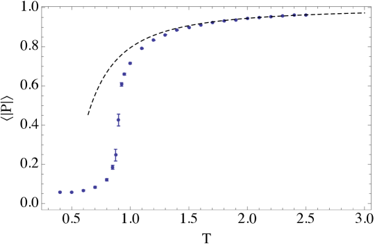
Figure 1: A Plot of the expectation value of the Polyakov loop $|P|$ as a function of the temperature, for $N=16$ and lattice spacing $a\approx 0.05$. One can see that near $T\approx 0.90$ the theory undergoes a second order phase transition.

In figure 2 we present plots of the energy and “extent of space” as functions of the temperature, for $N=16$ and lattice spacing $a\approx 0.05$. The dashed curves represent the analytical high temperature behaviour obtained in Kawahara:2007ib . Our results agree very well with the corresponding studies in Kawahara:2007fn ; Mandal:2011hb ; Azuma:2014cfa .

A more detailed analysis of the temperature range close to the transition revealed that there are in fact two transitions. To uncover more detail on the nature of the phase transition the authors of Kawahara:2007fn analysed the distribution of the holonomy matrix near the phase transition and uncovered behaviour consistent with the Gross-Witten model Gross:1980he and concluded that the holonomy undergoes a transition from a uniform distribution at $T_{c2}\simeq 0.8758(9)$ to a gapped distribution at $T_{c2}=0.905(2)$.

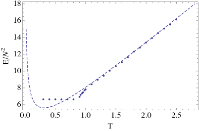
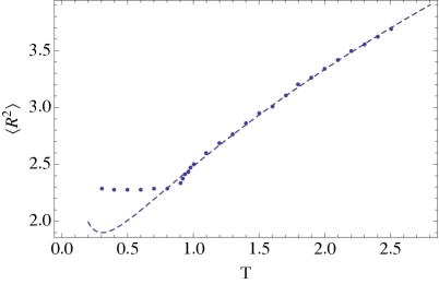
Figure 2: Plots of the scaled energy $E/N^{2}$ and the “extent of space” $\langle R^{2}\rangle$ as functions of the temperature. The dashed curves correspond to the high temperature behaviour obtained in Kawahara:2007ib . One can see that near $T\approx 0.9$ the plots suggest the existence of a second order phase transition. The energy and temperature in the plots are in units of $\lambda^{1/3}$.

In figure 3 we present our plots of the distribution of the holonomy around the phase transition. The dashed curves in the plot represent fits with the gapped and ungapped forms of the Gross-Witten distribution which are in excellent agreement with those of Kawahara:2007fn ; Mandal:2011hb ; Azuma:2014cfa . We have not attempted to refine their results, rather our purpose is to uncover a hidden Gaussian structure in the model.

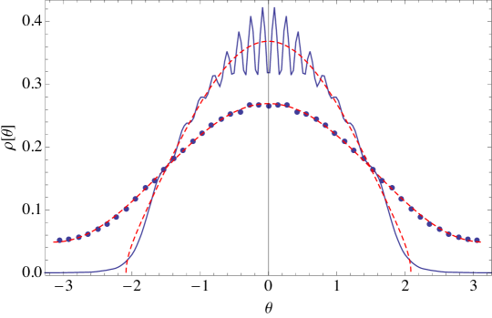
Figure 3: Plots of the distribution of the holonomy $P$ for temperatures $T=0.900$ (the confined or ungapped) and $T=.9006$ (the deconfinied or gapped). The plots are for size $N=16$ and lattice spacing $a\approx 0.05$. The dashed curves correspond to fits to the Gross-Witten gapped and ungapped distributions.

3.4 Gap and eigenvalue distribution

In this section we investigate the eigenvalue distribution of the scalar fields. We also perform studies of the mass of the theory at zero temperature. Our results suggest that at all temperatures the eigenvalue distribution of any one of the $X^{i}$ is given by a Wigner semicircle, with a radius $R_{\lambda}$ following the temperature behaviour of the observable $\langle R^{2}\rangle$. Therefore, we conclude that while the radius of the distribution experiences a phase transition the shape of the distribution remains unchanged. We believe that the main reason for this behaviour is that for nine scalar fields the commutator squared term can be replaced and approximated by a quadratic mass term in the spirit of Hotta:1998en , where an expansion at large number of scalar fields has been developed. Generalising these techniques, we are able to obtain an estimate of the mass, which agrees very well with both the gap measured from correlation functions and the radius of the distribution which are obtained from Monte Carlo simulations.

In the limit of high temperature the model reduces to the 10-dimensional Yang-Mills matrix model considered in Hotta:1998en . The obtained behaviour of the radius is in agreement with the large temperature expansion performed in Kawahara:2007ib and provides an analytic approximation to the leading coefficients in this expansion.

We begin by considering the model at zero temperature. In this case the holonomy can be completely gauged away and the model simplifies. Furthermore, at zero temperature the correlator:

$$\left\langle{\rm Tr}\left(X^{1}(0)X^{1}(t)\right)\right\rangle\propto e^{-m\,t}+\dots\ ,$$ (25)

captures the gap $\Delta m=E_{1}-E_{0}$ of the theory. To calculate the gap in the discrete theory, we periodically identify the time direction with period $\beta$:

$$\left\langle{\rm Tr}\left(X^{1}(0)X^{1}(t)\right)\right\rangle=A\,(e^{-m\,t}+e^{-m(\beta-t)})\ ,$$ (26)

Note that although formally $\beta$ is the same parameter that we have at finite temperature, since we set the holonomy to zero here its meaning is just a periodic coordinate as opposed to inverse temperature. Our result for the correlator for $N=30$, $\beta=10$ and lattice spacing $a=0.25$ is presented on the left in figure 4. The fitting curve is given by equation (26) and when we perform a two parameter fit we obtain $A\approx 7.50\pm 0.2$ and $m\approx(1.90\pm.01)\,\lambda^{1/3}\,$. However, for Gaussian scalar fields of mass $m$ we have $A=\frac{N}{2m(1-{\rm e}^{-\beta m})}$ and performing a one parameter fit for $m$ yields $m=1.965\pm 0.007$ and $A=7.63\pm 0.03$ On the right we have presented a plot of the eigenvalue distribution of one of the matrices for the same parameters. The fitting curve represents a Wigner semicircle of radius $R_{\lambda}\approx 1.01$. The fact that the theory is gapped and that the eigenvalue distribution is a semicircle suggests that that at low temperate the model has an effective action:

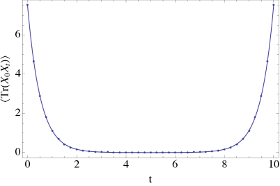
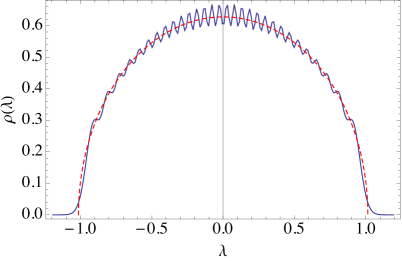
Figure 4: On the left: A plot of the correlator $\left\langle{\rm Tr}\left(X^{1}(0)X^{1}(t)\right)\right\rangle$ for $N=30$, $\beta=10$ and lattice spacing $a=0.25$. The fitting curve is given by equation (26) with $A=\frac{N}{2m(1-{\rm e}^{-\beta m})}$ and with parameters $m\approx(1.965\pm.007)\lambda^{1/3}\,$. On the right: A plot of the eigenvalue distribution of one of the scalars for the same parameters. The fitting curve represent a Wigner-semicircle of radius $R_{\lambda}\approx 1.01\,$.

$$S_{\rm eff}=N\int\limits_{-\infty}^{\infty}dt\,{\rm Tr}\left(\frac{1}{2}(\dot{X}^{i})^{2}+\frac{1}{2}m^{2}(X^{i})^{2}\right)$$ (27)

for each of the matrices $X^{i}$. It is well known Brezin:1977sv that for the action (27) the eigenvalue distribution of $X$ is given by a Wigner semicircle of radius:

$$R_{\lambda}=\sqrt{\frac{2}{m}}\approx 1.009\pm.002,$$ (28)

where we have substituted $m\approx 1.965\pm.007$. This agrees nicely (within errors) with the result for $R_{\lambda}\approx 1.01$ obtained by fitting the actual distribution. It is also in excellent agreement with the large $p$ theoretical prediction of Mandal:2011hb ,

$$R_{\lambda}(p)=\sqrt{\frac{2}{p^{1/3}}}(1+\frac{1}{p}(\frac{7\sqrt{5}}{30}-\frac{9}{32})+\cdots)\simeq 1.0068$$ (29)

3.5 $1/D$ expansion

Adapting the techniques developed in Hotta:1998en to the time dependent case that we are considering we can obtain a theoretical estimate of the radius at low temperature. Let us consider again the action of the bosonic model (5):

$$S_{b}=N\,\int_{0}^{\beta}dt\,{\rm tr}\left\{\frac{1}{2}({\cal D}_{t}{X^{i}})^{2}-\frac{1}{4}[X^{i},X^{j}]^{2}\right\}\ ,$$ (30)

where we have rescaled so that $\beta=\frac{\lambda^{1/3}}{T}$ (effectively we set $g=N^{-1/2}$). The commutator square term can be written as:

$${\rm Tr}[X^{i},X^{j}]^{2}={\rm Tr}\left([t^{a},t^{c}][t^{b},t^{d}]\right)X^{i}_{a}X^{i}_{b}\,X^{j}_{c}X^{j}_{d}=\lambda^{abcd}X^{i}_{a}X^{i}_{b}\,X^{j}_{c}X^{j}_{d}\ ,$$ (31)

where $t^{a}$ are $SU(N)$ generators normalised to ${\rm Tr\,}t^{a}t^{b}=\delta^{ab}$ and the tensor $\lambda^{abcd}$ is given by:

$$\lambda^{abcd}=\frac{1}{2}{\rm Tr}\left([t^{a},t^{c}][t^{b},t^{d}]+[t^{a},t^{d}][t^{b},t^{c}]\right)\ ,$$ (32)

It is convenient also to define the inverse kernel of $\lambda^{abcd}$ satisfying:

$$\mu_{abcd}\,\lambda^{cdef}=\delta_{a}^{e}\delta_{b}^{f}\ ,~{}~{}~{}\lambda^{abcd}\,\mu_{cdef}=\delta^{a}_{e}\delta^{b}_{f}\ .$$ (33)

We will also use the identities:

$$\lambda^{abcd}\,\delta_{cd}=-2N\,\delta^{ab}\ ,~{}~{}~{}~{}\mu_{abcd}\,\delta^{cd}=-\frac{1}{2N}\,\delta_{ab}\ .$$ (34)

The action (30) can then be written as:

$$S_{b}=N\,\int_{0}^{\beta}dt\,{\rm Tr}\left(\frac{1}{2}({\cal D}_{t}{X^{i}})^{2}\right)-\frac{N}{4}\lambda^{abcd}\int_{0}^{\beta}dt\,X^{i}_{a}X^{i}_{b}\,X^{j}_{c}X^{j}_{d}\ .$$ (35)

Our next step is to add to the action the term:

$$\Delta S=\frac{N}{4}\mu_{abcd}\int\limits_{0}^{\beta}dt\left(k^{ab}+\lambda^{abef}X^{i}_{e}X^{i}_{f}\right)\left(k^{cd}+\lambda^{cdgh}X^{i}_{g}X^{i}_{h}\right)\ ,$$ (36)

the action $S_{b}^{\prime}=S_{b}+\Delta S$ then becomes:

$$S_{b}^{\prime}=\frac{N}{2}\,\int_{0}^{\beta}dt\,\left\{{\rm Tr}({\cal D}_{t}{X^{i}})^{2}+k^{ab}X_{a}^{i}X_{b}^{i}\right\}+\frac{N}{4}\mu_{abcd}\int\limits_{0}^{\beta}\,dt\,k^{ab}k^{cd}\ .$$ (37)

Next we define:

$$k_{\,ij,lm}\equiv t_{ij}^{a}\,k^{ab}\,t_{lm}^{b}\ ,$$ (38)

From the definition of $k_{ij,lm}$ it follows that it is traceless with respect to the first and the second pair of indices and we can invert: $k^{ab}=t^{a}_{ij}\,k_{ji,ml}\,t^{b}_{lm}$. Substituting in the action (37), Fourier transforming (via $X=\sum_{n}e^{i\frac{2\pi n}{\beta}t}\tilde{X}_{n}$) and assuming $k_{ab}$ is time independent we obtain:

$$S_{b}^{\prime}=\frac{N}{2}\sum\limits_{n=-\infty}^{\infty}\tilde{X}_{-n,\,ij}\left(\left(\frac{2\pi\,n+\theta_{i}-\theta_{j}}{\beta}\right)^{2}P_{jl,ml}+k_{jl,ml}\right)\tilde{X}_{n,\,lm}+\frac{\beta\,N}{4}\mu_{abcd}\,k^{ab}k^{cd}\ ,$$ (39)

where we have defined the projector on traceless matrices:

$$P_{ij,lm}=t_{ij}^{a}\,t^{a}_{lm}=\delta_{im}\delta_{jl}-\frac{1}{N}\delta_{ij}\delta_{lm}\$$ (40)

and assumed that $k$ is constant. Defining also the double index matrix :

$$W(n)_{ij,lm}\equiv\left(\frac{2\pi\,n+\theta_{i}-\theta_{j}}{\beta}\right)^{2}P_{jl,ml}+k_{jl,ml}\ ,$$ (41)

we can integrate out the X’s:

$$\int{\cal D}X\,{\cal D}k\,e^{-S_{b}^{\prime}}\propto\int{\cal D}k\,\prod_{n}{\rm Det}^{-{p}/{2}}\left(P.W(n).P\right)e^{-\frac{\beta\,N}{4}\mu_{abcd}\,k^{ab}k^{cd}}\ .$$ (42)

The effective action for the field $k$ then becomes:

$$S_{\rm eff}[k]=\frac{p}{2}\sum\limits_{n}{\rm Tr}\log\left(P.W(n).P\right)+\frac{\beta\,N}{4}\mu_{abcd}\,k^{ab}k^{cd}\ .$$ (43)

We now notice that the first term in the expression for the matrix $W$ (41) commutes with the projector $P$. It is natural then to consider an ansatz for $k$ which also have that property. Thus we consider:

$$k_{ij,lm}\equiv k_{ij}\,P_{ij,lm}=P_{ij,lm}\,k_{lm}\,$$ (44)

The last equality is possible only if all diagonal components of $k_{ij}$ are the same (namely $k_{ii}=k_{jj}$ for all $i,j$) we also choose $k_{ij}$ to be symmetric. Then:

$$W(n)_{ij,lm}=\Delta_{ij}(n)\,P_{ij,lm}=\,P_{ij,lm}\Delta_{lm}(n)\ ,$$ (45)

$$\Delta_{ij}(n)\equiv\left(\frac{2\pi\,n+\theta_{i}-\theta_{j}}{\beta}\right)^{2}+k_{ij}\ ,$$

and we have for all powers $r$ that $(P.W(n).P)_{ij,lm}^{r}=P_{ij,lm}\,(\Delta_{ij}(n))^{r}$. Therefore,

$$S_{\rm eff}[k]=\frac{p}{2}\sum_{n}\sum_{ij}P_{ij,ji}\log(\Delta(n)_{ij})+\frac{\beta\,N}{4}\mu_{abcd}\,k^{ab}k^{cd}\ .$$ (46)

The corresponding saddle point equation $S_{\rm eff}^{\prime}[k]=0$ becomes:

$$\frac{p}{2}\sum_{n}\frac{P_{ij,ji}}{\left(\frac{2\pi\,n+\theta_{i}-\theta_{j}}{\beta}\right)^{2}+k_{ij}}+\frac{\beta\,N}{2}\mu_{abcd}\,k^{ab}t^{c}_{ij}t^{d}_{ji}=0\ .$$ (47)

We can now sum the series to obtain:

$$\frac{p}{\sqrt{k_{ij}}}\,\frac{\sinh(\beta\sqrt{k_{ij}})}{\cosh(\beta\sqrt{k_{ij}})-\cos(\theta_{i}-\theta_{j})}P_{ij,ji}+{2N}\mu_{abcd}\,k^{ab}t^{c}_{ij}t^{d}_{ji}=0\ .$$ (48)

In principle we can solve for $k_{ij}$ in terms of $\theta_{i}-\theta_{j}$, but we will restrict ourselves to extract the low temperature dependence. The first term in equation (48) has the following expansion:

$$\frac{\sinh(\beta\sqrt{k_{ij}})}{\cosh(\beta\sqrt{k_{ij}})-\cos(\theta_{i}-\theta_{j})}=1+2\cos(\theta_{i}-\theta_{j})\,e^{-\beta\sqrt{k_{ij}}}+O(e^{-2\,\beta\sqrt{k_{ij}}})$$ (49)

One can see that the effect of the holonomy is exponentially suppressed at low temperature, To leading order we can then consider a symmetric ansatz $k_{ij}=k_{0}$, which also implies $k^{ab}=k_{0}\,\delta^{ab}$. We obtain:

$$\frac{p}{\sqrt{k_{0}}}P_{ij,ji}-k_{0}\,P_{ij,ji}=0~{}~{}\therefore k_{0}=p^{2/3}\ .$$ (50)

Substituting into the action (37) to leading order we obtain:

$$S_{b}=N\int\limits_{-\infty}^{\infty}dt\,{\rm Tr}\left(\frac{1}{2}(\dot{X}^{i})^{2}+\frac{p^{2/3}}{2}(X^{i})^{2}\right)$$ (51)

and the corresponding radius of the eigenvalue distribution is:

$$R_{0}=\left(\frac{8}{p}\right)^{1/6}\approx 0.98\ .$$ (52)

This result agrees within a few percent with $R_{\lambda}\approx 1.01$ obtained by fitting the distribution in figure 4.

The exponential suppression of the holonomy corrections to the low temperature saddle point for $k^{ab}$ suggest that a lot of the physics of the model (at least at low temperature) can be captured by the action:

$$S_{b}=N\int\limits_{0}^{\beta}dt\,{\rm Tr}\left(\frac{1}{2}({\cal D}_{t}X^{i})^{2}+\frac{p^{2/3}}{2}(X^{i})^{2}\right)\ ,$$ (53)

where we restored the gauge field in the covariant derivatives. Surprisingly this model knows lots about the phase transition of the full model. An analysis similar to that above shows that the critical temperature for $p$ adjoint gauged Gaussian matrices as in Mandal:2009vz with mass $m$ occurs at $T_{c}^{Gaussian}=\frac{m}{\ln p}$ which for $m=p^{1/3}$ yields $Tc=0.9467$. In figure 5 we have presented our results for the energy and the Polyakov loop. Note that in this approximation the scaled energy $E/N^{2}$ is equal to the extent of space $\langle R^{2}\rangle$.

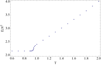
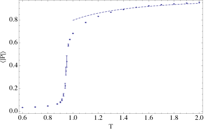
Figure 5: On the left: A plot of the energy of the gauged gaussian model for $N=32$ lattice spacing $a\approx 0.05$. The red curve represents Wigner semicircle. On the right: A plot of the expectation value of the Polyakov loop for $N=32$ lattice spacing $a\approx 0.05$. The second order phase transition takes place at $T\approx 0.95$. The energy and temperature in the plots are in units of $\lambda^{1/3}$.

The plots are for $N=32$ and lattice spacing $a\approx 0.05$. One can see that both the energy and the Polyakov loop exhibit the same behaviour as for the full model. There again appear to be two distinct transitions with the higher temperature one taking place at $T\approx.95$ and again appearing to be second order. It is slightly shifted towards high temperatures relative to the critical temperature for the full model. If instead of mass $m=p^{1/3}\lambda^{1/3}$ we use the value $m\simeq(1.90\pm.01)\lambda^{1/3}$ the phase transition is shifted in the opposite direction (just bellow $T=0.9$). This indicates that if one fits the mass parameter one can improve even further the agreement of the gauged gaussian model and the full one. The dashed curve in the second plot is the theoretical prediction for the high-temperature behaviour of the Polyakov loop, again one can observe a very good agreement. The high temperature behaviour of the energy on the other side disagrees with the corresponding behaviour of the full model. This is not surprising since we derived the effective action at low temperature and the dominant behaviour at high temperature is dominated by the highest power of the potential which has been changed from quartic to quadratic.

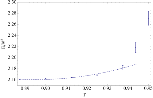
Figure 6: A zoomed in plot of the energy versus the temperature. The dashed curve represents a fit to equation (54) with $T_{0}\approx 0.896$.

One can also see that at low temperature the energy remains constant.

In figure 6 we have presented a plot of the energy versus the temperature zoomed in near the phase transition. The dashed curve represents a fit with:

$$E-\epsilon_{0}=C(T-T_{0})^{2}$$ (54)

with parameter $T_{0}\approx 0.896$. This indicates that the third order phase transition that the full model exhibits Kawahara:2007fn ; Mandal:2011hb is also captured by the gauged gaussian model.

One can perform the large $p$ analysis (see Hotta:1998en ) in the high temperature limit where the model now has $p+1$ matrices (the holonomy becomes the additional matrix) and predict that the model in this limit again becomes Gaussian but now the field $k_{ab}$ includes the holonomy and the saddle becomes $k_{ab}=\sqrt{p+1}\delta_{ab}$ which again predicts a Gaussian matrix model with a high temperature effective action $S_{eff}=\frac{\sqrt{p+1}}{2}Tr((X^{i})^{2})$ and consequently a Wigner semicircle distribution for the eigenvalues os $X^{i}$.

We conclude this section by presenting results for the eigenvalue distribution of the gauged gaussian model at finite temperature. In figure 7 we presented plots of the distribution for $T=0.2$, $N=30$ (left) and $T=5.0$, $N=30$ (right). The red dashed curves show a Wigner semicircle. One can see that the shape of the eigenvalue distribution does not change with temperature.

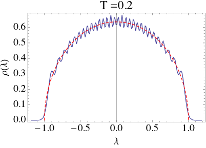
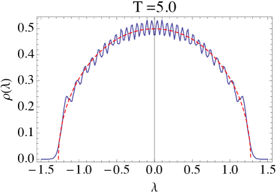
Figure 7: On the left: A plot of the eigenvalue distribution for $N=30$, $T=.2$ and lattice spacing $a=.25$. The red curve represents Wigner semicircle. On the right: A plot of the eigenvalue distribution for $N=30$, $T=5.0$ and lattice spacing $a=.05$. Again the red curve represents Wigner semicircle.

4 The supersymmetric model on the lattice

In this section we consider the full supersymmetric BFSS model on the lattice. The model has been simulated using non-lattice approach in Anagnostopoulos:2007fw and using lattice discretisation in Catterall:2008yz and Kadoh:2015mka . The main goal of these studies has been to compare the low temperature regime of the model to the holographically dual black hole geometry. The authors of refs. Anagnostopoulos:2007fw and Kadoh:2015mka also compared the high temperature regime of the model with the high temperature expansion performed in Kawahara:2007ib . Our goal is to reproduce some of these studies and calibrate our code.

A naive discretisation of the action (4) would result in a fermion doubling. This can be avoided  Catterall:2008yz if the charge conjugation matrix is taken to be $C_{9}=1_{8}\otimes\sigma_{1}$. Constructing a basis for which $C_{9}$ is of this form is relatively straightforward. For example one can tensor up the Majorana basis in seven euclidean dimensions $\tilde{\gamma}_{E}^{a}$:

$$\gamma^{a} = -\tilde{\gamma}_{E}^{a}\otimes\sigma_{3}\ ,~{}~{}~{}{\rm for}~{}a=1,\dots,7\ ,$$

$$\gamma^{8} = 1_{8}\otimes\sigma_{2}\ ,$$

$$\gamma^{9} = 1_{8}\otimes\sigma_{1}\ ,$$ (55)

and verify that indeed $C_{9}$ is of the desired form (it also satisfies $C_{9}=\gamma^{9}$). We next proceed in discretising the action (4). Since the bosonic part of the action is identical to the one considered in section 3 , we will consider only the fermionic part of the action:

$$S_{f}=\frac{1}{2g^{2}}\int d\tau\,{\rm tr}\left\{\psi^{\alpha}C_{9\,\alpha\beta}\,{\cal D}_{\tau}\psi^{\beta}-\psi^{\alpha}(C_{9}\gamma^{i})_{\alpha\beta}\,[X^{i},\psi^{\beta}]\right\}\ .$$ (56)

We begin by splitting the fermions into two eight component fermions: $\psi=(\psi_{1},\psi_{2})$ and defining the forward and backward derivatives $D_{\pm}$:

$$({\cal D}_{-}W)_{n} = (W_{n}-U_{n,n-1}W_{n-1}U_{n-1,n})/{a}\ ,$$

$$({\cal D}_{+}W)_{n} = (U_{n,n+1}W_{n+1}U_{n+1,n}-W_{n})/{a}\ .$$ (57)

One can show that the discretised kinetic term then becomes:

$$S_{f}^{\rm kin} = \frac{1}{2g^{2}}\int d\tau\,{\rm tr}\left(\psi^{\alpha}C_{9\,\alpha\beta}\,{\cal D}_{\tau}\psi^{\beta}\right)=\frac{a}{2g^{2}}\sum_{n=0}^{\Lambda-1}{\rm tr}\left\{\psi_{1,n}^{T}({\cal D}_{-}\psi_{2})_{n}+\psi_{2,n}^{T}({\cal D}_{+}\psi_{1})_{n}\right\}=$$

$$=\frac{1}{g^{2}}{\rm tr}\left\{-\sum_{n=0}^{\Lambda-1}\psi^{T}_{2,n}\psi_{1,n}+\sum_{n=0}^{\Lambda-2}\psi^{T}_{2,n}U_{n,n+1}\psi_{1,n+1}U_{n+1,n}\pm\psi^{T}_{2,\Lambda-1}U_{\Lambda-1,0}\psi_{1,0}U_{0,\Lambda-1}\right\}\,\,\ ,$$

where the plus/minus sign in the last term corresponds to periodic/anti-periodic boundary conditions for the fermions. Using the gauge from the previous subsection when the holonomy is concentrated on a singe link we can write $S_{f}^{\rm kin}$ as:

$$S_{f}^{\rm kin}=\frac{1}{g^{2}}{\rm tr}\left\{-\sum_{n=0}^{\Lambda-1}\psi^{T}_{2,n}\psi_{1,n}+\sum_{n=0}^{\Lambda-2}\psi^{T}_{2,n}\psi_{1,n+1}\pm\psi^{T}_{2,\Lambda-1}D\,\psi_{1,0}\,D^{\dagger}\right\}\ .$$ (59)

Since all fields transform in the adjoint of $SU(N)$ instead of dealing with matrices we can use the corresponding real components: $X^{a}={\rm tr}(t^{a}X)$ and $\psi^{a}={\rm tr}(t^{a}\psi)$, where $t^{a}$ are the standard basis of $SU(N)$ (introduced earlier) normalised as ${\rm tr}\,t^{a}t^{b}=\delta^{ab}$. $S_{f}^{\rm kin}$ can then be written as:

$$S_{f}^{\rm kin} = \frac{1}{g^{2}}\sum_{a,b=0}^{N^{2}-1}\sum_{m,n=0}^{\Lambda-1}\sum_{\alpha=1}^{8}\psi^{\alpha+8}_{m\,,a}K^{ab}_{mn}\psi^{\alpha}_{n\,,b}\ ,$$ (60)

$$K_{mn}^{ab} = (\delta_{m+1,n}-\delta_{m,n})\delta^{ab}\pm\delta_{m,\Lambda-1}\delta_{n,0}\,d^{ab}$$ (61)

$$d^{ab} = {\rm tr}\left(t^{a}\,D\,t^{b}\,D^{\dagger}\right)\ .$$ (62)

where the plus/minus sign corresponds to periodic/ant-periodic boundary conditions. The kinetic term can also be written as:

$$S_{f}^{\rm kin} = \sum_{a,b=0}^{N^{2}-1}\sum_{m,n=0}^{\Lambda-1}\sum_{\alpha,\beta=1}^{16}\psi^{\alpha}_{m\,,a}\,{\cal M}^{\rm kin}_{mn,\alpha\beta,ab}\,\psi^{\beta}_{n\,,b}$$ (63)

$${\cal M}^{\rm kin}_{mn,\alpha\beta,ab} = \frac{1}{2g^{2}}\left(\begin{array}[]{cc}0_{8}&-K_{nm}^{ba}\\ K_{mn}^{ab}&0_{8}\end{array}\right)_{\alpha\beta}\ .$$ (66)

Discretising the potential part of the action is straightforward. One obtains:

$$S_{f}^{\rm pot} = \sum_{a,b=0}^{N^{2}-1}\sum_{m,n=0}^{\Lambda-1}\sum_{\alpha,\beta=1}^{16}\psi^{\alpha}_{m\,,a}\,{\cal M}^{\rm pot}_{mn,\alpha\beta,ab}\,\psi^{\beta}_{n\,,b}$$ (67)

$${\cal M}^{\rm pot}_{mn,\alpha\beta,ab} = \frac{1}{2g^{2}}\,a\,if^{abc}\,(C_{9}\gamma^{i})_{\alpha\beta}\,X^{c,i}_{n}\delta_{n+m,0}\ .$$ (68)

Finally, defining:

$${\cal M}_{mn,\alpha\beta,ab} = \frac{1}{2g^{2}}\left(\begin{array}[]{cc}0_{8}&-K_{nm}^{ba}\\ K_{mn}^{ab}&0_{8}\end{array}\right)_{\alpha\beta}+\frac{1}{2g^{2}}\,a\,if^{abc}\,(C_{9}\gamma^{i})_{\alpha\beta}\,X^{c,i}_{n}\delta_{n+m,0}\ .$$ (71)

We can write:

$$S_{f}=\psi^{T}{\cal M}\psi\ .$$ (72)

4.1 The Pfaffian phase is not a problem!

Integrating out the Fermions, the partition function of the model can be written as:

$${\cal Z}\propto\int{\cal D}X\,{\cal D}\psi\,e^{-S[X,\psi]}\propto\int{\cal D}X\,{\rm Pf}({\cal M})\,e^{-S_{\rm bos}[X]}$$ (73)

Observe that ${\cal M}$ is the sum of an anti-hermitian kinetic term and a hermitian potential and ${\cal M}^{\dagger}(X)=-{\cal M}(-X)$. Also because the Bosonic action is symmetric in $X$ the Pfaffian in the partition function can be replaced by $|{\rm Pf}({\cal M})|\cos(\Theta_{Pf})$. Now as long as $-\frac{\pi}{2}<\Theta_{Pf}<\frac{\pi}{2}$ the cosine is positive and the effective action defines a true probability distribution given by

$$S_{eff}=S_{\rm bos}[X]-\ln|{\rm Pf}({\cal M})|-\ln\cos(\Theta_{Pf})$$ (74)

In figure 8 we presented plot of the phase of the pfaffian of the fermionic matrix for $N=3$ and four lattice points. One can see that the cosine remains positive. We believe that the drop in the $\cos\theta$ curve at very low temperatures is a lattice effect and is not present in the continuum limit. Our results show a very good agreement with the earlier studies of ref. Catterall:2009xn .

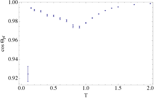
Figure 8: A plot of the phase of the pfaffian of the fermionic matrix for $N=3$ and $\Lambda=4$. One can see that the phase remains small for all temperature, but drops at ver low temperatures. We believe that this is a lattice artifact and is not present in the continuum limit. The flat directions are controlled with a small mass regulator at low temperature.

4.2 RHMC and fermionic forces

The next step is to apply the RHMC method Clark:2004cp to the model. To this end we need the so called fermionic forces. Let us summarise briefly the philosophy.

As we have shown above the model does not suffer from a severe sign problem and so we ignore the phase of the Pfaffian and use that:

$$|{\rm Pf}({\cal M})|={\rm det}({\cal M}^{\dagger}\,{\cal M})^{1/4}\ ,$$ (75)

to write

$${\cal Z}\propto\int{\cal D}X\,{\cal D}\xi^{\dagger}\,{\cal D}\xi\,e^{-S_{\rm bos}[X]-S_{\rm ps.f}}\ ,$$ (76)

where

$$S_{\rm ps.f}\equiv\xi^{\dagger}\,({\cal M}^{\dagger}\,{\cal M})^{-1/4}\xi\ .$$ (77)

Here $\xi$ is a $16(N_{c}^{2}-1)\Lambda$ dimensional vector consisting of the pseudo-fermionic fields. The idea of the RHMC is to approximate the rational exponent of the matrix ${\cal M}^{\dagger}\,{\cal M}$ with a partial sum:

$$({\cal M}^{\dagger}\,{\cal M})^{\delta}=\alpha_{0}+\sum_{i=1}^{\#}\alpha_{i}\,({\cal M}^{\dagger}\,{\cal M}+\beta_{i})^{-1}\ ,$$ (78)

where the parameters $\alpha_{0},\alpha_{i},\beta_{i}$ and $\#$ depend on the rational exponent $\delta$, the spectral range of the matrix ${\cal M}^{\dagger}\,{\cal M}$ and the desired accuracy. We will need two rational exponents. To update the pseudo fermions we use that the field $\eta\equiv({\cal M}^{\dagger}\,{\cal M})^{-1/8}\xi$ has a gaussian distribution and solve for $\xi=({\cal M}^{\dagger}\,{\cal M})^{1/8}\,\eta$ using a multi-shift solver. Therefore, $\delta=1/8$ is one of the rational exponents that we need. To calculate the fermionic forces and the contribution to the hamiltonian we need to invert $({\cal M}^{\dagger}\,{\cal M})^{-1/4}$ and the second exponent is $\delta=-1/4$.

Let us elaborate on the computation of the fermionic forces. We have two type of forces: gradients with respect to $X_{n\,ij}$ and gradients with respect to the phases of the links $\theta_{i}$. Using the partial expansion (78), one can easily derive expression for the derivatives of the fermionic action:

$$\frac{\partial S_{\rm ps.f}}{\partial u} = -\sum_{i=1}^{\#}\alpha_{i}\,\xi^{\dagger}({\cal M}^{\dagger}\,{\cal M}+\beta_{i})^{-1}\,\frac{\partial({\cal M}^{\dagger}\,{\cal M})}{\partial u}\,({\cal M}^{\dagger}\,{\cal M}+\beta_{i})^{-1}\xi$$ (79)

$$=-\sum_{i=1}^{\#}\alpha_{i}\,h_{i}^{\dagger}\,\frac{\partial({\cal M}^{\dagger}\,{\cal M})}{\partial u}\,h_{i}\ ,$$

where $h_{i}$ satisfy $({\cal M}^{\dagger}\,{\cal M}+\beta_{i})\,h_{i}=\xi_{i}$ and are obtained from the multi-solver.

4.3 Simulation results

In this subsection we provide our results from the Monte Carlo simulation of the model. We focus on the same observables that we analysed for the bosonic model in section 3.3. The definitions of the extent of space $\langle R^{2}\rangle$ and the expectation value of the Polyakov loop $P$ remain the same. The expression for the internal energy is Catterall:2008yz :

$$\frac{E}{N^{2}}=-\frac{3T}{N^{2}}\left(\langle S_{\rm bos}\rangle-\frac{9}{2}\Lambda\,(N^{2}-1)\right)\ ,$$ (80)

We have simulated the following configurations. For temperatures $T>2$ we have used $N=8$ and $\Lambda=8$. For the region $1\leq T\leq 2$ we have used $N=8$ and two or three different sizes of the lattice (for each point) in the range $8\leq\Lambda\leq 16$ (For $T=1$ we also went to $\Lambda=32$). For temperatures lower than one we have used $N=10,12,14$ and two lattice sizes per point $\Lambda=8,16$. For all temperatures the Polyakov loop is largely independent on the lattice spacing. The extent of space also experience very weak lattice effects. However, this is not the case for the internal energy and even for temperatures as high as $T=2$ lattice effects can be a factor. In figure 9 w present our results for the energy at $T=.9,1.0$ for different lattice spacing. One can see that the lattice effects die out linearly, which allows us to extrapolate the energy to zero lattice spacing. Our results for the internal energy are summarised in figure 10. The dashed curve at high temperatures is the theoretical curve obtained in the high temperature expansion. The dashed curve at low temperature represents the prediction of AdS/CFT. The model becomes unstable for small matrix sizes $N$, an effect which has been related to Hawking radiation in the dual gravitational theory Catterall:2009xn ; Hanada:2013rga . To compare with the AdS/CFT predictions one needs to consider large matrices. Simulations with large matrix sizes is computationally expensive and as a result our low temperature data is still preliminary. However, even at this point we have excellent overall agreement with the studies of Anagnostopoulos:2007fw and Kadoh:2015mka .

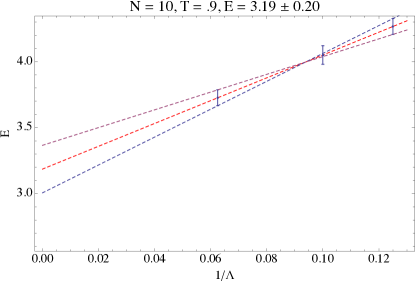
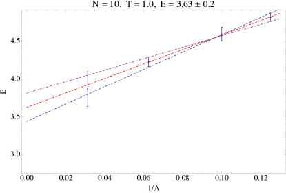
Figure 9: Scaling of the internal energy with the lattice spacing for temperatures $T=0.9,1.0$ and $N=10$. One can see that the lattice effects dies our linearly, which allows extrapolation of the zero lattice spacing result.

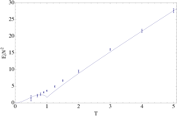
Figure 10: Results for the internal energy for $8\leq N\leq 14$ and $8\leq\Lambda\leq 16$. The dashed curve at high temperature correspond to the theoretical results of Kawahara:2007ib , while the low temperature curve represent the prediction for the internal energy from the AdS/CFT correspondence.

Finally, in figure 11 we present our results for the Polyakov loop and the extent of space. Again the dashed curve represents the high temperature theoretical result obtained in Kawahara:2007ib . One can see the excellent agreement at high temperatures. Our result for these observables agree with the previous studies preformed in Anagnostopoulos:2007fw , Catterall:2008yz , Hanada:2008ez and Kadoh:2015mka .

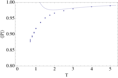
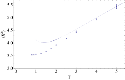
Figure 11: Plots of the expectation value of the Polyakov loop $\langle|P|\rangle$ and the extent of space $\langle R2\rangle$ as functions of temperature. The dashed curves represent the predictions of the high temperature expansion.

5 Discussion

In this paper we have analysed both the purely Bosonic and the supersymmetric BFSS models. These are “Hoppe” regulated membranes and one would expect that in the large $N$ limit when the regulator is removed that they describe the full quantum dynamics of these membranes. Surprisingly we found that the bosonic model, for sufficiently large embedding dimension reduces to a system of $p$-massive free bosons with the mass given by $m\sim p^{1/3}$. For $p=9$ we performed detailed simulations of the model evaluating both the fall off of the correlation function and the eigenvalue distribution of the $X^{i}$ fit with a Wigner semi-circle both of which give a consistent mass $m\simeq(1.965\pm.007)\lambda^{1/3}$. This is a fundamental non-perturbative result and gives the mass gap in the full Hamiltonian of the model.

The correspondence of the full and gauged Gaussian model is excellent for a wide range of temperatures. Somewhat surprisingly the phase transition region of the full model is faithfully reproduced by the effective model with the two transitions of the full model merged into one. Since the finite temperature version of the model is also the high temperature limit of $1+1$ dimensional maximally supersymmetric Yang-Mills Aharony:2004ig compactified on a circle, we have established that this latter model should also reduce to a system of free massive scalars in its large radius high temperature phase.

We then study the full supersymmetric BFSS model using a rational hybrid monte carlo simulation with Fourier acceleration to evaluate observables of the model. After describing our lattice discretisation of the model we investigated the phase of the Pfaffian obtained on integrating out the Fermions. The Pfaffian is generically complex, however, its phase is in fact not a problem for simulations. What enters simulations is the cosine of this phase and in the regularisation used in our work this phase is in fact restricted to a region where the cosine is positive once the lattice spacing is sufficiently small. Direct measurements confirm that the phase is indeed small.

Though our results for this part of the paper do not yet go beyond those of Anagnostopoulos:2007fw or cover as low a temperature as those of Kadoh:2015mka they are more precise than those of Catterall and Wiseman Catterall:2008yz who use a similar lattice simulation. We have taken several lattice spacings and then performed an extrapolation to the limit of zero lattice spacing. We find good agreement with earlier results and excellent agreement with the predictions of AdS/CFT once $1/\alpha^{\prime}$ corrections are included. Our results appear to approach the predictions of AdS/CFT a little more closely than those of Anagnostopoulos:2007fw but the difference is broadly within the errors. The principal difficulty in simulating the model at lower temperatures is due to critical slowing down and though Fourier acceleration helped for $T\simeq 0.5$, simulations becomes increasingly more difficult at lower temperatures. An additional difficulty is the instability due to flat directions, which require increasingly larger matrix sizes as the temperature is reduced.

One of the principal aims of this work was to check the claims of previous work and in particular those on the absence of a complex phase problem. We were also interested in calibrating our code as we extend it to include systems with $D4$-branes. The extension to such systems will allow us to perform more extensive tests of the AdS/CFT correspondence.

Acknowledgements: We wish to thank S. Catterall, M. Panero and M. Hanada for helpful comments.

References

- (1) P. K. Townsend, “The eleven-dimensional supermembrane revisited”, Phys. Lett. B350 (1995) 184 [hep-th/9501068].
- (2) T. Banks, W. Fischler, S. H. Shenker and L. Susskind, “M theory as a matrix model: A Conjecture,” Phys. Rev. D 55, 5112 (1997) [hep-th/9610043].
- (3) L. Susskind, hep-th/9704080.
- (4) D. E. Berenstein, J. M. Maldacena and H. S. Nastase, “Strings in flat space and pp waves from N=4 Super Yang Mills,” AIP Conf. Proc. 646 (2003) 3.
- (5) O. Aharony, O. Bergman and D. L. Jafferis, “Fractional M2-branes,” JHEP 0811 (2008) 043 [arXiv:0807.4924 [hep-th]].
- (6) J. Hoppe “Quantum Theory Of A Massless Relativistic Surface And A Two Dimensional Bound State Problem”, Ph.D. Thesis, Massachusetts Institute of Technology, (1982).
- (7) B. de Wit, J. Hoppe and H. Nicolai, “On the Quantum Mechanics of Supermembranes,” Nucl. Phys. B 305 (1988) 545.
- (8) G. Mandal and T. Morita, “Phases of a two dimensional large N gauge theory on a torus,” Phys. Rev. D 84 (2011) 085007 doi:10.1103/PhysRevD.84.085007 [arXiv:1103.1558 [hep-th]].
- (9) G. Mandal, M. Mahato and T. Morita, “Phases of one dimensional large N gauge theory in a 1/D expansion,” JHEP 1002, 034 (2010) doi:10.1007/JHEP02(2010)034 [arXiv:0910.4526 [hep-th]].
- (10) T. Azuma, T. Morita and S. Takeuchi, “Hagedorn Instability in Dimensionally Reduced Large-N Gauge Theories as Gregory-Laflamme and Rayleigh-Plateau Instabilities,” Phys. Rev. Lett. 113 (2014) 091603 doi:10.1103/PhysRevLett.113.091603 [arXiv:1403.7764 [hep-th]].
- (11) S. Catterall, A. Joseph and T. Wiseman, “Thermal phases of D1-branes on a circle from lattice super Yang-Mills,” JHEP 1012, 022 (2010) [arXiv:1008.4964 [hep-th]].
- (12) J. R. Hiller, S. S. Pinsky, N. Salwen and U. Trittmann, Phys. Lett. B 624, 105 (2005) doi:10.1016/j.physletb.2005.08.003 [hep-th/0506225].
- (13) M. Baake, M. Reinicke and V. Rittenberg, “Fierz Identities for Real Clifford Algebras and the Number of Supercharges,” J. Math. Phys. 26 (1985) 1070.
- (14) R. Flume, “On Quantum Mechanics With Extended Supersymmetry and Nonabelian Gauge Constraints,” Annals Phys. 164 (1985) 189.
- (15) M. Claudson and M. B. Halpern, “Supersymmetric Ground State Wave Functions,” Nucl. Phys. B 250 (1985) 689.
- (16) E. Witten, “Bound states of strings and p-branes,” Nucl. Phys. B 460 (1996) 335 [hep-th/9510135].
- (17) D. B. Kaplan and M. Unsal, “A Euclidean lattice construction of supersymmetric Yang-Mills theories with sixteen supercharges,” JHEP 0509 (2005) 042 doi:10.1088/1126-6708/2005/09/042 [hep-lat/0503039].
- (18) S. Catterall and T. Wiseman, “Black hole thermodynamics from simulations of lattice Yang-Mills theory,” Phys. Rev. D 78, 041502 (2008) [arXiv:0803.4273 [hep-th]].
- (19) K. N. Anagnostopoulos, M. Hanada, J. Nishimura and S. Takeuchi, “Monte Carlo studies of supersymmetric matrix quantum mechanics with sixteen supercharges at finite temperature,” Phys. Rev. Lett. 100, 021601 (2008) [arXiv:0707.4454 [hep-th]].
- (20) M. Hanada, Y. Hyakutake, J. Nishimura and S. Takeuchi, Phys. Rev. Lett. 102, 191602 (2009) [arXiv:0811.3102 [hep-th]].
- (21) D. Kadoh and S. Kamata, “Gauge/gravity duality and lattice simulations of one dimensional SYM with sixteen supercharges,” arXiv:1503.08499 [hep-lat].
- (22) N. Kawahara, J. Nishimura and S. Takeuchi, “Phase structure of matrix quantum mechanics at finite temperature,” JHEP 0710, 097 (2007) [arXiv:0706.3517 [hep-th]].
- (23) Polchinski, Joseph. ”Frontmatter”, String Theory. 1st ed. Vol. 2. Cambridge: Cambridge University Press, 1998. pp. i-viii. Cambridge Books Online.
- (24) O. Aharony, J. Marsano, S. Minwalla and T. Wiseman, “Black hole-black string phase transitions in thermal 1+1 dimensional supersymmetric Yang-Mills theory on a circle,” Class. Quant. Grav. 21 (2004) 5169 [hep-th/0406210].
- (25) O. Aharony, J. Marsano, S. Minwalla, K. Papadodimas, M. Van Raamsdonk and T. Wiseman, JHEP 0601, 140 (2006) doi:10.1088/1126-6708/2006/01/140 [hep-th/0508077].
- (26) N. Kawahara, J. Nishimura and S. Takeuchi, “High temperature expansion in supersymmetric matrix quantum mechanics,” JHEP 0712, 103 (2007) [arXiv:0710.2188 [hep-th]].
- (27) D. J. Gross and E. Witten, “Possible Third Order Phase Transition in the Large N Lattice Gauge Theory,” Phys. Rev. D 21, 446 (1980). S. R. Wadia, “ = Infinity Phase Transition in a Class of Exactly Soluble Model Lattice Gauge Theories,” Phys. Lett. B 93, 403 (1980).
- (28) T. Hotta, J. Nishimura and A. Tsuchiya, “Dynamical aspects of large N reduced models,” Nucl. Phys. B 545, 543 (1999) [hep-th/9811220].
- (29) E. Brezin, C. Itzykson, G. Parisi and J. B. Zuber, “Planar Diagrams,” Commun. Math. Phys. 59, 35 (1978).
- (30) S. Catterall and T. Wiseman, JHEP 1004 (2010) 077 [arXiv:0909.4947 [hep-th]].
- (31) M. A. Clark, A. D. Kennedy and Z. Sroczynski, “Exact 2+1 flavour RHMC simulations,” Nucl. Phys. Proc. Suppl. 140, 835 (2005) [hep-lat/0409133].
- (32) M. Hanada, Y. Hyakutake, G. Ishiki and J. Nishimura, Science 344 (2014) 882 [arXiv:1311.5607 [hep-th]].