Marginal evidence for cosmic acceleration from Type Ia supernovae

Abstract

The ‘standard’ model of cosmology is founded on the basis that the expansion rate of the universe is accelerating at present — as was inferred originally from the Hubble diagram of Type Ia supernovae. There exists now a much bigger database of supernovae so we can perform rigorous statistical tests to check whether these ‘standardisable candles’ indeed indicate cosmic acceleration. Taking account of the empirical procedure by which corrections are made to their absolute magnitudes to allow for the varying shape of the light curve and extinction by dust, we find, rather surprisingly, that the data are still quite consistent with a constant rate of expansion.

I Introduction

In the late 1990’s, studies of Type Ia supernovae (SN Ia) showed that the expansion rate of the universe appears to be accelerating as if dominated by a cosmological constant ^{1; 2; 3}. Since then supernova cosmology has developed rapidly as an important probe of ‘dark energy’. Empirical corrections are made to reduce the scatter in the observed magnitudes by exploiting the observed (anti)correlation between the peak luminosity and the light curve width ^{4; 5}. Other such correlations have since been found e.g. with the host galaxy mass ⁶ and metallicity ⁷. Cosmological parameters are then fitted, along with the parameters determining the light curves, by simple $\chi^{2}$ minimisation ^{1; 8; 9; 10; 11}. This method has a number of pitfalls as has been emphasised earlier ^{12; 13}.

With ever increasing precision and size of SN Ia datasets, it is important to also improve the statistical analysis of the data. To accomodate model comparison, previous work ^{14; 15; 16} has introduced likelihood maximisation. In this work we present an improved maximum likelihood analysis, finding rather different results.

II Supernova cosmology

There are several approaches to making SN Ia ‘standardiseable candles’. The different philosophies lead to mildly different results but the overall picture seems consistent ¹⁷. In this paper we adopt the transparent approach of ‘Spectral Adaptive Lightcurve Template 2’ (SALT2) ^{18; 19} wherein the SN Ia are standardised by fitting their light curve to an empirical template, and the parameters of this fit are used in the cosmological analysis. Every SN Ia is assigned three parameters, one being $m^{*}_{B}$, the apparent magnitude at maximum (in the rest frame ‘$B$-band’), while the other two describe the light curve shape and colour corrections: $x_{1}$ and $c$. The distance modulus is then taken to be:

$$\mu_{\textrm{SN}}=m^{*}_{B}-M+\alpha x_{1}-\beta c,$$ (1)

where $M$ is the absolute magnitude, and $\alpha$ and $\beta$ are assumed to be constants for all SN Ia. These global constants are fitted along with the cosmological parameters. The physical mechanism(s) which give rise to the correlations that underlie these corrections remain uncertain ^{20; 21}. The SN Ia distance modulus is then compared to the expectation in the standard $\Lambda$CDM cosmological model:

$$\mu\equiv 25+5\log_{10}(d_{\textrm{L}}/\textrm{Mpc}),\quad\textrm{where:}$$

$$d_{\textrm{L}}=(1+z)\frac{d_{\textrm{H}}}{\sqrt{\Omega_{k}}}\textrm{sinh}\left(\sqrt{\Omega_{k}}\int_{0}^{z}\frac{H_{0}\textrm{d}z^{\prime}}{H(z^{\prime})}\right),$$

$$d_{\textrm{H}}=c/H_{0},\quad H_{0}\equiv 100h~{}\textrm{km}\,\textrm{s}^{-1}\textrm{Mpc}^{-1},$$

$$H=H_{0}\sqrt{\Omega_{\textrm{m}}(1+z)^{3}+\Omega_{k}(1+z)^{2}+\Omega_{\Lambda}},$$ (2)

where $d_{\textrm{L}},d_{\textrm{H}},H$ are the luminosity distance, Hubble distance and Hubble parameter respectively, and $\Omega_{\textrm{m}},\Omega_{\Lambda},\Omega_{k}$ are the matter, cosmological constant and curvature density in units of the critical density ³. There is a degeneracy between $H_{0}$ and $M_{0}$ so we fix the value of the Hubble parameter today to $h=0.7$ which is consistent with independent measurements.

III Maximum Likelihood Estimators

To find the maximum likelihood estimator (MLE) from the data, we must define the appropriate likelihood:

$$\mathcal{L}=\textrm{probability density}(\textrm{data}|\textrm{model}),$$

i.e. we have to first specify our model of the data. For a given SN Ia, the true data $(m^{*}_{B},x_{1},c)$ are drawn from some global distribution. These values are contaminated by various sources of noise, yielding the observed values $(\hat{m}^{*}_{B},\hat{x}_{1},\hat{c})$. Assuming the SALT2 model is correct, only the true values obey equation (1). However when the experimental uncertainty is of the same order as the intrinsic variance as in the present case, the observed value is not a good estimate of the true value. Parameterising the cosmological model by $\theta$, the likelihood function can be written as:

$${\mathcal{L}} =p[(\hat{m}^{*}_{B},\hat{x}_{1},\hat{c})|\theta]$$

$$=\int p[(\hat{m}^{*}_{B},\hat{x}_{1},\hat{c})|(M,x_{1},c),\theta]\ p[(M,x_{1},c)|\theta]\textrm{d}M\textrm{d}x_{1}\textrm{d}c,$$

which shows explicitly where the experimental uncertainties enter (first factor) and where the variances of the intrinsic distributions enter (second factor).

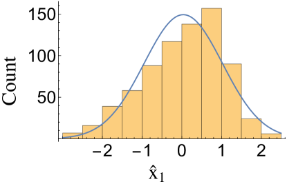
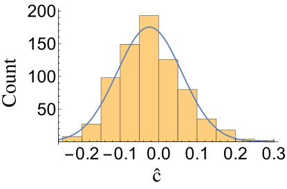
Figure 1: Distribution of the stretch and colour correction parameters in the JLA sample ¹¹, with gaussians superimposed.

Having a theoretically well-motivated distribution for the light curve parameters would be helpful, however this is not available. For simplicity we adopt global, independent gaussian distributions for all parameters, $M,x_{1}$ and $c$ (see Fig. 1), i.e. model their probability density as:

$$p[(M,x_{1},c)|\theta]=p(M|\theta)p(x_{1}|\theta)p(c|\theta),\quad\textrm{where:}$$

$$p(M|\theta)=(2\pi\sigma_{M_{0}}^{2})^{-1/2}\exp\left\{-\left[\left({M-M_{0}}\right)/\sigma_{M_{0}}\right]^{2}/2\right\},$$

$$p(x_{1}|\theta)=(2\pi\sigma_{x_{1,0}}^{2})^{-1/2}\exp\left\{-\left[\left({x_{1}-x_{1,0}}\right)/\sigma_{x_{1,0}}\right]^{2}/2\right\},$$

$$p(c|\theta)=(2\pi\sigma_{c_{0}}^{2})^{-1/2}\exp\left\{-\left[\left({c-c_{0}}\right)/\sigma_{c_{0}}\right]^{2}/2\right\}.$$ (4)

All 6 free parameters $\{M_{0},\sigma_{M_{0}},x_{1,0},\sigma_{x_{1,0}},c_{0},\sigma_{c_{0}}\}$ are fitted along with the cosmological parameters and we include them in $\theta$. Introducing the vectors $Y=\{M_{1},x_{11},c_{1},\dots M_{N},x_{1N},c_{N}\}$, the zero-points $Y_{0}$, and the matrix $\Sigma_{l}=\textrm{diag}(\sigma_{M_{0}}^{2},\sigma_{x_{1,0}}^{2},\sigma_{c_{0}}^{2},\dots)$, the probability density of the true parameters writes:

$$p(Y|\theta)={|2\pi\Sigma_{l}|}^{-1/2}\exp\left[-(Y-Y_{0})\Sigma_{l}^{-1}(Y-Y_{0})^{\textrm{T}}/2\right],$$ (5)

where $|\ldots|$ denotes the determinant of a matrix. What remains is to specify the model of uncertainties on the data. Introducing another set of vectors $X=\{m^{*}_{B1},x_{11},c_{1},\dots\}$, the observed $\hat{X}$, and the estimated experimental covariance matrix $\Sigma_{\textrm{d}}$ (including both statistical and systematic errors), the probability density of the data given some set of true parameters is:

$$p(\hat{X}|X,\theta)={|2\pi\Sigma_{\textrm{d}}|}^{-1/2}\exp\left[-(\hat{X}-X)\Sigma_{\textrm{d}}^{-1}(\hat{X}-X)^{\textrm{T}}/2\right].$$ (6)

To combine the exponentials we introduce the vector $\hat{Z}=\{\hat{m}^{*}_{B1}-\mu_{1},\hat{x}_{11},\hat{c}_{1},\dots\}$ and the block diagonal matrix

$$A=\begin{pmatrix}1&&0&0&\\ -\alpha&&1&0&0\\ \beta&&0&1&\\ &&0&\phantom{-1}&\ddots\end{pmatrix}.$$ (7)

With these, we have $\hat{X}-X=(\hat{Z}A^{-1}-Y)A$ and so $p(\hat{X}|X,\theta)=p(\hat{Z}|Y,\theta)$. The likelihood is then

$$\mathcal{L} =\int p(\hat{Z}|Y,\theta)\ p(Y|\theta)\textrm{d}Y$$

$$={|2\pi\Sigma_{\textrm{d}}|}^{-1/2}{|2\pi\Sigma_{l}|}^{-1/2}\int\textrm{d}Y$$

$$\times\exp\left(-(Y-Y_{0})\Sigma_{l}^{-1}(Y-Y_{0})^{\textrm{T}}/2\right)$$

$$\times\exp\left(-(Y-\hat{Z}A^{-1})A\Sigma_{d}^{-1}A^{\textrm{T}}(Y-\hat{Z}A^{-1})^{\textrm{T}}/2\right),$$

which can be integrated analytically to obtain:

$${\mathcal{L}} ={|2\pi(\Sigma_{\textrm{d}}+A^{\textrm{T}}\Sigma_{l}A)|}^{-1/2}$$

$$\times\exp\left[-(\hat{Z}-Y_{0}A)(\Sigma_{\textrm{d}}+A^{\textrm{T}}\Sigma_{l}A)^{-1}(\hat{Z}-Y_{0}A)^{\textrm{T}}/2\right].$$

This is the likelihood (equation (III)) for the simple model of equation (4), and the quantity which we maximise in order to derive confidence limits. The 10 parameters we fit are $\{\Omega_{\textrm{m}},\Omega_{\Lambda},\alpha,x_{1,0},\sigma_{x_{1,0}},\beta,c_{0},\sigma_{c_{0}},M_{0},\sigma_{M_{0}}\}$. We stress that it is necessary to consider all of these together and $\Omega_{\textrm{m}}$ and $\Omega_{\Lambda}$ have no special status in this regard. The advantage of our method is that we get a goodness-of-fit statistic in the likelihood which can be used to compare models or judge whether a particular model is a good fit. Note that the model is not just the cosmology, but includes modelling the distributions of $x_{1}$ and $c$.

With this MLE, we can construct a confidence region in the 10-dimensional parameter space by defining its boundary as one of constant $\mathcal{L}$. So long as we do not cross a boundary in parameter space, this volume will asymptotically have the coverage probability

$$p_{\textrm{cov}}=\int_{0}^{-2\log{\mathcal{L}}/{\mathcal{L}}_{\textrm{max}}}f_{\chi^{2}}(x;\nu)\textrm{d}x,$$ (10)

where $f_{\chi^{2}}(x;\nu)$ is the pdf of a chi-squared random variable with $\nu$ degrees of freedom, and $\mathcal{L}_{\textrm{max}}$ is the maximum likelihood. With 10 parameters in the present model, the values $p_{\textrm{cov}}\simeq\{0.68\;(``1\sigma"),0.95\;(``2\sigma")\}$ give $-2\log{\mathcal{L}}/{\mathcal{L}}_{\textrm{max}}\simeq\{11.54,18.61\}$ respectively.

To eliminate the so-called ‘nuisance parameters’, we set similar bounds on the profile likelihood. Writing the interesting parameters as $\theta$ and nuisance parameters as $\phi$, the profile likelihood is defined as

$$\mathcal{L}_{\textrm{p}}(\theta)=\max_{\phi}\mathcal{L}(\theta,\phi).$$ (11)

We substitute $\mathcal{L}$ by $\mathcal{L}_{\textrm{p}}$ in equation (10) in order to construct confidence regions in this lower dimensional space; $\nu$ is now the dimension of the remaining parameter space. Looking at the $\Omega_{\textrm{m}}-\Omega_{\Lambda}$ plane, we have for $p_{\textrm{cov}}\simeq\{0.68\;(``1\sigma"),0.95\;(``2\sigma"),0.997\;(``3\sigma")\}$, the values $-2\log\mathcal{L}_{\textrm{p}}/\mathcal{L}_{\textrm{max}}\simeq\{2.30,6.18,11.8\}$ respectively.

III.1 Comparison to other methods

It is illuminating to relate our work to previously used methods in SN Ia analyses. One method ¹⁴ maximises a likelihood, which is written in the case of uncorrelated magnitudes as

$$\tilde{\mathcal{L}}\propto\prod(2\pi\sigma_{\textrm{tot}}^{2})^{-1/2}\exp\left(-\Delta\mu^{2}/2\sigma_{\textrm{tot}}^{2}\right),$$ (12)

so it integrates over $\mu_{\textrm{SN}}$ to unity and can be used for model comparison. From Equation (III) we see that this corresponds to assuming flat distributions for $x_{1}$ and $c$. However the actual distributions of $\hat{x}_{1}$ and $\hat{c}$ are close to gaussian, as seen in Fig. 1. Moreover although this likelihood apparently integrates to unity, it accounts for only the $m_{B}^{*}$ data. Integration over the $x_{1},c$ data demands compact support for the flat distributions so the normalisation of the likelihood becomes arbitrary, making model comparison tricky.

More commonly used ^{1; 8} is the ‘constrained $\chi^{2}$’

$$\chi^{2}=\sum\Delta\mu^{2}/{(\sigma_{\mu}^{2}+\sigma_{\textrm{int}}^{2})},$$ (13)

but this cannot be used to compare models, since it is tuned to be 1 per degree of freedom for the $\Lambda$CDM model by adjusting an arbitrary error $\sigma_{\textrm{int}}$ added to each data point. This has been criticised ^{12; 13}, nevertheless the method continues to be widely used and the results presented without emphasising that it is intended only for parameter estimation for the assumed ($\Lambda$CDM) model, rather than determining if this is indeed the best model.

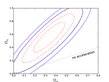
Figure 2: Contour plot of the profile likelihood in the $\Omega_{\textrm{m}}-\Omega_{\Lambda}$ plane. We show 1, 2 and 3$\sigma$ contours, regarding all other parameters as nuisance parameters, as red dashed lines, while the blue lines are 1 and 2$\sigma$ contours from the 10-dimensional parameter space projected on to this plane.

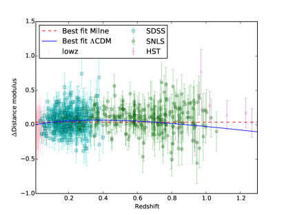
Figure 3: Comparison of the measured distance modulus with its expected value for the best fit accelerating universe ($\Lambda$CDM) and a universe expanding at constant velocity (Milne). The error bars include both experimental uncertainties and intrinsic dispersion. The bottom panel shows the residuals relative to the Milne model.

IV Analysis of JLA catalogue

Table 1: Maximum likelihood parameters under specific constraints (in boldface).

($-2\log\mathcal{L}_{\textrm{max}}=-214.97$) Constraint $-2\log\mathcal{L}/\mathcal{L}_{\textrm{max}}$ $\Omega_{\textrm{m}}$ $\Omega_{\Lambda}$ $\alpha$ $x_{1,0}$ $\sigma_{x_{1,0}}$ $\beta$ $c_{0}$ $\sigma_{c_{0}}$ $M_{0}$ $\sigma_{M_{0}}$ None (best fit) $\mathbf{0}$ 0.341 0.569 0.134 0.038 0.932 3.059 -0.016 0.071 -19.052 0.108 Flat geometry 0.147 0.376 $\mathbf{0.624}$ 0.135 0.039 0.932 3.060 -0.016 0.071 -19.055 0.108 Empty universe 11.9 $\mathbf{0.000}$ $\mathbf{0.000}$ 0.133 0.034 0.932 3.051 -0.015 0.071 -19.014 0.109 Non-accelerating 11.0 0.068 $\mathbf{0.034}$ 0.132 0.033 0.931 3.045 -0.013 0.071 -19.006 0.109 Matter-less universe 10.4 $\mathbf{0.000}$ 0.094 0.134 0.036 0.932 3.059 -0.017 0.071 -19.032 0.109 Einstein-deSitter 221.97 $\mathbf{1.000}$ $\mathbf{0.000}$ 0.123 0.014 0.927 3.039 0.009 0.072 -18.839 0.125

We focus on the Joint Lightcurve Analysis (JLA) catalogue ¹¹. (All data used are available on http://supernovae.in2p3.fr/sdss_snls_jla/ReadMe.html — we use the covmat_v6.) As shown already in Fig. 1, the distributions of the light curve fit parameters $\hat{x}_{1}$ and $\hat{c}$ are well modelled as gaussians. Maximisation of the likelihood under specific constraints is summarised in Table 1 and the profile likelihood contours in the $\Omega_{\textrm{m}}-\Omega_{\Lambda}$ plane are shown in Fig. 2. In Fig. 3 we compare the measured distance modulus, $\hat{\mu_{\textrm{SN}}}=\hat{m}^{*}_{B}-M_{0}+\alpha\hat{x}_{1}-\beta\hat{c}$ with its expected value in two cosmological models: ‘$\Lambda$CDM’ is the best fit accelerating universe while ‘Milne’ is an universe expanding with constant velocity. The error bars are the square root of the diagonal elements of $\Sigma_{l}+A^{\textrm{T}-1}\Sigma_{\textrm{d}}A^{-1}$ so include both experimental uncertainties and intrinsic dispersion. We show also the residuals with respect to the Milne model (which has been raised to take into account the change in $M_{0}$).

To assess how well our model describes the data, we present in Fig. 4 the ‘pull’ distribution. These are defined as the normalised, decorrelated residuals of the data,

$$\text{pulls}=(\hat{Z}-Y_{0}A)U^{-1},$$ (14)

where $U$ is the upper triangular Cholesky factor of the covariance matrix $\Sigma_{\textrm{d}}+A^{\textrm{T}}\Sigma_{l}A$. Performing a K-S test, comparing the pull distribution to a unit variance gaussian gives a p-value of $0.1389$.

To check the validity of our method and approximations, we do a Monte Carlo simulation of experimental outcomes from a model with parameters matching our best fit (see Table 1). Figure 5 shows the distribution of $-2\log[\mathcal{L}_{\textrm{true}}/\mathcal{L}_{\textrm{max}}]$, which is just as is expected.

V Discussion

That the SN Ia Hubble diagram appears consistent with an uniform rate of expansion has been noted earlier ^{22; 23; 24; 16}. We have confirmed this by a rigorous statistical analysis, using the JLA catalogue of 740 SN Ia processed by the SALT2 method. We find marginal (i.e. $\lesssim 3\sigma$) evidence for the widely accepted claim that the expansion of the universe is presently accelerating ³.

The Bayesian equivalent of this method (a “Bayesian Hierarchical Model”) has been presented elsewhere ¹³. We note that a Bayesian consistency test ²⁵ has been applied (albeit using the flawed ‘likelihood’ (equation 12) and ‘constrained $\chi^{2}$’ (equation 13) methods) to determine the consistency between the SN Ia data sets acquired with different telescopes ²⁶. These authors do find inconsistencies in the UNION2 catalogue but none in JLA. This test had been applied earlier to the UNION2.1 compilation finding no contamination, but those authors ²⁷ fixed the light curve fit ‘nuisance’ parameters, so their result is inconclusive. Including a ‘mass step’ correction for the host galaxies of SN Ia ¹¹ has little effect.

While our gaussian model (4) is not perfect, it appears to be an adequate first step towards understanding SN Ia standardisation. One might be concerned that various selection effects (e.g. Malmquist bias) affect the data. However to address this adequately is beyond the scope of this work. We are concerned here solely with performing the statistical analysis in an unbiased manner in order to highlight the different conclusion from previous analyses ¹¹ of the same data.

We wish to emphasise that whether the expansion rate is accelerating or not is a kinematic test and it is simply for ease of comparison with previous results that we choose to show the impact of doing the correct statistical analysis in the usual $\Lambda$CDM framework. In particular the ‘Milne model’ should not be taken literally to mean an empty universe since the deceleration due to gravity can in principle be countered e.g. by bulk viscosity associated with the formation of structure, resulting in expansion at approximately constant velocity even in an universe containing matter but no dark energy ²⁸. Such a cosmology is not prima facie in conflict with observations of the angular scale of fluctuations in the cosmic microwave background or of baryonic acoustic oscillations, although this does require further investigation. In any case, both of these are geometric rather than dynamical measures and do not provide compelling direct evidence for a cosmological constant — rather its value is inferred from the assumed ‘cosmic sum rule’: $\Omega_{\Lambda}=1-\Omega_{\textrm{m}}+\Omega_{k}$. This would be altered if additional terms due to the back reaction of inhomogeneities are included in the Friedmann equations ²⁹.

The CODEX experiment on the European Extremely Large Telescope aims to measure the ‘redshift drift’ over a 10-15 year period to determine whether the expansion rate is really accelerating ³⁰.

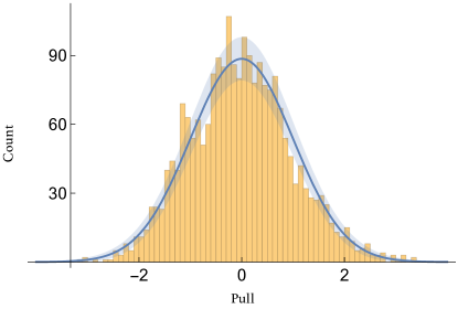
Figure 4: Distribution of pulls (14) for the best-fit model, compared to a normal distribution.

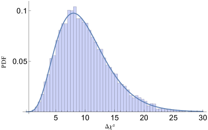
Figure 5: The distribution of the likelihood ratio from Monte Carlo, with a $\chi^{2}$ distribution with 10 d.o.f. superimposed.

Figure legends

Fig.1: Distribution of the stretch and colour correction parameters in the JLA sample ¹¹, with gaussians superimposed.

Fig.2: Contour plot of the profile likelihood in the $\Omega_{\textrm{m}}-\Omega_{\Lambda}$ plane. We show 1, 2 and 3$\sigma$ contours, regarding all other parameters as nuisance parameters, as red dashed lines, while the blue lines are 1 and 2$\sigma$ contours from the 10-dimensional parameter space projected on to this plane.

Fig.3: Comparison of the measured distance modulus with its expected value for the best fit accelerating universe ($\Lambda$CDM) and a universe expanding at constant velocity (Milne). The error bars include both experimental uncertainties and intrinsic dispersion. The bottom panel shows the residuals relative to the Milne model.

Fig.4: Distribution of pulls (14) for the best-fit model compared to a normal distribution.

Fig.5: The distribution of the likelihood ratio from Monte Carlo, with a $\chi^{2}$ distribution with 10 d.o.f. superimposed.

Methods: Confidence ellipsoids

The confidence ellipsoid is the collection of points $x=\{\Omega_{\text{m}},\Omega_{\Lambda},\alpha,x_{0},\sigma_{x_{0}}^{2},\beta,c_{0},\sigma_{c_{0}}^{2},M_{0},\sigma_{M_{0}}^{2}\}$, which obey

$$[x-x_{\text{MLE}}]\mathcal{F}[x-x_{\text{MLE}}]^{\text{T}}\leq\Delta\chi^{2},$$ (15)

where $\mathcal{F}$ is a symmetric matrix and $x_{\text{MLE}}$ is the MLE. The enclosed volume is a confidence region with coverage probability corresponding with high precision to the value obtained from Equation (10). The eigenvectors of $\mathcal{F}$ are then the principal axes of the ellipsoid, and the eigenvalues are the inverse squares of the lengths of the principal axes. We approximate this matrix with the sample covariance from the MC of section IV as $\mathcal{F}=\text{cov}(x,x)^{-1}$.

To make reading the matrix of eigenvectors easier, we round all numbers to 0.1. Thus, we get the following approximate eigenvectors of $\mathcal{F}$, in columns

$$\begin{array}[]{l}\Omega_{\text{m}}\\ \Omega_{\Lambda}\\ \alpha\\ x_{0}\\ \sigma_{x_{0}}^{2}\\ \beta\\ c_{0}\\ \sigma_{c_{0}}^{2}\\ M_{0}\\ \sigma_{M_{0}}^{2}\\ \end{array}\begin{pmatrix}0.5&0&0&0.8&0.1&-0.2&0&0&0&0\\ 0.8&0&0&-0.5&-0.1&0.2&0&0&0&0\\ 0&0&0&0&0&0&1&0&0&0\\ 0&0&0&-0.1&1&0&0&0&0&0\\ 0&0&1&0&0&0&0&0&0&0\\ 0&1&0&0&0&0&0&0&0&0\\ 0&0&0&0&0&0.1&0&1&0&0\\ 0&0&0&0&0&0&0&0&0&1\\ -0.1&0&0&0.3&0.1&1&0&0.1&0&0\\ 0&0&0&0&0&0&0&0&1&0\\ \end{pmatrix}$$ (16)

with respective lengths of semi-axes

$$10^{-3}\{172, 85.1,49.8,43.9,38.1,$$

$$9.89, 5.93,4.24,1.01,0.304\}$$ (17)

We also list the rounded correlation matrix,

$$\begin{pmatrix}\Omega_{\text{m}}\\ 0.9&\Omega_{\Lambda}\\ 0&0&\alpha\\ 0&0&0&x_{0}\\ 0&0&-0.1&0&\sigma_{x_{0}}^{2}\\ 0&0&0&0&0&\beta\\ 0.1&-0.1&0&0&0&0&c_{0}\\ 0&0&0&0&0&-0.3&0&\sigma_{c_{0}}^{2}\\ -0.2&-0.6&0&0&0&0.1&0.2&0&M_{0}\\ 0&0&-0.1&0&0&-0.3&0&0&0&\sigma_{M_{0}}^{2}\\ \end{pmatrix}$$ (18)

We see that the only pronounced correlations are between $\Omega_{\text{m}},\Omega_{\Lambda}$ and $M_{0}$. This is also apparent from Table 1.

Code availability

The code and data used in the analysis are available at: http://dx.doi.org/10.5281/zenodo.34487

Contributions

All authors participated in the analysis and in writing the paper.

Competing financial interests

The authors have no competing financial interests.

Corresponding author

Correspondence to: S. Sarkar

References

- (1) Perlmutter, S. et al. Measurements of Omega and Lambda from 42 high redshift supernovae. Astrophys.J. 517, 565 (1999).
- (2) Riess, A. G. et al. Observational evidence from supernovae for an accelerating universe and a cosmological constant. Astron.J. 116, 1009 (1998).
- (3) Goobar, A. & Leibundgut, B. Supernova cosmology: legacy and future. Ann.Rev.Nucl.Part.Sci. 61, 251 (2011).
- (4) Phillips, M. The absolute magnitudes of type Ia supernovae. Astrophys.J. 413, L105 (1993).
- (5) Tripp, R. A two-parameter luminosity correction for type Ia supernovae. Astron.Astrophys. 331, 815 (1998).
- (6) Kelly, P. L., Hicken, M., Burke, D. L., Mandel, K. S. & Kirshner, R. P. Hubble residuals of nearby type Ia supernovae are correlated with host galaxy masses. Astrophys.J. 715, 743 (2010).
- (7) Hayden, B. T. et al. The fundamental metallicity relation reduces type Ia SN Hubble residuals more than host mass alone. Astrophys.J. 764, 191 (2013).
- (8) Astier, P. et al. The supernova legacy survey: Measurement of , and from the first year data set. Astron.Astrophys. 447, 31 (2006).
- (9) Conley, A. J. et al. Measurement of Omega(m), Omega(lambda) from a blind analysis of type Ia supernovae with CMAGIC: using colour information to verify the acceleration of the Universe. Astrophys.J. 644, 1 (2006).
- (10) Kowalski, M. et al. Improved cosmological constraints from new, old and combined supernova datasets. Astrophys.J. 686, 749 (2008).
- (11) Betoule, M. et al. Improved cosmological constraints from a joint analysis of the SDSS-II and SNLS supernova samples. Astron.Astrophys. 568, A22 (2014).
- (12) Vishwakarma, R. G. & Narlikar, J. V. A critique of supernova data analysis in cosmology. Res.Astron.Astrophys. 10, 1195 (2010).
- (13) March, M., Trotta, R., Berkes, P., Starkman, G. & Vaudrevange, P. Improved constraints on cosmological parameters from SN Ia data. Mon.Not.Roy.Astron.Soc. 418, 2308 (2011).
- (14) Kim, A. Type Ia supernova intrinsic magnitude dispersion and the fitting of cosmological parameters. Publ.Astron.Soc.Pac. 123, 230 (2011).
- (15) Lago, B. et al. Type Ia supernova parameter estimation: a comparison of two approaches using current datasets. Astron.Astrophys. 541, A110 (2012).
- (16) Wei, J.-J., Wu, X.-F., Melia, F. & Maier, R. S. A comparative analysis of the supernova legacy survey sample with CDM and the Universe. Astron.J. 149, 102 (2015).
- (17) Hicken, M. et al. Improved dark energy constraints from 100 new CfA supernova Type Ia light curves. Astrophys.J. 700, 1097 (2009).
- (18) Guy, J., Astier, P., Nobili, S., Regnault, N. & Pain, R. SALT: A spectral adaptive light curve template for Type Ia supernovae. Astron.Astrophys. 443, 781 (2005).
- (19) Guy, J. et al. SALT2: Using distant supernovae to improve the use of Type Ia supernovae as distance indicators. Astron.Astrophys. 466, 11 (2007).
- (20) Hoflich, P. et al. Maximum brightness and post-maximum decline of light curves of SN Ia: a comparison of theory and observations. Astrophys.J. 472, L81 (1996).
- (21) Kasen, D. & Woosley, S. On the origin of the type Ia supernova width-luminosity relation. Astrophys.J. 656, 661 (2007).
- (22) Farley, F. J. Does gravity operate between galaxies? Observational evidence re-examined. Proc.Roy.Soc.Lond. A466, 3089 (2010).
- (23) Melia, F. Fitting the Union2.1 SN sample with the Universe. Astron.J. 144, 110 (2012).
- (24) Melia, F. & Maier, R. S. Cosmic chronometers in the Universe. Mon.Not.Roy.Astron.Soc. 432, 2669 (2013).
- (25) Marshall, P., Rajguru, N. & Slosar, A. Bayesian evidence as a tool for comparing datasets. Phys.Rev. D73, 067302 (2006).
- (26) Karpenka, N., Feroz, F. & Hobson, M. Testing the mutual consistency of different supernovae surveys. Mon.Not.Roy.Astron.Soc. 449, 2405 (2015).
- (27) Heneka, C., Marra, V. & Amendola, L. Extensive search for systematic bias in supernova Ia data. Mon.Not.Roy.Astron.Soc. 439, 1855 (2014).
- (28) Floerchinger, S., Tetradis, N. & Wiedemann, U. A. Accelerating cosmological expansion from shear and bulk viscosity. Phys. Rev. Lett. 114, 091301 (2015).
- (29) Buchert, T., Räsänen, S. Backreaction in late-time cosmology. Ann. Rev. Nucl. Part. Sci. 62, 57 (2012).
- (30) Liske, J. et al. Cosmic dynamics in the era of extremely large telescopes. Mon. Not. Roy. Astron. Soc. 386, 1192 (2008).
Acknowledgments
We thank the JLA collaboration for making their data and software public and M. Betoule for making the corrections we suggested to the catalogue. This work was supported by the Danish National Research Foundation through the Discovery Center at the Niels Bohr Institute and the award of a Niels Bohr Professorship to S.S.