Quantifying truncation errors in effective field theory

Abstract

Bayesian procedures designed to quantify truncation errors in perturbative calculations of quantum chromodynamics observables are adapted to expansions in effective field theory (EFT). In the Bayesian approach, such truncation errors are derived from degree-of-belief (DOB) intervals for EFT predictions. Computation of these intervals requires specification of prior probability distributions (“priors”) for the expansion coefficients. By encoding expectations about the naturalness of these coefficients, this framework provides a statistical interpretation of the standard EFT procedure where truncation errors are estimated using the order-by-order convergence of the expansion. It also permits exploration of the ways in which such error bars are, and are not, sensitive to assumptions about EFT-coefficient naturalness. We first demonstrate the calculation of Bayesian probability distributions for the EFT truncation error in some representative examples, and then focus on the application of chiral EFT to neutron-proton scattering. Epelbaum, Krebs, and Meißner recently articulated explicit rules for estimating truncation errors in such EFT calculations of few-nucleon-system properties. We find that their basic procedure emerges generically from one class of naturalness priors considered, and that all such priors result in consistent quantitative predictions for 68% DOB intervals. We then explore several methods by which the convergence properties of the EFT for a set of observables may be used to check the statistical consistency of the EFT expansion parameter.

I Introduction

Effective field theories (EFTs) describe the physics of systems with a separation of scales. A key element in any EFT is a power counting that organizes calculations into an expansion in a dimensionless parameter or parameters, which are typically formed from ratios of the low-energy and high-energy scales in the system under consideration. We denote this parameter generically as $Q$. In the simplest case $Q=p/\Lambda_{b}$ is the ratio of the typical momentum, $p$, of the process of interest to the break-down scale, $\Lambda_{b}$, of the EFT—i.e., the scale at which the first dynamics not explicitly included in the EFT appears. Even in more complex situations with many low-energy scales, the EFT expansion for $X$ can be denoted:

$$X=X_{0}\sum_{n=0}^{\infty}c_{n}Q^{n}\;,$$ (1)

where $X_{0}$ is the natural size of the observable $X$, and $\{c_{n}\}$ are dimensionless coefficients, some of which may be zero. In most EFTs the expansion (1) is inherited directly from the EFT Lagrangian or potential—with suitable additions (e.g., terms of the form $Q^{n}\log(Q)$) due to quantum corrections. In nuclear physics, however, the dynamics is intrinsically non-perturbative, and there exists at least some sub-class of EFT graphs that must be summed to all orders. The connection between the Lagrangian and observables is then less direct. Nevertheless, a properly formulated EFT for nuclear physics is expected to have a $Q$-expansion for observables of the form (1) and it is the properties of such expansions which are our concern in this paper.

A key benefit of the perturbative series (1) is that it permits estimation of the error induced by truncation at a finite order $k$: “truncation errors”. If the coefficients $c_{n}$ for an observable were to vary significantly and unsystematically in size, the expansion (1) would be unsuited to this end. However, experience, and the principle of naturalness, suggest that the coefficients are typically of order one—even in the more complex nuclear context.

In Ref. Furnstahl:2014jpg we laid out a recipe for uncertainty quantification in EFTs for nuclear physics. While they are not the only source of theory uncertainty, truncation errors are often the dominant uncertainty in EFT calculations. We argued that Bayesian methods Schindler and Phillips (2009) provide an error bar, with a well-founded statistical interpretation, that accounts for all sources of uncertainty in the EFT. In particular, Bayesian methods are essential to the assessment of truncation error: assumptions (or expectations) about the EFT are encoded in “prior probability distribution functions” (pdfs). The Bayesian approach then proceeds by integrating out (“marginalizing”) the coefficients of omitted terms to establish the truncation error.

The use of priors is often controversial because they can introduce subjective judgments about, e.g., the meaning of naturalness, into the computation. We argue that, on the contrary, introducing and stating Bayesian priors on higher-order EFT coefficients renders explicit in the calculation assumptions that are present but typically not articulated. This allows such assumptions to be applied consistently, tested, and modified in light of new information.

In this work we begin with the general formalism for computation of truncation errors discussed in the context of perturbative QCD (pQCD) by Cacciari and Houdeau in Ref. Cacciari and Houdeau (2011) and further developed in Refs. Bagnaschi:2014wea ; Bagnaschi:2014eva , where it is called $\overline{\rm CH}$ (cf. Ref. Bagnaschi:2015iea for a brief summary). We rederive, adapt, and extend their prescription to EFT expansions. We explore several different choices of prior for the coefficients $\{c_{n}\}$ and examine—within some generic examples—how such prior choice affects the truncation-error estimate. We then look specifically at the nuclear context, focusing on the extent to which such calculations justify the uncertainty quantification (UQ) procedure typically adopted in EFTs. This procedure has recently been clearly stated and applied to nucleon-nucleon (NN) cross sections by Epelbaum, Krebs, and Meißner (henceforth EKM) in their fourth- and fifth-order applications of chiral EFT to these observables Epelbaum et al. (2015, 2014). (Introductions to chiral EFT can be found in Refs. Weinberg (1979); Gasser and Leutwyler (1984); Jenkins and Manohar (1991); Bernard and Meißner (2007); Bedaque and van Kolck (2002); Epelbaum (2006).) Note that here we do not deal with the extent to which truncation errors affect the low-energy constants (LECs) extracted from fitting EFT expansions to data. This will be discussed in a separate publication Wesolowski et al. . Our focus here is solely on estimating the truncation error at order $k$ for the series (1), given the assumption of naturalness, and information on the size of the coefficients $c_{0},\ldots,c_{k}$.

In Section II, we provide a brief overview of the Bayesian rules we will need and then adapt the CH prescription so that it is suitable for application to EFT expansions. We also enlarge the set of priors considered by CH. In Section III, this approach is applied to some two-body observables considered by EKM, using their assumed breakdown scale to compare to their error assessment. In Section IV we explore methods to determine the breakdown scale from the requirement that the EFT coefficients be consistent with naturalness. In Section V we summarize our results.

II Adapting CH to EFT

II.1 Setting up the problem

Consider the perturbative series (1) for the observable $X$. If the series is truncated at order $k$ then the error induced is $X_{0}\Delta_{k}$, where the scaled, dimensionless parameter that determines the truncation error is:

$$\Delta_{k}\equiv\sum_{n=k+1}^{\infty}c_{n}Q^{n}\;,$$ (2)

provided the series actually converges and is not solely asymptotic. For sufficiently small values of $Q$, the first omitted term $c_{k+1}Q^{k+1}$ is a good estimate for $\Delta_{k}$. This leads to simplified formulas for the evaluation of DOB intervals. Below we will consider both this first-term approximation and evaluations at larger $Q$ that use several terms in $\Delta_{k}$. In either case this provides an estimate of the deviation of the series at order $k$ from the true value of the observable—even if the series is asymptotic.

In Ref. Cacciari and Houdeau (2011) Cacciari and Houdeau (hereafter “CH”) considered the case that the series (1) is a pQCD expansion. The expansion is then in powers of the strong coupling, $\alpha_{s}(\mu)$, where $\mu$ is a renormalization scale chosen appropriately for the observable $X$. The optimal choice of $\mu$ is the subject of much debate and many prescriptions in the literature. Indeed, the variation of the truncated-at-order-$k$ expression for $X$ under an order-unity change in $\mu$ is canonically used to estimate $\Delta_{k}$. This is justified because of the truncated expansion’s residual dependence on the renormalization scale $\mu$; the full sum should be independent of $\mu$, so the variation with $\mu$ contains information about omitted terms.

CH pointed out that varying the scale $\mu$ around an optimal value $\mu_{0}$, say, between $\mu_{0}/2$ and $2\mu_{0}$, does not yield an uncertainty with a straightforward statistical interpretation. They therefore laid out a Bayesian probability-theory calculation of $\Delta_{k}$. Ultimately estimates from scale variation seem to coincide quite well with the results of this more rigorous probabilistic analysis. As we now describe, that analysis starts with priors for $\{c_{n}\}$ that encode the assumption that these pQCD coefficients are of order unity (once the typical size of the observable $X$ is factored out of the expression). It modifies them in light of information acquired as more orders in the series for $X$ are computed, and ultimately obtains a posterior pdf for $\Delta_{k}$. With this posterior in hand, either the degree of belief (DOB) corresponding to a given interval of values of the truncation error, or the range of truncation errors corresponding to a specified DOB, can be computed.

CH’s analysis of truncation errors in pQCD took the case where the series is in powers of $\alpha_{s}$, rather than $Q$. Later work Bagnaschi:2014wea ; Bagnaschi:2014eva introduced a scale factor $\lambda$, such that the expansion was in powers of $\alpha_{s}/\lambda$ (e.g., because the expansion parameter might really be $\alpha_{s}/\pi$ or include a color factor) and a possible combinatoric factor (such as $n!$ from high-order renormalon contributions). In this, termed the “$\overline{\rm CH}$ prescription”, the assumption is modified to say that the coefficients in the perturbative series of an appropriately chosen expansion parameter are distributed such that they share a common upper bound. In EFT the rescaling by a factor $\lambda$ corresponds to the choice of a different breakdown scale for the EFT, and we discuss this possibility in Section IV. We do not consider the combinatoric factor, which has not been identified in EFT expansions for few-nucleon-system observables.

Since one of the low-momentum scales of which $Q$ is formed is the momentum at which the observable $X$ is measured, the EFT expansion parameter is strongly dependent on kinematics. While the QCD expansion’s convergence can be improved by matching the scale at which $\alpha_{s}$ is evaluated to that of the observable of interest, in EFT the dependence of $Q$ on momentum is intrinsic—not a matter of choice. Furthermore, the high-momentum scale, $\Lambda_{b}$, that specifies the radius of convergence of the EFT momentum expansion, may not be known a priori, it may only be able to be inferred from the behavior of the EFT series. This is a key difference between EFT and pQCD, since in pQCD, the value of $\alpha_{s}$ can always be specified. In EFT a value of $Q$ corresponding to a particular momentum must be chosen, and then checked for consistency. Complicating the choice of an appropriate $\Lambda_{b}$—and concomitantly the evaluation of $Q$—for many low-energy EFTs is that at least some of the $c_{n}$’s need to be extracted from data, either from $X$ itself or from other observables.

These differences from the pQCD situation are reflected in the need to check the naturalness of EFT coefficients for a given choice of expansion parameter, something that we discuss in detail in Section IV. For the time being we assume that $\Lambda_{b}$ has been determined as part of the steps in the EFT analysis that yielded the coefficients $\{c_{n}:n=0,\ldots,k\}$. Empirically EKM found that $\Lambda_{b}\approx 600$ MeV resulted in natural coefficients in their EFT series for neutron-proton scattering cross sections Epelbaum et al. (2015, 2014). However, the non-perturbative nature of NN scattering makes it unclear how naturalness for EFT LECs results in these apparently natural values of $\{c_{n}:n=0,\ldots,k\}$ in the cross-section’s expansion. This connection is very clear for perturbative EFT expansions of interest in nuclear physics, e.g., the chiral expansion for the nucleon mass (see Ref. Schindler and Phillips (2009)) and the expansion for energy per particle of a dilute Fermi system with natural-sized scattering length Hammer and Furnstahl (2000). Regardless though, in either perturbative or non-perturbative cases, an incorrect choice of high-momentum scale, $\Lambda_{b}$, will result in coefficients that are not natural. This emphasizes the close connection between the assumption of a particular expansion parameter and the imposition of a naturalness prior.

II.2 Conditional probabilities: definitions and rules

We use the notation $\text{pr}(x|I)$ to denote the probability (density) of $x$ given information $I$; thus $\text{pr}(\Delta_{k}|c_{0},\ldots,c_{k})$ is the desired pdf for $\Delta_{k}$. The specification $c_{0},\ldots,c_{k}$ suggests that $c_{0}$ is non-zero, but it is straightforward to generalize the results derived here to the case where the first non-zero coefficient is $c_{l}$ with $l>0$ (as often is the case in QCD) or that where some intermediate coefficients are identically zero (as for chiral EFT in NN scattering where $n=1$ does not appear).

Because the terminology, techniques, and manipulations of Bayesian statistics may be unfamiliar to our intended audience, we include a brief overview here of those aspects needed for the CH procedures Sivia and Skilling (2006); Gregory (2005). We indicate parenthetically some analogies to familiar manipulations in quantum mechanics. We emphasize that the correspondences are not to be taken literally.

Bayesian probabilistic inference is built on the sum and product rules. If the set $\{x_{i}\}$ is exhaustive and exclusive (cf. complete and orthogonal), then the sum rule says that $\text{pr}(x_{i}|I)$ is normalized,

$$\sum_{i}\text{pr}(x_{i}|I)=1\quad\longrightarrow\quad\int\!dx\,\text{pr}(x|I)=1\;,$$ (3)

where the continuum version is integrated over the appropriate range of $x$. But it further implies marginalization (cf. inserting a complete set of orthonormal basis states):

$$\text{pr}(x|I)=\sum_{j}\text{pr}(x,y_{j}|I)\;,$$ (4)

or the continuum version

$$\text{pr}(x|I)=\int\!dy\,\text{pr}(x,y|I)=1\;,$$ (5)

where $\text{pr}(x,y|I)$ is the joint probability of $x$ and $y$ given $I$. We will apply this repeatedly, either to introduce new parameters or to integrate out “nuisance” parameters.

Expressing $\text{pr}(x|I)$ in terms of the joint probability $\text{pr}(x,y|I)$ through Eq. (5) leads to progress by applying the product rule to relate it to other pdfs:

$$\text{pr}(x,y|I)=\text{pr}(x|y,I)\,\text{pr}(y|I)=\text{pr}(y|x,I)\,\text{pr}(x|I)\;.$$ (6)

The first equality translates to: “the joint probability of $x$ and $y$ is equal to the probability of $x$ given $y$ and $I$ times the probability of $y$ given $I$.” The second equality follows by symmetry, but when rearranged becomes Bayes’ theorem:

$$\text{pr}(x|y,I)=\frac{\text{pr}(y|x,I)\,\text{pr}(x|I)}{\text{pr}(y|I)}\;,$$ (7)

which here relates the posterior $\text{pr}(x|y,I)$ to the likelihood $\text{pr}(y|x,I)$ given the prior $\text{pr}(x|I)$ and the evidence $\text{pr}(y|I)$. These relations will enable us to derive the posterior for $\Delta_{k}$ in terms of assumed priors.

Another implication of the product rule follows when $x$ and $y$ are mutually independent, which means that knowing $y$ doesn’t affect the probability of $x$, so that $\text{pr}(x|y,I)=\text{pr}(x|I)$. Then Eq. (6) tells us that

$$\text{pr}(x,y|I)\longrightarrow\text{pr}(x|I)\,\text{pr}(y|I)\;.$$ (8)

In the following we sometimes omit the explicit $I$, but the specification of prior information should always be assumed.

II.3 CH synopsis and EFT correspondence

We consider multiple priors that reflect the expectation that all coefficients in the expansion of an observable in powers of $Q$ are of roughly the same size—or, more precisely, they have a distribution with a characteristic size. The fundamental assumption made by Cacciari and Houdeau in Ref. Cacciari and Houdeau (2011) is that all coefficients of $\alpha_{s}$ in the pQCD series are roughly the same size, which is implemented by treating them as random variables having a shared distribution with upper bound $\bar{c}$. This assumption is motivated by empirical evidence from the behavior of such series. But it may not be correct for EFT expansions, where the form (1) is expected to result in coefficients which are $\mathcal{O}(1)$, not arbitrarily large.

Table 1: Prior pdfs.

set	$\text{pr}(c_{n}|\bar{c})$	$\text{pr}(\bar{c})$
A	$\frac{\textstyle 1}{\textstyle 2\bar{c}}\,\theta(\bar{c}-|c_{n}|)$	$\frac{\textstyle 1}{\textstyle\ln\bar{c}_{>}/\bar{c}_{<}}\frac{\textstyle 1}{\textstyle\mathstrut\bar{c}}\theta(\bar{c}-\bar{c}_{<})\theta(\bar{c}_{>}-\bar{c})$
B	$\frac{\textstyle 1}{\textstyle 2\bar{c}}\,\theta(\bar{c}-|c_{n}|)$	$\frac{\textstyle 1}{\textstyle\sqrt{2\pi}\bar{c}\sigma}e^{-(\log\bar{c})^{2}/2\sigma^{2}}$
C	$\frac{\textstyle 1}{\textstyle\sqrt{2\pi}\bar{c}}e^{-c_{n}^{2}/2\bar{c}^{2}}$	$\frac{\textstyle 1}{\textstyle\ln\bar{c}_{>}/\bar{c}_{<}}\frac{\textstyle 1}{\textstyle\mathstrut\bar{c}}\theta(\bar{c}-\bar{c}_{<})\theta(\bar{c}_{>}-\bar{c})$

To proceed we need to translate such a fundamental assumption into concrete expressions for priors. Cacciari and Houdeau do this through three supplementary assumptions (which they call “hypotheses”) Cacciari and Houdeau (2011), as follows.

• The prior probability densities for coefficients at different orders are independent in the sense of (8). I.e., given an upper bound $\bar{c}$, the joint prior density for coefficients factorizes:

  $$\text{pr}(c_{0},\ldots,c_{n}|\bar{c})=\prod_{i=0}^{n}\text{pr}(c_{i}|\bar{c})\;.$$ (9)

  CH then also assume that $\text{pr}(c_{i}|\bar{c})$ is the same pdf for each $i$. Thus the value of $\bar{c}$ is the most knowledge obtainable from the known coefficients when predicting possible values of unknown ones. In this way, we have isolated communication from the data about the sum of all omitted higher-order terms into one variable $\bar{c}$.

• Next we need a specific prior probability distribution for $\text{pr}(c_{i}|\bar{c})$. In the interest of understanding the prior-dependence of our analysis, we test alternative implementations of naturalness in the priors. The extent to which the posterior pdf for $\Delta_{k}$ is stable under different, but reasonable, choices of prior indicates the extent to which data on $\{c_{n}:n=0,\ldots,k\}$ is sufficiently informative to dominate the analysis.

  When we know there is an upper bound to the coefficients, an application of maximum entropy dictates that the least-informative distribution is uniform for $|c_{i}|<\bar{c}$. Such uniformity is additionally appealing because it can lead to simple, analytic results. This uniform prior is the initial choice of Ref. Cacciari and Houdeau (2011). We employ it in priors we denote as “Set A” and “Set B” (see Table 1), the difference being the prior pdf assumed for $\bar{c}$ in the two cases (see below).

  The priors of “Set C” in Table 1 then correspond to the ensemble naturalness assumption of Ref. Schindler and Phillips (2009). This Gaussian prior follows from the maximum-entropy principle assuming knowledge of testable information on the mean and standard deviation of the $c_{n}$’s Sivia and Skilling (2006); Gull (1998)

  $$\left\langle\sum_{n=0}^{k}c_{n}^{2}\right\rangle=(k+1)\bar{c}^{2},\quad\left\langle c_{n}\right\rangle=0\;.$$ (10)

  We will see below that analyses with Sets A and B are insensitive to details of the distribution of $\{c_{0},\ldots,c_{k}\}$: the only feature of the distribution that matters is the value of the largest of these $k+1$ lower-order coefficients. On the other hand, results under Set C priors are affected by the specific distribution of these coefficients, as well as by the largest value.

• Finally, the application of Bayes’ theorem requires a prior for $\bar{c}$: $\text{pr}(\bar{c})$. Uniformity of $\ln\bar{c}$ is the only way to ensure unbiased expectations regarding the scale of $\bar{c}$ Jeffreys (1939). This log-uniform prior for $\bar{c}$ was chosen in Ref. Cacciari and Houdeau (2011), and so Set A of Table 1 is their choice of prior. We also employ the log-uniform prior for $\bar{c}$ in Set C, there following Schindler and Phillips in Ref. Schindler and Phillips (2009). Such a prior cannot be normalized for $\bar{c}$ in $(-\infty,\infty)$ and is therefore termed an “improper prior”. Limiting the range of $\bar{c}$ through the use of $\theta$ functions permits an examination of the otherwise ill-defined limiting behavior. CH chose $\bar{c}_{<}=\epsilon$ and $\bar{c}_{>}=1/\epsilon$ and take the limit $\epsilon\rightarrow 0$ at the end of the calculations. Thus, the $\theta$ functions and associated $\ln\bar{c}_{>}/\bar{c}_{<}$ factor serve to regulate the distribution so that the pdf is always normalized. Taking the limit $\epsilon\rightarrow 0$ expresses complete ignorance of the scale of $\bar{c}$, although we will also consider finite ranges for the marginalization over $\bar{c}$, thereby rendering the priors more informative.

  In Refs. Bagnaschi:2014wea ; Bagnaschi:2014eva , a more informative $\bar{c}$ prior is considered based on the fact that the first coefficient $c_{0}$ can be scaled out. The authors argue that in this case it is no longer necessary to allow for an arbitrarily large value for the other coefficients. In consequence they assume $\bar{c}$’s prior is a log-normal distribution about zero. We take this as Set B of Table 1. Note that scaling the observable so that the first coefficient is order unity is also what we do for the EFT expansion, see Eq. (1).

In the case of prior information on the naturalness of coefficients that is different than that discussed here, maximum entropy can be used to derive how the different information should be reflected in alternative priors Gull (1998). Such direct conversion from information on the interpretation of naturalness to prior pdfs facilitates rigorous derivation of the consequences of the concepts in question through the use of formal reasoning and the language of probability. We now show how this transpires by deriving the pdf for $\Delta_{k}$, initially refraining from specifying anything about the priors on $\{c_{0},\ldots,c_{k}\}$.

II.4 Posteriors and DOB intervals for $\Delta_{k}$

Given the three assumptions described above and the prior sets of Table 1, we can systematically derive the posterior for $\Delta_{k}$ by repeated application of the sum and product rules and their logical Bayesian consequences. At each step, we introduce a specific concept being built into the analysis. For this general derivation we assume that the coefficients start from $k=0$ and are all significant and non-zero (later we will modify the general results to treat the case of NN scattering in chiral EFT, where the orders are nominally $Q^{0}$, $Q^{2}$, $Q^{3}$, …with $Q^{1}$ absent).

1. Formula for $\text{pr}\mathbf{(\Delta_{k}|c_{0},...,c_{k})}$: We seek $\text{pr}(\Delta_{k}|c_{0},\ldots,c_{k})$, which is the probability density for the dimensionless residual, $\Delta_{k}$, given the known values of the first $k+1$ coefficients. Because the true value of $\Delta_{k}$ depends only (explicitly) on the unknown coefficients $c_{n>k}$, we insert them into the equation by integrating over all their possible values using (5) and (6),

   $$\text{pr}(\Delta_{k}|c_{0},\ldots,c_{k}) =\int\!\text{pr}(\Delta_{k}|c_{k+1},c_{k+2},\ldots)\,\text{pr}(c_{k+1},c_{k+2},\ldots|c_{0},\ldots,c_{k})\,dc_{k+1}\,dc_{k+2}\,\cdots$$

   $$=\int\left[\delta\left(\Delta_{k}-\sum_{n=k+1}^{\infty}c_{n}Q^{n}\right)\right]\,\text{pr}(c_{k+1},c_{k+2},\ldots|c_{0},\ldots,c_{k})\,dc_{k+1}\,dc_{k+2}\,\cdots\;,$$ (11)

   where we have used

   $$\text{pr}(\Delta_{k}|c_{0},\ldots,c_{k},c_{k+1},c_{k+2},\ldots)=\text{pr}(\Delta_{k}|c_{k+1},c_{k+2},\ldots)=\delta\left(\Delta_{k}-\sum_{n=k+1}^{\infty}c_{n}Q^{n}\right)\;.$$ (12)

   The latter is a direct consequence of Eq. (2). Equation (11) states that, to get a specified $\Delta_{k}$ given a set of known coefficients, we need to sum up all the different combinations of $c_{n}$’s with $n>k$ that give us this $\Delta_{k}$, weighting each combination by its probability given the known values of coefficients $c_{n}$ for $n\leq k$. Note that all of these integrals over $c_{n}$ are from $-\infty$ to $+\infty$ in general, but in particular cases there may be constraints (e.g., a cross section is positive, so the leading coefficient will be positive).

   The probability density (11) is correctly normalized since the normalization integral over $\Delta_{k}$ can be performed using the delta function, leaving the normalization integral for $\text{pr}(c_{k+1},c_{k+2},\ldots|c_{0},\ldots,c_{k})$, which is unity.

2. Independent priors: Our priors are based on the assumption that $\bar{c}$ is the only information that gets transmitted to the distribution of $c_{n}$ for $n>k$. Thus, at this stage we introduce $\bar{c}$ as an intermediary in the pdf in the integrand of Eq. (11) via another marginalization integral, and apply this assumption:

   $$\text{pr}(c_{k+1},c_{k+2},\ldots|c_{0},\ldots,c_{k}) =\int_{0}^{\infty}\!\text{pr}(c_{k+1},c_{k+2},\ldots|\bar{c},c_{0},\ldots,c_{k})\,\text{pr}(\bar{c}|c_{0},\ldots,c_{k})\,d\bar{c}$$

   $$=\int_{0}^{\infty}\!\text{pr}(c_{k+1},c_{k+2},\ldots|\bar{c})\,\text{pr}(\bar{c}|c_{0},\ldots,c_{k})\,d\bar{c}$$

   $$=\int_{0}^{\infty}\Bigl{[}\prod_{n=k+1}^{\infty}\text{pr}(c_{n}|\bar{c})\Bigr{]}\text{pr}(\bar{c}|c_{0},\ldots,c_{k})\,d\bar{c}\;.$$ (13)

   In the final equality we have used the assumption that the $c_{i}$ distributions are independent, causing the joint densities for the $c_{n}$’s with $n>k$ to become the product of independent densities $\text{pr}(c_{n}|\bar{c})$. We will see that the imposition of Set A or Set C priors for $\bar{c}$ makes the limits on this integral finite.

3. Leading-term approximation: We next assume $\Delta_{k}\approx c_{k+1}Q^{k+1}\equiv\Delta_{k}^{(1)}$ in Eq. (11) and return later to relax this assumption. By examining the effect of this assumption on DOB intervals, we will show that this approximation is quite appropriate for small values of $Q$. This is the simplest way to exploit the delta function, which then depends only on $c_{k+1}$. After substituting Eq. (13) into (11), the $c_{k+2},\ldots$ integrals are just normalization integrals (equal to one), leaving integrations over $c_{k+1}$ and $\bar{c}$:

   $$\text{pr}(\Delta_{k}^{(1)}|c_{0},\ldots,c_{k}) =\int_{-\infty}^{\infty}\int_{0}^{\infty}\bigl{[}\delta(\Delta_{k}^{(1)}-c_{k+1}Q^{k+1})\bigr{]}\text{pr}(c_{k+1}|\bar{c})\,\text{pr}(\bar{c}|c_{0},\ldots,c_{k})\,d\bar{c}\,dc_{k+1}$$

   $$=\frac{1}{Q^{k+1}}\int_{0}^{\infty}\!\text{pr}(c_{k+1}=\Delta_{k}^{(1)}/Q^{k+1}|\bar{c})\,\text{pr}(\bar{c}|c_{0},\ldots,c_{k})\,d\bar{c}\;.$$ (14)

4. Expanding the composite prior: The first pdf in the integrand of (14) may be directly evaluated for a given choice of prior, but the second cannot. It can, however, be identified as being constructed from the priors defined in Table 1, via application of Bayes’ theorem:

   $$\text{pr}(\bar{c}|c_{0},\ldots,c_{k}) =\frac{\text{pr}(c_{0},\ldots,c_{k}|\bar{c})\,\text{pr}(\bar{c})}{\text{pr}(c_{0},\ldots,c_{k})}$$

   $$=\frac{\text{pr}(c_{0},\ldots,c_{k}|\bar{c})\,\text{pr}(\bar{c})}{\int_{0}^{\infty}\text{pr}(c_{0},\ldots,c_{k}|\bar{c}^{\prime})\,\text{pr}(\bar{c}^{\prime})\,d\bar{c}^{\prime}}$$

   $$=\frac{\displaystyle\Bigl{[}\prod_{n=0}^{k}\text{pr}(c_{n}|\bar{c})\Bigr{]}\text{pr}(\bar{c})}{\displaystyle\int_{0}^{\infty}\Bigl{[}\prod_{n=0}^{k}\text{pr}(c_{n}|\bar{c}^{\prime})\Bigr{]}\text{pr}(\bar{c}^{\prime})\,d\bar{c}^{\prime}}\;.$$ (15)

   In the second line we have introduced another marginalization over $\bar{c}^{\prime}$ in the denominator, while in the third line we apply the independence assumption of Eq. (9). Combining (15) and (14) gives:

   $$\text{pr}(\Delta_{k}^{(1)}|c_{0},\ldots,c_{k})=\frac{\displaystyle\int_{0}^{\infty}\!\text{pr}(c_{k+1}=\Delta_{k}^{(1)}/Q^{k+1}|\bar{c})\,\displaystyle\Bigl{[}\prod_{n=0}^{k}\text{pr}(c_{n}|\bar{c})\Bigr{]}\text{pr}(\bar{c})\,d\bar{c}}{\displaystyle Q^{k+1}\int_{0}^{\infty}\Bigl{[}\prod_{n=0}^{k}\text{pr}(c_{n}|\bar{c}^{\prime})\Bigr{]}\text{pr}(\bar{c}^{\prime})\,d\bar{c}^{\prime}}\;.$$ (16)

   Now we can apply one of the sets of assumptions in Table 1, which give us specific forms to evaluate each of the pdfs in Eq. (16). Note that if some of the $c_{i}$’s for $i<k$ are identically zero, there are correspondingly fewer terms in the products of $\text{pr}(c_{n}|\bar{c})$ in Eq. (16).

5. Prior Set ${\rm A}^{(1)}$: Prior Set A has been developed under the assumption that identifying a maximum value $\bar{c}$ is a valid concept. We here start with a finite $\bar{c}$ range between $\bar{c}_{<}$ and $\bar{c}_{>}$ for which Eq. (16) can be evaluated analytically. If $\bar{c}_{<}=\epsilon$ and $\bar{c}_{>}=1/\epsilon$ and we take the limit as $\epsilon\rightarrow 0$, we designate this as Set ${\rm A}_{\epsilon}$. Meanwhile, the superscript ⁽¹⁾ is introduced to denote the use of the first-term approximation.

   For this prior choice, ${\rm A}^{(1)}$, the denominator of Eq. (16) is directly evaluated as there are only integrals over theta functions:

   $$\int_{0}^{\infty}\Bigl{[}\prod_{n=0}^{k}\text{pr}(c_{n}|\bar{c}^{\prime})\Bigr{]}\,\text{pr}(\bar{c}^{\prime})\,d\bar{c}^{\prime} =\int_{0}^{\infty}\Bigl{[}\prod_{n=0}^{k}\frac{1}{2\bar{c}^{\prime}}\theta(\bar{c}^{\prime}-|c_{n}|)\Bigr{]}\frac{1}{\ln\bar{c}_{>}/\bar{c}_{<}}\,\frac{1}{\bar{c}^{\prime}}\,\theta(\bar{c}^{\prime}-\bar{c}_{<})\theta(\bar{c}_{>}-\bar{c}^{\prime})\,d\bar{c}^{\prime}$$

   $$=\frac{1}{2^{k+1}}\frac{1}{\ln\bar{c}_{>}/\bar{c}_{<}}\int_{\max(\bar{c}_{(k)},\bar{c}_{<})}^{\bar{c}_{>}}\frac{1}{\bar{c}^{\prime}{}^{k+2}}\,d\bar{c}^{\prime}\;,$$ (17)

   where we have followed CH Cacciari and Houdeau (2011) and introduced the variable $\bar{c}_{(j)}$ to denote the maximum of the first $j+1$ coefficients:

   $$\bar{c}_{(j)}\equiv\max(|c_{0}|,\cdots,|c_{j}|)\;.$$ (18)

   The integration over $\bar{c}$ in the numerator of Eq. (16) is similar, but contains the extra pdf $\text{pr}(c_{k+1}=\Delta_{k}^{(1)}/Q^{k+1}|\bar{c})$ in the integrand. Using the theta functions to once again define the integration bounds, the numerator simplifies to

   $$\frac{1}{2^{k+2}}\frac{1}{\ln\bar{c}_{>}/\bar{c}_{<}}\theta\left(\bar{c}_{>}-\bar{c}_{(k+1)}\right)\int_{\max(\bar{c}_{(k+1)},\bar{c}_{<})}^{\bar{c}_{>}}\frac{1}{\bar{c}^{k+3}}\,d\bar{c}\;.$$ (19)

   We can see now how regulating the integrals with $\bar{c}_{>}$ and $\bar{c}_{<}$ will allow terms such as $\ln\bar{c}_{>}/\bar{c}_{<}$ (and most factors of 2) to cancel between the numerator and denominator, after which we may choose to take $\epsilon$ to zero in ${\rm A}_{\epsilon}^{(1)}$ without consequence.

   More generally, we assume that the integration range for $\bar{c}$ is wide enough that $\bar{c}_{<}<\bar{c}_{(k)}<\bar{c}_{>}$. The posterior then evaluates to:

   $$\text{pr}(\Delta_{k}^{(1)}|c_{0},\ldots,c_{k})=\frac{1}{Q^{k+1}}\frac{1}{2}\left(\frac{k+1}{k+2}\right)\frac{\theta\left(\bar{c}_{>}-\bar{c}_{(k+1)}\right)}{\bar{c}_{(k)}^{-(k+1)}-\bar{c}_{>}^{-(k+1)}}\scalebox{0.95}{$\begin{cases}\bar{c}_{(k)}^{-(k+2)}-\bar{c}_{>}^{-(k+2)}&\mbox{if }\left|\Delta_{k}^{(1)}\right|\leq\bar{c}_{(k)}Q^{k+1}\vspace{2mm}\\ \left(\frac{\textstyle Q^{k+1}}{\textstyle\bigl{|}\Delta_{k}^{(1)}\bigr{|}}\right)^{k+2}-\bar{c}_{>}^{-(k+2)}&\mbox{if }\left|\Delta_{k}^{(1)}\right|>\bar{c}_{(k)}Q^{k+1}\end{cases}$}\;.$$ (20)

   If some of the coefficients are zero (e.g., the series starts at $Q^{l}$ with $l>0$, or one or more intermediate coefficients are zero) we can revise these formulas trivially: the only change is that there are fewer theta functions in the integrals. Taking $n_{c}$ to be the number of non-zero constants, we implement this generalization by replacing $k$ by $n_{c}-1$ everywhere except for powers of $Q$, which remain $k+1$. Thus, the modified posterior for Set ${\rm A}^{(1)}$ is

   $$\hskip 19.91692pt\text{pr}(\Delta_{k}^{(1)}|c_{0},\ldots,c_{k})=\frac{1}{Q^{k+1}}\frac{1}{2}\left(\frac{n_{c}}{n_{c}+1}\right)\frac{\theta\left(\bar{c}_{>}-\bar{c}_{(k+1)}\right)}{\bar{c}_{(k)}^{-n_{c}}-\bar{c}_{>}^{-n_{c}}}\scalebox{0.95}{$\begin{cases}\bar{c}_{(k)}^{-(n_{c}+1)}-\bar{c}_{>}^{-(n_{c}+1)}&\mbox{if }\left|\Delta_{k}^{(1)}\right|\leq\bar{c}_{(k)}Q^{k+1}\vspace{2mm}\\ \left(\frac{\textstyle Q^{k+1}}{\textstyle\bigl{|}\Delta_{k}^{(1)}\bigr{|}}\right)^{n_{c}+1}-\bar{c}_{>}^{-(n_{c}+1)}&\mbox{if }\left|\Delta_{k}^{(1)}\right|>\bar{c}_{(k)}Q^{k+1}\end{cases}$}\;,$$ (21)

   which simplifies to the corresponding equation of Ref. Cacciari and Houdeau (2011) in the limiting case of ${\rm A}_{\epsilon}^{(1)}$

   $$\text{pr}(\Delta_{k}^{(1)}|c_{0},\ldots,c_{k})=\left(\frac{n_{c}}{n_{c}+1}\right)\frac{1}{2\bar{c}_{(k)}Q^{k+1}}\begin{cases}1&\mbox{if }|\Delta_{k}^{(1)}|\leq\bar{c}_{(k)}Q^{k+1}\\ \left(\frac{\textstyle\bar{c}_{(k)}Q^{k+1}}{\textstyle\bigl{|}\Delta_{k}^{(1)}\bigr{|}}\right)^{n_{c}+1}&\mbox{if }|\Delta_{k}^{(1)}|>\bar{c}_{(k)}Q^{k+1}\end{cases}\;.$$ (22)

   Note that this simple generalization is possible due to the identical treatment of the priors for each coefficient.

6. Prior Sets ${\rm B}^{(1)}$ and ${\rm C}^{(1)}$: Neither Set B nor Set C priors allow for analytic integrals over $\bar{c}$, so the discussion here will necessarily be less extensive than that for Set A. In the first-term approximation the posterior for $\Delta_{k}$ can be reduced to a one-dimensional integral, whose evaluation must be left to numerical integration. Inserting Set C priors into Eq. (16) results in

   $$\text{pr}(\Delta_{k}^{(1)}|c_{0},\ldots,c_{k})=\frac{\frac{\textstyle 1}{\textstyle Q^{k+1}}\frac{\textstyle 1}{\textstyle\sqrt{2\pi}}\int\limits_{\bar{c}_{<}}^{\bar{c}_{>}}d\bar{c}\,\exp{\left[-\frac{\left(\Delta_{k}^{(1)}\right)^{2}}{2\left(Q^{k+1}\right)^{2}\bar{c}^{2}}\right]}\left(\frac{\textstyle 1}{\textstyle\bar{c}}\right)^{n_{c}+2}\left[\prod\limits_{n}e^{-c_{n}^{2}/2\bar{c}^{2}}\right]}{\int\limits_{\bar{c}_{<}}^{\bar{c}_{>}}d\bar{c}^{\prime}\,\left(\frac{\textstyle 1}{\textstyle\bar{c}^{\prime}}\right)^{n_{c}+1}\left[\prod\limits_{n}e^{-c_{n}^{2}/2\bar{c}^{\prime 2}}\right]}\;,$$ (23)

   where products are assumed to run over all $n_{c}$ coefficients with defined prior distributions.

7. DOB intervals: In the Bayesian framework, the posterior $\text{pr}(\Delta_{k}|c_{0},\ldots,c_{k})$ contains the complete information we claim to have about the dimensionless residual $\Delta_{k}$. In some applications we need to use the entire posterior because it is very structured (e.g., multi-modal or simply non-gaussian), but here we can capture most of the information with the choice of a small number of degree-of-belief (DOB) intervals.

   In particular, the DOB for a particular interval in $\Delta_{k}$ is found simply by integrating $\text{pr}(\Delta_{k}|c_{0},\ldots,c_{k})$ over this interval. We could also start with a given DOB, e.g., the standard frequentist (gaussian) 68% or 95%, and determine the smallest interval that integrates to that number. Or we could specify some other criterion for deciding the interval, such as that it is symmetric about the mode. In fact, the use of any of the priors in Table 1 results in a smallest p%-DOB interval for $\Delta_{k}$ that is symmetric about the mode; following Ref. Cacciari and Houdeau (2011) we denote the corresponding dimensionless limits by $\pm d_{k}^{(p)}$. Thus the implicit definition of this interval is

   $$p\%=\int_{-d_{k}^{(p)}}^{d_{k}^{(p)}}\text{pr}(\Delta_{k}|c_{0},\ldots,c_{k})\,d\Delta_{k}\;.$$ (24)

   In the limiting case of prior Set ${\rm A}_{\epsilon}^{(1)}$, this integral can be evaluated explicitly Cacciari and Houdeau (2011):

   $$d_{k}^{(p)}=\bar{c}_{(k)}\,Q^{k+1}\times\begin{cases}\frac{\textstyle n_{c}+1}{\textstyle n_{c}}\,p\%&\mbox{if }p\ \leq\frac{\textstyle n_{c}}{\textstyle n_{c}+1}\\ \Bigl{[}\frac{\textstyle 1}{\textstyle(n_{c}+1)(1-p\%)}\Bigr{]}^{1/n_{c}}&\mbox{if }p\ >\frac{\textstyle n_{c}}{\textstyle n_{c}+1}\end{cases}\;,$$ (25)

   where $n_{c}$ is again the number of non-zero known coefficients. Thus, with these priors, the interval of width $\bar{c}_{(k)}Q^{k+1}$ about the EFT prediction at order $k$ is a $n_{c}/(n_{c}+1)*100\%$ DOB interval, cf.  Ref. Cacciari and Houdeau (2011). Such a theory error bar has often been assigned in previous EFT calculations, and—as we shall discuss further in Section III—corresponds to the prescription formalized in Refs. Epelbaum et al. (2015, 2014). It is important—e.g., in the context of error propagation—to keep in mind that this prior leads to a distribution of probability for the truncation error that is not Gaussian.

   For the more general form of prior Set ${\rm A}^{(1)}$, an analytic formula for $d_{k}^{(p)}$ can still be found. The explicit form of the integral depends on the $p\%$ value of interest, because of the change in structure for $\bigl{|}\Delta_{k}^{(1)}\bigr{|}>\bar{c}_{(k)}Q^{k+1}$. Thus, we first calculate this transition value $\left(p\%\right)_{\rm t}$ by integrating the maximal probability within the first region in which $|c_{k+1}|\leq\bar{c}_{(k)}$ to obtain

   $$\left(p\%\right)_{\rm t}=\left[\frac{\frac{1}{\bar{c}_{(k)}^{n_{c}+1}}-\frac{1}{\bar{c}_{>}^{n_{c}+1}}}{\frac{1}{\bar{c}_{(k)}^{n_{c}}}-\frac{1}{\bar{c}_{>}^{n_{c}}}}\right]\left(\frac{n_{c}}{n_{c}+1}\right)\bar{c}_{(k)}\;.$$ (26)

   Now suppose we are interested in $p\%$ intervals for $p<p_{t}$. Equation (26) implies that the interval bounded by variation $\pm\bar{c}_{(k)}Q^{k+1}$ is a $\left(p\%\right)_{\rm t}$-DOB interval. Generally, the DOB interval for Set ${\rm A}^{(1)}$ is bounded by

   $$d_{k}^{(p)}=\left[\frac{\frac{1}{\bar{c}_{(k)}^{n_{c}+1}}-\frac{1}{\bar{c}_{>}^{n_{c}+1}}}{\frac{1}{\bar{c}_{(k)}^{n_{c}}}-\frac{1}{\bar{c}_{>}^{n_{c}}}}\right]^{-1}\frac{n_{c}+1}{n_{c}}\,p\%\,Q^{k+1}\qquad\mbox{if }p\%\leq\left(p\%\right)_{\rm t}\;.$$ (27)

   When one is interested in larger $p\%$ values, it may be beneficial to take advantage of the normalization of the pdf to conduct an integration in only one region by integrating the second case of Eq. (21) on the interval $\left[d_{k}^{(p)},\infty\right]$. Because $\bar{c}_{(k+1)}=c_{k+1}$ in this region, the theta function truncates this integration at $\Delta_{k}^{(1)}=\bar{c}_{>}Q^{k+1}$. The resulting implicit expression for $d_{k}^{(p)}$ if $p\%>\left(p\%\right)_{\rm t}$ is thus

   $$(1-p\%)=\frac{1}{Q^{k+1}}\left(\frac{n_{c}}{n_{c}+1}\right)\frac{1}{\frac{1}{\bar{c}_{(k)}^{n_{c}}}-\frac{1}{\bar{c}_{>}^{n_{c}}}}\left[\frac{\left(d_{k}^{(p)}-\bar{c}_{>}Q^{k+1}\right)}{\bar{c}_{>}^{n_{c}+1}}+\frac{\left(Q^{k+1}\right)^{n_{c}+1}}{n_{c}}\left(\frac{1}{\bigl{(}d_{k}^{(p)}\bigr{)}^{n_{c}}}-\frac{1}{(\bar{c}_{>}Q^{k+1})^{n_{c}}}\right)\right].$$

   For Set ${\rm B}^{(1)}$, Set ${\rm C}^{(1)}$, or, indeed, for any of the sets if we do not make the first-term approximation, the DOB interval $d_{k}^{(p)}$ can be found numerically from Eq. (24) by integrating $\text{pr}(\Delta_{k}|c_{0},\ldots,c_{k})$ (e.g., from Eq. (23)) from zero until the integral equals $p/2$. We stress again the resulting DOB intervals are not standard deviations and make no statement about the shape of the normalized function which integrates to 0.68 between the bounds $\pm d_{k}^{(68)}$.

8. Relaxation of first-term approximation: To relax the assumption that the first omitted term dominates, we introduce the generalized notation

   $$\Delta_{k}\approx\Delta_{k}^{(1)}+\sum_{m=k+2}^{k_{\rm max}}c_{m}Q^{m}\equiv\Delta_{k}^{(k_{\rm max}-k)}=\Delta_{k}^{(h)}\;,$$ (29)

   where $k_{\rm max}$ is the highest-order coefficient kept in the sum of omitted terms. Returning to step 3 above, we continue to use the $\delta$ function to eliminate the integral over $c_{k+1}$, with the result that $\Delta_{k}^{(1)}$ is replaced by $\Delta_{k}^{(k_{\rm max}-k)}$ in the subsequent expression and the integrations over $c_{m}$ for $m>k+1$ up to $m=k_{\rm max}$ remain. The generalization of Eq. (16) is then

   $$\text{pr}(\Delta_{k}^{(h)}|c_{0},\ldots,c_{k})=\frac{\displaystyle\int_{-\infty}^{\infty}\!\cdots\!\int_{-\infty}^{\infty}\int_{0}^{\infty}\!\text{pr}(c_{k+1}=\Delta_{k}^{(h)}(Q)/Q^{k+1}|\bar{c})\,\displaystyle\Bigl{[}\prod_{n=0}^{k}\text{pr}(c_{n}|\bar{c})\Bigr{]}\text{pr}(\bar{c})\,d\bar{c}\,\prod_{m=k+2}^{k_{\rm max}}\text{pr}(c_{m}|\bar{c})\,dc_{m}}{\displaystyle Q^{k+1}\int_{0}^{\infty}\Bigl{[}\prod_{n=0}^{k}\text{pr}(c_{n}|\bar{c}^{\prime})\Bigr{]}\text{pr}(\bar{c}^{\prime})\,d\bar{c}^{\prime}}\;,$$ (30)

   where there are $k_{\rm max}-k-1$ integrals from $-\infty$ to $\infty$ in the numerator, in addition to the integral over the (positive) $\bar{c}$. Note that if the first omitted term really does dominate, then the integrals over higher $c_{m}$’s are trivial normalization integrals, restoring the result of the first-omitted-term approximation.

9. Summary: We have derived a general result for $\text{pr}(\Delta_{k}|c_{0},\ldots,c_{k})$ in Eq. (30), which is valid for any of the sets in Table 1. In most cases this expression must be evaluated numerically, for example by Monte Carlo integration. By assuming the first omitted term dominates, we obtain the much less involved integration in Eq. (16). Evaluating the application of this approximation to Set ${\rm A}^{(1)}$ yields the analytic result in Eq. (21) while for Sets ${\rm B}^{(1)}$ and ${\rm C}^{(1)}$ integrals are left to be evaluated numerically—see, e.g., Eq. (23). Finally, DOB intervals can be derived from these posteriors analytically for ${\rm A}^{(1)}$ (Eqs. (25), (27), and (7)) and numerically for the others from Eq. (24).

II.5 Representative examples

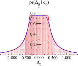
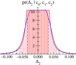
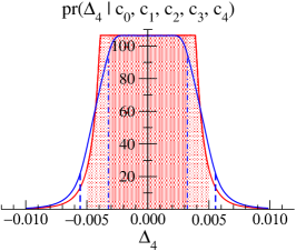
Figure 1: (color online) Posteriors for $\Delta_{k}^{(1)}$ under Set ${\rm A}_{\epsilon}^{(1)}$ priors of Table 1 for $k=0$, 2, and 4 with $Q=0.33$. In all cases, $c_{n}=1$ was assumed. The solid red curve is the analytic result from Eq. (21), with the shaded regions marking the 68% and 95% DOB intervals. The solid blue curve is the posterior $\Delta_{k}$ for ${\rm A}_{\epsilon}$ once higher-order terms are included, with dot-dashed and dashed lines marking the corresponding 68% and 95% DOB intervals.

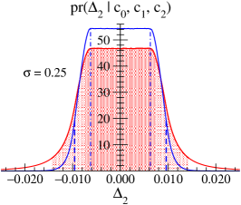
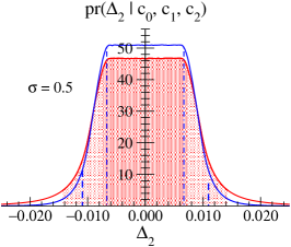
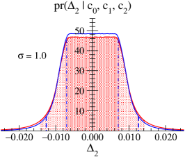
Figure 2: (color online) Comparison of $\Delta_{2}$ for prior set ${\rm A}_{\epsilon}$ (red solid line) and B (blue solid line) for $\sigma=0.25$, $0.5$ and $1.00$ respectively. In each case $c_{0},c_{1},c_{2}$ are all set to unity with an expansion parameter $Q=0.2$. The DOB intervals are indicated as in Fig. 1.

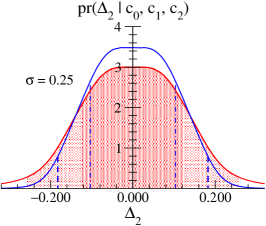
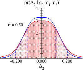
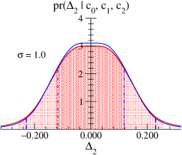
Figure 3: (color online) Comparison of $\Delta_{2}$ for prior set ${\rm A}_{\epsilon}$ (red solid line) and B (blue solid line) for three values of $\sigma$ and $c_{0},c_{1},c_{2}$ all set to unity with an expansion parameter $Q=0.5$. The DOB intervals are indicated as in Fig. 1.

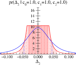
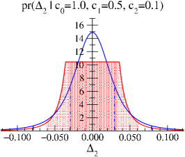
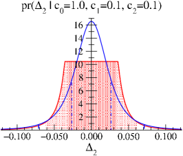
Figure 4: (color online) Comparison of $\Delta_{2}$ for prior set ${\rm A}_{\epsilon}$⁽¹⁾ (red solid line) and ${\rm C}_{\epsilon}$⁽¹⁾ (blue solid line)—note both are in the leading-omitted-term approximation—for three sets of $c_{n}$ values with an expansion parameter $Q=0.33$. These sets are (left-to-right) $\{c_{n}\}(a)\equiv\{1.0,1.0,1.0\}$, $\{c_{n}\}(b)\equiv\{1.0,0.5,0.1\}$, and $\{c_{n}\}(c)\equiv\{1.0,0.1,0.1\}$. The DOB intervals are indicated as in Fig. 1.

Before applying the Bayesian framework developed by CH, and extended above, to the specific problem of NN scattering, we make some general observations on the form of the posteriors for $\Delta_{k}$ and the systematics of the 68% and 95% DOB intervals for various prior sets from Table 1.

We start with the set ${\rm A}_{\epsilon}$, defined by $\bar{c}_{<}=\epsilon$, $\bar{c}_{>}=1/\epsilon$, with $\epsilon\rightarrow 0$ (in practice all results here in which $\epsilon$ is invoked use $\epsilon=0.001$). The posterior distribution for $\Delta_{k}^{(1)}$ in Eq. (21), which assumes the first omitted term dominates the error, has a flat central plateau with power-suppressed tails. This is illustrated by the red curves in Fig. 1 for $k=0$, $k=2$, and $k=4$, for $Q=0.33$. The heavy and light shaded regions show the 68% and 95% DOB intervals, respectively. From Eq. (25), the width of the posterior is given by $\bar{c}_{(k)}Q^{k+1}$ times a number of order unity, so the dominant effect is that the width decreases by a factor of $Q$ with each increase of $k$ by one. In fact, only the maximum value of the $c_{n}$’s for a given $k$, $\bar{c}_{(k)}$, matters under this choice of prior; the distribution of those $c_{n}$’s is irrelevant. The overall size of all DOB intervals then scales linearly with $\bar{c}_{(k)}$, so here $c_{0}$, …, $c_{k}$ have all been set to one for simplicity. For Set A priors the generalization to other cases is trivial.

To relax the first-term approximation we include the first four omitted terms in our computation of $\Delta_{k}$. The result is then converged numerically in all cases shown, so in practice Set $Y^{(4)}$ ($Y=A$, $B$, or $C$) priors lead to the same results as when arbitrarily many higher-order terms included in the truncation-error calculation. In consequence, we do not include superscripts below when reporting results with terms beyond the first omitted one included in the computation of $\Delta_{k}$. Such calculations show that the central plateau in the posterior becomes rounded (blue curve in Fig. 1). The corresponding effect on the DOB intervals depends on the value of $k$; for $k\geq 2$ there is no significant effect on the 68% DOB intervals while the 95% intervals are increased slightly.

If we use the more informative log-normal prior for $\bar{c}$ from set B, the tails are more quickly suppressed than for set ${\rm A}_{\epsilon}$, to a degree that depends in detail on the values of $\sigma$ and $Q$ Bagnaschi:2014eva ; Bagnaschi:2014wea . Representative examples for $\Delta_{2}$ are shown in Figs. 2 and 3 for $Q=0.2$ and $Q=0.5$, respectively, with $\sigma=0.25$, $0.5$, and $1.0$ respectively. We see that the 68% DOB and 95% DOB intervals are smaller that those for ${\rm A}_{\epsilon}$, with the difference increasing with smaller $\sigma$. The further extension of the tail for ${\rm A}_{\epsilon}$ is not surprising as we have allowed for the possibility of $\bar{c}$ having a large range. As $\sigma$ gets larger, the posteriors for each $Q$ value approach the ${\rm A}_{\epsilon}$ result; once $\sigma\geq 1.0$ there is very little difference between ${\rm A}_{\epsilon}$ and Set B for $k\geq 2$. $k=0$ and $k=1$ are more sensitive to $\sigma$.

Table 2: Resulting 68% and 95% DOB intervals for $\Delta_{k}$ using Set ${\rm A}^{(1)}$ with different choices for the minimum and maximum of the $\bar{c}$ prior. In all cases $\bar{c}_{(k)}=1$.

	min/max	$Q$	$k=0$	$k=1$	$k=2$	$k=3$	$k=4$
	0.001/1000		0.31	0.041	0.0073	0.00136	0.00026
	0.25/4.0	0.20	0.22	0.039	0.0072	0.00136	0.00026
	0.50/2.0		0.18	0.035	0.0068	0.00132	0.00026
	0.001/1000		0.51	0.111	0.033	0.0101	0.0032
68%	0.25/4.0	0.33	0.36	0.106	0.032	0.0101	0.0032
	0.50/2.0		0.30	0.095	0.030	0.0098	0.0031
	0.001/1000		0.78	0.26	0.113	0.053	0.026
	0.25/4.0	0.50	0.55	0.243	0.112	0.053	0.025
	0.50/2.0		0.45	0.22	0.106	0.051	0.025
	0.001/1000		1.96	0.103	0.0137	0.0023	0.00041
	0.25/4.0	0.20	0.47	0.077	0.0129	0.0022	0.00041
	0.50/2.0		0.29	0.056	0.011	0.0020	0.00039
	0.001/1000		3.2	0.28	0.0614	0.0168	0.0050
95%	0.25/4.0	0.33	0.77	0.21	0.058	0.0166	0.0050
	0.50/2.0		0.48	0.152	0.048	0.0150	0.0047
	0.001/1000		4.91	0.645	0.21	0.0884	0.040
	0.25/4.0	0.50	1.16	0.48	0.201	0.087	0.040
	0.50/2.0		0.73	0.35	0.166	0.079	0.038

We might expect that the Set B results with $\sigma>1.0$ will be even closer to those from Set A if we impose a range of $\bar{c}$ values in Set A that reflects naturalness expectations. Results of varying the range over which $\bar{c}$ is marginalized are shown in Table 2, where we compare DOB intervals for $\Delta_{k}$ with $k$ from 0 to 4. For $k\geq 3$, the change in the range of $\bar{c}$ has no noticeable effect on either the 68% or 95% DOB. For $k=2$, effects are 5–10% on the 68% interval if a narrow range ($\bar{c}$ from 0.5 to 2.0) is employed. Effects on the 95% interval can be up to 20% if this narrow range is employed at $k=2$.

Table 3: DOB intervals for Sets ${\rm A}_{\epsilon}$ and ${\rm C}_{\epsilon}$, with and without the leading omitted term approximation, for $k=2$, with three sets of $c_{n}$ values. These sets are $\{c_{n}\}(a)\equiv\{1.0,1.0,1.0\}$, $\{c_{n}\}(b)\equiv\{1.0,0.5,0.1\}$, and $\{c_{n}\}(c)\equiv\{1.0,0.1,0.1\}$.

	$Q$	${\rm A}_{\epsilon}^{(1)}/{\rm A}_{\epsilon}$	${\rm C}_{\epsilon}^{(1)}/{\rm C}_{\epsilon}\ \{c_{n}\}(a)$	${\rm C}_{\epsilon}^{(1)}/{\rm C}_{\epsilon}\ \{c_{n}\}(b)$	${\rm C}_{\epsilon}^{(1)}/{\rm C}_{\epsilon}\ \{c_{n}\}(c)$
	0.20	0.0073/0.0073	0.0095/0.0097	0.0062/0.0063	0.0056/0.0057
68%	0.33	0.033/0.033	0.043/0.045	0.028/0.029	0.025/0.026
	0.50	0.113/0.123	0.149/0.171	0.096/0.111	0.087/0.100
	0.20	0.0137/0.0137	0.025/0.026	0.017/0.017	0.015/0.015
95%	0.33	0.061/0.066	0.114/0.121	0.074/0.079	0.067/0.071
	0.50	0.21/0.25	0.40/0.46	0.26/0.30	0.23/0.27

The Set C priors are qualitatively different from Set A because they correspond to an ensemble naturalness assumption for $\text{pr}(c_{i}|\bar{c})$, which means that the distribution of $c_{n}$’s for a given $k$—and not just their maximum—affects the result. This is illustrated by the results in Table 3, in which DOB intervals for $\Delta_{2}$ with prior choices ${\rm A}_{\epsilon}$ and ${\rm C}_{\epsilon}$ are compared. Because $k=2$, the coefficients $c_{0}$, $c_{1}$, and $c_{2}$ are all influential; we consider three representative choices for their values. The systematics going from $c_{n}$ sets $a$ to $b$ to $c$ show that having more $c_{n}$’s near one leads to larger DOB intervals. Taking $c_{n}(b)$ to give generic results for a roughly even distribution of coefficients we find that the Set C vs. Set A comparison is close: only a 10-15% increase for the 68% DOB and a roughly 20% increase for the 95% DOB. (The Set A intervals are wider for all but the case in which all three known coefficients are 1.0.) This reflects the stronger central peaking of the Set C pdf under a reasonable distribution of the first three coefficients, as depicted (in the first-omitted-term approximation) in Fig. 4. Such differences in DOB intervals under different prior choices will be amplified if $k=0$ or $k=1$.

Table 3 also assesses the approximation of keeping only the leading omitted term in $\Delta_{2}$. Once $Q=0.5$ we see appreciable differences between Set ${\rm C}^{(1)}$ and Set C results that include multiple higher-order terms, but even then it is only about a 15% effect on the error bar.

III Comparison to recent chiral EFT results for np scattering

III.1 EKM’s truncation-error estimates

Chiral perturbation theory ($\chi{\rm PT}$) encodes the consequences of QCD at momenta of order the pion mass Weinberg (1979); Gasser and Leutwyler (1984); Jenkins and Manohar (1991); Bernard and Meißner (2007). It can be used to compute the interaction of single nucleons and pions for momenta well below the chiral-symmetry-breaking scale, $\Lambda_{\chi{\rm SB}}$. $\chi$PT yields a purely perturbative expansion in powers of $(p,m_{\pi})/\Lambda_{\chi{\rm SB}}$ for low-energy pion-pion and pion-nucleon scattering. But, nuclei are bound states, and will not be generated from such an expansion.

In the early 1990s Weinberg pointed out that the infrared enhancement associated with multi-nucleon intermediate states meant that the $\chi$PT expansion cannot be applied directly to the scattering amplitude in systems with more than one nucleon Weinberg (1990). He argued that the $\chi$PT Lagrangian and counting rules should instead be used to compute an NN (or NNN or …) potential up to some fixed order, $n$, in $\chi$PT. Such an expansion can then be examined for convergence with $n$. The $\chi$PT potential $V$ was computed to $O(Q^{3})$ in Refs. Ordonez et al. (1996); Epelbaum et al. (2000); Entem and Machleidt (2002), and to $O(Q^{4})$ in Refs. Entem and Machleidt (2003); Epelbaum et al. (2005). Consistent three-nucleon forces have been derived and implemented in such an approach van Kolck (1994); Epelbaum et al. (2002).

However, while there is a $\chi$PT expansion for $V$, the resulting nuclear binding energies (and other observables) contain effects to all orders in the chiral expansion: there is no obvious perturbative expansion for them. In practice, chiral EFT for few-nucleon systems is often implemented as described in the previous paragraph, but with the Hamiltonian acting only on a limited space: in momentum space a cutoff $\Lambda$ in the range $450<\Lambda<800$ MeV must be imposed Marji et al. (2013). From now on when we use the term chiral EFT in the context of few-nucleon systems we mean calculations that are carried out in this way. A formal justification of the $Q$-expansion (e.g., via the distorted-wave Born approximation evaluation of higher-order contributions Long and Yang (2012, 2011); Pavon Valderrama (2011) or use of a relativistic propagator Epelbaum and Gegelia (2012, 2013)) requires a more sophisticated power counting Nogga et al. (2005); Birse ; Phillips (2013). Nevertheless, in practice, the convergence of chiral EFT calculations for observables can be examined a posteriori to see if they inherit the $Q$-expansion that has been used for the potential.

In two recent papers, EKM estimated the errors that arise from truncation of the chiral EFT expansion at a finite order Epelbaum et al. (2015, 2014) (see also Ref. Binder et al. (2015)). Similar prescriptions have previously been used in other EFT contexts (see, e.g., Refs. Phillips et al. (2000); Griesshammer et al. (2012)). Such estimates apply to individual observables (such as the total cross section for neutron-proton scattering at a given lab energy or nucleon electric and magnetic polarizabilities). They are independent of procedures used to fit LECs to two-body scattering data at each order. While Bayesian analysis could also be applied to those procedures that is not our concern here; it will be the focus of a future publication Wesolowski et al. .

Instead, EKM assume that the EFT expansion holds for individual observables $X(p)$, i.e.,

$$X(p)=X_{0}\sum_{n=0}^{k}c_{n}(p)Q^{n}\;,$$ (31)

with $Q$ the EFT expansion parameter, and $c_{1}=0$ in the Weinberg expansion for NN scattering in chiral EFT. Cumulative sums at LO, NLO, N²LO, N³LO, and N⁴LO are then given by:

$$X^{\rm LO}(p) = c_{0}(p)\;,$$ (32)

$$X^{\rm NLO}(p) = \sum_{n=0}^{2}c_{n}(p)Q^{n}\;,$$ (33)

$$X^{\rm N^{j}LO}(p) = \sum_{n=0}^{j+1}c_{n}(p)Q^{n},\;j=2,3,4\;.$$ (34)

EKM also assume that the dominant error at order $k$ comes from the first omitted—($k+1$)^th—term. Two ingredients go into their estimate of this term. The first is to identify the EFT expansion parameter $Q$, defined as

$$Q\equiv\max\left(\frac{p}{\Lambda_{b}},\ \frac{m_{\pi}}{\Lambda_{b}}\right)\;.$$ (35)

Note that, in contrast to pQCD, this is a momentum-dependent expansion parameter, and so the expansion will perform differently at different kinematic points. Furthermore, to know $Q$ we must identify $\Lambda_{b}$, the breakdown scale of the EFT. In Refs. Epelbaum et al. (2015, 2014), EKM estimate $\Lambda_{b}$ from error plots of the fit phase shifts. The second ingredient is to determine the shift beyond N^jLO as:

$$\Delta X^{\rm N^{j}LO}=Q^{j+2}{\rm max}(|c_{0}|,|c_{1}|,\ldots,|c_{j+1}|)\;,$$ (36)

where the $c_{n}$’s are defined as above.

In Refs. Epelbaum et al. (2015, 2014) the expressions for the theory error are defined via differences of the partial sums (34), but the result may be summarized compactly according to Eq. (36). The similarity of this prescription to the simplest analytic form obtained above with ${\rm A}_{\epsilon}$⁽¹⁾ priors, the CH procedure written in Eq. (25), is evident. For a given observable, the value of $Q$ that is identified defines the perturbative expansion parameter, and the EKM uncertainty is the maximum coefficient times the first omitted power of $Q$. Up to factors of order unity, this is what Eq. (25) predicts for the 68% (“$1\sigma$”) DOB interval. There is then clearly a semi-quantitative correspondence. We now make a quantitative comparison using the various priors from Table 1.

Table 4: Order-by-order calculations for $\sigma_{np}$ in mb for $R=0.9\,$fm from EKM Epelbaum et al. (2015, 2014); Epelbaum . Lab energy $T_{\rm lab}$ and relative momentum $p_{\rm rel}$ are in units of MeV.

$T_{\rm lab}$	$p_{\rm rel}$	$\sigma_{\rm LO}$	$\sigma_{\rm NLO}$	$\sigma_{\rm N^{2}LO}$	$\sigma_{\rm N^{3}LO}$	$\sigma_{\rm N^{4}LO}$
50	153	183.6	166.5	167.0	166.8	167.5
96	212	84.8	75.1	78.3	77.5	78.0
143	259	52.5	49.1	54.2	53.7	53.9
200	307	34.9	35.9	42.6	43.2	42.7

Table 5: Order-by-order calculations for $\sigma_{np}$ in mb for $R=1.2\,$fm from EKM Epelbaum et al. (2015, 2014); Epelbaum . Lab energy $T_{\rm lab}$ and relative momentum $p_{\rm rel}$ are in units of MeV.

$T_{\rm lab}$	$p_{\rm rel}$	$\sigma_{\rm LO}$	$\sigma_{\rm NLO}$	$\sigma_{\rm N^{2}LO}$	$\sigma_{\rm N^{3}LO}$	$\sigma_{\rm N^{4}LO}$
50	153	159.4	164.8	165.6	167.2	167.9
96	212	60.2	68.9	71.3	78.1	78.5
143	259	30.8	38.6	41.4	52.6	52.7
200	307	17.2	22.5	25.0	38.6	38.3

Table 6: Dimensionless coefficients from the expansion of $\sigma_{np}=\sigma_{\rm LO}\sum_{n=0}^{5}c_{n}Q^{n}$ for $R=0.9\,$fm from Table 4, with $Q=p_{\rm rel}/600\,$MeV.

$T_{\rm lab}$	$c_{0}$	$c_{1}$	$c_{2}$	$c_{3}$	$c_{4}$	$c_{5}$
50	1.0	0.0	$-1.43$	0.16	$-0.26$	3.5
96	1.0	0.0	$-0.92$	0.86	$-0.61$	1.07
143	1.0	0.0	$-0.35$	1.21	$-0.27$	0.25
200	1.0	0.0	0.11	1.44	0.25	$-0.41$

Table 7: Dimensionless coefficients from the expansion of $\sigma_{np}=\sigma_{\rm LO}\sum_{n=0}^{5}c_{n}Q^{n}$ for $R=1.2\,$fm from Table 5, with $Q=p_{\rm rel}/400\,$MeV.

$T_{\rm lab}$	$c_{0}$	$c_{1}$	$c_{2}$	$c_{3}$	$c_{4}$	$c_{5}$
50	1.0	0.0	0.23	0.09	0.47	0.54
96	1.0	0.0	0.51	0.27	1.43	0.16
143	1.0	0.0	0.60	0.33	2.07	0.03
200	1.0	0.0	0.52	0.32	2.28	$-0.07$

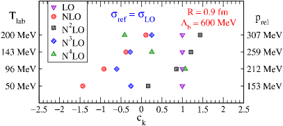
Figure 5: (color online) Chiral EFT expansion coefficients from Table 6 for $\sigma_{np}$ at four different energies using potentials with regulator parameter $R=0.9\,$fm and $\Lambda_{b}=600\,$MeV. Note that the coefficient $c_{5}=3.5$ at $T_{\rm lab}=50$ MeV is off scale.

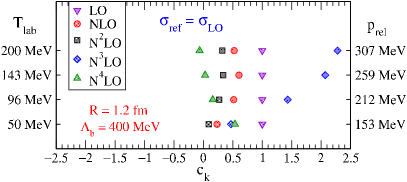
Figure 6: (color online) Chiral EFT expansion coefficients from Table 6 for $\sigma_{np}$ at four different energies using potentials with regulator parameter $R=1.2\,$fm and $\Lambda_{b}=400\,$MeV.

We note that in chiral EFT, having posited a $Q$ expansion, we do not find the coefficients directly but extract them from the calculations at different orders. In contrast, for the QCD expansions, the coefficients are calculated independently of each other. Thus the EFT application will require additional empirical verification, see Sec. IV.

III.2 The pattern of EFT coefficients in EKM’s result

In Refs. Epelbaum et al. (2015) and Epelbaum , results for the neutron-proton total cross section at various energies are given for several values of a coordinate-space regulator parameter $R$. These provide empirical tests of the priors from Table 1. The order-by-order cross sections are given in Tables 4 and 5 for $R=0.9\,$fm and $R=1.2\,$fm, respectively. In line with Eq. (1), we write the cross section at order $k$ in the chiral EFT expansion as

$$\sigma_{np}(E_{\rm lab})\approx\sigma_{\rm ref}\sum_{n=0}^{k}c_{n}\left(\frac{p}{\Lambda_{b}}\right)^{n}\;,$$ (37)

where $\sigma_{\rm ref}$ is a reference cross section that might be taken as $\sigma_{\rm LO}$, as we do here, or the ${\rm N}{}^{4}{\rm LO}$ result, or the experimental value. The analysis is not sensitive to this choice. The breakdown scale $\Lambda_{b}$ was identified in Ref. Epelbaum et al. (2015) as $\Lambda_{b}=600\,$MeV for cutoffs $R=0.8$, 0.9, and 1.0 fm, $\Lambda_{b}=500\,$MeV for $R=1.1\,$fm, and $\Lambda_{b}=400\,$MeV for $R=1.2\,$fm. Note that this decrease in $\Lambda_{b}$ with increasing $R$ corresponds to the change in the regulator cutoff scale rather than a change in the intrinsic underlying breakdown scale. In Ref. Furnstahl:2014jpg it was emphasized that residuals for a $k$th-order EFT calculation had two types of errors: regulator artifacts dictated by the imposed cutoff $\Lambda$ ($\sim 1/R$ in this context) and truncation errors in the Hamiltonian dictated by the underlying breakdown scale $\Lambda_{b}$. EKM do not make this distinction in their notation, i.e., they use $\Lambda_{b}$ for both.

Under the EKM choices for $\Lambda_{b}$, the dimensionless $c_{n}$ coefficients are given in Tables 6 and 7 and Figs. 5 and 6 for the R=0.9 fm and R=1.2 fm cases respectively. Although the coefficients in both cases are natural, rather different patterns are seen. As discussed and illustrated by EKM (e.g., see Fig. 2 of Ref. Epelbaum et al. (2014)), the softer cutoff shifts contributions between different chiral orders so that the systematic pattern of corrections is disrupted. In particular, corrections at orders ${\rm N}{}^{2}{\rm LO}$ and ${\rm N}{}^{4}{\rm LO}$, which are purely from non-analytic terms in the chiral expansion, become heavily regulated by the soft cutoff. This has the consequence that the corresponding coefficients are anomalously small—which may, in turn result in ${\rm N}{}^{3}{\rm LO}$ coefficients being somewhat large. This pattern is seen in Fig. 6, but what is shown there is insufficient to definitively establish there is an inter-order correlation due to regulator artifacts. Here we focus on the $R=0.9\,$fm example to ensure that the pattern is primarily driven by the inheritance of naturalness from the fit low-energy constants (LECs), and not by regulator artifacts that spring from a choice of $R$ that makes the $\Lambda\sim 1/R$ effects predominate over the physics at $\Lambda_{b}$ that was integrated out of the theory.

III.3 DOB intervals from a Bayesian analysis

There is a minimum of necessary information that must exist between the prior and data in order for the resulting posterior to accurately describe the above distributions. Two extremes exist: a large supply of precise and accurate data paired with an uninformative prior (or, even worse, an informative yet incorrect prior) and a small amount of data paired with a precisely and accurately defined prior. Each of these situations may result in realistic posteriors as lack of information in one realm is compensated by abundance in the other. In practice, though, we conduct analyses between these extremes. We are often able to define a reasonable, and appropriately loose, prior that is subsequently fine-tuned by a modest amount of data. We will now show that each of the priors defined in Table 1 may be considered reasonable representations of naturalness in the EFT-coefficient distribution obtained in the previous subsection. The DOB intervals that result from Bayesian analyses using these priors show agreement and increased similarity at low $Q$ and high $k$—where the strength of available data is greatest.

Table 8: DOB intervals for EKM $\sigma_{np}$ with $R=0.9\,$fm using prior Set ${\rm A}_{\epsilon}^{(1)}$.

DOB	$\mbox{E}_{\rm lab}$	$Q$	$\mbox{LO}^{\prime}$	LO	NLO	${\rm N}{}^{2}{\rm LO}$	${\rm N}{}^{3}{\rm LO}$	${\rm N}{}^{4}{\rm LO}$
68%	50	0.255	0.40	0.102	0.024	0.0055	0.0013	0.00079
$\times 183.6$ mb			73.	19.	4.4	1.0	0.24	0.15
68%	96	0.354	0.55	0.20	0.045	0.0142	0.0047	0.0017
$\times 84.8$ mb			47.	17.	3.8	1.2	0.40	0.15
68%	143	0.432	0.68	0.29	0.082	0.038	0.015	0.0064
$\times 52.5$ mb			35.	15.	4.3	2.0	0.81	0.34
68%	200	0.511	0.80	0.41	0.136	0.089	0.043	0.021
$\times 34.9$ mb			28.	14.	4.7	3.1	1.5	0.73
95%	50	0.255	2.6	0.650	0.061	0.0103	0.0022	0.0012
$\times 183.6$ mb			470	120	11.	1.9	0.40	0.23
95%	96	0.354	3.5	1.25	0.115	0.027	0.0079	0.0027
$\times 84.8$ mb			300	110	9.8	2.3	0.67	0.23
95%	143	0.432	4.3	1.87	0.21	0.072	0.026	0.010
$\times 52.5$ mb			230	98.	11.	3.8	1.4	0.53
95%	200	0.511	5.1	2.6	0.35	0.17	0.071	0.033
$\times 34.9$ mb			180	91.	12.	5.9	2.5	1.1

Table 9: DOB intervals for EKM $\sigma_{np}$ scaled by $\sigma_{\rm LO}$ with $R=0.9\,$fm. Results for prior Sets ${\rm A}_{\epsilon}$, B (with $\sigma=1.0$), and ${\rm C}_{\epsilon}$, all without the leading-omitted-term approximation.

	set	$\mbox{E}_{\rm lab}$	$Q$	$\mbox{LO}^{\prime}$	LO	NLO	${\rm N}{}^{2}{\rm LO}$	${\rm N}{}^{3}{\rm LO}$	${\rm N}{}^{4}{\rm LO}$
	${\rm A}_{\epsilon}$			0.43	0.11	0.025	0.0055	0.0013	0.00080
	${\rm C}_{\epsilon}$	50	0.255	0.48	0.12	0.028	0.0053	0.0011	0.00056
	B			0.29	0.073	0.022	0.0052	0.0013	0.00076
	${\rm A}_{\epsilon}$			0.59	0.21	0.048	0.015	0.0048	0.0018
	${\rm C}_{\epsilon}$	96	0.354	0.69	0.25	0.060	0.019	0.0058	0.0021
68%	B			0.40	0.143	0.043	0.014	0.0047	0.0017
	${\rm A}_{\epsilon}$			0.74	0.32	0.089	0.040	0.016	0.0067
	${\rm C}_{\epsilon}$	143	0.432	0.87	0.38	0.088	0.043	0.015	0.0059
	B			0.51	0.22	0.080	0.038	0.016	0.0065
	${\rm A}_{\epsilon}$			0.91	0.46	0.15	0.097	0.046	0.022
	${\rm C}_{\epsilon}$	200	0.511	1.08	0.58	0.14	0.096	0.041	0.019
	B			0.63	0.32	0.14	0.091	0.044	0.022
	${\rm A}_{\epsilon}$			2.7	0.69	0.066	0.011	0.0023	0.0013
	${\rm C}_{\epsilon}$	50	0.255	3.3	0.85	0.089	0.014	0.0027	0.0013
	B			0.67	0.172	0.042	0.0091	0.0021	0.0012
	${\rm A}_{\epsilon}$			3.8	1.3	0.13	0.030	0.0088	0.0030
	${\rm C}_{\epsilon}$	96	0.354	4.8	1.7	0.20	0.050	0.0142	0.0049
95%	B			0.97	0.34	0.088	0.026	0.0083	0.0029
	${\rm A}_{\epsilon}$			4.7	2.0	0.24	0.083	0.030	0.012
	${\rm C}_{\epsilon}$	143	0.432	6.0	2.6	0.29	0.114	0.038	0.014
	B			1.22	0.53	0.17	0.071	0.028	0.0115
	${\rm A}_{\epsilon}$			5.7	2.9	0.41	0.20	0.088	0.041
	${\rm C}_{\epsilon}$	200	0.511	7.4	3.8	0.47	0.26	0.100	0.043
	B			1.53	0.78	0.29	0.173	0.081	0.040

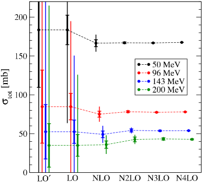
Figure 7: (color online) Cross sections at different energies and orders from EKM, with DOB intervals at each order using Set ${\rm A}_{\epsilon}$ priors. The thick error bars indicate 68% DOB intervals while the thin error bars indicate 95% DOB intervals.

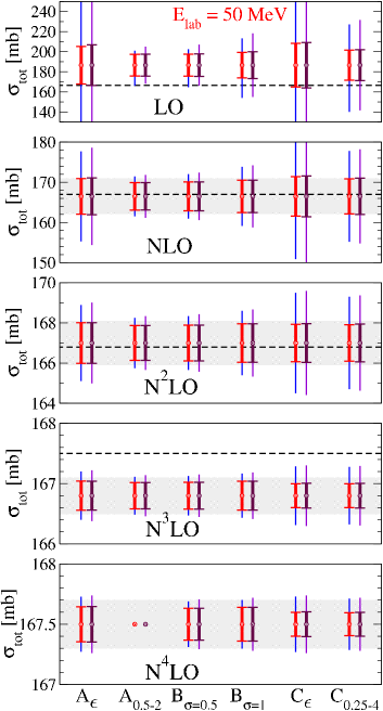
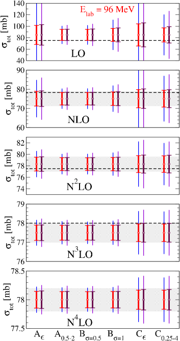
Figure 8: (color online) Cross sections at 50 MeV and 96 MeV for all orders from EKM, with DOB intervals at each order using a wide variety of prior sets. Note the change in scale at each order. The thick error bars indicate 68% DOB intervals while the thin error bars indicate 95% DOB intervals. In each panel the dashed line is the result of the next-order calculation (NLO at LO, N²LO at NLO, etc.), shown to facilitate an assessment of the statistical consistency of different prior choices. For each prior choice, the intervals on the left are from keeping only the first omitted term while those on the right are including four omitted terms. The shaded bands indicate the uncertainty from EKM.

Figure 9: (color online) Cross sections at 143 MeV and 200 MeV for all orders from EKM, with DOB intervals at each order using a wide variety of sets. Note the change in scale at each order.The thick error bars indicate 68% DOB intervals while the thin error bars indicate 95% DOB intervals. In each panel the dashed line is the result of the next-order calculation (NLO at LO, N²LO at NLO, etc.), shown to facilitate an assessment of the statistical consistency of different prior choices. For each prior choice, the intervals on the left are from keeping only the first omitted term while those on the right are including four omitted terms. The shaded bands indicate the uncertainty from EKM.

In Fig. 7, cross sections from Table 4 for $R=0.9\,$fm at four different energies are plotted order-by-order in the chiral expansion, with error bars indicating the 68% and 95% DOB intervals if we adopt prior set ${\rm A}_{\epsilon}$. The $\mbox{LO}^{\prime}$ error bars are from the calculation for the posterior of $\Delta_{0}$ while the LO error bars are from the posterior of $\Delta_{1}$. When calculating $\Delta_{1}$ we have $k=1$ and $n_{c}=1$, so the resulting error bar is simply $Q$ times the $\mbox{LO}^{\prime}$ one. This is the correct error estimate for a LO chiral EFT calculation of NN scattering, as long as we know a priori that the coefficient $c_{1}$ in the expansion (37) is identically zero.

Cross sections at subsequent orders generally fall within the DOB intervals of lower-order error analyses—in accord with the DOB intervals’ statistical interpretation. The order-by-order decrease in the error bars primarily reflects the additional factors of $Q$ with each successive order. The very conservative assumption for $\text{pr}(\bar{c})$ used here, which encodes ignorance of its scale even though we anticipate naturalness, leads to long tails in the posterior for the lowest orders and correspondingly large 95% DOB intervals— further reflecting the non-Gaussian nature of this distribution. When we use a form for $\text{pr}(\bar{c})$ that reflects the expectation of naturalness, the long tails are suppressed and the 95% DOB intervals are closer to “$2\sigma$” errors, although the pdfs do remain non-Gaussian in general.

Table 8 is an analytical compilation of DOB intervals in the limiting case of ${\rm A}_{\epsilon}$ with the leading-term approximation, see Eq. (25). The top number in each cell has been calculated using coefficients of Table 6, which are scaled with the $\sigma_{\rm ref}$ corresponding to each energy. The lower number is the resulting DOB interval in units of mb with the factor of $\sigma_{\rm ref}=\sigma_{\rm LO}$ included. The 95% DOB interval being more than 6 times broader than the corresponding 68% DOB interval at $\mbox{LO}^{\prime}$ and LO emphasizes the strength of tails within these posteriors.

Representative numerical results for the various prior sets are given in Table 9. Though we omit mention of $\sigma_{\rm ref}$, values here should also be multiplied by the energy-appropriate $\sigma_{\rm ref}$ (i.e., $\sigma_{\rm LO}$) to obtain DOB values in units of mb. Systematically, we observe that the ratios of DOB intervals between prior sets are the same across all 4 energies for $\mbox{LO}^{\prime}$ and LO as all $c_{1}$’s are 0 and we have scaled all $c_{0}$’s to the value 1.0. Thus, given the same set of coefficients, all posteriors scale similarly with energy. Table 9 also shows that the ensemble prior in Set ${\rm C}_{\epsilon}$ generally predicts 68% DOB intervals quite similar to those from Set ${\rm A}_{\epsilon}$, with much greater variation for 95% DOB intervals for the lower orders. From this, we see that prior choice affects the structure of the tails more significantly than the structure of the peak. This is indicative of the strength of information coming from the data and the prior at different points in the distribution. Though Set B results in significantly narrower DOB intervals at low $k$, the EFT coefficients provide enough information for $k\geq 2$ to modify these posteriors into agreement with those of Sets ${\rm C}_{\epsilon}$ and ${\rm A}_{\epsilon}$.

A comparison of Set A results in Table 9 with those in Table 8 shows that the approximation of keeping only the leading omitted term is excellent for the 68% DOB for $k>2$ and still quite good for $k=1$ (which is the true leading order). This approximation always underestimates the interval from including higher-order terms and worsens as the expansion parameter $Q$ increases. Figures 8 and 9 show that this result is general and that the approximation is better for the 95% interval with a less conservative prior for $\bar{c}$. One outlier is the $k=5$ prediction at $T_{\rm lab}=50\,$MeV where we see consequences of a $c_{5}$ coefficient known to have an anomalously large value, which is an artifact of the fitting procedure Epelbaum . Note that this results in the omission of the DOB interval for ${\rm N}{}^{4}{\rm LO}$ at 50 MeV with Set $A_{0.5-2}$ as $\bar{c}_{>}$ is then less than $\bar{c}_{(k)}$, so the distribution is not defined in this case.

Overall, the prior sets ${\rm A}_{\epsilon}$ and ${\rm C}_{\epsilon}$ appear to be too conservative for predictions at LO; we know that ${\rm A}_{\epsilon}$ and ${\rm C}_{\epsilon}$ have incorporated less information than the alternatives so it is no surprise that their posteriors are more widely distributed. Importantly, we find that the posteriors for $\Delta_{k}$ for $k\geq 2$ are largely insensitive to the choice of prior, even for the 95% DOB interval. As posteriors retain artifacts of the prior in inverse proportion to the strength of the data, this similarity suggests that the data is sufficiently informative that any reasonable prior is properly subservient and thus able to adapt to evidence of the real world presented by the data.

IV Choice of expansion parameter

In the previous section, the scale $\Lambda_{b}$ in the expansion parameter was taken from Ref. Epelbaum et al. (2015), where it was extracted from error plots after the fit of the LECs. This identification was certainly not rigorous in any statistical sense. Therefore here we explore how $\Lambda_{b}$ can be extracted from the convergence pattern of the EFT for observables.

In the case of pQCD, Cacciari and Houdeau discussed using an expansion parameter that is different from $\alpha_{s}$. They introduced a scale factor $\lambda$, so that the expansion is in powers of $\alpha_{s}/\lambda$ Cacciari and Houdeau (2011). This changes the expressions for $\text{pr}(\Delta_{k}|c_{0}\ldots,c_{k})$ by a rescaling of the expansion parameter $Q$ and a corresponding rescaling of the coefficients themselves. We can rewrite the series for an observable $X$ in terms of the rescaled expansion parameter and coefficients as

$$X=X_{0}\sum_{n=0}^{\infty}(c_{n}\lambda^{n})\times\left(\frac{Q}{\lambda}\right)^{n}\;.$$ (38)

In an EFT expansion this is equivalent to a rescaling of $\Lambda_{b}$ by a factor $\lambda$.

Subsequent papers explored procedures for determining the value of $\lambda$ based on various criteria:

• In Refs. Bagnaschi:2014eva ; Bagnaschi:2014wea , $\lambda$ was chosen empirically by comparing the consistency of the computed DOB intervals with known higher-order calculations. An extra factor of $(n-1)!$ was also introduced along with $\lambda$ in Eq. (38)—motivated by effects from renormalon chains at higher orders in the expansion. The authors denoted the resulting scheme $\overline{\rm CH}$. We have no evidence for such a factorial in our EFT expansions and do not consider it further here.

• In Ref. Forte et al. (2014), it was proposed that with the best expansion parameter, the coefficients should form a normal distribution of mean $\mu$ and standard deviation $\sigma$. This criterion was used to choose a value of $\lambda$. This approach is consistent with naturalness for the $\{c_{n}\}$, as long as $\mu$ and $\sigma$ are both $\mathcal{O}(1)$.

Here we explore these procedures for tuning the expansion parameter in the EKM cross sections, and we also suggest another criterion for assessing $\lambda$ based on the assumption of naturalness in the EFT expansion for a particular value of $\Lambda_{b}$. If a $\lambda$ emerges from such analyses that is measurably different from one, it suggests that the true breakdown scale of the EFT expansion is not $\Lambda_{b}$, but instead $\Lambda_{b}\lambda$. Given the limited number of coefficients (20 at most) at our disposal from the EKM analysis, any statistical procedure can only determine $\lambda$, and hence $\Lambda_{b}$, within sizable error bars. Our goal in this section is less to determine $\Lambda_{b}$, than to establish whether the choice $\Lambda_{b}=600$ MeV is consistent with our other a priori assumptions and deductions about the convergence properties of the EFT.

IV.1 Consistency checks based on higher-order calculations

In Refs. Bagnaschi:2014eva ; Bagnaschi:2014wea $\lambda$ was determined by checking the consistency of $\overline{\rm CH}$ DOB intervals obtained with expansion parameters $\alpha_{s}/\lambda$ in several large sets of pQCD observables. This is done by examining actual vs. expected success rates of the pQCD calculations. As stated in Ref. Jenniches (2015): “For a finite set of observables and a given model (with fixed parameters) at order $k$, the success rate is defined as the number of observables whose subsequent-order contributions are within the uncertainty interval predicted by the model.”

We want to use the observed success rates $n(p)/N$ for our EFT calculation to infer the likelihood that $p$ is the true success rate—for many different choices of $p$. If each observable being considered is uncorrelated, the success rate should follow a binomial distribution. Therefore the likelihood for $n$ successes amongst $N$ observables, given $p$, is

$$\text{pr}(n|p,N)=\frac{N!}{n!(N-n)!}p^{n}(1-p)^{N-n}\;.$$ (39)

We generalize the pdf (39) to its continuous version, the $\beta$-distribution:

$$\text{pr}(a,b|p,N)=\frac{(a+b-1)!}{(a-1)!(b-1)!}p^{a-1}(1-p)^{b-1}\;,$$ (40)

with $a=n+1$ and $b=N-n+1$. We can then compute confidence intervals (CIs) on $n$ (or, equivalently $a$) for a given value of $p$ (in practice we will consider only the 68% and 95% CIs). This can be done using standard integrals, and the result expressed in terms of a range of success rates that are consistent with the chosen value of $p$.

As in Refs. Bagnaschi:2014eva ; Bagnaschi:2014wea , we have calculations of the cross sections at several orders and energies and are trying to determine values of $\lambda$ that result in consistency between assumed values of $p$ and the resulting success rates $n$. To do this, we take the set of 16 observables we have from the EKM results: calculations at LO, NLO, N²LO, N³LO for four different lab energies. (Note that each observable must have a higher-order result to which it can be compared.) We then pick a value of $\lambda$ and proceed to assess the consistency of the success rates of the theory predictions for that $\lambda$ via this algorithm (adapted from pQCD to EFT for our purposes):

1. Select a grid of $p\%$ DOB intervals with $p$ ranging from 0 to 100.

2. Use the formalism laid out in Sections II and III to compute the $p\%$ DOB interval for each observable in the set.

3. For each next-order calculation that is within the DOB interval of the previous order, count one success.

4. Take the number of successes and divide by the total number of observables to get the actual success rate.

5. Compare the actual success rate for this value of $p$ with the 68% and 95% confidence intervals for the number of successes if $p$ were the true success rate, as computed from the distribution (40).

This algorithm generates a function of $p$ for this value of $\lambda$. If the curve is within the $68\%$ CI for the entire range of $p$ values we say that the value of $\lambda$ is consistent at $1\sigma$ with the performance of the perturbative series. Moderate fluctuations outside the $1\sigma$ band over limited regions of the entire $p$ domain can indicate a statistically consistent choice for $\lambda$, but the concern is with curves that end up systematically outside the $1\sigma$ region. This can occur in one of two ways. If the curve starts to veer above the $1\sigma$ region then that indicates the EFT predictions are too successful. The expansion parameter is overestimated, which means the EFT breakdown scale is underestimated. Alternatively, the function $n(p)/N$ may deviate well below the 68% CI, in which case the EFT is under-performing compared to statistical expectations. In that case the stated expansion parameter is too small, i.e., $\Lambda_{b}$ is overestimated. We note that this interpretation is somewhat specific to EFT: in a case where we were confident of the expansion parameter in the series we could instead use this diagnostic to probe whether different prior choices are too conservative or too aggressive.

Here though, we try to draw conclusions on the performance of the EFT expansion that are invariant under the choice of priors defined above. We thus implement this procedure for two different prior assumptions on $\bar{c}$ and the coefficients $\{c_{n}\}$. In each case we use the approximation that the leading term dominates for computational ease. The curves do not change substantially if we go beyond the first-omitted-term approximation.

We first consider Set ${\rm A}_{\epsilon}^{(1)}$. The results of computing $p\%$ success rates for various values of $\lambda$ are shown by the lines in Fig. 10. We include $68\%$ and $95\%$ confidence bands to evaluate which $\lambda$ curves meet our consistency criterion. With only 16 observables, the confidence bands are fairly wide, but still the only curve which falls completely within the $68\%$ interval is $\lambda=1.3$. The original expansion parameter at $\lambda=1$ spends some time above the $1\sigma$ region, which may reflect that DOB intervals resulting from this prior are too conservative; i.e., the actual success rate regularly exceeds the DOB that has been assigned. This is consistent with our earlier observation that Set ${\rm A}_{\epsilon}$ priors produce overly conservative DOB intervals.

We also compute the intervals using Set ${\rm C}_{\epsilon}^{(1)}$, which accounts for the effects of each coefficient and is less conservative. The results are contained in Fig. 11. We see that even for these assumptions, the $\lambda=1$ curve gets outside the $1\sigma$ band. The plot suggests $\lambda=1.1$ is a more consistent choice (other values near $\lambda=1.1$ will, of course, also be consistent). Because the DOB intervals computed with Set ${\rm C}_{\epsilon}^{(1)}$ priors are more informed by the available coefficients, this result may suggest a small increase in the assigned breakdown scale is appropriate. However, we note the small amount of data on EFT convergence that is being used here; almost all rescalings considered are consistent at the 2$\sigma$ level. Such determinations of $\Lambda_{b}$ from success rates can be sharpened by considering the behavior of the EFT series for more observables.

Figure 10: (color online) Empirical determination of $\lambda$ by comparing results at different orders. The cross sections used are the computations with the $R=0.9\,$fm regulator. Priors are Set A${}_{\epsilon}^{(1)}$. For full explanation see text.

Figure 11: (color online) Empirical determination of $\lambda$ by comparing results at different orders. The cross sections used are the computations with the $R=0.9\,$fm regulator. Priors are Set C${}_{\epsilon}^{(1)}$. For full explanation see text.

IV.2 Gaussian naturalness and the Forte method

in Ref. Forte et al. (2014), Forte et al. suggest that, for QCD expansions, the best $\lambda$ is the one that makes all the expansion coefficients closest to the same size, which they interpret as a statement that the coefficients should be normally distributed around a single number $\mu$ with variance $\sigma^{2}$ Forte et al. (2014). For a quantity for which the known information is a mean and standard deviation, in this case a particular coefficient $c_{n}$, the method of maximum entropy results in a distribution that is a gaussian Gull (1998); Sivia and Skilling (2006):

$$\text{pr}(c_{n}|\lambda,\mu,\sigma)=\frac{1}{\sqrt{2\pi}\sigma}\exp\left(-\frac{(|c_{n}|\lambda^{n}-\mu)^{2}}{2\sigma^{2}}\right)\;.$$ (41)

If we have several known coefficients, all of which are drawn from a distribution with the same mean and standard deviation, the joint pdf $\text{pr}(c_{0},\ldots,c_{k}|\lambda,\mu,\sigma)$ becomes the standard likelihood function. If $\sigma=\bar{c}$ and $\mu=0$ such a distribution corresponds to the Set C prior of Table 1.

Forte et al. consider the probability distribution for both $\mu$ and $\lambda$ given a set of $\{c_{n}\}$ Forte et al. (2014). This can be obtained from (41) using Bayes’ theorem:

$$\text{pr}(\lambda,\mu|c_{0},\ldots,c_{k},\sigma)=\frac{\text{pr}(c_{0},\ldots,c_{k}|\lambda,\mu,\sigma)\,\text{pr}(\lambda,\mu|\sigma)}{\text{pr}(c_{0},\ldots,c_{k}|\sigma)}\;.$$ (42)

Forte et al. assign no prior information to $\lambda$ and $\mu$ other than that both are larger than zero, and neither quantity depends on $\sigma$ a priori. They then take the prior and the evidence in the denominator to be an overall normalization factor that is independent of $\lambda$ and $\mu$, and so do not calculate them explicitly (cf. discussion of a scale-invariant prior for $\lambda$ below). The pdf for $\lambda$ and $\mu$ can then be written

$$\text{pr}(\lambda,\mu|c_{0},\ldots,c_{k},\sigma)\propto\text{pr}(c_{0},\ldots,c_{k}|\lambda,\mu,\sigma)\;,$$ (43)

meaning that maximizing the probability of $\lambda$ and $\mu$ is equivalent to minimizing

$$\chi^{2}=\sum_{i=1}^{N_{O}}\sum_{n=0}^{k}\left(\frac{|c_{n}^{(i)}|\lambda^{n}-\mu}{\sigma}\right)^{2}\;,$$ (44)

where $\{c_{n}^{(i)}\}$ is the set of EFT coefficients found for the $i$th observable, and $N_{O}$ is the number of observables being used to form the $\chi^{2}$. In our case $N_{O}=4$: the cross sections at the four different energies analyzed by EKM . Note also that for chiral EFT for NN scattering the coefficient $c_{1}$ is known to be zero, and so the $n=1$ term should be omitted from the sum.

The assumption that $\lambda$ has a uniform prior is not consistent with arguments regarding the invariance of the pdf under a change of scale Jeffreys (1939). In fact, $\lambda$ should be treated as a scale parameter. So, in contrast to Ref. Forte et al. (2014), we assign a uniform prior to the logarithm of $\lambda$, resulting in a probability distribution for $\lambda$ and $\mu$ that is:

$$\text{pr}(\lambda,\mu|c_{0},\ldots,c_{k},\sigma)\propto\frac{1}{\lambda}\times e^{-\chi^{2}/2}\;,$$ (45)

with the parameter space for $\lambda$ and $\mu$ restricted to both being positive. Assuming $\sigma=1$, we find the maximum of the probability (43) for the $R=0.9\,$ fm EKM coefficients occurs at $\lambda=0.92$, $\mu=0.69$. To consider the pdf of $\lambda$ only, we marginalize over the parameter $\mu$ and maximize $\text{pr}(\lambda|c_{0},\ldots,c_{k},\sigma)$ to find $\lambda=1.01^{+0.18}_{-0.19}$, which is consistent with the Forte et al. hypothesis at a 68% DOB. Larger $\sigma$’s generate still wider ranges. From this point of view too, then, $\Lambda_{b}=600$ MeV is a consistent choice for the $R=0.9$ fm np scattering EFT-expansion coefficients.

IV.3 $\chi^{2}$ test

Alternatively, we can demand that the mean of the $c_{n}$’s be fixed at $\mu=0$ and that the width $\sigma$ should affect the results as in Set C gaussian pdfs on the coefficients, where $\bar{c}$ is an important feature of the prior. This leaves us with the probability

$$\text{pr}(\lambda,\mu=0|c_{0},\ldots,c_{k},\sigma)\propto\frac{1}{\lambda}\exp\left(-\frac{\chi^{2}(\mu=0)}{2}\right)\;,$$ (46)

where $\chi^{2}(\mu=0)$ is given by Eq. (44) with $\mu=0$.

We can then test whether, for a given $\lambda$, the data, i.e., the EKM coefficients from their $R=0.9$ fm calculation, follows a normal distribution with mean zero and width $\sigma$. We do this by comparing $\chi^{2}(\mu=0)$ with the way that $\chi^{2}$ should be distributed for a normal distribution with $19$ degrees of freedom.Once again, in order to do this we must fix $\sigma$. With the choice $\sigma=1$ we find $\lambda=1.09$ gives $\chi^{2}$ of 19—the central value one would expect for this many data points . Using the rule of thumb for large number of degrees of freedom, $N$, Press et al. (1992) that the $\chi^{2}$ should have a width of $\sqrt{2N}$ indicates that $\lambda$ could (68% DOB) be anywhere between 1.01 and 1.15. As in the previous subsection, choices of $\sigma>1$ will increase this range of possibilities.

IV.4 Summary of expansion-parameter checks

In any case, while none of these methods provide a crisp result for $\Lambda_{b}$ from the 19 data points analyzed, it is reassuring that there is little evidence for a large change in $\Lambda_{b}$. Minimally, EKM’s estimate $\Lambda_{b}\approx 600\,$MeV for their $R=0.9\,$fm calculation is consistent with these analyses, and the breakdown scale may in fact be a little higher. Further investigations employing these techniques with EFT coefficients drawn from many more observables will provide more definitive answers.

V Summary and outlook

We have adapted and extended the Bayesian framework originally introduced in the context of pQCD by Cacciari and Houdeau Cacciari and Houdeau (2011) to evaluate truncation errors in EFT expansions. Assumptions about the nature of the coefficients in the expansion are encoded as priors on the coefficients of higher-order terms in the EFT series. The pdfs for these coefficients then ultimately also include information on the distribution of coefficients at orders that are calculated. Here we employed priors derived from the notion of “naturalness” of EFT coefficients, i.e., the idea that they should be $\mathcal{O}(1)$ when the observable and the momentum of the process in question are measured in appropriate units. We took the coefficients in the EFT expansion of cross sections to be natural in this sense. Such a choice is uncontroversial for perturbative processes, e.g., meson-meson scattering at momenta well below the chiral-symmetry-breaking scale. It remains to be fully investigated for cross sections in nucleon-nucleon scattering, where the relationship between the underlying scales and observables is quite complex; we rely here on an empirical validation (see Fig. 5).

We investigated the influence of two prior pdfs for EFT coefficients on the truncation errors. The first was the CH characterization of an upper bound $\bar{c}$, the second was a Gaussian of width $\bar{c}$. We also investigated the influence of priors on $\bar{c}$ itself on the results. We did this in the context of representative examples in Section II and, in Section III, using results from the order-by-order calculations of neutron-proton cross sections by Epelbaum, Krebs, and Meißner (EKM) in Ref. Epelbaum et al. (2014) (obtained with a regulator parameter $R=0.9\,$fm). Combining the insights from both sections we find:

• Priors that reflect a natural size for $\bar{c}$ give similar degree-of-belief (DOB) intervals at the lowest orders.

• The resulting error bands are tighter than those for which the scale of $\bar{c}$ is not constrained.

• For higher orders, 68% DOB intervals show little dependence on prior choice; 95% DOB intervals have larger, but still quite small, dependence.

These results have wide applicability to observables—they can be used in many EFT contexts. In the case of neutron-proton scattering our formulas provide a statistical interpretation to error bars obtained by EKM in Ref. Epelbaum et al. (2015). Their error bar is obtained in the case that the distribution of coefficients is uniform, in which case it is a $j/(j+1)*100\%$ DOB interval for the omitted terms in a N^jLO calculation. But, as already stated, truncation errors in these calculations at NLO or beyond (i.e., which include at least two orders beyond leading) were only mildly dependent on prior choice. In particular, the 68% DOB intervals obtained in our Bayesian framework varied by at most 15% amongst all the priors considered here, and the variation was less than that in calculations beyond NLO. Error bands at a given order were also consistent with a statistical interpretation when compared with known higher-order results. Truncation errors at leading order are sensitive to prior choice, since–given the choice of scaling observable we made—almost no information on the pattern of coefficients emerges from a leading-order calculation. Comparison of the resulting error band with the known results of NLO, N²LO, N³LO, and N⁴LO calculations suggests that the CH choice of a $\theta$-function distribution for coefficients, and a scale-independent distribution for the width of that $\theta$-function, is too conservative—at least for this case. Overall then, at sufficiently high order, the prior picked from Table 1 hardly matters—in practice $k=2$ may be enough. At lower orders priors provide a rigorous way to explore different assumptions about the pattern of coefficients in the EFT.

Indeed, the application of Bayesian methods to data is often criticized because of the apparently subjective selection of prior pdfs. However, the priors manifest what would otherwise be implicit assumptions, so that they can be tested. The information encoded in those assumptions is then modified in light of subsequent data: in this case the distribution of low-order coefficients influences the distributions computed for coefficients that enter the assessment of the truncation error. Furthermore, the development of specific pdfs for those higher-order coefficients allows a statistical interpretation of the “theory error”—or at least the part of it that results from the truncation of the EFT series. This allows crisp answers to questions regarding, for example, how theory error bars should be combined, or the extent to which theory errors on different quantities are correlated. Those answers may have some sensitivity to the choice of prior on the higher-order coefficients, but the advantage of the Bayesian framework is that the consequences of prior assumptions about the distribution of coefficients (Uniformly distributed or Gaussian? Natural or Scale-less?) can be traced through to the statistical uncertainties on the EFT calculation. Those assumptions can then—if necessary—be refined.

Such refinement may be necessary in light of the need to identify an EFT breakdown scale before extracting the (supposedly) $\mathcal{O}(1)$ coefficients which are input to our analysis. Mis-identification of the breakdown scale is one manner in which a particular prior could fail. But, in this case, we showed in Sec. IV that this breakdown scale $\Lambda_{b}=600$ MeV leads to success rates taken from the EFT predictions at four different energies, and for four different orders, that are statistically consistent with the DOB intervals resulting from our Bayesian formalism. Furthermore, the distribution of coefficients with the $R=0.9$ fm regulator choice is consistent with a Gaussian distribution. Qualitatively a natural distribution is not seen for the coefficients obtained using a second, larger, value of $R$. The calculation at this larger regulator radius reflects cutoff artifacts, which leads to peculiar convergence of the EFT expansion. The breakdown of the EFT is then not set by $\Lambda_{b}$, but by the effects of this softer cutoff. With the general formalism for probability distributions of EFT coefficients laid out here it will be important to check when the EFT coefficients obtained over a wide range of cutoff values and observables are empirically consistent with the application of naturalness priors to observables in the NN system.

The Bayesian approach to error estimation presented here is an alternative to procedures that calculate error bands based on variation of the EFT regulator, which could be a cutoff in either momentum or coordinate space. While variation with regulator scale gives a lower bound on the uncertainty (theories should, after all, be regulator invariant up to higher-order terms) the resulting error band has no statistical interpretation. A particular flaw is the arbitrariness of the interval in which the cutoff is varied; for QCD this is only of mild concern, because the dependence on the regulator parameter is only logarithmic. But running in the chiral EFT applied to NN scattering is much faster: it can contain high positive powers of the regulator (momentum) scale. This concern is exacerbated by the narrow range that is possible before encountering irremediable cutoff artifacts or spurious deep bound states. It is also the case that residual cutoff dependence only reflects the contribution from omitted contact operators. These only enter the chiral expansion for NN observables at even orders, and so examination of cutoff dependence alone may substantially underestimate the EFT truncation error. More generally, when computed using only cutoff variation, the error bands for predictions of observables (as opposed to quantities used to fit EFT LECs) generically exhibit undesirable systematics (e.g., sometimes growing wider with order) and often underestimate the error when compared with actual higher-order calculations Furnstahl:2014jpg . In contrast, the Bayesian assessment of truncation errors laid out here is applicable to all EFTs, admits a statistical interpretation of truncation errors, is justified when regulator parameters cannot be varied widely, and predicts decreased errors at all orders—not just when new LECs are added.

The truncation-error assessment described here is just one piece of a broader framework for EFT uncertainty quantification using Bayesian methods. We have under development analogous procedures, together with a suite of diagnostic tools, for parameter estimation and the assessment and propagation of errors—both statistical and truncation—in fitted LECs and predicted observables. Bayesian model selection is also well suited for addressing fundamental questions in nuclear EFT, such as the comparative efficacy of theories with different degrees of freedom, from pionless to chiral EFTs with and without an explicit $\Delta(1232)$.