Localized exciton-polariton modes in dye-doped nanospheres: a quantum approach

Abstract

We model a dye-doped polymeric nanosphere as an ensemble of quantum emitters and use it to investigate the localized exciton-polaritons supported by such a nanosphere. By determining the time evolution of the density matrix of the collective system, we explore how an incident laser field may cause transient optical field enhancement close to the surface of such nanoparticles. Our results provide further evidence that excitonic materials can be used to good effect in nanophotonics.

Keywords: Optical field enhancement, J-aggregate, Exciton, Permittivity, Nanophotonics, Frenkel exciton

1 Introduction

Plasmonic nanoparticles exhibit optical field enhancement when localized surface plasmon polariton (SPP) resonances are excited [1, 2]. The strength of the enhancement depends sensitively on the nanoparticle’s environment and geometry [3]. The enhancement is a vital part of phenomena such as surface-enhanced Raman scattering [4], and finds application in areas such as biosensing [5], monitoring lipid membranes [6], modifying molecular fluorescence [7] and materials characterization [8]. Localized SPP resonances occur because of the way the free conduction electrons in metal particles respond to light. For many metals at optical frequencies their response is such that the permittivity is negative - a critical requirement if the nanoparticle is to support a plasmon mode.

However, metals are not the only materials to exhibit negative permittivity; materials doped with excitonic organic dye molecules are of interest for photonics [9] and may also possess negative permittivity over a small frequency range [10]. Interest in such materials as a means to support surface exciton-polariton (SEP) resonances has recently been rekindled [11, 12, 13]. An example of this class of material is a polymer doped with dye molecules. In a previous work we showed, through experiment and with the aid of a classical model, that polyvinyl alcohol (PVA) doped with TDBC molecules (5,6-dichloro-2-[[5,6-dichloro-1-ethyl-3-(4-sulphobutyl)-benzimidazol-2-ylidene]-propenyl]-1-ethyl-3-(4-sulphobutyl)-benzimidazolium hydroxide, sodium salt, inner salt) may support localized surface exciton-polariton modes. We extracted the complex permittivity $\varepsilon(\omega)$ of this material from reflectance and transmittance measurements of thin films using a Fresnel approach [14]. TDBC was chosen because of its tendency to form J-aggregates: this leads to a narrowing of the optical resonance, making them interesting for strong coupling [15, 16, 17]. More importantly in the present context, at sufficiently high concentrations materials doped with such molecules exhibit a negative permittivity; it is this negative permittivity that enables these materials to support localized resonances. In our previous work [12] a two-oscillator Lorentz model [18, 19] was used to calculate the electric field enhancement and field confinement around the nanoparticle supporting the resonance by use of Mie theory [20, 21]. The field enhancement and confinement we predicted compared favorably with respect to gold nanospheres, albeit over a much narrower spectral range. Here we extend that earlier work by going beyond a simple classical Lorentz oscillator model. In doing so, we are able to explore new transient phenomena and develop a richer microscopic physical picture for the system.

In what follows we first outline the elements and assumptions of the quantum model we have used. We then compute the relative permittivity, $\varepsilon(\omega)$, using this model and compare our results with those obtained from a classical model. We next use our model to investigate the steady-state response of nanospheres of possessing this relative permittivity, with a focus on the nature of the localized surface exciton-polariton (LSEP) mode. The response of the same particle to a suddenly turned on applied optical field is then explored, and the occurrence of transient LSEP modes discussed.

2 Theory

The key difference between the work we report here and previous work based on a bulk, macroscopic approach [12] is that here we develop an effective medium description from a quantum model of the relative permittivity $\varepsilon=1+\chi$, where $\chi$ is the susceptibility. To do so we assume that the molecules in our material can be represented as an ensemble of two-level quantum systems. For a general material, an applied electric field $\bi{E}$ induces a polarization in the material $\bi{P}\propto{\langle\bi{d}\rangle}$, where $\langle\bi{d}\rangle$ is the average dipole moment of each molecule (quantum system). Assuming linearity, $\bi{P}$ is a linear function [22] of $\bi{E}$, given by:

$$\bi{P}=\frac{1}{2}\varepsilon_{0}\bi{E}(\chi e^{-i\omega t}+\chi^{*}e^{i\omega t})=N\langle\bi{d}\rangle$$ (1)

where $N$ is the number density of quantum emitters, and $\bi{E}$ and $\bi{d}$ are generally time and frequency dependent. To find $\chi$ and hence $\varepsilon$ we need to find $\langle\bi{d}\rangle$. If we adopt a quantum picture, then $\langle\bi{d}\rangle$ becomes the expectation value of the dipole moment and can be computed from the trace of $\rho\bi{d}$, where $\rho$ is the density matrix of the system and $\bi{d}$ is the transition dipole matrix. The density operator $\hat{\rho}$ is defined as $\hat{\rho}=\sum_{k}p_{k}|k\rangle\langle k|$, where $p_{k}$ are the relative probabilities of finding a system element in state $|k\rangle$. In order to find $\rho$, a Hamiltonian that describes the system must be determined. In general, the Hamiltonian for an open quantum system can be expressed as [23, 24],

$$\hat{H}=\hat{H}_{0}+\hat{H}_{B}+\hat{H}_{I},$$ (2)

where $\hat{H}_{0}$ is the Hamiltonian of the isolated system, $\hat{H}_{B}$ describes the interaction of $\hat{H}_{0}$ with the bath, and $\hat{H}_{I}$ describes the interaction of $\hat{H}_{0}$ with the applied electric field.

For TDBC molecules in a PVA host medium, $\hat{H}_{B}$ should represent the $3n_{m}-6=129$ intramolecular [25] vibrational modes (where $n_{m}$ is the number of atoms per molecule) with a multitude of intermolecular modes. These vibrational modes are responsible for induced decay and dephasing in the system [26, 27], along with a small shift in the excited state energy of the molecules [28]. Rather than determining $\hat{H}_{B}$ directly we have made a commonly-used simplification, that of incorporating the effects of the bath (vibrationally induced decay and dephasing) phenomenologically by application of the dissipative Lindblad superoperator (see below) and by making the assumption that the small energy shift can be ignored [23, 24, 29].

For an ensemble of $n$ two-level emitters (molecules), $\hat{H}_{0}$ can be written as [30, 28, 31],

$$\hat{H}_{0}=\hbar\omega_{0}|0\rangle\langle 0|+\sum_{i=1}^{n}\left(\hbar\omega^{(1)}_{1}|1_{i}\rangle\langle 1_{i}|+\mathop{\sum_{j=1}^{n}}_{j\neq i}J_{ij}|1_{i}\rangle\langle 1_{j}|\right),$$ (3)

where $|0\rangle$ is the ground state of the nanoparticle, and $|1_{i}\rangle$ represents a single exciton excited in the nanoparticle, localized on molecule $i$, with the other molecules in their ground states i.e. $|1_{i}\rangle=|0_{1},...,1_{i},...0_{n}\rangle$. In this way, only a single exciton is permitted within the ensemble at any time. The first term in brackets in Equation (3), $\hbar\omega_{1}^{(1)}$, represents the average energy eigenvalue of a non-interacting molecule in the excited state (an exciton). The second term corresponds to inter-molecular coupling, with coupling energy $J_{ij}$. The coupling is taken to be Förster (dipole-dipole) coupling [32, 30] since we assume that the overlap between the wave functions of each site are small. The corresponding interaction Hamiltonian $\hat{H}_{I}$ modeled in the Schrödinger picture [33] and written in the same basis is,

$$\hat{H}_{I}=\sum^{n}_{i=1}\left(g_{i}^{*}|0\rangle\langle 1_{i}|+g_{i}|1_{i}\rangle\langle 0|\right),$$ (4)

where the coupling strength of the dipole to the external optical driving field is defined as $g_{i}=-\bi{E}(\bi{r}_{i})\cdot\boldsymbol{\mu}_{i}$, where $\boldsymbol{\mu}_{i}$ is the exciton dipole moment.

Although thorough, a density matrix formed using Equations (3) & (4) would have dimension $(n+1)\times(n+1)$, where $n$ is the number of molecules in the system. Given that $n$ can be several thousand for even a moderately-doped $100~{}nm$ diameter nanosphere, solving for such a large matrix would be computationally very demanding, despite considering only a single exciton in the ensemble. We therefore seek a simpler Hamiltonian for a TDBC-doped nanosphere which approximates the formalism above.

As a first step in this process, we identify that for an ensemble of aggregates (where the monomers within each aggregate are aligned with each other), the intra-aggregate coupling terms dominate [34]; this enables us to neglect the inter-aggregate coupling terms. By making this approximation, our approach to describe a nanoparticle doped with randomly distributed and randomly oriented aggregates is to first describe a Hamiltonian for a single aggregate, and then to take an orientational average.

The next step is to note that for a single aggregate, nearest-neighbour couplings dominate. The Hamiltonian matrix obtained under this approximation using Equation (3) for a single aggregate containing $n$ monomers is,

$$H=\left(\begin{array}[]{cccccc}\hbar\omega_{0}&0&0&0&\cdots&0\\ 0&\hbar\omega_{1}^{(1)}&J&0&\cdots&0\\ 0&J&\hbar\omega_{1}^{(1)}&J&\cdots&0\\ 0&0&J&\hbar\omega_{1}^{(1)}&\cdots&0\\ \vdots&\vdots&\vdots&\vdots&\ddots&\vdots\\ 0&0&0&0&\cdots&\hbar\omega_{1}^{(1)}\end{array}\right),$$ (5)

where $J$ is the nearest-neighbor interaction energy. The eigenvalues and eigenstates for this Hamiltonian matrix are derived in our Supporting Information. The first eigenstate is the ground state $|0\rangle$, with energy eigenvalue $\hbar\omega_{0}$. The second is a set of excited states where a single exciton is delocalized over the aggregate [35, 29],

$$|m\rangle=\sqrt{\frac{2}{n+1}}\sum^{n}_{j=1}\sin\left(\frac{jm\pi}{n+1}\right)|1_{j}\rangle,$$ (6)

where $1<m<n$. The single exciton transition dipole moment of the aggregate $\bi{d}_{01}(m)$ for mode $m$ is related to the transition dipole moment of the monomers $\boldsymbol{\mu}_{01}$ (assuming identical dipole moments) by [36],

$$\bi{d}_{01}(m)=\boldsymbol{\mu}_{01}\sqrt{\frac{1-(-1)^{m}}{n+1}}\cot\left(\frac{\pi m}{2(n+1)}\right).$$ (7)

This implies that $\bi{d}_{01}(m)$ is zero for even values of $m$. Even for very modest aggregates, $\sim n>6$, the leading eigenstate ($|1\rangle$) gives rise to a transition dipole moment a factor of three stronger than the next eigenstate, i.e. the leading eigenstate is the ’brightest’ [37]. We can take the transition dipole moment of the aggregate as $\bi{d}_{01}\approx\bi{d}_{01}(1)$, and use the two states $|0\rangle$ and $|1\rangle$ as an approximation for the aggregate, where $|1\rangle$, using equation 6, is given by,

$$|1\rangle=\sqrt{\frac{2}{n+1}}\sum^{n}_{j=1}\sin\left(\frac{j\pi}{n+1}\right)|1_{j}\rangle.$$ (8)

The eigenvalue of $|1\rangle$ is (c.f. Supporting Information, Equation S6),

$$\hbar\omega_{1}=\hbar\omega_{1}^{(1)}-2J\cos\left(\frac{\pi}{n+1}\right).$$ (9)

This allows us to write $\hbar\omega_{1}=\hbar\omega_{1}^{(1)}+\Delta$. The excitation energy of the aggregate is shifted from the monomer value by $\Delta$, and this shift arises from the interaction with other molecules in the aggregate. This energy shift has been observed elsewhere for aggregates [38, 28], and is loosely termed the ‘effect of aggregation’ [32]. The magnitude of $\Delta$ is typically hundreds of $meV$ [30]. Therefore, by considering only the ground state and this (brightest) excited state, Equation (3) can be re-written as,

$$\hat{H}_{0} \approx\hbar\omega_{0}|0\rangle\langle 0|+(\hbar\omega^{(1)}_{1}+\Delta)|1\rangle\langle 1|$$ (10)

$$=\hbar\omega_{0}|0\rangle\langle 0|+\hbar\omega_{1}|1\rangle\langle 1|.$$

The interaction Hamiltonian for the aggregate is written as,

$$\hat{H}_{I}=G(|0\rangle\langle 1|+|1\rangle\langle 0|),$$ (11)

where $G=\bi{E}\cdot\bi{d}_{01}$ is the coupling strength of the electric field, $\bi{E}$, to the dipole moment, $\bi{d}_{01}$, of the aggregate. The Hamiltonian formed by adding Equation (10) & (11) can be applied to an ensemble of randomly-distributed aggregates by taking $G=\bi{E}\cdot\bi{\overline{d}}_{01}$, where $\bi{\overline{d}}_{01}=\bi{d}_{01}/\mathcal{D}$ is the orientational average of the aggregate dipole moments in the system of interest. Here, $\mathcal{D}$ is equal to either $2$ or $3$, corresponding to the number of spatial dimensions in the planar and bulk cases respectively (this orientational average is derived in our Supporting Information: see section 3).

Our goal now is to find an effective medium value of $\varepsilon$ at time $t$ and at the frequency of illumination, $\omega$. The first step is to note that $\hat{H}_{I}/|E(t)|$ defines the transition dipole matrix $\bi{d}$ for the system as a whole. Given that the density matrix ($\rho$) can be used to obtain the expectation value of an observable, we seek $\rho$ using the Liouville-von Neumann equation [39],

$$\dot{\rho}(t,\omega)=-\frac{i}{\hbar}[H,\rho(t,\omega)]+L_{D}\rho(t,\omega).$$ (12)

The first term in Equation (12) governs unitary evolution. The Lindblad dissipation superoperator [40, 41] $L_{D}$, is used to account for the decay and dephasing effects the bath has on the system. In this work, we assume the electron-phonon coupling to be weak at room temperature and for weak fields, and this enables the Born-Markov approximation upon which this formalism relies [42] to be used. The total dephasing rate of the transition $|0\rangle\leftrightarrow|1\rangle$ is $\Gamma_{01}$. This quantity is related to the population decay rate for the $|1\rangle\rightarrow|0\rangle$ decay channel, $\gamma_{01}$, and the pure dephasing rate, $\Gamma_{01}^{(d)}$, by [40],

$$\Gamma_{01}=\frac{\gamma_{01}}{2}+\Gamma_{01}^{(d)}.$$ (13)

The pure dephasing rate, $\Gamma_{01}^{(d)}$, arises from phase-changing interactions of the excitons with the environment [43], i.e. the bath of vibrational modes. A less approximate approach could be adopted [42, 44], but assuming a simple rate for $\Gamma_{01}^{(d)}$ is sufficient for our present purposes, that of enabling an illustrative calculation to be carried out.

For our two-level system, Equation (12) is used to find $4$ coupled differential equations [45], the well-known Optical Bloch Equations [46] (OBEs). Solving these for the applied cosine potential allows us to use the Rotating Wave Approximation (RWA) [47], as detailed in our Supporting Information. To derive an expression for the permittivity, $\langle\bi{d}\rangle$ is determined using $\langle\bi{d}\rangle=\Tr(\rho\bi{d})$. For our aggregates, this value is equal to $\rho_{01}\overline{\bi{d}}_{01}+c.c.$. By choosing the forward-propagating electric field, Equation (1) is re-arranged to give $\varepsilon$ for an ensemble of two-level molecules as,

$$\varepsilon(t,\omega)=\varepsilon_{b}+\frac{2N}{\varepsilon_{0}}\frac{|\bi{\overline{d}}_{01}|}{|\bi{E}|}\rho_{01}e^{i\omega t}.$$ (14)

This expression is applicable to an ensemble of molecules with number density $N$, arranged in aggregates, distributed randomly spatially and orientationally (in two or three dimensions), in a medium of background permittivity $\varepsilon=\varepsilon_{b}$ in the single-exciton regime. This formula holds for weak fields, as we show below. At first glance, Equation (14) may appear to diverge for the case where $|\bi{E}|\rightarrow 0$. The resolution to this is that $\rho_{01}$ is linear in $|\bi{E}|$ in this limit: this gives us a field independent permittivity in this limit as expected.

3 Results and Discussion

For our model we require the following parameters: $\bi{\overline{d}}_{01}$, $\hbar\omega_{1}$, $\gamma_{01}$ and $\Gamma_{01}^{(d)}$. We used our experimental reflectivity and transmittance data (for a $1.46~{}wt\%$ TDBC:PVA $70~{}nm$ film [12]) to determine that $\hbar\omega_{1}=2.11eV\equiv 588~{}nm$. This agrees with the values obtained by van Burgel [48] and Valleau [30] although it is a slight change from our previous work, where we indicated that the transition occurred at $2.10~{}eV$ ($590~{}nm$), with a (weaker) shoulder transition at $2.03~{}eV$ ($610~{}nm$). Our revised value follows from an improved Kramers-Kronig analysis of our original data, as outlined in our Supporting Information.

From photoluminescence measurements [49], we took the decay rate of $|1\rangle$ to be $\gamma_{01}=1.15\times 10^{12}s^{-1}$ for the aggregate in a PVA host medium. Using Molinspiration ©, we determined the molecular weight and the effective volume of the TDBC molecule. Together with the concentration of the solution, these quantities allowed us to determine the molecular number density to be $N=1.47\times 10^{25}~{}m^{-3}$. We were then able to estimate the transition dipole moment for TDBC molecules in aggregate form, $\langle\bi{\overline{d}}_{01}\rangle$, and the dephasing rate, $\Gamma^{(d)}_{01}$, by fitting the steady-state solutions for Equation (14) to our experimental data for $\varepsilon(\omega)$ by adjusting $|\bi{\overline{d}}_{01}|$ and $\Gamma^{(d)}_{01}$. In this way we found the dipole moment to be $48$ debye (D). The TDBC-doped thin films from which the experimental data were obtained were produced by spin-coating [12]. Previous work to investigate the orientation of dipole moments in thin polymer films produced by spin-coating found that the dipole moments lie predominantly in the plane [50]. Assuming that the TDBC aggregates also lie in the plane of the spun films reported in [12], then the value of $48$ D we have determined here is a two-dimensionally averaged value, implying that the on-axis dipole moment of an aggregate is $\bi{d}_{01}=97$ D, and the three-dimensionally averaged moment is $32$ D. This three-dimensionally averaged moment compares with the $24$ D estimated by van Burgel et al. [48] from experiments in solution (3-dimensional).

The dephasing rate, $\Gamma^{(d)}_{01}$, was found to be equal to $17~{}meV$, which is $\approx\kappa_{B}T$ as expected [30]. To provide additional support for our value of $\Gamma^{(d)}_{01}$, we extracted and modeled $\varepsilon(\omega)$ from the reflectance and transmittance data from a $5.1~{}nm$ thick film obtained by Bradley et al. [51]. We determined $\Gamma^{(d)}_{01}$ to be around $13~{}meV$, a value comparable with our own, bearing in mind that different bath spectral densities associated with differences in the host and substrate may change the value of $\Gamma^{(d)}_{01}$. Our results for $\varepsilon(\omega)$ against experimentally-determined data for our film are displayed in Figure 1.

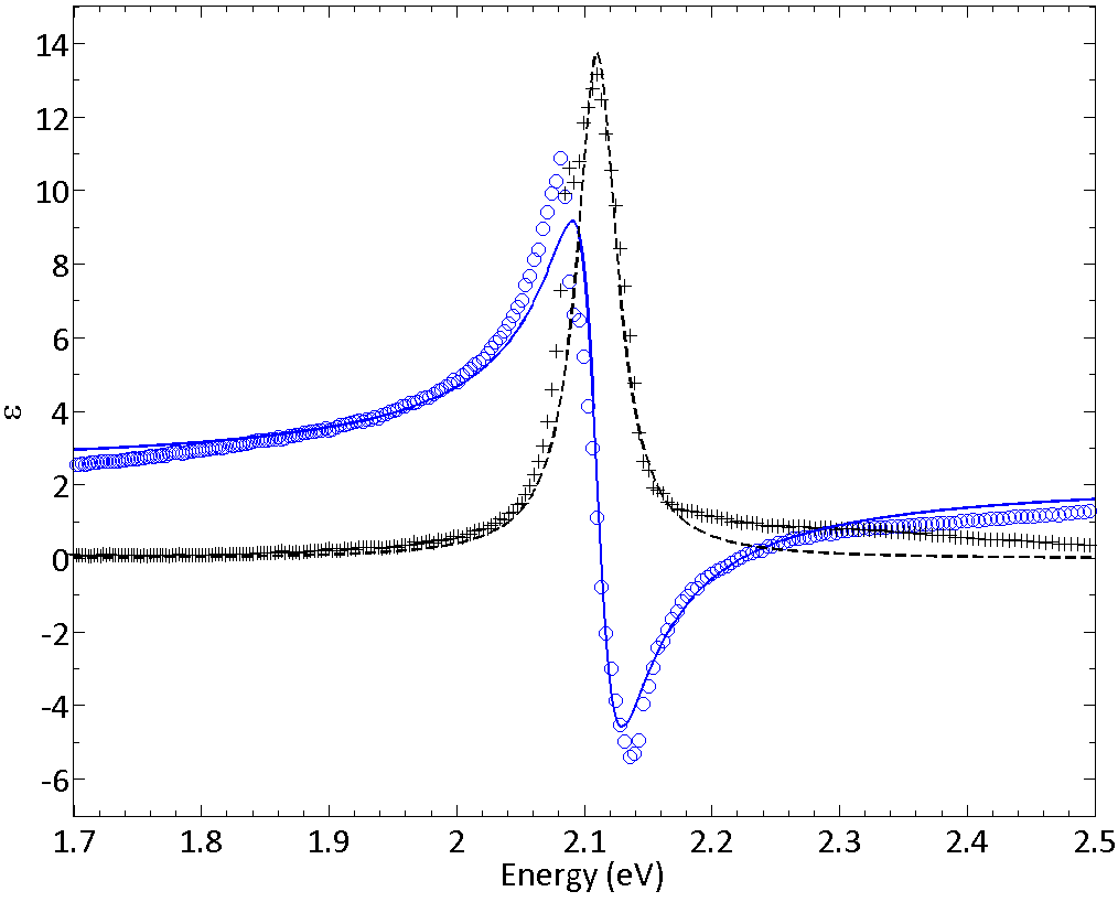
Figure 1: Extracted relative permittivity $\varepsilon(\omega)$ from a $1.46~{}wt\%$ TDBC:PVA film (circles for real part and crosses for imaginary part) [12]. The theoretical fit for $\varepsilon(\omega)$ indicated by the solid and dashed lines corresponds to a concentration of $1.46~{}wt\%$ ($3.22~{}wt\%$) for a two (three) dimensional distribution of dipoles.

The permittivity of the thin film shown in Figure 1 has been modeled assuming the dipole moments of the aggregates are randomly oriented in the plane of the film. In what follows we wish to look at the optical response of a nanoparticle. For generality, and to ensure we consider an isotropic system, we will consider the dipole moments of the aggregates to be randomly oriented in three dimensions. Making this assumption requires us to increase the number density of our molecules from $1.47\times 10^{25}~{}m^{-3}$ to $3.29\times 10^{25}~{}m^{-3}$. In this way, our nanoparticle will be comprised of a material that has the same permittivity as that shown in Figure 1. In all the calculations that follow we use this number density, which corresponds to a concentration of TDBC in PVA of $3.22~{}wt\%$.

3.1 Numerical Results: Steady-State

We now explore theoretically the Mie [20, 21] absorption efficiency spectra $Q_{abs}(\omega)$ for a $100~{}nm$ diameter nanosphere of $3.22\%$ TDBC:PVA, assuming a volume distribution of dipole orientations, based on $\varepsilon(\omega)$ calculated using Equation (14). In practice, the applied optical field we model here might be a laser beam. For a $1~{}mW$ laser with a spot diameter of $1.5~{}mm$, the strength of the electric field of our incident optical field would be equal to $462~{}Vm^{-1}$; we assume this value here.

In a $100~{}nm$ diameter nanosphere of our material, there are on average $n=1.72\times 10^{4}$ molecules. Note that it is the number of molecules and by extension their number density, which is the important quantity (and is used for $N$ in Equation (14)) rather than the number density of aggregates, since each molecule provides a potential site for exciton excitation. To check the validity of our assumption that multi-exciton and nonlinear effects [43] can be neglected, we computed the maximum expectation value of the number of excitons in the nanosphere ($n_{ex}=\max(\rho_{11})n$) using Equations (10) and (11) in Equation (12). We found that $n_{ex}/n\ll 1$ holds for laser powers of up to $10^{2}~{}W$ with a spot size of $1.5~{}mm$. Given that our laser power is $1~{}mW$, we assumed that the single-exciton linear regime is sufficient to describe the system under this illumination power.

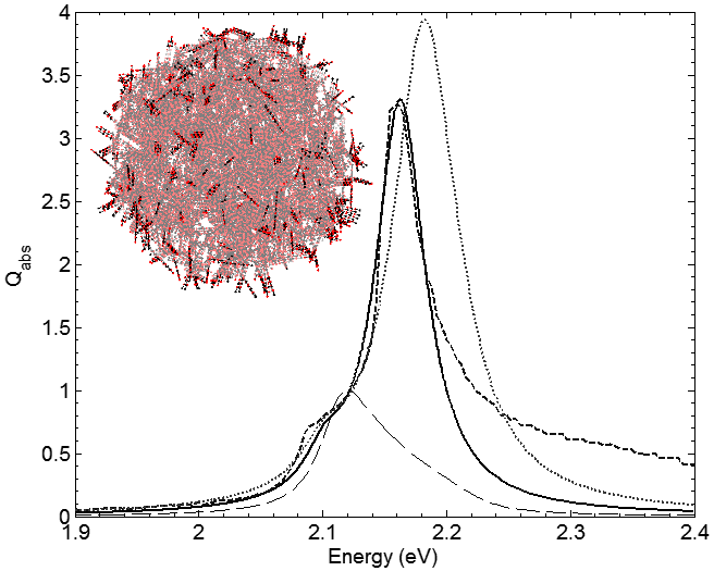
Figure 2: Mie calculations for the absorption efficiency $Q_{abs}(\omega)$ in the steady-state for a $100~{}nm$ diameter nanosphere of $3.22~{}wt\%$ TDBC:PVA using the values for $\varepsilon(\omega)$ from experiment (dashed line), from two-level OBEs (solid line), and from our previous Lorentz oscillator model (dotted line). The material absorption coefficient $\kappa$ (imaginary part of the refractive index), normalized to unity, is also plotted for illustrative purposes (long dashed line). Inset: a 3D representation of the aggregated emitters (assuming brick-stone aggregation, with 15 molecules per aggregate) randomly distributed in a $100~{}nm$ diameter nanosphere.

In Figure 2 we plot the absorption efficiency $Q_{abs}(\omega)$ for a $100~{}nm$ diameter nanosphere, calculated for a variety of permittivities; in each case the absorption efficiency is calculated using Mie theory [20, 21]. Calculated values for $Q_{abs}$ based upon the permittivity obtained using our improved analysis of experimental data are shown in Figure 2 as a dashed line. Our quantum theoretical spectrum for $Q_{abs}$, using $\varepsilon(\omega)$ from Equation (14), is shown as the solid line. This theoretically derived spectrum provides a close match to the extracted data, most importantly for energies in the region of interest below $2.22~{}eV$. For energies exceeding $2.2~{}eV$, there is a limb in the extracted data (dashed curve) which might perhaps be attributed to inhomogeneous (non-Lorentzian) broadening which is not accounted for using the OBEs. Also displayed in Figure 2 is the result for $Q_{abs}$ using a best-fit classical Lorentz oscillator model (the parameters for which can be found in our Supporting Information) shown as a dotted line. It can be seen that the quantum model outlined in the present paper provides an improved fit to the experimental data. We attribute this to the inclusion of dephasing ($\Gamma_{01}^{(d)}$) in the model: if $\Gamma_{01}^{(d)}$ were set to zero, a Lorentz model would be recovered in the steady state, and the single damping term in the Lorentz model would have to accommodate both decay and dephasing. Therefore, by including dephasing, the actual physical value of the decay rate $\gamma_{01}$ can be included to achieve an accurate result for $\varepsilon$.

It is interesting to note a key feature shown by the data in Figure 2: $Q_{abs}$, reaches its peak value at $2.16~{}eV$ ($574~{}nm$). This is in contrast to the absorption coefficient, $\kappa(\omega)$, which peaks at $2.12~{}eV$ ($586~{}nm$), shown as a long dashed line in Figure 2. This difference in spectral position arises because the peak in $Q_{abs}$ is not due simply to absorption: rather, it is due to the excitation of a localized SEP mode [12]. Confirmation of this interpretation comes from two sources. First, in the quasistatic limit the polarizability of the nanosphere follows the Clausius-Mossotti condition, for which resonance occurs when $\varepsilon$ is real-valued and equal to $-2$ (when the nanosphere is in free space) [52]. From Figure 1 this can be seen to be approximately true for our absorbing $100~{}nm$ diameter nanosphere, as the permittivity value at the wavelength of peak absorption efficiency, $Q_{abs}$, is complex and equal to $\varepsilon=-2.251+1.728i$. This difference from $\varepsilon=-2$ originates from the fact that $\varepsilon=-2$ only gives the resonance condition if the imaginary part of $\varepsilon$ is zero; the complex nature of the permittivity changes the spectral location of the absorption peak. Second, $Q_{abs}$ near the peak goes well above unity: this is associated with field enhancement [2], another signature of a resonant mode. The enhanced electric field in the vicinity of the nanosphere is illustrated graphically in Figure 3(a), together with direction of power flow shown by the Poynting vector $\bi{S}$.

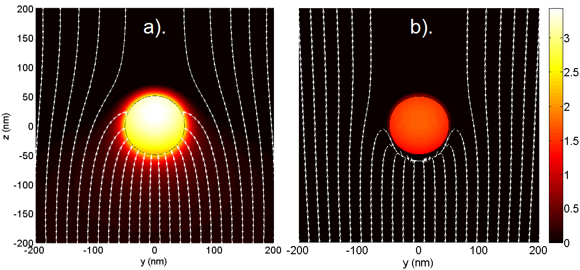
Figure 3: The time-averaged electric field strength normalized to the incident field strength (color plot) and the Poynting vector $\bi{S}$ (arrows) in the vicinity and on the surface of the $100~{}nm$ $3.22~{}wt\%$ TDBC:PVA nanosphere, with incident power flow along the positive z-direction. Data are calculated for incident photon energies of a). $2.16~{}eV=574~{}nm$ and b). $2.12~{}eV=586~{}nm$ corresponding to peak absorption efficiency and $\kappa$ respectively.

In  Figure 3, the incident electric field is polarized in the x-direction. The Poynting vector arrows shown in the figure were calculated at starting points for which $z=-200~{}nm$ and $x=0~{}nm$, linearly spaced in the range $-200~{}nm\leq y\leq 200~{}nm$. Subsequent points for evaluation of the Poynting vector were taken at $10~{}nm$ steps in the direction of the Poynting vector at each point, resulting in the flux lines shown. The power flow in Figure 3(a) shows that incident light is drawn towards and absorbed by the nanosphere for starting positions up to around $130~{}nm$ from the central position of the nanosphere. This demonstrates that at this energy, the nanosphere absorbs more light than the light geometrically striking it [53], and hence $Q_{abs}>1$. In comparison, absorption at the transition energy, i.e. at $2.11~{}eV$ is seen only as a shoulder mode in the absorption efficiency of the nanosphere (Figure 2) and the efficiency does not exceed unity. The power flow around the nanosphere for the energy at which $\kappa$ peaks ($2.12~{}eV$) is shown in Figure 3(b), and the enhancement of the field is much weaker than for excitation on resonance at $2.16~{}eV$.

3.2 Numerical Results: Time Domain

We now turn our attention to the time domain. Our theoretical model for dynamic processes in two-level quantum systems subject to a perturbing cosine electric field is similar to models considered elsewhere [54, 55, 56, 57], but here the observable of interest arises from the temporal evolution of the coherences of the density matrix, rather than the populations. The dynamics of a two-level ensemble subject to a pulse potential has been the subject of recent investigation [58], but here we investigate a rather different case: that of a cosine potential of fixed amplitude that is switched instantaneously on at some moment in time. We do this to provide an easily soluble model that illustrates the time-dependent phenomena we wish to discuss.

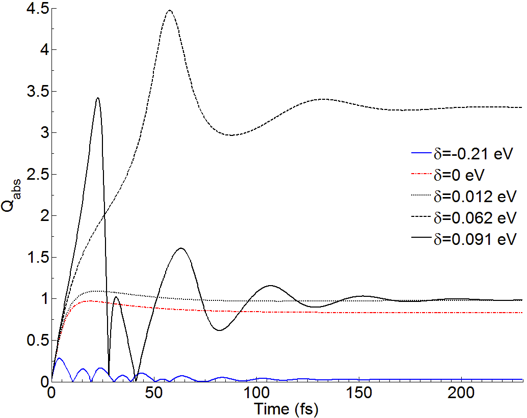
Figure 4: Calculated $Q_{abs}(t,\omega)$ for a $100~{}nm$ diameter nanosphere of $3.22\%$ TDBC:PVA warming up a pure state at $t=0$ with a $1~{}mW$ laser set at five different detunings $\delta$ from the exciton transition.

By using Equation (14) to calculate $\varepsilon(t)$ for a given illumination frequency $\omega$ as before, $Q_{abs}(t,\omega)$ can be determined and its temporal behavior examined. To do this, we again use Mie theory. This is an approximation since the fields scattered in Mie theory are assumed to be instantaneous. Given that the dynamics seen in Figure 4 evolve over a few femtoseconds and that light propagates over a length scale three times the size of the nanoparticle during a single femtosecond, and that the nanoparticle is illuminated with an electric field of constant amplitude, this approximation is deemed to hold. Mie theory can therefore be used to give a quasi-instantaneous picture of the absorption.

$Q_{abs}(t)$ is shown in Figure 4 for five different detunings, $\delta=\hbar\omega_{1}-\hbar\omega$, from the transition at $\hbar\omega_{1}=2.11~{}eV$. We assume that all the molecules in the nanoparticle are initially in their ground state. At $t=0$ we turn on our field abruptly. We see that a steady-state response is attained after $>200~{}fs$, but interestingly, for $\delta=0.09~{}eV$, $Q_{abs}(t)$ repeatedly exceeds unity in spite of the steady-state value of $Q_{abs}$ being below unity at this detuning. Since $Q_{abs}(t)>1$ implies field enhancement, these data are indicative of a transient LSEP mode being present at early times. The time-dependent behavior comprises two contributions: the first is the oscillatory behavior arising from Rabi oscillations; the second is the transient effects associated with the sudden turning-on of the field. In the latter, the magnitude of the density matrix coherences exceed their steady-state values for tens of femtoseconds, resulting in larger values of $\varepsilon$ and hence different absorption properties to the steady-state.

If $\varepsilon$ passes through the Clausius-Mossotti condition for the nanoparticle as it approaches its steady-state value, $Q_{abs}$ exceeds unity, implying a transient LSEP mode. This is seen best for a detuning of $0.091~{}eV$ between $0-30~{}fs$. The Rabi oscillations follow the generalized Rabi frequency $\tilde{\Omega}_{R}$, given by [59],

$$\tilde{\Omega}_{R}=\sqrt{\Omega_{1}^{2}+\delta^{2}},$$ (15)

where, $\Omega_{1}\ll\delta$, and $\tilde{\Omega}_{R}\rightarrow\delta$ in this case, $\Omega_{1}$ and $\delta$ are the Rabi frequency and the detuning respectively. These Rabi oscillations are naturally convoluted with the transient effects. This implies, together with the short timescales involved in the system, that it would be a challenge to see these transitory effects, but might perhaps be possible [60]. Critical to the transient LSEP lifetime is $\Gamma^{(d)}_{01}$. If this dephasing could be reduced without losing the transient negative permittivity that is essential for field enhancement (and field confinement), then the transient timescale of the system would be increased up to a maximum of $1/\gamma_{01}$. This corresponds to the picosecond regime for our TDBC:PVA system. Under this circumstance, transient LSEP modes would become more easily observable.

4 Conclusions

We have re-evaluated the measurements reported in our previous work and have obtained an improved permittivity for our J-aggregate-doped $1.46~{}wt\%$ TDBC:PVA polymer film. Using a quantum-mechanical framework we have given support to our previous investigation based on a classical analysis [12], that TDBC doped nanoparticles can exhibit a localized surface exciton-polariton (LSEP) mode. We have used a quantum model to show that these nanoparticles may also exhibit transient LSEP modes in the sub-picosecond regime. These results help strengthen the idea that molecular excitonic materials provide an interesting alternative upon which to base nanophotonics [9]. By using molecular materials the possibility of bottom-up approaches such as supramolecular chemistry and self-assembly can be brought to bear on the production of nanophotonic structures.

References

References

- [1] Le Ru E C and Etchegoin P G 2009 Principles of Surface-Enhanced Raman Spectroscopy and related plasmonic effects 1st ed (Elsevier)
- [2] Kreibig U and Vollmer M 1995 Optical Properties of Metal Clusters 1st ed (Springer-Verlag)
- [3] Kelly K L, Coronado E, Zhao L L and Schatz G C 2003 J. Phys. Chem. B 107 668–677
- [4] Stiles P L, Dieringer D J, Shah N C and Van Duyne R 2008 Ann. Rev. Anal. Chem. 1 601–626
- [5] Willets K A and Van Duyne R P 2007 Annu. Rev. Phys. Chem. 58 267–97
- [6] Taylor R W, Benz F, Sigle D O, Bowman R W, Bao P, Roth J S, Heath G R, Evans S D and Baumberg J J 2014 Scientific Reports 4 1–6
- [7] Kitson S C, Barnes W L and Sambles J R 1995 Physical Review B 52 11441–11446
- [8] Isaac T H, Barnes W L and Hendry E 2008 Applied Physics Letters 93 2008–2010
- [9] Saikin S K, Eisfeld A, Valleau S and Aspuru-Guzik A 2013 Nanophotonics 2 17 (Preprint 1304.0124)
- [10] Philpott M R, Brillante A, Pockrand I and Swalen J D 1979 Mol. Cryst. Liq. Cryst. 50 139–162
- [11] Lei Gu, Livenere J, Zhu G, Narimanov E E and Noginov M A 2013 Appl. Phys. Lett. 103 021104
- [12] Gentile M G, Nunez-Sanchez S and Barnes W L 2014 Nano Lett. 14 2339–2344
- [13] Triolo C, Cacciola A, Stefano O D, Genco A, Mazzeo M, Patanè S, Saija R and Savasta S 2015 ACS Photonics 2 971–979
- [14] Azzam R M A and Bashara N M 1977 Ellipsometry and polarized light 1st ed (North-Holland)
- [15] Lidzey D G, Bradley D D C, Armitage A, Walker S and Skolnick M S 2000 Science 288 1620–1623
- [16] Dintinger J, Klein S, Bustos F, Barnes W L and Ebbesen T W 2005 Physical Review B 71 035424
- [17] Törmä P and Barnes W L 2015 Reports on Progress in Physics 78 013901
- [18] Fox M 2010 Optical Properties of Solids 2nd ed (Oxford: Oxford University Press) ISBN 978-0-19-957336-3
- [19] Lebedev V S and Medvedev A S 2012 Quant. Electron. 42(8) 701–713
- [20] Mie G 1908 Ann. Phys. (Berlin) 25 377–445
- [21] Bohren C F and Huffman D R 1983 Absorption and Scattering of Light by Small Particles (Pennsylvania State University: Wiley)
- [22] Mandel L and Wolf E 1995 Optical Coherence and Quantum Optics (Cambridge: Cambridge University Press)
- [23] Skinner J L and Hsu D 1986 J. Phys. Chem. 90 4931–4938
- [24] Abramavicius D, Butkus V and Valkunas L 2011 Interplay of exciton coherence and dissipation in molecular aggregates Quantum Efficiency in Complex Systems, Part II: From Molecular Aggregates to Organic Solar Cells (Semiconductor and Semimetals vol 85) ed Wurfel U, Thorwart M and Weber E (London: Elsevier) chap 1, pp 3–45
- [25] Harris D C and Bertolucci M D 1989 Symmetry and Spectroscopy: an Introduction to Vibrational and Electronic Spectroscopy (New York: Dover Publications)
- [26] E D, McCumber and Sturge M D 1963 J. Appl. Phys. 34 1682
- [27] Harris C B 1977 J. Chem. Phys. 67 5607
- [28] Ambrosek D, Köhn A, Schulze J and Kühn O 2012 The Journal of Physical Chemistry A 116 11451–11458 pMID: 22946964
- [29] Miura Y F and Ikegami K 2012 J-aggregates in the langmuir and langmuir-blodgett films of merocyanine dyes J-Aggregates vol 2 ed Kobayashi T (London: World Scientific) chap 14, pp 443–514
- [30] Valleau S, Saikin S K, Yung M H and Guzik A A 2012 J. Chem. Phys. 137 034109
- [31] Spano F C 2012 Vibronic coupling in j-aggregates J-Aggregates vol 2 ed Kobayashi T (London: World Scientific) chap 2, pp 49–75
- [32] Zhao Y S 2015 Organic Nanophotonics (Berlin: Springer)
- [33] Parker S P 1993 McGraw-Hill Encyclopaedia of Physics (New York: McGraw-Hill Companies)
- [34] Knoester J 2002 Optical properties of molecular aggregates Proceedings of the International School of Physics: Enrico Fermi, Course CLIX vol 149 (IOS Press) pp 149–186
- [35] Malyshev V and Moreno P 1995 Phys. Rev. B 51 14587–14593
- [36] Hochstrasser R M and Whiteman J D 1972 J. Chem. Phys. 56 5945–5958
- [37] Houdré R, Stanley R P and Ilegems M 1996 Phys. Rev. A 53(4) 2711–2715
- [38] Kuhn H and Kuhn C 1996 Chromophore coupling effects J-Aggregates ed Kobayashi T (London: World Scientific) chap 1, pp 1–40
- [39] Blum K 1996 Density matrix theory and application 2nd ed (New York: Plenum Press)
- [40] Schirmer S G and Solomon A I 2004 Phys. Rev. A 70 022107
- [41] Breuer H P and Petruccione F 2002 The Theory of Open Quantum Systems (New York: Oxford University Press)
- [42] Schaller G and Brandes T 2008 Phys. Rev. A 78(2) 022106
- [43] Wang K and Chu S I 1987 J. Chem. Phys. 86(6) 3225–3238
- [44] del Pino J, Feist J and Garcia-Vidal F J 2015 New Journal of Physics 17 053040 URL http://stacks.iop.org/1367-2630/17/i=5/a=053040
- [45] Kavanaugh T C and Silbey R J 1993 J. Chem. Phys. 98(12) 9444–9454
- [46] Allen L and Eberly J H 1975 Optical Resonance and Two-Level Atoms (New York: Wiley)
- [47] Dorfman K E, Jha P K, Voronine D V, Genevet P, Capasso F and Scully M O 2013 Phys. Rev. Lett. 111 043601
- [48] van Burgel M, Wiersma D A and Duppen K 1995 The Journal of Chemical Physics 102 20–33
- [49] Wang S, Chervy T, George J, Hutchison J A and Genet C 2014 J. Phys. Chem. Lett. 5 1433–1439
- [50] Garrett S H, Wasey J A E and Barnes W L 2004 Journal of Modern Optics 51 2287–2295
- [51] Bradley M S, Tischler J R and Bulović V 2005 Adv. Mater. 17 1881–1886
- [52] Novotny L and Hecht B 2006 Principles of Nano-Optics 1st ed (Cambridge University Press)
- [53] Bohren C F 1983 Am. J. Phys. 51 323–327
- [54] Fox M 2010 Quantum Optics An Introduction (University of Sheffield: Oxford University Press)
- [55] Foot C J 2011 Atomic Physics (Oxford: Oxford University Press)
- [56] Slowik K, Filter R, Straubel J, , Lederer F and Rockstuhl C 2013 Phys. Rev. B 88 195414
- [57] Noh H R and Jhe W 2010 Opt Commun 283 2353–2355
- [58] Sukharev M, Seideman T, Gordon R J, Salomon A and Prior Y 2014 ACS Nano 8(1) 807–817
- [59] Harter D J, Narum P, Raymer M G and Boyd R W 1981 Phys. Rev. Lett. 46(18) 1192–1195
- [60] Vasa P, Wang W, Pomraenke R, Lammers M, Maiuri M, Manzoni C, Cerullo G and Lienau C 2013 Nature Photonics 7 128–132