Priority Choice Experimental Two-qubit Tomography:
Karol Bartkiewicz
bark@amu.edu.pl
Faculty of Physics, Adam
Mickiewicz University, PL-61-614 Poznań, Poland
RCPTM, Joint Laboratory of Optics of Palacký
University and Institute of Physics of Academy of Sciences of the
Czech Republic, 17. listopadu 12, 772 07 Olomouc, Czech Republic
Antonín Černoch
RCPTM, Joint Laboratory of Optics of Palacký
University and Institute of Physics of Academy of Sciences of the
Czech Republic, 17. listopadu 12, 772 07 Olomouc, Czech Republic
Institute of Physics of Academy of Science of the
Czech Republic, Joint Laboratory of Optics of Palacký University
and Institute of Physics of Academy of Sciences of the Czech
Republic, 17. listopadu 50A, 77207 Olomouc, Czech Republic
Karel Lemr
RCPTM, Joint Laboratory of Optics of Palacký
University and Institute of Physics of Academy of Sciences of the
Czech Republic, 17. listopadu 12, 772 07 Olomouc, Czech Republic
Adam Miranowicz
CEMS, RIKEN, 351-0198 Wako-shi, Japan
Faculty of Physics, Adam Mickiewicz University,
PL-61-614 Poznań, Poland
Abstract
In standard optical tomographic methods, the off-diagonal
elements of a density matrix ρ 𝜌 \rho ρ 𝜌 \rho 90 ,
062123 (2014)] has been proposed theoretically to measure
one-by-one all the elements of ρ 𝜌 \rho
pacs: 03.65.Wj, 03.67.-a, 42.50.Ex
Introduction.— Quantum tomographic methods are
indispensable tools in experimental quantum physics. Indeed,
characterizing quantum states and quantum processes are
essential problems in studying the performance and evolution of
quantum systems ParisBook Georgescu12 NielsenBook James01 ; Rehacek01 ; Blume10a ; Teo11 ; Teo12 ; Smolin12 ; Halenkova2012 ; Halenkova2012a ; Bart12 ; Bart13a ; Bart14 Opatrny97 ParisBook ; Blume10b ; Huszar12 Qi13 Altepeter05review Burgh08 ; Bogdanov10a ; Adamson10 ; Sansoni10 ; Altepeter11 ; Pryde05 ; Lundeen11 ; Lundeen12 ; Salvail13 Miranowicz14 κ 𝜅 \kappa Bogdanov10a ; Bogdanov10b ; Bogdanov11a James01 Altepeter05 ; Burgh08 Adamson10
All the approaches analyzed here are based on solving a
linear-system problem A x = b 𝐴 𝑥 𝑏 Ax=b A 𝐴 A coefficient matrix , b 𝑏 {b} observation vector
containing the measured data, and x = vec ( ρ ) 𝑥 vec 𝜌 x={\rm vec}(\rho) ρ 𝜌 \rho
x = vec ( ρ ) = [ ρ 11 , Re ρ 12 , Im ρ 12 , Re ρ 13 , Im ρ 13 , … , ρ 44 ] T . 𝑥 vec 𝜌 superscript subscript 𝜌 11 Re subscript 𝜌 12 Im subscript 𝜌 12 Re subscript 𝜌 13 Im subscript 𝜌 13 … subscript 𝜌 44
𝑇 x={\rm vec}(\rho)=[\rho_{11},{\rm Re}\rho_{12},{\rm Im}\rho_{12},{\rm Re}\rho_{13},{\rm Im}\rho_{13},...,\rho_{44}]^{T}.
Conversely, a two-qubit density matrix ρ 𝜌 \rho x = ( x 1 , … , x 16 ) 𝑥 subscript 𝑥 1 … subscript 𝑥 16 x=(x_{1},...,x_{16})
ρ ( x ) = [ x 1 x 2 + i x 3 x 4 + i x 5 x 6 + i x 7 x 2 − i x 3 x 8 x 9 + i x 10 x 11 + i x 12 x 4 − i x 5 x 9 − i x 10 x 13 x 14 + i x 15 x 6 − i x 7 x 11 − i x 12 x 14 − i x 15 x 16 ] 𝜌 𝑥 delimited-[] subscript 𝑥 1 subscript 𝑥 2 𝑖 subscript 𝑥 3 subscript 𝑥 4 𝑖 subscript 𝑥 5 subscript 𝑥 6 𝑖 subscript 𝑥 7 subscript 𝑥 2 𝑖 subscript 𝑥 3 subscript 𝑥 8 subscript 𝑥 9 𝑖 subscript 𝑥 10 subscript 𝑥 11 𝑖 subscript 𝑥 12 subscript 𝑥 4 𝑖 subscript 𝑥 5 subscript 𝑥 9 𝑖 subscript 𝑥 10 subscript 𝑥 13 subscript 𝑥 14 𝑖 subscript 𝑥 15 subscript 𝑥 6 𝑖 subscript 𝑥 7 subscript 𝑥 11 𝑖 subscript 𝑥 12 subscript 𝑥 14 𝑖 subscript 𝑥 15 subscript 𝑥 16 \rho(x)=\left[\begin{array}[]{cccc}x_{1}&x_{2}+ix_{3}&x_{4}+ix_{5}&x_{6}+ix_{7}\\
x_{2}-ix_{3}&x_{8}&x_{9}+ix_{10}&x_{11}+ix_{12}\\
x_{4}-ix_{5}&x_{9}-ix_{10}&x_{13}&x_{14}+ix_{15}\\
x_{6}-ix_{7}&x_{11}-ix_{12}&x_{14}-ix_{15}&x_{16}\\
\end{array}\right]
The already mentioned condition number κ 𝜅 \kappa A 𝐴 A b 𝑏 b ρ 𝜌 \rho x = A − 1 b 𝑥 superscript 𝐴 1 𝑏 x=A^{-1}b A 𝐴 A b 𝑏 b κ 𝜅 \kappa AtkinsonBook A x = b 𝐴 𝑥 𝑏 Ax=b A 𝐴 A δ b 𝛿 𝑏 \delta b b 𝑏 b δ x 𝛿 𝑥 \delta x A ( x + δ x ) = b + δ b , 𝐴 𝑥 𝛿 𝑥 𝑏 𝛿 𝑏 A(x+\delta\,x)=b+\delta\,b, AtkinsonBook
1 κ ( A ) ‖ δ b ‖ ‖ b ‖ ≤ ‖ δ x ‖ ‖ x ‖ ≤ κ ( A ) ‖ δ b ‖ ‖ b ‖ . 1 𝜅 𝐴 norm 𝛿 𝑏 norm 𝑏 norm 𝛿 𝑥 norm 𝑥 𝜅 𝐴 norm 𝛿 𝑏 norm 𝑏 \frac{1}{\kappa(A)}\frac{||\delta b||}{||b||}\leq\frac{||\delta x||}{||x||}\leq\kappa(A)\frac{||\delta b||}{||b||}. (1)
Thus, if the condition number κ ( A ) 𝜅 𝐴 \kappa(A) b 𝑏 b x 𝑥 x κ ( A ) ≡ cond 2 ( A ) = σ max ( A ) / σ min ( A ) 𝜅 𝐴 subscript cond 2 𝐴 subscript 𝜎 𝐴 subscript 𝜎 𝐴 \kappa(A)\equiv{\rm cond}_{2}(A)=\sigma_{\max}(A)/{\sigma_{\min}(A)} ‖ A ‖ 2 subscript norm 𝐴 2 \|A\|_{2} ∥ ⋅ ∥ \|\cdot\| 1 A 𝐴 A ‖ A ‖ 2 = max [ svd ( A ) ] ≡ σ max ( A ) , subscript norm 𝐴 2 svd 𝐴 subscript 𝜎 𝐴 \|A\|_{2}=\max[{\rm svd}(A)]\equiv\sigma_{\max}(A), svd ( A ) svd 𝐴 {\rm svd}(A) A 𝐴 A Miranowicz14 κ ( A ) = 1 𝜅 𝐴 1 \kappa(A)=1 James01 κ ( A ) = 60.1 𝜅 𝐴 60.1 \kappa(A)=\sqrt{60.1} Altepeter05 ; Burgh08 κ ( A ) = 3 𝜅 𝐴 3 \kappa(A)=3 Adamson10 ; Bandyopadhyay01 κ ( A ) = 5 𝜅 𝐴 5 \kappa(A)=\sqrt{5} κ ( A ) = 2 𝜅 𝐴 2 \kappa(A)=\sqrt{2} κ 𝜅 \kappa
Error analysis.— From the linearity of the linear
inversion problem and Eq. (1
1 κ ( A ) ‖ δ b ‖ ‖ b + δ b ‖ ≤ ‖ δ x ‖ ‖ x + δ x ‖ ≤ κ ( A ) ‖ δ b ‖ ‖ b + δ b ‖ . 1 𝜅 𝐴 norm 𝛿 𝑏 norm 𝑏 𝛿 𝑏 norm 𝛿 𝑥 norm 𝑥 𝛿 𝑥 𝜅 𝐴 norm 𝛿 𝑏 norm 𝑏 𝛿 𝑏 \frac{1}{\kappa(A)}\frac{\|\delta b\|}{||b+\delta b||}\leq\frac{\|\delta x\|}{\|x+\delta x\|}\leq\kappa(A)\frac{\|\delta b\|}{\|b+\delta b\|}. (2)
Let us quantify the quality of a tomography protocol with the
trace distance E ≡ T [ ρ ( x ) , ρ ( x + δ x ) ] = 1 2 Tr ( δ ρ ) 2 𝐸 𝑇 𝜌 𝑥 𝜌 𝑥 𝛿 𝑥 1 2 Tr superscript 𝛿 𝜌 2 E\equiv T[\rho(x),\rho(x+\delta x)]=\tfrac{1}{2}{\rm Tr}\sqrt{(\delta\rho)^{2}} δ ρ ≡ ρ ( δ x ) 𝛿 𝜌 𝜌 𝛿 𝑥 \delta\rho\equiv\rho(\delta x) ρ ( x ) 𝜌 𝑥 \rho(x) ρ ( x + δ x ) 𝜌 𝑥 𝛿 𝑥 \rho(x+\delta x) E 𝐸 E ‖ δ x ‖ norm 𝛿 𝑥 \|\delta x\| ( δ ρ ) 2 superscript 𝛿 𝜌 2 \sqrt{(\delta\rho)^{2}}
2 E = Tr ( δ ρ ) 2 ≤ d Tr [ ( δ ρ ) 2 ] ≤ 2 d ‖ δ x ‖ , 2 𝐸 Tr superscript 𝛿 𝜌 2 𝑑 Tr delimited-[] superscript 𝛿 𝜌 2 2 𝑑 norm 𝛿 𝑥 2E={\rm Tr}\sqrt{(\delta\rho)^{2}}\leq\sqrt{d\,{\rm Tr}[(\delta\rho)^{2}]}\leq\sqrt{2d}\,\|\delta x\|, (3)
where, for a two-qubit density matrix, Tr [ ( δ ρ ) 2 ] = 2 ∑ i = 1 16 δ x i 2 − ( δ x 1 2 + δ x 5 2 + δ x 13 2 + δ x 16 2 ) Tr delimited-[] superscript 𝛿 𝜌 2 2 subscript superscript 16 𝑖 1 𝛿 subscript superscript 𝑥 2 𝑖 𝛿 subscript superscript 𝑥 2 1 𝛿 subscript superscript 𝑥 2 5 𝛿 subscript superscript 𝑥 2 13 𝛿 subscript superscript 𝑥 2 16 {\rm Tr}[(\delta\,\rho)^{2}]=2\sum^{16}_{i=1}\delta x^{2}_{i}-(\delta x^{2}_{1}+\delta x^{2}_{5}+\delta x^{2}_{13}+\delta x^{2}_{16}) d = 4 𝑑 4 d=4 2 3
E ≤ d 2 κ ( A ) ‖ δ b ‖ ‖ x + δ x ‖ ‖ b + δ b ‖ , 𝐸 𝑑 2 𝜅 𝐴 norm 𝛿 𝑏 norm 𝑥 𝛿 𝑥 norm 𝑏 𝛿 𝑏 E\leq\sqrt{\frac{d}{2}}\,\kappa(A)\,\frac{\|\delta b\|\|x+\delta x\|}{\|b+\delta b\|}, (4)
where the random deviations δ b 𝛿 𝑏 \delta b σ ( b ) 𝜎 𝑏 \sigma(b) b 𝑏 b b + δ b 𝑏 𝛿 𝑏 b+\delta b b + δ b 𝑏 𝛿 𝑏 b+\delta\,b b + δ b ≈ b = σ 2 ( b ) 𝑏 𝛿 𝑏 𝑏 superscript 𝜎 2 𝑏 b+\delta\,b\approx b=\sigma^{2}(b) δ b 𝛿 𝑏 \delta b | δ b i | > 2 2 b i 𝛿 subscript 𝑏 𝑖 2 2 subscript 𝑏 𝑖 |\delta\,b_{i}|>2\sqrt{2b_{i}} CDF CDF \mathrm{CDF} Pr ( | δ b i | > 2 2 b i ) = CDF ( x + ) − CDF ( x − ) Pr 𝛿 subscript 𝑏 𝑖 2 2 subscript 𝑏 𝑖 CDF subscript 𝑥 CDF subscript 𝑥 \mathrm{Pr}(|\delta\,b_{i}|>2\sqrt{2b_{i}})=\mathrm{CDF}(x_{+})-\mathrm{CDF}(x_{-}) x ± = ⌊ b i ± 2 2 b i ⌋ subscript 𝑥 plus-or-minus plus-or-minus subscript 𝑏 𝑖 2 2 subscript 𝑏 𝑖 x_{\pm}=\lfloor b_{i}\pm 2\sqrt{2b_{i}}\rfloor CDF ( x < 0 ) = 0 CDF 𝑥 0 0 \mathrm{CDF}(x<0)=0 Pr ( | δ b i | > 2 2 b i ) > 0.981 Pr 𝛿 subscript 𝑏 𝑖 2 2 subscript 𝑏 𝑖 0.981 \mathrm{Pr}(|\delta\,b_{i}|>2\sqrt{2b_{i}})>0.981 b i subscript 𝑏 𝑖 b_{i} b i > 20 subscript 𝑏 𝑖 20 b_{i}>20 Pr ( | δ b i | > 2 2 b i ) > 0.993 Pr 𝛿 subscript 𝑏 𝑖 2 2 subscript 𝑏 𝑖 0.993 \mathrm{Pr}(|\delta\,b_{i}|>2\sqrt{2b_{i}})>0.993 3 σ 3 𝜎 3\sigma 0.997 0.997 0.997 | δ b i | < 3 σ ( b i ) 𝛿 subscript 𝑏 𝑖 3 𝜎 subscript 𝑏 𝑖 |\delta b_{i}|<3\sigma(b_{i}) | δ b i | < 2 2 σ ( b i ) 𝛿 subscript 𝑏 𝑖 2 2 𝜎 subscript 𝑏 𝑖 |\delta b_{i}|<2\sqrt{2}\sigma(b_{i})
E ≤ R ≡ 2 d κ ( A ) ‖ σ ( b ) ‖ ‖ x + δ x ‖ ‖ b + δ b ‖ . 𝐸 𝑅 2 𝑑 𝜅 𝐴 norm 𝜎 𝑏 norm 𝑥 𝛿 𝑥 norm 𝑏 𝛿 𝑏 E\leq R\equiv 2\sqrt{d}\,\kappa(A)\,\frac{\|\sigma(b)\|\|x+\delta x\|}{\|b+\delta b\|}. (5)
We have defined the uncertainty radius of the state estimation
R 𝑅 R ρ 𝜌 \rho R 𝑅 R R 𝑅 R
However, using the uncertainty radius R 𝑅 R E 𝐸 E k = ‖ δ b ‖ / ‖ σ ( b ) ‖ 𝑘 norm 𝛿 𝑏 norm 𝜎 𝑏 k=\|\delta b\|/\|\sigma(b)\| 0 ≤ k ≤ 2 2 0 𝑘 2 2 0\leq k\leq 2\sqrt{2}
k R 4 d κ 2 ( A ) ≤ E ≤ k R 2 2 , 𝑘 𝑅 4 𝑑 superscript 𝜅 2 𝐴 𝐸 𝑘 𝑅 2 2 \frac{kR}{4\sqrt{d}\kappa^{2}(A)}\leq E\leq\frac{kR}{2\sqrt{2}}, (6)
where the lower bound is derived with help of Eqs. (4 5 D HS ( ρ , ρ + δ ρ ) = Tr [ ( δ ρ ) 2 ] ≤ 2 E subscript 𝐷 HS 𝜌 𝜌 𝛿 𝜌 Tr delimited-[] superscript 𝛿 𝜌 2 2 𝐸 D_{\mathrm{HS}}(\rho,\rho+\delta\,\rho)=\sqrt{{\rm Tr}[(\delta\,\rho)^{2}]}\leq 2E b i subscript 𝑏 𝑖 b_{i} k R / 2 2 𝑘 𝑅 2 2 {kR}/{2\sqrt{2}} 1 − 1 / k 2 1 1 superscript 𝑘 2 1-1/k^{2} 50 % percent 50 50\% 2 2 \sqrt{2} R / 2 𝑅 2 R/2 E 𝐸 E b i + δ b i > b i + k σ ( b i ) subscript 𝑏 𝑖 𝛿 subscript 𝑏 𝑖 subscript 𝑏 𝑖 𝑘 𝜎 subscript 𝑏 𝑖 b_{i}+\delta\,b_{i}>b_{i}+k\sigma(b_{i}) Pr ( X > x ) ≤ e − μ ( e μ / x ) x Pr 𝑋 𝑥 superscript e 𝜇 superscript e 𝜇 𝑥 𝑥 \mathrm{Pr}(X>x)\leq\mathrm{e}^{-\mu}(\mathrm{e}\mu/x)^{x} Mitzenmacher X = b i + δ b i 𝑋 subscript 𝑏 𝑖 𝛿 subscript 𝑏 𝑖 X=b_{i}+\delta\,b_{i} μ = b i 𝜇 subscript 𝑏 𝑖 \mu=b_{i} x = μ + k μ 𝑥 𝜇 𝑘 𝜇 x=\mu+k\sqrt{\mu}
For characterizing the quality of tomographic protocols we can
also introduce the disturbance D B ( ρ , ρ + δ ρ ) = 1 − [ Tr ρ ( ρ + δ ρ ) ρ ] 2 = 1 − F ( ρ , ρ + δ ρ ) subscript 𝐷 𝐵 𝜌 𝜌 𝛿 𝜌 1 superscript delimited-[] Tr 𝜌 𝜌 𝛿 𝜌 𝜌 2 1 𝐹 𝜌 𝜌 𝛿 𝜌 D_{B}(\rho,\rho+\delta\rho)=1-[{\rm Tr}\sqrt{\sqrt{\rho}(\rho+\delta\rho)\sqrt{\rho}}]^{2}=1-F(\rho,\rho+\delta\,\rho) F 𝐹 F D B ( ρ , ρ + δ ρ ) ≤ T ( ρ , ρ + δ ρ ) subscript 𝐷 𝐵 𝜌 𝜌 𝛿 𝜌 𝑇 𝜌 𝜌 𝛿 𝜌 D_{B}(\rho,\rho+\delta\rho)\leq T(\rho,\rho+\delta\rho) D B ≤ E ≤ R subscript 𝐷 𝐵 𝐸 𝑅 D_{B}\leq E\leq R Adamson10
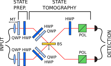
Figure 1: Experimental setup performing both
local and nonlocal polarization projections for the four studied
tomographies. Linear-optical components are quarter-wave plate
(QWP), half-wave plate (QWP), motorized translation (MT) to
stabilize two-photon overlap, horizontally retractable balanced
beam splitter (BS), polarizing cube (POL).
Experimental results.— The results obtained in the
previous section suggest that the error E 𝐸 E κ ( A ) 𝜅 𝐴 \kappa(A) b i subscript 𝑏 𝑖 b_{i} { H H , H V , V H , V V } 𝐻 𝐻 𝐻 𝑉 𝑉 𝐻 𝑉 𝑉 \{HH,HV,VH,VV\} ρ 11 = x 1 subscript 𝜌 11 subscript 𝑥 1 \rho_{11}=x_{1} | H H ⟩ ket 𝐻 𝐻 |HH\rangle et al. source
Kwiat99 2.10 3 superscript 2.10 3 2.10^{3} 1
In order to perform local projections on individual photons, we
have shifted the beam splitter BS horizontally so that the
reflections are no longer coupled to the output ports. Then for
each local projection, we have adjusted the HWP and QWP in each
photon’s path and then subjected the photons to a polarizing cube.
Respective two-photon detections were registered for 5 seconds.
The nonlocal projections are achieved by combining the local state
transformations using the HWPs and QWPs with the singlet-state
projection on a balanced beam splitter BS. For this procedure to
work, an additional HWP (set to 45 ∘ superscript 45 45^{\circ}
While evidently the beam splitter is superfluous for local
projections and the polarizing cubes are unnecessary for the
nonlocal projections, we maintain all the components in the setup
for all times deliberately since we need to compare the observed
detection rates across local and nonlocal measurements. This would
be problematic without keeping all the components in the setup
since the components introduce different technological losses
(e.g. back-reflections, scattering). Further to that, our setup
allows to switch between the local and nonlocal projections
without much effort.
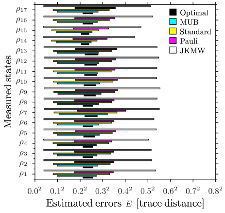
Figure 2: Experimentally recovered range of possible
errors E 𝐸 E E , 𝐸 E, 6 k = 2 𝑘 2 k=\sqrt{2} R 𝑅 R r = R / 2 𝑟 𝑅 2 r=R/2 5
For each tomography we have gathered the coincidence counts
b + δ b 𝑏 𝛿 𝑏 b+\delta b supplement b + δ b ≈ b = σ 2 ( b ) 𝑏 𝛿 𝑏 𝑏 superscript 𝜎 2 𝑏 b+\delta\,b\approx b=\sigma^{2}(b) b i subscript 𝑏 𝑖 b_{i} σ ( b i ) 𝜎 subscript 𝑏 𝑖 \sigma(b_{i}) b i + δ b i subscript 𝑏 𝑖 𝛿 subscript 𝑏 𝑖 b_{i}+\delta\,b_{i} < ( 2 2 / b i ) 1 / 2 absent superscript 2 2 subscript 𝑏 𝑖 1 2 <{(2\sqrt{2}/\sqrt{b_{i}})^{1/2}} b i ≈ 10 3 subscript 𝑏 𝑖 superscript 10 3 b_{i}\approx 10^{3} σ ( b i ) 𝜎 subscript 𝑏 𝑖 \sigma(b_{i}) ‖ σ ( b ) ‖ norm 𝜎 𝑏 \|\sigma(b)\| ‖ σ ( b ) ‖ norm 𝜎 𝑏 \|\sigma(b)\| 1.3 1.3 1.3 b + δ b 𝑏 𝛿 𝑏 b+\delta b Miranowicz14 c i subscript 𝑐 𝑖 c_{i} c i ′ subscript superscript 𝑐 ′ 𝑖 c^{\prime}_{i} b 𝑏 b b i = ⌊ ( c i − c i ′ ) / 2 ⌋ subscript 𝑏 𝑖 subscript 𝑐 𝑖 subscript superscript 𝑐 ′ 𝑖 2 b_{i}=\lfloor(c_{i}-c^{\prime}_{i})/2\rfloor σ 2 ( b i ) = ⌊ ( c i + c i ′ ) / 2 ⌋ superscript 𝜎 2 subscript 𝑏 𝑖 subscript 𝑐 𝑖 subscript superscript 𝑐 ′ 𝑖 2 \sigma^{2}(b_{i})=\lfloor(c_{i}+c^{\prime}_{i})/2\rfloor > 0.993 absent 0.993 >0.993 c i , c i ′ > 20 subscript 𝑐 𝑖 subscript superscript 𝑐 ′ 𝑖
20 c_{i},\,c^{\prime}_{i}>20 δ b i ≤ ⌊ 2 2 σ ( b i ) ⌋ 𝛿 subscript 𝑏 𝑖 2 2 𝜎 subscript 𝑏 𝑖 \delta\,b_{i}\leq\lfloor 2\sqrt{2}\sigma(b_{i})\rfloor 2 E 𝐸 E κ 𝜅 \kappa r = R / 2 𝑟 𝑅 2 r=R/2 3 supplement
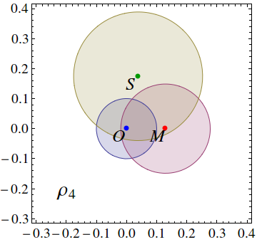
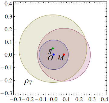
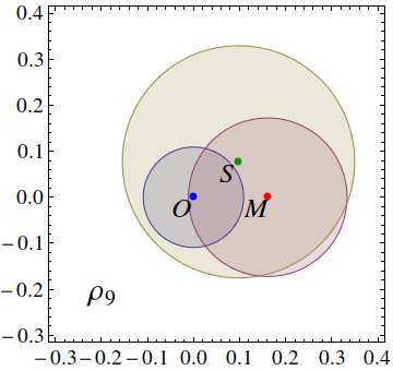
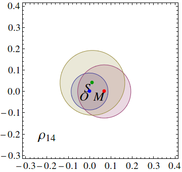
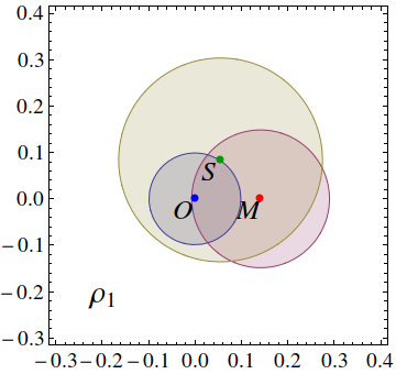
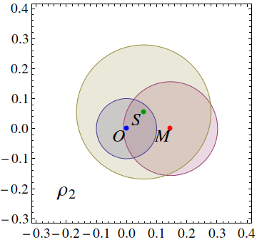
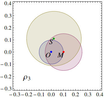
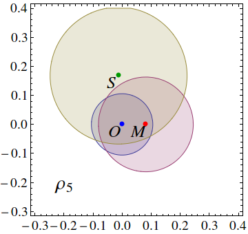
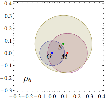
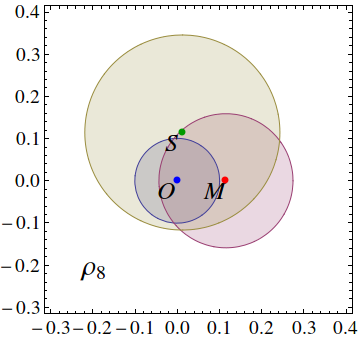
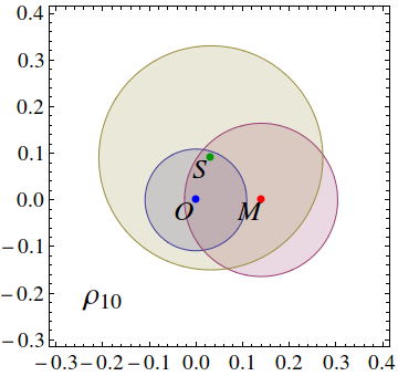
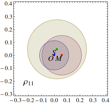
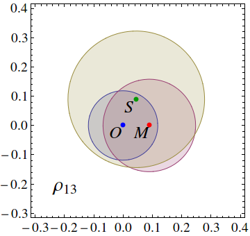
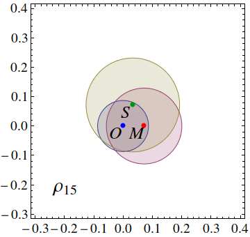
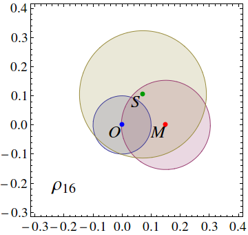
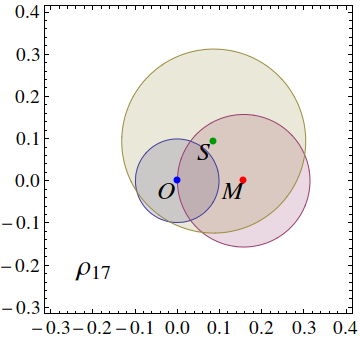
Figure 3: Relative trace distances between points
corresponding to optimal tomography (O 𝑂 O S 𝑆 S M 𝑀 M R 𝑅 R ρ n = | ψ n ⟩ ⟨ ψ n | subscript 𝜌 𝑛 | ψ n ⟩ ⟨ ψ n | \rho_{n}=\mbox{$|\psi_{n}\rangle$}\mbox{$\langle\psi_{n}|$} | ψ 4 ⟩ = ( | D R ⟩ − i | A L ⟩ ) / 2 ket subscript 𝜓 4 ket 𝐷 𝑅 𝑖 ket 𝐴 𝐿 2 \mbox{$|\psi_{4}\rangle$}=(\mbox{$|DR\rangle$}-i\mbox{$|AL\rangle$})/\sqrt{2} | ψ 7 ⟩ = | H V ⟩ ket subscript 𝜓 7 ket 𝐻 𝑉 \mbox{$|\psi_{7}\rangle$}=\mbox{$|HV\rangle$} | ψ 9 ⟩ = ( | H V ⟩ − | V H ⟩ ) / 2 ket subscript 𝜓 9 ket 𝐻 𝑉 ket 𝑉 𝐻 2 \mbox{$|\psi_{9}\rangle$}=(\mbox{$|HV\rangle$}-\mbox{$|VH\rangle$})/\sqrt{2} | ψ 14 ⟩ = | e 1 a e 1 b ⟩ ket subscript 𝜓 14 ket subscript 𝑒 1 𝑎 subscript 𝑒 1 𝑏 \mbox{$|\psi_{14}\rangle$}=\mbox{$|e_{1a}e_{1b}\rangle$} | e 1 a ⟩ = ( − 0.6556 + 0.6248 i ) | H ⟩ + 0.4241 | V ⟩ ket subscript 𝑒 1 𝑎 0.6556 0.6248 𝑖 ket 𝐻 0.4241 ket 𝑉 \mbox{$|e_{1a}\rangle$}=(-0.6556+0.6248i)\mbox{$|H\rangle$}+0.4241\mbox{$|V\rangle$} | e 1 b ⟩ = ( − 0.1415 − 0.7165 i ) | H ⟩ + 0.6831 | V ⟩ ket subscript 𝑒 1 𝑏 0.1415 0.7165 𝑖 ket 𝐻 0.6831 ket 𝑉 \mbox{$|e_{1b}\rangle$}=(-0.1415-0.7165i)\mbox{$|H\rangle$}+0.6831\mbox{$|V\rangle$} | H ⟩ ket 𝐻 |H\rangle | V ⟩ ket 𝑉 |V\rangle | D ⟩ ket 𝐷 |D\rangle | A ⟩ ket 𝐴 |A\rangle | R ⟩ ket 𝑅 |R\rangle | L ⟩ ket 𝐿 |L\rangle R 𝑅 R R / 2 , 𝑅 2 R/2, E 𝐸 E 2
Conclusions.— We have for the first time implemented
the optimal two-qubit tomography and compared it with the other
four important tomographic protocols. This method corresponds
to measuring one by one all the elements ρ n m subscript 𝜌 𝑛 𝑚 \rho_{nm} ρ 𝜌 \rho ρ 𝜌 \rho ρ n m subscript 𝜌 𝑛 𝑚 \rho_{nm}
Acknowledgements.
Acknowledgments.— K.B. acknowledges the support by the
Polish National Science Centre (Grant No. DEC-2013/11/D/ST2/02638)
and by the Foundation for Polish Science (START Programme). K.B.
and A.Č. are supported by the project No. LO1305 of the
Ministry of Education, Youth and Sports of the Czech Republic.
K.L. acknowledges support by the Czech Science Foundation (Grant
No.13-31000P). A.M. is supported by the Polish National Science
Centre under grants DEC-2011/03/B/ST2/01903 and
DEC-2011/02/A/ST2/00305.
References
(1)
M. G. A. Paris and J. Řeháček (eds.), Quantum
State Estimation , Lecture Notes in Physics, Vol. 649 (Springer,
Berlin, 2004).
(2)
I. Georgescu and F. Nori, “Quantum technologies: an old
new story,” Phys. World, p. 16 (May 2012).
(3)
M. A. Nielsen and I. L. Chuang, Quantum Computation and
Quantum Information (Cambridge University Press, Cambridge,
England, 2001).
(4)
D. F. V. James, P. G. Kwiat, W. J. Munro, and A. G. White,
“Measurement of qubits,” Phys. Rev. A 64 , 052312 (2001).
(5)
J. Řeháček, Z. Hradil, and M. Ježek,
“Iterative algorithm for reconstruction of entangled
states,” Phys. Rev. A 63 , 040303(R) (2001).
(6)
R. Blume-Kohout, “Hedged maximum likelihood quantum state
estimation,” Phys. Rev. Lett. 105 , 200504 (2010).
(7)
Y. S. Teo, H. Zhu, B. G. Englert, J. Řeháček, and Z.
Hradil, “Quantum-state reconstruction by maximizing
likelihood and entropy,” Phys. Rev. Lett. 107 , 020404 (2011).
(8)
Y. S. Teo, B. Stoklasa, B. G. Englert, J. Řeháček, and
Z. Hradil, “Incomplete quantum state estimation: A
comprehensive study,” Phys. Rev. A 85 , 042317 (2012).
(9)
J. A. Smolin, J. M. Gambetta, and G. Smith, “Efficient
method for computing the maximum-likelihood quantum state from
measurements with additive Gaussian noise,” Phys. Rev. Lett. 108 ,
070502 (2012).
(10)
E. Halenková, K. Lemr, A. Černoch, and J. Soubusta,
“Experimental simulation of a
polarization-dispersion-fluctuating channel with photon pairs,”
Phys. Rev. A 85 , 063807 (2012).
(11)
E. Halenková, A. Černoch, K. Lemr, J. Soubusta, and S.
Drusová, “Experimental implementation of the
multifunctional compact two-photon state analyzer,” Appl. Opt.
51 , 474 (2012).
(12)
K. Lemr, K. Bartkiewicz, A. Černoch, J. Soubusta, and A.
Miranowicz, “Experimental linear-optical implementation of a
multifunctional optimal cloner,” Phys. Rev. A85 , 050307(R)
(2012).
(13)
K. Bartkiewicz, K. Lemr, A. Černoch, J. Soubusta, and A.
Miranowicz, “Experimental eavesdropping based on optimal
quantum cloning,” Phys. Rev. Lett. 110 , 173601 (2013).
(14)
K. Bartkiewicz, A. Černoch, K. Lemr, J. Soubusta, and M.
Stobińska, “Efficient amplification of photonic qubits by
optimal quantum cloning” Phys. Rev. A89 , 062322 (2014).
(15)
T. Opatrný, D.-G. Welsch, and W. Vogel, “Least-squares
inversion for density-matrix reconstruction,” Phys. Rev. A56 , 1788
(1997).
(16)
R. Blume-Kohout, “Optimal reliable estimation of quantum
states,” New J. Phys. 12 , 043034 (2010).
(17)
F. Huszár and N. M. T. Houlsby, “Adaptive Bayesian quantum
tomography,” Phys. Rev. A85 , 052120 (2012).
(18)
B. Qi, Z. Hou, L. Li, D. Dong, G. Xiang, and G. Guo,
“Quantum state tomography via linear regression estimation,”
Sci. Rep. 3 , 3496 (2013).
(19)
J. B. Altepeter, E. R. Jeffrey, and P. G. Kwiat,
“Photonic state tomography,” Advances in Atomic, Molecular,
and Optical Physics 52 , 105 (2005).
(20)
M. D. de Burgh, N. K. Langford, A. C. Doherty, and A. Gilchrist,
“Choice of measurement sets in qubit tomography,” Phys. Rev. A
78 , 052122 (2008).
(21)
Yu. I. Bogdanov, G. Brida, M. Genovese, S. P. Kulik, E. V. Moreva,
and A. P. Shurupov, “Statistical Estimation of the
Efficiency of Quantum State Tomography Protocols,” Phys. Rev. Lett.
105 , 010404 (2010).
(22)
R. B. A. Adamson and A. M. Steinberg, “Improving quantum
state estimation with mutually unbiased bases,” Phys. Rev. Lett.
105 , 030406 (2010).
(23)
L. Sansoni, F. Sciarrino, G. Vallone, P. Mataloni, A. Crespi,
R. Ramponi, and R. Osellame, “Polarization Entangled State
Measurement on a Chip,” Phys. Rev. Lett. 105 , 200503 (2010).
(24)
J. B. Altepeter, N. N. Oza, M. Medić, E. R. Jeffrey, and P.
Kumar, “Entangled photon polarimetry,” Opt. Express 19 , 26011 (2011).
(25)
G. J. Pryde, J. L. O Brien, A. G. White, S. D. Bartlett, and
T. C. Ralph, “Measuring a Photonic Qubit without Destroying
It,” Phys. Rev. Lett. 21, 190402 (2004).
(26)
J. S. Lundeen, B. Sutherland, and A. Patel, “Direct
measurement of the quantum wavefunction,” Nature (London) 474 , 188 (2011).
(27)
J. S. Lundeen and C. Bamber, “Procedure for Direct
Measurement of General Quantum States Using Weak Measurement,”
Phys. Rev. Lett. 108 , 070402 (2012).
(28)
J. Z. Salvail, M. Agnew, A. S. Johnson, E. Bolduc, J. Leach,
and R. W. Boyd, “Full characterization of polarization
states of light via direct measurement,” Nat. Photon. 7 ,
316 (2013).
(29)
A. Miranowicz, K. Bartkiewicz, J. Peřina Jr., M. Koashi, N.
Imoto, F. Nori, “Optimal two-qubit tomography based on local
and global measurements: Maximal robustness against errors as
described by condition numbers,” Phys. Rev. A 90 , 062123 (2014).
(30)
Yu. I. Bogdanov, S. P. Kulik, E. V. Moreva, I. V. Tikhonov, and A.
K. Gavrichenk, “Optimization of a Quantum Tomography
Protocol for Polarization Qubits,” JETP Letters 91 , 686
(2010).
(31)
Yu. I. Bogdanov, G. Brida, I. D. Bukeev, M. Genovese, K. S.
Kravtsov, S. P. Kulik, E. V. Moreva, A. A. Soloviev, and A. P.
Shurupov, “Statistical estimation of the quality of
quantum-tomography protocols,” Phys. Rev. A84 , 042108 (2011).
(32)
J. B. Altepeter, E. R. Jeffrey, and P. G. Kwiat,
“Phase-compensated ultra-bright source of entangled
photons,” Opt. Express 13 , 8951 (2005).
(33)
K. E. Atkinson, An Introduction to Numerical Analysis
(Wiley, New York, 1989).
(34)
S. Bandyopadhyay, P. O. Boykin, V. Roychowdhury, and F. Vatan,
“A new proof for the existence of mutually unbiased bases,”
Algorithmica 34 , 512 (2002), arXiv:quant-ph/0103162v3.
(35)
M. Mitzenmacher and E. Upfal, Probability and Computing:
Randomized Algorithms and Probabilistic Analysis (Cambridge
University Press, New York, USA, 2009).
(36)
P. G. Kwiat, E. Waks, A. G. White, I. Appelbaum, and P. H. Eberhard,
“Ultrabright source of polarization-entangled photons,”
Phys. Rev. A 60 , 773 (1999).
(37)
See Supplemental Material
for the explicit form of the reconstructed density matrices,
coefficient matrices, observation vectors, lists of relevant
measurements, and additional figures.
Priority Choice Experimental Two-qubit Tomography:
Here we show explicitly all the density matrices discussed in
the Letter, which are reconstructed with the optimal tomographic
protocol and those based on: (i) mutually unbiased bases, (ii) the
James-Kwiat-Munro-White projectors, (iii) the tensor products of
the Pauli operators, and (iv) the standard separable basis
corresponding to all the eigenvectors of the Pauli operators. We
also present the coefficient matrices, observation vectors
corresponding to coincidence counts, the estimated variances for
the observations, and the error radii for each reconstructed
matrix. Finally, we compare the reconstructed matrices
graphically, where we show the relative trace distances between
the reconstructed states and they error radii.
Appendix A Reconstructed density matrices
The 17 density matrices are reconstructed by solving linear
inversion problem for four tomographies. We have prepared 17
different states of high purity, which approximately correspond
to:
| ψ 1 ⟩ = ( | H H ⟩ − | V V ⟩ ) / 2 , ket subscript 𝜓 1 ket 𝐻 𝐻 ket 𝑉 𝑉 2 \displaystyle\mbox{$|\psi_{1}\rangle$}=(\mbox{$|HH\rangle$}-\mbox{$|VV\rangle$})/\sqrt{2}, | ψ 2 ⟩ = ( | H H ⟩ + | V V ⟩ ) / 2 , ket subscript 𝜓 2 ket 𝐻 𝐻 ket 𝑉 𝑉 2 \displaystyle\mbox{$|\psi_{2}\rangle$}=(\mbox{$|HH\rangle$}+\mbox{$|VV\rangle$})/\sqrt{2},\qquad | ψ 3 ⟩ = ( | H H ⟩ − i | V V ⟩ ) / 2 , ket subscript 𝜓 3 ket 𝐻 𝐻 𝑖 ket 𝑉 𝑉 2 \displaystyle\mbox{$|\psi_{3}\rangle$}=(\mbox{$|HH\rangle$}-i\mbox{$|VV\rangle$})/\sqrt{2}, (7)
| ψ 4 ⟩ = ( | D R ⟩ − i | A L ⟩ ) / 2 , ket subscript 𝜓 4 ket 𝐷 𝑅 𝑖 ket 𝐴 𝐿 2 \displaystyle\mbox{$|\psi_{4}\rangle$}=(\mbox{$|DR\rangle$}-i\mbox{$|AL\rangle$})/\sqrt{2}, | ψ 5 ⟩ = ( | H V ⟩ + i | V H ⟩ ) / 2 , ket subscript 𝜓 5 ket 𝐻 𝑉 𝑖 ket 𝑉 𝐻 2 \displaystyle\mbox{$|\psi_{5}\rangle$}=(\mbox{$|HV\rangle$}+i\mbox{$|VH\rangle$})/\sqrt{2},\qquad | ψ 6 ⟩ = ( | H V ⟩ + | V H ⟩ ) / 2 , ket subscript 𝜓 6 ket 𝐻 𝑉 ket 𝑉 𝐻 2 \displaystyle\mbox{$|\psi_{6}\rangle$}=(\mbox{$|HV\rangle$}+\mbox{$|VH\rangle$})/\sqrt{2},
| ψ 7 ⟩ = | H V ⟩ , ket subscript 𝜓 7 ket 𝐻 𝑉 \displaystyle\mbox{$|\psi_{7}\rangle$}=\mbox{$|HV\rangle$}, | ψ 8 ⟩ = ( | H H ⟩ + i | V V ⟩ ) / 2 , ket subscript 𝜓 8 ket 𝐻 𝐻 𝑖 ket 𝑉 𝑉 2 \displaystyle\mbox{$|\psi_{8}\rangle$}=(\mbox{$|HH\rangle$}+i\mbox{$|VV\rangle$})/\sqrt{2},\qquad | ψ 9 ⟩ = ( | H V ⟩ − | V H ⟩ ) / 2 , ket subscript 𝜓 9 ket 𝐻 𝑉 ket 𝑉 𝐻 2 \displaystyle\mbox{$|\psi_{9}\rangle$}=(\mbox{$|HV\rangle$}-\mbox{$|VH\rangle$})/\sqrt{2},
| ψ 10 ⟩ = ( | H V ⟩ − i | V H ⟩ ) / 2 , ket subscript 𝜓 10 ket 𝐻 𝑉 𝑖 ket 𝑉 𝐻 2 \displaystyle\mbox{$|\psi_{10}\rangle$}=(\mbox{$|HV\rangle$}-i\mbox{$|VH\rangle$})/\sqrt{2}, | ψ 11 ⟩ = ( | D L ⟩ + i | A R ⟩ ) / 2 , ket subscript 𝜓 11 ket 𝐷 𝐿 𝑖 ket 𝐴 𝑅 2 \displaystyle\mbox{$|\psi_{11}\rangle$}=(\mbox{$|DL\rangle$}+i\mbox{$|AR\rangle$})/\sqrt{2},\qquad | ψ 12 ⟩ = ( | D L ⟩ − i | A R ⟩ ) / 2 , ket subscript 𝜓 12 ket 𝐷 𝐿 𝑖 ket 𝐴 𝑅 2 \displaystyle\mbox{$|\psi_{12}\rangle$}=(\mbox{$|DL\rangle$}-i\mbox{$|AR\rangle$})/\sqrt{2},
| ψ 13 ⟩ = | e 1 a e 1 b ⟩ , ket subscript 𝜓 13 ket subscript 𝑒 1 𝑎 subscript 𝑒 1 𝑏 \displaystyle\mbox{$|\psi_{13}\rangle$}=\mbox{$|e_{1a}e_{1b}\rangle$}, | ψ 14 ⟩ = | e 2 a e 2 b ⟩ , ket subscript 𝜓 14 ket subscript 𝑒 2 𝑎 subscript 𝑒 2 𝑏 \displaystyle\mbox{$|\psi_{14}\rangle$}=\mbox{$|e_{2a}e_{2b}\rangle$},\qquad | ψ 15 ⟩ = 0.79 | H V ⟩ − 0.61 | V H ⟩ , ket subscript 𝜓 15 0.79 ket 𝐻 𝑉 0.61 ket 𝑉 𝐻 \displaystyle\mbox{$|\psi_{15}\rangle$}=0.79\mbox{$|HV\rangle$}-0.61\mbox{$|VH\rangle$},
| ψ 16 ⟩ = 0.50 | H V ⟩ − 0.87 | V H ⟩ , ket subscript 𝜓 16 0.50 ket 𝐻 𝑉 0.87 ket 𝑉 𝐻 \displaystyle\mbox{$|\psi_{16}\rangle$}=0.50\mbox{$|HV\rangle$}-0.87\mbox{$|VH\rangle$}, | ψ 17 ⟩ = 0.35 | H V ⟩ − 0.94 | V H ⟩ ; ket subscript 𝜓 17 0.35 ket 𝐻 𝑉 0.94 ket 𝑉 𝐻 \displaystyle\mbox{$|\psi_{17}\rangle$}=0.35\mbox{$|HV\rangle$}-0.94\mbox{$|VH\rangle$};
where | e 1 a ⟩ = ( − 0.6556 + 0.6248 i ) | H ⟩ + 0.4241 | V ⟩ ket subscript 𝑒 1 𝑎 0.6556 0.6248 𝑖 ket 𝐻 0.4241 ket 𝑉 \mbox{$|e_{1a}\rangle$}=(-0.6556+0.6248i)\mbox{$|H\rangle$}+0.4241\mbox{$|V\rangle$} | e 1 b ⟩ = ( − 0.1415 − 0.7165 i ) | H ⟩ + 0.6831 | V ⟩ ket subscript 𝑒 1 𝑏 0.1415 0.7165 𝑖 ket 𝐻 0.6831 ket 𝑉 \mbox{$|e_{1b}\rangle$}=(-0.1415-0.7165i)\mbox{$|H\rangle$}+0.6831\mbox{$|V\rangle$} | e 2 a ⟩ = ( − 0.9608 + 0.2091 i ) | H ⟩ + 0.1822 | V ⟩ ket subscript 𝑒 2 𝑎 0.9608 0.2091 𝑖 ket 𝐻 0.1822 ket 𝑉 \mbox{$|e_{2a}\rangle$}=(-0.9608+0.2091i)\mbox{$|H\rangle$}+0.1822\mbox{$|V\rangle$} | e 2 b ⟩ = ( 0.2613 + 0.7338 i ) | H ⟩ + 0.6271 | V ⟩ ket subscript 𝑒 2 𝑏 0.2613 0.7338 𝑖 ket 𝐻 0.6271 ket 𝑉 \mbox{$|e_{2b}\rangle$}=(0.2613+0.7338i)\mbox{$|H\rangle$}+0.6271\mbox{$|V\rangle$} O 𝑂 O S 𝑆 S J 𝐽 J M 𝑀 M P 𝑃 P
A.1 Standard 36-state tomography
ρ S , 1 = [ 0.4922 0.0020 + 0.0156 i − 0.0042 + 0.0354 i − 0.4607 − 0.0750 i 0.0020 − 0.0156 i 0.0047 − 0.0054 + 0.0228 i 0.0255 − 0.0002 i − 0.0042 − 0.0354 i − 0.0054 − 0.0228 i 0.0136 0.0184 + 0.0656 i − 0.4607 + 0.0750 i 0.0255 + 0.0002 i 0.0184 − 0.0656 i 0.4895 ] subscript 𝜌 𝑆 1
matrix 0.4922 0.0020 0.0156 𝑖 0.0042 0.0354 𝑖 0.4607 0.0750 𝑖 0.0020 0.0156 𝑖 0.0047 0.0054 0.0228 𝑖 0.0255 0.0002 𝑖 0.0042 0.0354 𝑖 0.0054 0.0228 𝑖 0.0136 0.0184 0.0656 𝑖 0.4607 0.0750 𝑖 0.0255 0.0002 𝑖 0.0184 0.0656 𝑖 0.4895 \rho_{S,1}=\begin{bmatrix}0.4922&0.0020+0.0156i&-0.0042+0.0354i&-0.4607-0.0750i\\
0.0020-0.0156i&0.0047&-0.0054+0.0228i&0.0255-0.0002i\\
-0.0042-0.0354i&-0.0054-0.0228i&0.0136&0.0184+0.0656i\\
-0.4607+0.0750i&0.0255+0.0002i&0.0184-0.0656i&0.4895\\
\end{bmatrix}
ρ S , 2 = [ 0.4870 0.0029 − 0.0358 i 0.0237 − 0.0103 i 0.4723 + 0.0515 i 0.0029 + 0.0358 i 0.0085 − 0.0000 − 0.0219 i 0.0244 + 0.0413 i 0.0237 + 0.0103 i − 0.0000 + 0.0219 i 0.0038 − 0.0052 − 0.0378 i 0.4723 − 0.0515 i 0.0244 − 0.0413 i − 0.0052 + 0.0378 i 0.5007 ] subscript 𝜌 𝑆 2
matrix 0.4870 0.0029 0.0358 𝑖 0.0237 0.0103 𝑖 0.4723 0.0515 𝑖 0.0029 0.0358 𝑖 0.0085 0.0000 0.0219 𝑖 0.0244 0.0413 𝑖 0.0237 0.0103 𝑖 0.0000 0.0219 𝑖 0.0038 0.0052 0.0378 𝑖 0.4723 0.0515 𝑖 0.0244 0.0413 𝑖 0.0052 0.0378 𝑖 0.5007 \rho_{S,2}=\begin{bmatrix}0.4870&0.0029-0.0358i&0.0237-0.0103i&0.4723+0.0515i\\
0.0029+0.0358i&0.0085&-0.0000-0.0219i&0.0244+0.0413i\\
0.0237+0.0103i&-0.0000+0.0219i&0.0038&-0.0052-0.0378i\\
0.4723-0.0515i&0.0244-0.0413i&-0.0052+0.0378i&0.5007\\
\end{bmatrix}
ρ S , 3 = [ 0.5363 0.0744 − 0.0611 i 0.0830 − 0.0243 i − 0.0027 + 0.4636 i 0.0744 + 0.0611 i 0.0206 0.0522 − 0.0036 i − 0.0513 + 0.0602 i 0.0830 + 0.0243 i 0.0522 + 0.0036 i 0.0002 0.0005 + 0.0402 i − 0.0027 − 0.4636 i − 0.0513 − 0.0602 i 0.0005 − 0.0402 i 0.4429 ] subscript 𝜌 𝑆 3
matrix 0.5363 0.0744 0.0611 𝑖 0.0830 0.0243 𝑖 0.0027 0.4636 𝑖 0.0744 0.0611 𝑖 0.0206 0.0522 0.0036 𝑖 0.0513 0.0602 𝑖 0.0830 0.0243 𝑖 0.0522 0.0036 𝑖 0.0002 0.0005 0.0402 𝑖 0.0027 0.4636 𝑖 0.0513 0.0602 𝑖 0.0005 0.0402 𝑖 0.4429 \rho_{S,3}=\begin{bmatrix}0.5363&0.0744-0.0611i&0.0830-0.0243i&-0.0027+0.4636i\\
0.0744+0.0611i&0.0206&0.0522-0.0036i&-0.0513+0.0602i\\
0.0830+0.0243i&0.0522+0.0036i&0.0002&0.0005+0.0402i\\
-0.0027-0.4636i&-0.0513-0.0602i&0.0005-0.0402i&0.4429\\
\end{bmatrix}
ρ S , 4 = [ 0.3005 0.2633 + 0.0250 i 0.0456 − 0.2223 i − 0.0648 + 0.2710 i 0.2633 − 0.0250 i 0.2482 0.0417 − 0.1841 i − 0.0334 + 0.2402 i 0.0456 + 0.2223 i 0.0417 + 0.1841 i 0.1270 − 0.2145 − 0.0463 i − 0.0648 − 0.2710 i − 0.0334 − 0.2402 i − 0.2145 + 0.0463 i 0.3244 ] subscript 𝜌 𝑆 4
matrix 0.3005 0.2633 0.0250 𝑖 0.0456 0.2223 𝑖 0.0648 0.2710 𝑖 0.2633 0.0250 𝑖 0.2482 0.0417 0.1841 𝑖 0.0334 0.2402 𝑖 0.0456 0.2223 𝑖 0.0417 0.1841 𝑖 0.1270 0.2145 0.0463 𝑖 0.0648 0.2710 𝑖 0.0334 0.2402 𝑖 0.2145 0.0463 𝑖 0.3244 \rho_{S,4}=\begin{bmatrix}0.3005&0.2633+0.0250i&0.0456-0.2223i&-0.0648+0.2710i\\
0.2633-0.0250i&0.2482&0.0417-0.1841i&-0.0334+0.2402i\\
0.0456+0.2223i&0.0417+0.1841i&0.1270&-0.2145-0.0463i\\
-0.0648-0.2710i&-0.0334-0.2402i&-0.2145+0.0463i&0.3244\\
\end{bmatrix}
ρ S , 5 = [ 0.0135 − 0.0859 + 0.0013 i 0.0334 + 0.0685 i 0.0159 + 0.0018 i − 0.0859 − 0.0013 i 0.5111 0.0397 − 0.4647 i − 0.0002 − 0.0441 i 0.0334 − 0.0685 i 0.0397 + 0.4647 i 0.4697 0.0078 − 0.0236 i 0.0159 − 0.0018 i − 0.0002 + 0.0441 i 0.0078 + 0.0236 i 0.0056 ] subscript 𝜌 𝑆 5
matrix 0.0135 0.0859 0.0013 𝑖 0.0334 0.0685 𝑖 0.0159 0.0018 𝑖 0.0859 0.0013 𝑖 0.5111 0.0397 0.4647 𝑖 0.0002 0.0441 𝑖 0.0334 0.0685 𝑖 0.0397 0.4647 𝑖 0.4697 0.0078 0.0236 𝑖 0.0159 0.0018 𝑖 0.0002 0.0441 𝑖 0.0078 0.0236 𝑖 0.0056 \rho_{S,5}=\begin{bmatrix}0.0135&-0.0859+0.0013i&0.0334+0.0685i&0.0159+0.0018i\\
-0.0859-0.0013i&0.5111&0.0397-0.4647i&-0.0002-0.0441i\\
0.0334-0.0685i&0.0397+0.4647i&0.4697&0.0078-0.0236i\\
0.0159-0.0018i&-0.0002+0.0441i&0.0078+0.0236i&0.0056\\
\end{bmatrix}
ρ S , 6 = [ 0.0146 0.0450 + 0.0866 i 0.0849 + 0.0819 i − 0.0046 + 0.0341 i 0.0450 − 0.0866 i 0.4606 0.4608 − 0.0160 i − 0.0222 − 0.0282 i 0.0849 − 0.0819 i 0.4608 + 0.0160 i 0.5177 − 0.0526 − 0.0125 i − 0.0046 − 0.0341 i − 0.0222 + 0.0282 i − 0.0526 + 0.0125 i 0.0072 ] subscript 𝜌 𝑆 6
matrix 0.0146 0.0450 0.0866 𝑖 0.0849 0.0819 𝑖 0.0046 0.0341 𝑖 0.0450 0.0866 𝑖 0.4606 0.4608 0.0160 𝑖 0.0222 0.0282 𝑖 0.0849 0.0819 𝑖 0.4608 0.0160 𝑖 0.5177 0.0526 0.0125 𝑖 0.0046 0.0341 𝑖 0.0222 0.0282 𝑖 0.0526 0.0125 𝑖 0.0072 \rho_{S,6}=\begin{bmatrix}0.0146&0.0450+0.0866i&0.0849+0.0819i&-0.0046+0.0341i\\
0.0450-0.0866i&0.4606&0.4608-0.0160i&-0.0222-0.0282i\\
0.0849-0.0819i&0.4608+0.0160i&0.5177&-0.0526-0.0125i\\
-0.0046-0.0341i&-0.0222+0.0282i&-0.0526+0.0125i&0.0072\\
\end{bmatrix}
ρ S , 7 = [ 0.0005 0.0578 − 0.0482 i 0.0064 + 0.0028 i − 0.0088 − 0.0005 i 0.0578 + 0.0482 i 0.9915 0.0290 + 0.0678 i − 0.0436 − 0.1064 i 0.0064 − 0.0028 i 0.0290 − 0.0678 i 0.0049 − 0.0043 − 0.0022 i − 0.0088 + 0.0005 i − 0.0436 + 0.1064 i − 0.0043 + 0.0022 i 0.0032 ] subscript 𝜌 𝑆 7
matrix 0.0005 0.0578 0.0482 𝑖 0.0064 0.0028 𝑖 0.0088 0.0005 𝑖 0.0578 0.0482 𝑖 0.9915 0.0290 0.0678 𝑖 0.0436 0.1064 𝑖 0.0064 0.0028 𝑖 0.0290 0.0678 𝑖 0.0049 0.0043 0.0022 𝑖 0.0088 0.0005 𝑖 0.0436 0.1064 𝑖 0.0043 0.0022 𝑖 0.0032 \rho_{S,7}=\begin{bmatrix}0.0005&0.0578-0.0482i&0.0064+0.0028i&-0.0088-0.0005i\\
0.0578+0.0482i&0.9915&0.0290+0.0678i&-0.0436-0.1064i\\
0.0064-0.0028i&0.0290-0.0678i&0.0049&-0.0043-0.0022i\\
-0.0088+0.0005i&-0.0436+0.1064i&-0.0043+0.0022i&0.0032\\
\end{bmatrix}
ρ S , 8 = [ 0.5609 − 0.0543 + 0.0315 i 0.0357 − 0.0364 i 0.0027 − 0.4704 i − 0.0543 − 0.0315 i 0.0067 − 0.0470 + 0.0079 i − 0.0016 + 0.0511 i 0.0357 + 0.0364 i − 0.0470 − 0.0079 i − 0.0091 0.0065 − 0.0126 i 0.0027 + 0.4704 i − 0.0016 − 0.0511 i 0.0065 + 0.0126 i 0.4416 ] subscript 𝜌 𝑆 8
matrix 0.5609 0.0543 0.0315 𝑖 0.0357 0.0364 𝑖 0.0027 0.4704 𝑖 0.0543 0.0315 𝑖 0.0067 0.0470 0.0079 𝑖 0.0016 0.0511 𝑖 0.0357 0.0364 𝑖 0.0470 0.0079 𝑖 0.0091 0.0065 0.0126 𝑖 0.0027 0.4704 𝑖 0.0016 0.0511 𝑖 0.0065 0.0126 𝑖 0.4416 \rho_{S,8}=\begin{bmatrix}0.5609&-0.0543+0.0315i&0.0357-0.0364i&0.0027-0.4704i\\
-0.0543-0.0315i&0.0067&-0.0470+0.0079i&-0.0016+0.0511i\\
0.0357+0.0364i&-0.0470-0.0079i&-0.0091&0.0065-0.0126i\\
0.0027+0.4704i&-0.0016-0.0511i&0.0065+0.0126i&0.4416\\
\end{bmatrix}
ρ S , 9 = [ − 0.0208 − 0.0024 − 0.0670 i − 0.0036 + 0.0319 i − 0.0224 − 0.0403 i − 0.0024 + 0.0670 i 0.5767 − 0.4584 − 0.0718 i − 0.0076 − 0.0478 i − 0.0036 − 0.0319 i − 0.4584 + 0.0718 i 0.4334 0.0134 + 0.0045 i − 0.0224 + 0.0403 i − 0.0076 + 0.0478 i 0.0134 − 0.0045 i 0.0107 ] subscript 𝜌 𝑆 9
matrix 0.0208 0.0024 0.0670 𝑖 0.0036 0.0319 𝑖 0.0224 0.0403 𝑖 0.0024 0.0670 𝑖 0.5767 0.4584 0.0718 𝑖 0.0076 0.0478 𝑖 0.0036 0.0319 𝑖 0.4584 0.0718 𝑖 0.4334 0.0134 0.0045 𝑖 0.0224 0.0403 𝑖 0.0076 0.0478 𝑖 0.0134 0.0045 𝑖 0.0107 \rho_{S,9}=\begin{bmatrix}-0.0208&-0.0024-0.0670i&-0.0036+0.0319i&-0.0224-0.0403i\\
-0.0024+0.0670i&0.5767&-0.4584-0.0718i&-0.0076-0.0478i\\
-0.0036-0.0319i&-0.4584+0.0718i&0.4334&0.0134+0.0045i\\
-0.0224+0.0403i&-0.0076+0.0478i&0.0134-0.0045i&0.0107\\
\end{bmatrix}
ρ S , 10 = [ − 0.0118 0.0243 − 0.0103 i 0.0134 + 0.0063 i − 0.0090 − 0.0064 i 0.0243 + 0.0103 i 0.5080 0.0499 + 0.4684 i − 0.0174 − 0.0050 i 0.0134 − 0.0063 i 0.0499 − 0.4684 i 0.4801 0.0302 + 0.0537 i − 0.0090 + 0.0064 i − 0.0174 + 0.0050 i 0.0302 − 0.0537 i 0.0237 ] subscript 𝜌 𝑆 10
matrix 0.0118 0.0243 0.0103 𝑖 0.0134 0.0063 𝑖 0.0090 0.0064 𝑖 0.0243 0.0103 𝑖 0.5080 0.0499 0.4684 𝑖 0.0174 0.0050 𝑖 0.0134 0.0063 𝑖 0.0499 0.4684 𝑖 0.4801 0.0302 0.0537 𝑖 0.0090 0.0064 𝑖 0.0174 0.0050 𝑖 0.0302 0.0537 𝑖 0.0237 \rho_{S,10}=\begin{bmatrix}-0.0118&0.0243-0.0103i&0.0134+0.0063i&-0.0090-0.0064i\\
0.0243+0.0103i&0.5080&0.0499+0.4684i&-0.0174-0.0050i\\
0.0134-0.0063i&0.0499-0.4684i&0.4801&0.0302+0.0537i\\
-0.0090+0.0064i&-0.0174+0.0050i&0.0302-0.0537i&0.0237\\
\end{bmatrix}
ρ S , 11 = [ 0.2826 0.2502 + 0.0153 i − 0.0157 + 0.2358 i 0.0053 − 0.2593 i 0.2502 − 0.0153 i 0.2221 − 0.0295 + 0.2241 i 0.0222 − 0.2349 i − 0.0157 − 0.2358 i − 0.0295 − 0.2241 i 0.2718 − 0.2432 + 0.0003 i 0.0053 + 0.2593 i 0.0222 + 0.2349 i − 0.2432 − 0.0003 i 0.2235 ] subscript 𝜌 𝑆 11
matrix 0.2826 0.2502 0.0153 𝑖 0.0157 0.2358 𝑖 0.0053 0.2593 𝑖 0.2502 0.0153 𝑖 0.2221 0.0295 0.2241 𝑖 0.0222 0.2349 𝑖 0.0157 0.2358 𝑖 0.0295 0.2241 𝑖 0.2718 0.2432 0.0003 𝑖 0.0053 0.2593 𝑖 0.0222 0.2349 𝑖 0.2432 0.0003 𝑖 0.2235 \rho_{S,11}=\begin{bmatrix}0.2826&0.2502+0.0153i&-0.0157+0.2358i&0.0053-0.2593i\\
0.2502-0.0153i&0.2221&-0.0295+0.2241i&0.0222-0.2349i\\
-0.0157-0.2358i&-0.0295-0.2241i&0.2718&-0.2432+0.0003i\\
0.0053+0.2593i&0.0222+0.2349i&-0.2432-0.0003i&0.2235\\
\end{bmatrix}
ρ S , 12 = [ 0.2100 − 0.2611 − 0.0385 i − 0.0419 − 0.2516 i 0.0345 − 0.2156 i − 0.2611 + 0.0385 i 0.2815 0.0452 + 0.2460 i 0.0115 + 0.2405 i − 0.0419 + 0.2516 i 0.0452 − 0.2460 i 0.2312 0.2259 + 0.0926 i 0.0345 + 0.2156 i 0.0115 − 0.2405 i 0.2259 − 0.0926 i 0.2772 ] subscript 𝜌 𝑆 12
matrix 0.2100 0.2611 0.0385 𝑖 0.0419 0.2516 𝑖 0.0345 0.2156 𝑖 0.2611 0.0385 𝑖 0.2815 0.0452 0.2460 𝑖 0.0115 0.2405 𝑖 0.0419 0.2516 𝑖 0.0452 0.2460 𝑖 0.2312 0.2259 0.0926 𝑖 0.0345 0.2156 𝑖 0.0115 0.2405 𝑖 0.2259 0.0926 𝑖 0.2772 \rho_{S,12}=\begin{bmatrix}0.2100&-0.2611-0.0385i&-0.0419-0.2516i&0.0345-0.2156i\\
-0.2611+0.0385i&0.2815&0.0452+0.2460i&0.0115+0.2405i\\
-0.0419+0.2516i&0.0452-0.2460i&0.2312&0.2259+0.0926i\\
0.0345+0.2156i&0.0115-0.2405i&0.2259-0.0926i&0.2772\\
\end{bmatrix}
ρ S , 13 = [ 0.2849 − 0.2477 − 0.0400 i 0.0073 + 0.2296 i 0.0167 + 0.2654 i − 0.2477 + 0.0400 i 0.2042 0.0104 − 0.2183 i − 0.0427 − 0.2274 i 0.0073 − 0.2296 i 0.0104 + 0.2183 i 0.2687 0.2297 − 0.0240 i 0.0167 − 0.2654 i − 0.0427 + 0.2274 i 0.2297 + 0.0240 i 0.2422 ] subscript 𝜌 𝑆 13
matrix 0.2849 0.2477 0.0400 𝑖 0.0073 0.2296 𝑖 0.0167 0.2654 𝑖 0.2477 0.0400 𝑖 0.2042 0.0104 0.2183 𝑖 0.0427 0.2274 𝑖 0.0073 0.2296 𝑖 0.0104 0.2183 𝑖 0.2687 0.2297 0.0240 𝑖 0.0167 0.2654 𝑖 0.0427 0.2274 𝑖 0.2297 0.0240 𝑖 0.2422 \rho_{S,13}=\begin{bmatrix}0.2849&-0.2477-0.0400i&0.0073+0.2296i&0.0167+0.2654i\\
-0.2477+0.0400i&0.2042&0.0104-0.2183i&-0.0427-0.2274i\\
0.0073-0.2296i&0.0104+0.2183i&0.2687&0.2297-0.0240i\\
0.0167-0.2654i&-0.0427+0.2274i&0.2297+0.0240i&0.2422\\
\end{bmatrix}
ρ S , 14 = [ 0.3786 − 0.0779 − 0.3764 i − 0.1289 + 0.1049 i 0.1243 + 0.0775 i − 0.0779 + 0.3764 i 0.3745 − 0.0776 − 0.1422 i − 0.0950 + 0.1000 i − 0.1289 − 0.1049 i − 0.0776 + 0.1422 i 0.1345 − 0.0377 − 0.1163 i 0.1243 − 0.0775 i − 0.0950 − 0.1000 i − 0.0377 + 0.1163 i 0.1124 ] subscript 𝜌 𝑆 14
matrix 0.3786 0.0779 0.3764 𝑖 0.1289 0.1049 𝑖 0.1243 0.0775 𝑖 0.0779 0.3764 𝑖 0.3745 0.0776 0.1422 𝑖 0.0950 0.1000 𝑖 0.1289 0.1049 𝑖 0.0776 0.1422 𝑖 0.1345 0.0377 0.1163 𝑖 0.1243 0.0775 𝑖 0.0950 0.1000 𝑖 0.0377 0.1163 𝑖 0.1124 \rho_{S,14}=\begin{bmatrix}0.3786&-0.0779-0.3764i&-0.1289+0.1049i&0.1243+0.0775i\\
-0.0779+0.3764i&0.3745&-0.0776-0.1422i&-0.0950+0.1000i\\
-0.1289-0.1049i&-0.0776+0.1422i&0.1345&-0.0377-0.1163i\\
0.1243-0.0775i&-0.0950-0.1000i&-0.0377+0.1163i&0.1124\\
\end{bmatrix}
ρ S , 15 = [ 0.5241 0.1701 + 0.4098 i − 0.0732 + 0.0497 i − 0.0613 − 0.0740 i 0.1701 − 0.4098 i 0.3733 0.0048 + 0.0800 i − 0.0776 + 0.0176 i − 0.0732 − 0.0497 i 0.0048 − 0.0800 i 0.0586 0.0165 + 0.0519 i − 0.0613 + 0.0740 i − 0.0776 − 0.0176 i 0.0165 − 0.0519 i 0.0440 ] subscript 𝜌 𝑆 15
matrix 0.5241 0.1701 0.4098 𝑖 0.0732 0.0497 𝑖 0.0613 0.0740 𝑖 0.1701 0.4098 𝑖 0.3733 0.0048 0.0800 𝑖 0.0776 0.0176 𝑖 0.0732 0.0497 𝑖 0.0048 0.0800 𝑖 0.0586 0.0165 0.0519 𝑖 0.0613 0.0740 𝑖 0.0776 0.0176 𝑖 0.0165 0.0519 𝑖 0.0440 \rho_{S,15}=\begin{bmatrix}0.5241&0.1701+0.4098i&-0.0732+0.0497i&-0.0613-0.0740i\\
0.1701-0.4098i&0.3733&0.0048+0.0800i&-0.0776+0.0176i\\
-0.0732-0.0497i&0.0048-0.0800i&0.0586&0.0165+0.0519i\\
-0.0613+0.0740i&-0.0776-0.0176i&0.0165-0.0519i&0.0440\\
\end{bmatrix}
ρ S , 16 = [ 0.0079 − 0.0088 − 0.1191 i − 0.0026 + 0.0469 i − 0.0179 − 0.0369 i − 0.0088 + 0.1191 i 0.6443 − 0.4307 − 0.0597 i − 0.0144 − 0.0826 i − 0.0026 − 0.0469 i − 0.4307 + 0.0597 i 0.3254 0.0248 + 0.0298 i − 0.0179 + 0.0369 i − 0.0144 + 0.0826 i 0.0248 − 0.0298 i 0.0224 ] subscript 𝜌 𝑆 16
matrix 0.0079 0.0088 0.1191 𝑖 0.0026 0.0469 𝑖 0.0179 0.0369 𝑖 0.0088 0.1191 𝑖 0.6443 0.4307 0.0597 𝑖 0.0144 0.0826 𝑖 0.0026 0.0469 𝑖 0.4307 0.0597 𝑖 0.3254 0.0248 0.0298 𝑖 0.0179 0.0369 𝑖 0.0144 0.0826 𝑖 0.0248 0.0298 𝑖 0.0224 \rho_{S,16}=\begin{bmatrix}0.0079&-0.0088-0.1191i&-0.0026+0.0469i&-0.0179-0.0369i\\
-0.0088+0.1191i&0.6443&-0.4307-0.0597i&-0.0144-0.0826i\\
-0.0026-0.0469i&-0.4307+0.0597i&0.3254&0.0248+0.0298i\\
-0.0179+0.0369i&-0.0144+0.0826i&0.0248-0.0298i&0.0224\\
\end{bmatrix}
ρ S , 17 = [ 0.0071 − 0.0098 − 0.1224 i − 0.0079 + 0.0450 i − 0.0180 − 0.0331 i − 0.0098 + 0.1224 i 0.7482 − 0.3769 − 0.0542 i − 0.0215 − 0.1008 i − 0.0079 − 0.0450 i − 0.3769 + 0.0542 i 0.2232 0.0274 + 0.0197 i − 0.0180 + 0.0331 i − 0.0215 + 0.1008 i 0.0274 − 0.0197 i 0.0215 ] subscript 𝜌 𝑆 17
matrix 0.0071 0.0098 0.1224 𝑖 0.0079 0.0450 𝑖 0.0180 0.0331 𝑖 0.0098 0.1224 𝑖 0.7482 0.3769 0.0542 𝑖 0.0215 0.1008 𝑖 0.0079 0.0450 𝑖 0.3769 0.0542 𝑖 0.2232 0.0274 0.0197 𝑖 0.0180 0.0331 𝑖 0.0215 0.1008 𝑖 0.0274 0.0197 𝑖 0.0215 \rho_{S,17}=\begin{bmatrix}0.0071&-0.0098-0.1224i&-0.0079+0.0450i&-0.0180-0.0331i\\
-0.0098+0.1224i&0.7482&-0.3769-0.0542i&-0.0215-0.1008i\\
-0.0079-0.0450i&-0.3769+0.0542i&0.2232&0.0274+0.0197i\\
-0.0180+0.0331i&-0.0215+0.1008i&0.0274-0.0197i&0.0215\\
\end{bmatrix}
A.2 JKMW Tomography
ρ J , 1 = [ 0.4879 − 0.0241 + 0.0194 i − 0.0198 + 0.0473 i − 0.4503 − 0.0438 i − 0.0241 − 0.0194 i 0.0054 − 0.0313 + 0.1193 i 0.0428 − 0.0066 i − 0.0198 − 0.0473 i − 0.0313 − 0.1193 i 0.0225 − 0.0023 + 0.0852 i − 0.4503 + 0.0438 i 0.0428 + 0.0066 i − 0.0023 − 0.0852 i 0.4842 ] subscript 𝜌 𝐽 1
matrix 0.4879 0.0241 0.0194 𝑖 0.0198 0.0473 𝑖 0.4503 0.0438 𝑖 0.0241 0.0194 𝑖 0.0054 0.0313 0.1193 𝑖 0.0428 0.0066 𝑖 0.0198 0.0473 𝑖 0.0313 0.1193 𝑖 0.0225 0.0023 0.0852 𝑖 0.4503 0.0438 𝑖 0.0428 0.0066 𝑖 0.0023 0.0852 𝑖 0.4842 \rho_{J,1}=\begin{bmatrix}0.4879&-0.0241+0.0194i&-0.0198+0.0473i&-0.4503-0.0438i\\
-0.0241-0.0194i&0.0054&-0.0313+0.1193i&0.0428-0.0066i\\
-0.0198-0.0473i&-0.0313-0.1193i&0.0225&-0.0023+0.0852i\\
-0.4503+0.0438i&0.0428+0.0066i&-0.0023-0.0852i&0.4842\\
\end{bmatrix}
ρ J , 2 = [ 0.4748 0.0156 − 0.0702 i − 0.0009 + 0.0089 i 0.4543 + 0.0190 i 0.0156 + 0.0702 i 0.0107 0.0457 − 0.1052 i 0.0248 + 0.0104 i − 0.0009 − 0.0089 i 0.0457 + 0.1052 i 0.0079 0.0098 − 0.0398 i 0.4543 − 0.0190 i 0.0248 − 0.0104 i 0.0098 + 0.0398 i 0.5065 ] subscript 𝜌 𝐽 2
matrix 0.4748 0.0156 0.0702 𝑖 0.0009 0.0089 𝑖 0.4543 0.0190 𝑖 0.0156 0.0702 𝑖 0.0107 0.0457 0.1052 𝑖 0.0248 0.0104 𝑖 0.0009 0.0089 𝑖 0.0457 0.1052 𝑖 0.0079 0.0098 0.0398 𝑖 0.4543 0.0190 𝑖 0.0248 0.0104 𝑖 0.0098 0.0398 𝑖 0.5065 \rho_{J,2}=\begin{bmatrix}0.4748&0.0156-0.0702i&-0.0009+0.0089i&0.4543+0.0190i\\
0.0156+0.0702i&0.0107&0.0457-0.1052i&0.0248+0.0104i\\
-0.0009-0.0089i&0.0457+0.1052i&0.0079&0.0098-0.0398i\\
0.4543-0.0190i&0.0248-0.0104i&0.0098+0.0398i&0.5065\\
\end{bmatrix}
ρ J , 3 = [ 0.5221 0.0753 − 0.0707 i 0.0706 − 0.0238 i 0.0314 + 0.4451 i 0.0753 + 0.0707 i 0.0213 0.0016 − 0.0338 i − 0.0532 + 0.0446 i 0.0706 + 0.0238 i 0.0016 + 0.0338 i 0.0112 0.0008 + 0.0618 i 0.0314 − 0.4451 i − 0.0532 − 0.0446 i 0.0008 − 0.0618 i 0.4454 ] subscript 𝜌 𝐽 3
matrix 0.5221 0.0753 0.0707 𝑖 0.0706 0.0238 𝑖 0.0314 0.4451 𝑖 0.0753 0.0707 𝑖 0.0213 0.0016 0.0338 𝑖 0.0532 0.0446 𝑖 0.0706 0.0238 𝑖 0.0016 0.0338 𝑖 0.0112 0.0008 0.0618 𝑖 0.0314 0.4451 𝑖 0.0532 0.0446 𝑖 0.0008 0.0618 𝑖 0.4454 \rho_{J,3}=\begin{bmatrix}0.5221&0.0753-0.0707i&0.0706-0.0238i&0.0314+0.4451i\\
0.0753+0.0707i&0.0213&0.0016-0.0338i&-0.0532+0.0446i\\
0.0706+0.0238i&0.0016+0.0338i&0.0112&0.0008+0.0618i\\
0.0314-0.4451i&-0.0532-0.0446i&0.0008-0.0618i&0.4454\\
\end{bmatrix}
ρ J , 4 = [ 0.2807 0.2535 + 0.0302 i 0.0392 − 0.1853 i − 0.0417 + 0.2515 i 0.2535 − 0.0302 i 0.2543 − 0.0142 − 0.1473 i − 0.0489 + 0.1999 i 0.0392 + 0.1853 i − 0.0142 + 0.1473 i 0.1256 − 0.2106 − 0.0075 i − 0.0417 − 0.2515 i − 0.0489 − 0.1999 i − 0.2106 + 0.0075 i 0.3394 ] subscript 𝜌 𝐽 4
matrix 0.2807 0.2535 0.0302 𝑖 0.0392 0.1853 𝑖 0.0417 0.2515 𝑖 0.2535 0.0302 𝑖 0.2543 0.0142 0.1473 𝑖 0.0489 0.1999 𝑖 0.0392 0.1853 𝑖 0.0142 0.1473 𝑖 0.1256 0.2106 0.0075 𝑖 0.0417 0.2515 𝑖 0.0489 0.1999 𝑖 0.2106 0.0075 𝑖 0.3394 \rho_{J,4}=\begin{bmatrix}0.2807&0.2535+0.0302i&0.0392-0.1853i&-0.0417+0.2515i\\
0.2535-0.0302i&0.2543&-0.0142-0.1473i&-0.0489+0.1999i\\
0.0392+0.1853i&-0.0142+0.1473i&0.1256&-0.2106-0.0075i\\
-0.0417-0.2515i&-0.0489-0.1999i&-0.2106+0.0075i&0.3394\\
\end{bmatrix}
ρ J , 5 = [ 0.0260 − 0.0955 + 0.0352 i 0.0370 + 0.0450 i 0.0842 + 0.0143 i − 0.0955 − 0.0352 i 0.5035 0.0139 − 0.4182 i − 0.0177 − 0.0134 i 0.0370 − 0.0450 i 0.0139 + 0.4182 i 0.4676 − 0.0199 − 0.0215 i 0.0842 − 0.0143 i − 0.0177 + 0.0134 i − 0.0199 + 0.0215 i 0.0029 ] subscript 𝜌 𝐽 5
matrix 0.0260 0.0955 0.0352 𝑖 0.0370 0.0450 𝑖 0.0842 0.0143 𝑖 0.0955 0.0352 𝑖 0.5035 0.0139 0.4182 𝑖 0.0177 0.0134 𝑖 0.0370 0.0450 𝑖 0.0139 0.4182 𝑖 0.4676 0.0199 0.0215 𝑖 0.0842 0.0143 𝑖 0.0177 0.0134 𝑖 0.0199 0.0215 𝑖 0.0029 \rho_{J,5}=\begin{bmatrix}0.0260&-0.0955+0.0352i&0.0370+0.0450i&0.0842+0.0143i\\
-0.0955-0.0352i&0.5035&0.0139-0.4182i&-0.0177-0.0134i\\
0.0370-0.0450i&0.0139+0.4182i&0.4676&-0.0199-0.0215i\\
0.0842-0.0143i&-0.0177+0.0134i&-0.0199+0.0215i&0.0029\\
\end{bmatrix}
ρ J , 6 = [ 0.0367 0.0389 + 0.1059 i 0.0675 + 0.0395 i 0.0312 + 0.0146 i 0.0389 − 0.1059 i 0.4500 0.4370 − 0.0716 i − 0.0533 − 0.0099 i 0.0675 − 0.0395 i 0.4370 + 0.0716 i 0.5064 − 0.0482 − 0.0141 i 0.0312 − 0.0146 i − 0.0533 + 0.0099 i − 0.0482 + 0.0141 i 0.0069 ] subscript 𝜌 𝐽 6
matrix 0.0367 0.0389 0.1059 𝑖 0.0675 0.0395 𝑖 0.0312 0.0146 𝑖 0.0389 0.1059 𝑖 0.4500 0.4370 0.0716 𝑖 0.0533 0.0099 𝑖 0.0675 0.0395 𝑖 0.4370 0.0716 𝑖 0.5064 0.0482 0.0141 𝑖 0.0312 0.0146 𝑖 0.0533 0.0099 𝑖 0.0482 0.0141 𝑖 0.0069 \rho_{J,6}=\begin{bmatrix}0.0367&0.0389+0.1059i&0.0675+0.0395i&0.0312+0.0146i\\
0.0389-0.1059i&0.4500&0.4370-0.0716i&-0.0533-0.0099i\\
0.0675-0.0395i&0.4370+0.0716i&0.5064&-0.0482-0.0141i\\
0.0312-0.0146i&-0.0533+0.0099i&-0.0482+0.0141i&0.0069\\
\end{bmatrix}
ρ J , 7 = [ 0.0062 0.0456 − 0.0314 i 0.0057 + 0.0030 i 0.0072 − 0.0079 i 0.0456 + 0.0314 i 0.9818 0.0226 + 0.0910 i − 0.0969 − 0.0714 i 0.0057 − 0.0030 i 0.0226 − 0.0910 i 0.0032 − 0.0035 + 0.0032 i 0.0072 + 0.0079 i − 0.0969 + 0.0714 i − 0.0035 − 0.0032 i 0.0087 ] subscript 𝜌 𝐽 7
matrix 0.0062 0.0456 0.0314 𝑖 0.0057 0.0030 𝑖 0.0072 0.0079 𝑖 0.0456 0.0314 𝑖 0.9818 0.0226 0.0910 𝑖 0.0969 0.0714 𝑖 0.0057 0.0030 𝑖 0.0226 0.0910 𝑖 0.0032 0.0035 0.0032 𝑖 0.0072 0.0079 𝑖 0.0969 0.0714 𝑖 0.0035 0.0032 𝑖 0.0087 \rho_{J,7}=\begin{bmatrix}0.0062&0.0456-0.0314i&0.0057+0.0030i&0.0072-0.0079i\\
0.0456+0.0314i&0.9818&0.0226+0.0910i&-0.0969-0.0714i\\
0.0057-0.0030i&0.0226-0.0910i&0.0032&-0.0035+0.0032i\\
0.0072+0.0079i&-0.0969+0.0714i&-0.0035-0.0032i&0.0087\\
\end{bmatrix}
ρ J , 8 = [ 0.5550 − 0.0784 + 0.0200 i − 0.0058 − 0.0372 i − 0.0223 − 0.4409 i − 0.0784 − 0.0200 i 0.0135 0.0219 + 0.0377 i − 0.0032 + 0.0374 i − 0.0058 + 0.0372 i 0.0219 − 0.0377 i 0.0043 − 0.0027 − 0.0162 i − 0.0223 + 0.4409 i − 0.0032 − 0.0374 i − 0.0027 + 0.0162 i 0.4271 ] subscript 𝜌 𝐽 8
matrix 0.5550 0.0784 0.0200 𝑖 0.0058 0.0372 𝑖 0.0223 0.4409 𝑖 0.0784 0.0200 𝑖 0.0135 0.0219 0.0377 𝑖 0.0032 0.0374 𝑖 0.0058 0.0372 𝑖 0.0219 0.0377 𝑖 0.0043 0.0027 0.0162 𝑖 0.0223 0.4409 𝑖 0.0032 0.0374 𝑖 0.0027 0.0162 𝑖 0.4271 \rho_{J,8}=\begin{bmatrix}0.5550&-0.0784+0.0200i&-0.0058-0.0372i&-0.0223-0.4409i\\
-0.0784-0.0200i&0.0135&0.0219+0.0377i&-0.0032+0.0374i\\
-0.0058+0.0372i&0.0219-0.0377i&0.0043&-0.0027-0.0162i\\
-0.0223+0.4409i&-0.0032-0.0374i&-0.0027+0.0162i&0.4271\\
\end{bmatrix}
ρ J , 9 = [ 0.0089 − 0.0324 − 0.0301 i − 0.0031 − 0.0189 i 0.0009 − 0.0043 i − 0.0324 + 0.0301 i 0.5684 − 0.4348 + 0.0409 i − 0.0166 − 0.0446 i − 0.0031 + 0.0189 i − 0.4348 − 0.0409 i 0.4209 0.0002 − 0.0151 i 0.0009 + 0.0043 i − 0.0166 + 0.0446 i 0.0002 + 0.0151 i 0.0018 ] subscript 𝜌 𝐽 9
matrix 0.0089 0.0324 0.0301 𝑖 0.0031 0.0189 𝑖 0.0009 0.0043 𝑖 0.0324 0.0301 𝑖 0.5684 0.4348 0.0409 𝑖 0.0166 0.0446 𝑖 0.0031 0.0189 𝑖 0.4348 0.0409 𝑖 0.4209 0.0002 0.0151 𝑖 0.0009 0.0043 𝑖 0.0166 0.0446 𝑖 0.0002 0.0151 𝑖 0.0018 \rho_{J,9}=\begin{bmatrix}0.0089&-0.0324-0.0301i&-0.0031-0.0189i&0.0009-0.0043i\\
-0.0324+0.0301i&0.5684&-0.4348+0.0409i&-0.0166-0.0446i\\
-0.0031+0.0189i&-0.4348-0.0409i&0.4209&0.0002-0.0151i\\
0.0009+0.0043i&-0.0166+0.0446i&0.0002+0.0151i&0.0018\\
\end{bmatrix}
ρ J , 10 = [ 0.0058 0.0400 − 0.0019 i 0.0128 − 0.0240 i − 0.0401 − 0.0454 i 0.0400 + 0.0019 i 0.5133 0.0953 + 0.3781 i − 0.0293 + 0.0144 i 0.0128 + 0.0240 i 0.0953 − 0.3781 i 0.4753 0.0619 + 0.0094 i − 0.0401 + 0.0454 i − 0.0293 − 0.0144 i 0.0619 − 0.0094 i 0.0056 ] subscript 𝜌 𝐽 10
matrix 0.0058 0.0400 0.0019 𝑖 0.0128 0.0240 𝑖 0.0401 0.0454 𝑖 0.0400 0.0019 𝑖 0.5133 0.0953 0.3781 𝑖 0.0293 0.0144 𝑖 0.0128 0.0240 𝑖 0.0953 0.3781 𝑖 0.4753 0.0619 0.0094 𝑖 0.0401 0.0454 𝑖 0.0293 0.0144 𝑖 0.0619 0.0094 𝑖 0.0056 \rho_{J,10}=\begin{bmatrix}0.0058&0.0400-0.0019i&0.0128-0.0240i&-0.0401-0.0454i\\
0.0400+0.0019i&0.5133&0.0953+0.3781i&-0.0293+0.0144i\\
0.0128+0.0240i&0.0953-0.3781i&0.4753&0.0619+0.0094i\\
-0.0401+0.0454i&-0.0293-0.0144i&0.0619-0.0094i&0.0056\\
\end{bmatrix}
ρ J , 11 = [ 0.2918 0.2453 − 0.0200 i − 0.0285 + 0.1767 i − 0.0527 − 0.2169 i 0.2453 + 0.0200 i 0.1992 0.0202 + 0.2358 i 0.0220 − 0.2014 i − 0.0285 − 0.1767 i 0.0202 − 0.2358 i 0.2948 − 0.2464 + 0.0008 i − 0.0527 + 0.2169 i 0.0220 + 0.2014 i − 0.2464 − 0.0008 i 0.2142 ] subscript 𝜌 𝐽 11
matrix 0.2918 0.2453 0.0200 𝑖 0.0285 0.1767 𝑖 0.0527 0.2169 𝑖 0.2453 0.0200 𝑖 0.1992 0.0202 0.2358 𝑖 0.0220 0.2014 𝑖 0.0285 0.1767 𝑖 0.0202 0.2358 𝑖 0.2948 0.2464 0.0008 𝑖 0.0527 0.2169 𝑖 0.0220 0.2014 𝑖 0.2464 0.0008 𝑖 0.2142 \rho_{J,11}=\begin{bmatrix}0.2918&0.2453-0.0200i&-0.0285+0.1767i&-0.0527-0.2169i\\
0.2453+0.0200i&0.1992&0.0202+0.2358i&0.0220-0.2014i\\
-0.0285-0.1767i&0.0202-0.2358i&0.2948&-0.2464+0.0008i\\
-0.0527+0.2169i&0.0220+0.2014i&-0.2464-0.0008i&0.2142\\
\end{bmatrix}
ρ J , 12 = [ 0.1923 − 0.2367 − 0.0390 i − 0.0338 − 0.1873 i − 0.0453 − 0.2798 i − 0.2367 + 0.0390 i 0.3002 0.0996 + 0.1912 i 0.0039 + 0.2219 i − 0.0338 + 0.1873 i 0.0996 − 0.1912 i 0.2127 0.2404 + 0.0740 i − 0.0453 + 0.2798 i 0.0039 − 0.2219 i 0.2404 − 0.0740 i 0.2947 ] subscript 𝜌 𝐽 12
matrix 0.1923 0.2367 0.0390 𝑖 0.0338 0.1873 𝑖 0.0453 0.2798 𝑖 0.2367 0.0390 𝑖 0.3002 0.0996 0.1912 𝑖 0.0039 0.2219 𝑖 0.0338 0.1873 𝑖 0.0996 0.1912 𝑖 0.2127 0.2404 0.0740 𝑖 0.0453 0.2798 𝑖 0.0039 0.2219 𝑖 0.2404 0.0740 𝑖 0.2947 \rho_{J,12}=\begin{bmatrix}0.1923&-0.2367-0.0390i&-0.0338-0.1873i&-0.0453-0.2798i\\
-0.2367+0.0390i&0.3002&0.0996+0.1912i&0.0039+0.2219i\\
-0.0338+0.1873i&0.0996-0.1912i&0.2127&0.2404+0.0740i\\
-0.0453+0.2798i&0.0039-0.2219i&0.2404-0.0740i&0.2947\\
\end{bmatrix}
ρ J , 13 = [ 0.3064 − 0.2350 − 0.0157 i 0.0162 + 0.1740 i 0.0769 + 0.2162 i − 0.2350 + 0.0157 i 0.1884 − 0.0753 − 0.2582 i − 0.0327 − 0.1833 i 0.0162 − 0.1740 i − 0.0753 + 0.2582 i 0.2840 0.2538 − 0.0131 i 0.0769 − 0.2162 i − 0.0327 + 0.1833 i 0.2538 + 0.0131 i 0.2211 ] subscript 𝜌 𝐽 13
matrix 0.3064 0.2350 0.0157 𝑖 0.0162 0.1740 𝑖 0.0769 0.2162 𝑖 0.2350 0.0157 𝑖 0.1884 0.0753 0.2582 𝑖 0.0327 0.1833 𝑖 0.0162 0.1740 𝑖 0.0753 0.2582 𝑖 0.2840 0.2538 0.0131 𝑖 0.0769 0.2162 𝑖 0.0327 0.1833 𝑖 0.2538 0.0131 𝑖 0.2211 \rho_{J,13}=\begin{bmatrix}0.3064&-0.2350-0.0157i&0.0162+0.1740i&0.0769+0.2162i\\
-0.2350+0.0157i&0.1884&-0.0753-0.2582i&-0.0327-0.1833i\\
0.0162-0.1740i&-0.0753+0.2582i&0.2840&0.2538-0.0131i\\
0.0769-0.2162i&-0.0327+0.1833i&0.2538+0.0131i&0.2211\\
\end{bmatrix}
ρ J , 14 = [ 0.3803 − 0.0676 − 0.4027 i − 0.1333 + 0.1142 i 0.1197 + 0.1053 i − 0.0676 + 0.4027 i 0.3748 − 0.0745 − 0.1464 i − 0.0932 + 0.1079 i − 0.1333 − 0.1142 i − 0.0745 + 0.1464 i 0.1345 − 0.0335 − 0.1211 i 0.1197 − 0.1053 i − 0.0932 − 0.1079 i − 0.0335 + 0.1211 i 0.1104 ] subscript 𝜌 𝐽 14
matrix 0.3803 0.0676 0.4027 𝑖 0.1333 0.1142 𝑖 0.1197 0.1053 𝑖 0.0676 0.4027 𝑖 0.3748 0.0745 0.1464 𝑖 0.0932 0.1079 𝑖 0.1333 0.1142 𝑖 0.0745 0.1464 𝑖 0.1345 0.0335 0.1211 𝑖 0.1197 0.1053 𝑖 0.0932 0.1079 𝑖 0.0335 0.1211 𝑖 0.1104 \rho_{J,14}=\begin{bmatrix}0.3803&-0.0676-0.4027i&-0.1333+0.1142i&0.1197+0.1053i\\
-0.0676+0.4027i&0.3748&-0.0745-0.1464i&-0.0932+0.1079i\\
-0.1333-0.1142i&-0.0745+0.1464i&0.1345&-0.0335-0.1211i\\
0.1197-0.1053i&-0.0932-0.1079i&-0.0335+0.1211i&0.1104\\
\end{bmatrix}
ρ J , 15 = [ 0.5276 0.1690 + 0.4181 i − 0.0627 + 0.0920 i − 0.0903 − 0.0653 i 0.1690 − 0.4181 i 0.3819 0.0342 + 0.0807 i − 0.0764 + 0.0379 i − 0.0627 − 0.0920 i 0.0342 − 0.0807 i 0.0478 0.0032 + 0.0440 i − 0.0903 + 0.0653 i − 0.0764 − 0.0379 i 0.0032 − 0.0440 i 0.0427 ] subscript 𝜌 𝐽 15
matrix 0.5276 0.1690 0.4181 𝑖 0.0627 0.0920 𝑖 0.0903 0.0653 𝑖 0.1690 0.4181 𝑖 0.3819 0.0342 0.0807 𝑖 0.0764 0.0379 𝑖 0.0627 0.0920 𝑖 0.0342 0.0807 𝑖 0.0478 0.0032 0.0440 𝑖 0.0903 0.0653 𝑖 0.0764 0.0379 𝑖 0.0032 0.0440 𝑖 0.0427 \rho_{J,15}=\begin{bmatrix}0.5276&0.1690+0.4181i&-0.0627+0.0920i&-0.0903-0.0653i\\
0.1690-0.4181i&0.3819&0.0342+0.0807i&-0.0764+0.0379i\\
-0.0627-0.0920i&0.0342-0.0807i&0.0478&0.0032+0.0440i\\
-0.0903+0.0653i&-0.0764-0.0379i&0.0032-0.0440i&0.0427\\
\end{bmatrix}
ρ J , 16 = [ 0.0207 − 0.0045 − 0.1146 i − 0.0112 + 0.0073 i − 0.0325 − 0.0020 i − 0.0045 + 0.1146 i 0.6312 − 0.4297 + 0.0089 i 0.0034 − 0.0464 i − 0.0112 − 0.0073 i − 0.4297 − 0.0089 i 0.3450 0.0040 + 0.0183 i − 0.0325 + 0.0020 i 0.0034 + 0.0464 i 0.0040 − 0.0183 i 0.0031 ] subscript 𝜌 𝐽 16
matrix 0.0207 0.0045 0.1146 𝑖 0.0112 0.0073 𝑖 0.0325 0.0020 𝑖 0.0045 0.1146 𝑖 0.6312 0.4297 0.0089 𝑖 0.0034 0.0464 𝑖 0.0112 0.0073 𝑖 0.4297 0.0089 𝑖 0.3450 0.0040 0.0183 𝑖 0.0325 0.0020 𝑖 0.0034 0.0464 𝑖 0.0040 0.0183 𝑖 0.0031 \rho_{J,16}=\begin{bmatrix}0.0207&-0.0045-0.1146i&-0.0112+0.0073i&-0.0325-0.0020i\\
-0.0045+0.1146i&0.6312&-0.4297+0.0089i&0.0034-0.0464i\\
-0.0112-0.0073i&-0.4297-0.0089i&0.3450&0.0040+0.0183i\\
-0.0325+0.0020i&0.0034+0.0464i&0.0040-0.0183i&0.0031\\
\end{bmatrix}
ρ J , 17 = [ 0.0202 − 0.0172 − 0.1220 i − 0.0095 + 0.0268 i − 0.0629 − 0.0175 i − 0.0172 + 0.1220 i 0.7415 − 0.3322 − 0.0029 i − 0.0138 − 0.0503 i − 0.0095 − 0.0268 i − 0.3322 + 0.0029 i 0.2341 0.0108 − 0.0009 i − 0.0629 + 0.0175 i − 0.0138 + 0.0503 i 0.0108 + 0.0009 i 0.0042 ] subscript 𝜌 𝐽 17
matrix 0.0202 0.0172 0.1220 𝑖 0.0095 0.0268 𝑖 0.0629 0.0175 𝑖 0.0172 0.1220 𝑖 0.7415 0.3322 0.0029 𝑖 0.0138 0.0503 𝑖 0.0095 0.0268 𝑖 0.3322 0.0029 𝑖 0.2341 0.0108 0.0009 𝑖 0.0629 0.0175 𝑖 0.0138 0.0503 𝑖 0.0108 0.0009 𝑖 0.0042 \rho_{J,17}=\begin{bmatrix}0.0202&-0.0172-0.1220i&-0.0095+0.0268i&-0.0629-0.0175i\\
-0.0172+0.1220i&0.7415&-0.3322-0.0029i&-0.0138-0.0503i\\
-0.0095-0.0268i&-0.3322+0.0029i&0.2341&0.0108-0.0009i\\
-0.0629+0.0175i&-0.0138+0.0503i&0.0108+0.0009i&0.0042\\
\end{bmatrix}
A.3 MUB-based tomography
ρ M , 1 = [ 0.4789 0.0857 + 0.0275 i 0.0044 + 0.0534 i − 0.4699 − 0.0476 i 0.0857 − 0.0275 i 0.0311 − 0.0110 − 0.0029 i 0.0332 − 0.0196 i 0.0044 − 0.0534 i − 0.0110 + 0.0029 i − 0.0015 0.0215 + 0.0758 i − 0.4699 + 0.0476 i 0.0332 + 0.0196 i 0.0215 − 0.0758 i 0.4915 ] subscript 𝜌 𝑀 1
matrix 0.4789 0.0857 0.0275 𝑖 0.0044 0.0534 𝑖 0.4699 0.0476 𝑖 0.0857 0.0275 𝑖 0.0311 0.0110 0.0029 𝑖 0.0332 0.0196 𝑖 0.0044 0.0534 𝑖 0.0110 0.0029 𝑖 0.0015 0.0215 0.0758 𝑖 0.4699 0.0476 𝑖 0.0332 0.0196 𝑖 0.0215 0.0758 𝑖 0.4915 \rho_{M,1}=\begin{bmatrix}0.4789&0.0857+0.0275i&0.0044+0.0534i&-0.4699-0.0476i\\
0.0857-0.0275i&0.0311&-0.0110-0.0029i&0.0332-0.0196i\\
0.0044-0.0534i&-0.0110+0.0029i&-0.0015&0.0215+0.0758i\\
-0.4699+0.0476i&0.0332+0.0196i&0.0215-0.0758i&0.4915\\
\end{bmatrix}
ρ M , 2 = [ 0.4888 − 0.0083 − 0.0456 i 0.0198 + 0.0013 i 0.4919 + 0.0541 i − 0.0083 + 0.0456 i 0.0296 0.0027 − 0.0241 i 0.0206 + 0.0291 i 0.0198 − 0.0013 i 0.0027 + 0.0241 i − 0.0322 − 0.0820 − 0.0477 i 0.4919 − 0.0541 i 0.0206 − 0.0291 i − 0.0820 + 0.0477 i 0.5138 ] subscript 𝜌 𝑀 2
matrix 0.4888 0.0083 0.0456 𝑖 0.0198 0.0013 𝑖 0.4919 0.0541 𝑖 0.0083 0.0456 𝑖 0.0296 0.0027 0.0241 𝑖 0.0206 0.0291 𝑖 0.0198 0.0013 𝑖 0.0027 0.0241 𝑖 0.0322 0.0820 0.0477 𝑖 0.4919 0.0541 𝑖 0.0206 0.0291 𝑖 0.0820 0.0477 𝑖 0.5138 \rho_{M,2}=\begin{bmatrix}0.4888&-0.0083-0.0456i&0.0198+0.0013i&0.4919+0.0541i\\
-0.0083+0.0456i&0.0296&0.0027-0.0241i&0.0206+0.0291i\\
0.0198-0.0013i&0.0027+0.0241i&-0.0322&-0.0820-0.0477i\\
0.4919-0.0541i&0.0206-0.0291i&-0.0820+0.0477i&0.5138\\
\end{bmatrix}
ρ M , 3 = [ 0.5214 0.0980 − 0.0452 i 0.0865 − 0.0535 i 0.0541 + 0.4566 i 0.0980 + 0.0452 i 0.0573 − 0.0021 + 0.0016 i − 0.0472 + 0.0870 i 0.0865 + 0.0535 i − 0.0021 − 0.0016 i 0.0053 − 0.0563 + 0.0557 i 0.0541 − 0.4566 i − 0.0472 − 0.0870 i − 0.0563 − 0.0557 i 0.4160 ] subscript 𝜌 𝑀 3
matrix 0.5214 0.0980 0.0452 𝑖 0.0865 0.0535 𝑖 0.0541 0.4566 𝑖 0.0980 0.0452 𝑖 0.0573 0.0021 0.0016 𝑖 0.0472 0.0870 𝑖 0.0865 0.0535 𝑖 0.0021 0.0016 𝑖 0.0053 0.0563 0.0557 𝑖 0.0541 0.4566 𝑖 0.0472 0.0870 𝑖 0.0563 0.0557 𝑖 0.4160 \rho_{M,3}=\begin{bmatrix}0.5214&0.0980-0.0452i&0.0865-0.0535i&0.0541+0.4566i\\
0.0980+0.0452i&0.0573&-0.0021+0.0016i&-0.0472+0.0870i\\
0.0865+0.0535i&-0.0021-0.0016i&0.0053&-0.0563+0.0557i\\
0.0541-0.4566i&-0.0472-0.0870i&-0.0563-0.0557i&0.4160\\
\end{bmatrix}
ρ M , 4 = [ 0.2423 0.2560 + 0.0449 i 0.0503 − 0.2014 i 0.0328 + 0.2533 i 0.2560 − 0.0449 i 0.3304 0.1157 − 0.1609 i − 0.0336 + 0.2319 i 0.0503 + 0.2014 i 0.1157 + 0.1609 i 0.1676 − 0.1754 − 0.0308 i 0.0328 − 0.2533 i − 0.0336 − 0.2319 i − 0.1754 + 0.0308 i 0.2597 ] subscript 𝜌 𝑀 4
matrix 0.2423 0.2560 0.0449 𝑖 0.0503 0.2014 𝑖 0.0328 0.2533 𝑖 0.2560 0.0449 𝑖 0.3304 0.1157 0.1609 𝑖 0.0336 0.2319 𝑖 0.0503 0.2014 𝑖 0.1157 0.1609 𝑖 0.1676 0.1754 0.0308 𝑖 0.0328 0.2533 𝑖 0.0336 0.2319 𝑖 0.1754 0.0308 𝑖 0.2597 \rho_{M,4}=\begin{bmatrix}0.2423&0.2560+0.0449i&0.0503-0.2014i&0.0328+0.2533i\\
0.2560-0.0449i&0.3304&0.1157-0.1609i&-0.0336+0.2319i\\
0.0503+0.2014i&0.1157+0.1609i&0.1676&-0.1754-0.0308i\\
0.0328-0.2533i&-0.0336-0.2319i&-0.1754+0.0308i&0.2597\\
\end{bmatrix}
ρ M , 5 = [ − 0.0004 − 0.0941 + 0.0188 i 0.0384 + 0.0899 i 0.0017 − 0.0313 i − 0.0941 − 0.0188 i 0.4975 0.1830 − 0.4264 i 0.0052 − 0.0638 i 0.0384 − 0.0899 i 0.1830 + 0.4264 i 0.5160 0.0302 − 0.0058 i 0.0017 + 0.0313 i 0.0052 + 0.0638 i 0.0302 + 0.0058 i − 0.0131 ] subscript 𝜌 𝑀 5
matrix 0.0004 0.0941 0.0188 𝑖 0.0384 0.0899 𝑖 0.0017 0.0313 𝑖 0.0941 0.0188 𝑖 0.4975 0.1830 0.4264 𝑖 0.0052 0.0638 𝑖 0.0384 0.0899 𝑖 0.1830 0.4264 𝑖 0.5160 0.0302 0.0058 𝑖 0.0017 0.0313 𝑖 0.0052 0.0638 𝑖 0.0302 0.0058 𝑖 0.0131 \rho_{M,5}=\begin{bmatrix}-0.0004&-0.0941+0.0188i&0.0384+0.0899i&0.0017-0.0313i\\
-0.0941-0.0188i&0.4975&0.1830-0.4264i&0.0052-0.0638i\\
0.0384-0.0899i&0.1830+0.4264i&0.5160&0.0302-0.0058i\\
0.0017+0.0313i&0.0052+0.0638i&0.0302+0.0058i&-0.0131\\
\end{bmatrix}
ρ M , 6 = [ 0.0119 0.0116 + 0.0964 i 0.0767 + 0.0744 i 0.0106 + 0.0150 i 0.0116 − 0.0964 i 0.4477 0.4659 + 0.0031 i − 0.0301 − 0.0330 i 0.0767 − 0.0744 i 0.4659 − 0.0031 i 0.5525 − 0.0780 − 0.0024 i 0.0106 − 0.0150 i − 0.0301 + 0.0330 i − 0.0780 + 0.0024 i − 0.0121 ] subscript 𝜌 𝑀 6
matrix 0.0119 0.0116 0.0964 𝑖 0.0767 0.0744 𝑖 0.0106 0.0150 𝑖 0.0116 0.0964 𝑖 0.4477 0.4659 0.0031 𝑖 0.0301 0.0330 𝑖 0.0767 0.0744 𝑖 0.4659 0.0031 𝑖 0.5525 0.0780 0.0024 𝑖 0.0106 0.0150 𝑖 0.0301 0.0330 𝑖 0.0780 0.0024 𝑖 0.0121 \rho_{M,6}=\begin{bmatrix}0.0119&0.0116+0.0964i&0.0767+0.0744i&0.0106+0.0150i\\
0.0116-0.0964i&0.4477&0.4659+0.0031i&-0.0301-0.0330i\\
0.0767-0.0744i&0.4659-0.0031i&0.5525&-0.0780-0.0024i\\
0.0106-0.0150i&-0.0301+0.0330i&-0.0780+0.0024i&-0.0121\\
\end{bmatrix}
ρ M , 7 = [ 0.0377 0.0294 − 0.0443 i 0.0050 − 0.0081 i − 0.0075 + 0.0315 i 0.0294 + 0.0443 i 0.9628 0.0006 + 0.0373 i − 0.0462 − 0.1064 i 0.0050 + 0.0081 i 0.0006 − 0.0373 i 0.0047 0.0296 + 0.0029 i − 0.0075 − 0.0315 i − 0.0462 + 0.1064 i 0.0296 − 0.0029 i − 0.0052 ] subscript 𝜌 𝑀 7
matrix 0.0377 0.0294 0.0443 𝑖 0.0050 0.0081 𝑖 0.0075 0.0315 𝑖 0.0294 0.0443 𝑖 0.9628 0.0006 0.0373 𝑖 0.0462 0.1064 𝑖 0.0050 0.0081 𝑖 0.0006 0.0373 𝑖 0.0047 0.0296 0.0029 𝑖 0.0075 0.0315 𝑖 0.0462 0.1064 𝑖 0.0296 0.0029 𝑖 0.0052 \rho_{M,7}=\begin{bmatrix}0.0377&0.0294-0.0443i&0.0050-0.0081i&-0.0075+0.0315i\\
0.0294+0.0443i&0.9628&0.0006+0.0373i&-0.0462-0.1064i\\
0.0050+0.0081i&0.0006-0.0373i&0.0047&0.0296+0.0029i\\
-0.0075-0.0315i&-0.0462+0.1064i&0.0296-0.0029i&-0.0052\\
\end{bmatrix}
ρ M , 8 = [ 0.5549 − 0.0058 + 0.0214 i 0.0324 + 0.0106 i − 0.0598 − 0.4494 i − 0.0058 − 0.0214 i 0.0236 0.0055 − 0.0171 i − 0.0052 + 0.0074 i 0.0324 − 0.0106 i 0.0055 + 0.0171 i − 0.0329 − 0.0199 − 0.0231 i − 0.0598 + 0.4494 i − 0.0052 − 0.0074 i − 0.0199 + 0.0231 i 0.4544 ] subscript 𝜌 𝑀 8
matrix 0.5549 0.0058 0.0214 𝑖 0.0324 0.0106 𝑖 0.0598 0.4494 𝑖 0.0058 0.0214 𝑖 0.0236 0.0055 0.0171 𝑖 0.0052 0.0074 𝑖 0.0324 0.0106 𝑖 0.0055 0.0171 𝑖 0.0329 0.0199 0.0231 𝑖 0.0598 0.4494 𝑖 0.0052 0.0074 𝑖 0.0199 0.0231 𝑖 0.4544 \rho_{M,8}=\begin{bmatrix}0.5549&-0.0058+0.0214i&0.0324+0.0106i&-0.0598-0.4494i\\
-0.0058-0.0214i&0.0236&0.0055-0.0171i&-0.0052+0.0074i\\
0.0324-0.0106i&0.0055+0.0171i&-0.0329&-0.0199-0.0231i\\
-0.0598+0.4494i&-0.0052-0.0074i&-0.0199+0.0231i&0.4544\\
\end{bmatrix}
ρ M , 9 = [ − 0.0157 − 0.0020 − 0.0764 i − 0.0028 + 0.0180 i − 0.0136 − 0.0240 i − 0.0020 + 0.0764 i 0.5405 − 0.4696 − 0.0885 i − 0.0067 − 0.0289 i − 0.0028 − 0.0180 i − 0.4696 + 0.0885 i 0.4525 0.0798 − 0.0047 i − 0.0136 + 0.0240 i − 0.0067 + 0.0289 i 0.0798 + 0.0047 i 0.0228 ] subscript 𝜌 𝑀 9
matrix 0.0157 0.0020 0.0764 𝑖 0.0028 0.0180 𝑖 0.0136 0.0240 𝑖 0.0020 0.0764 𝑖 0.5405 0.4696 0.0885 𝑖 0.0067 0.0289 𝑖 0.0028 0.0180 𝑖 0.4696 0.0885 𝑖 0.4525 0.0798 0.0047 𝑖 0.0136 0.0240 𝑖 0.0067 0.0289 𝑖 0.0798 0.0047 𝑖 0.0228 \rho_{M,9}=\begin{bmatrix}-0.0157&-0.0020-0.0764i&-0.0028+0.0180i&-0.0136-0.0240i\\
-0.0020+0.0764i&0.5405&-0.4696-0.0885i&-0.0067-0.0289i\\
-0.0028-0.0180i&-0.4696+0.0885i&0.4525&0.0798-0.0047i\\
-0.0136+0.0240i&-0.0067+0.0289i&0.0798+0.0047i&0.0228\\
\end{bmatrix}
ρ M , 10 = [ − 0.0061 − 0.0415 − 0.0233 i 0.0029 − 0.0435 i − 0.0009 − 0.0034 i − 0.0415 + 0.0233 i 0.4724 − 0.0159 + 0.4682 i − 0.0280 + 0.0304 i 0.0029 + 0.0435 i − 0.0159 − 0.4682 i 0.4984 0.0302 + 0.0410 i − 0.0009 + 0.0034 i − 0.0280 − 0.0304 i 0.0302 − 0.0410 i 0.0353 ] subscript 𝜌 𝑀 10
matrix 0.0061 0.0415 0.0233 𝑖 0.0029 0.0435 𝑖 0.0009 0.0034 𝑖 0.0415 0.0233 𝑖 0.4724 0.0159 0.4682 𝑖 0.0280 0.0304 𝑖 0.0029 0.0435 𝑖 0.0159 0.4682 𝑖 0.4984 0.0302 0.0410 𝑖 0.0009 0.0034 𝑖 0.0280 0.0304 𝑖 0.0302 0.0410 𝑖 0.0353 \rho_{M,10}=\begin{bmatrix}-0.0061&-0.0415-0.0233i&0.0029-0.0435i&-0.0009-0.0034i\\
-0.0415+0.0233i&0.4724&-0.0159+0.4682i&-0.0280+0.0304i\\
0.0029+0.0435i&-0.0159-0.4682i&0.4984&0.0302+0.0410i\\
-0.0009+0.0034i&-0.0280-0.0304i&0.0302-0.0410i&0.0353\\
\end{bmatrix}
ρ M , 11 = [ 0.3090 0.2536 − 0.0020 i − 0.0236 + 0.2387 i 0.0049 − 0.2545 i 0.2536 + 0.0020 i 0.2169 − 0.0266 + 0.2206 i 0.0128 − 0.2344 i − 0.0236 − 0.2387 i − 0.0266 − 0.2206 i 0.2625 − 0.2126 − 0.0164 i 0.0049 + 0.2545 i 0.0128 + 0.2344 i − 0.2126 + 0.0164 i 0.2116 ] subscript 𝜌 𝑀 11
matrix 0.3090 0.2536 0.0020 𝑖 0.0236 0.2387 𝑖 0.0049 0.2545 𝑖 0.2536 0.0020 𝑖 0.2169 0.0266 0.2206 𝑖 0.0128 0.2344 𝑖 0.0236 0.2387 𝑖 0.0266 0.2206 𝑖 0.2625 0.2126 0.0164 𝑖 0.0049 0.2545 𝑖 0.0128 0.2344 𝑖 0.2126 0.0164 𝑖 0.2116 \rho_{M,11}=\begin{bmatrix}0.3090&0.2536-0.0020i&-0.0236+0.2387i&0.0049-0.2545i\\
0.2536+0.0020i&0.2169&-0.0266+0.2206i&0.0128-0.2344i\\
-0.0236-0.2387i&-0.0266-0.2206i&0.2625&-0.2126-0.0164i\\
0.0049+0.2545i&0.0128+0.2344i&-0.2126+0.0164i&0.2116\\
\end{bmatrix}
ρ M , 12 = [ 0.2210 − 0.2802 − 0.0510 i − 0.0475 − 0.2454 i − 0.0166 − 0.2218 i − 0.2802 + 0.0510 i 0.2512 0.0112 + 0.2530 i 0.0076 + 0.2359 i − 0.0475 + 0.2454 i 0.0112 − 0.2530 i 0.1993 0.1977 + 0.0841 i − 0.0166 + 0.2218 i 0.0076 − 0.2359 i 0.1977 − 0.0841 i 0.3285 ] subscript 𝜌 𝑀 12
matrix 0.2210 0.2802 0.0510 𝑖 0.0475 0.2454 𝑖 0.0166 0.2218 𝑖 0.2802 0.0510 𝑖 0.2512 0.0112 0.2530 𝑖 0.0076 0.2359 𝑖 0.0475 0.2454 𝑖 0.0112 0.2530 𝑖 0.1993 0.1977 0.0841 𝑖 0.0166 0.2218 𝑖 0.0076 0.2359 𝑖 0.1977 0.0841 𝑖 0.3285 \rho_{M,12}=\begin{bmatrix}0.2210&-0.2802-0.0510i&-0.0475-0.2454i&-0.0166-0.2218i\\
-0.2802+0.0510i&0.2512&0.0112+0.2530i&0.0076+0.2359i\\
-0.0475+0.2454i&0.0112-0.2530i&0.1993&0.1977+0.0841i\\
-0.0166+0.2218i&0.0076-0.2359i&0.1977-0.0841i&0.3285\\
\end{bmatrix}
ρ M , 13 = [ 0.3059 − 0.2612 − 0.0147 i 0.0146 + 0.2246 i 0.0422 + 0.2544 i − 0.2612 + 0.0147 i 0.1762 − 0.0175 − 0.2085 i − 0.0342 − 0.2370 i 0.0146 − 0.2246 i − 0.0175 + 0.2085 i 0.2792 0.1911 + 0.0008 i 0.0422 − 0.2544 i − 0.0342 + 0.2370 i 0.1911 − 0.0008 i 0.2387 ] subscript 𝜌 𝑀 13
matrix 0.3059 0.2612 0.0147 𝑖 0.0146 0.2246 𝑖 0.0422 0.2544 𝑖 0.2612 0.0147 𝑖 0.1762 0.0175 0.2085 𝑖 0.0342 0.2370 𝑖 0.0146 0.2246 𝑖 0.0175 0.2085 𝑖 0.2792 0.1911 0.0008 𝑖 0.0422 0.2544 𝑖 0.0342 0.2370 𝑖 0.1911 0.0008 𝑖 0.2387 \rho_{M,13}=\begin{bmatrix}0.3059&-0.2612-0.0147i&0.0146+0.2246i&0.0422+0.2544i\\
-0.2612+0.0147i&0.1762&-0.0175-0.2085i&-0.0342-0.2370i\\
0.0146-0.2246i&-0.0175+0.2085i&0.2792&0.1911+0.0008i\\
0.0422-0.2544i&-0.0342+0.2370i&0.1911-0.0008i&0.2387\\
\end{bmatrix}
ρ M , 14 = [ 0.4095 − 0.0753 − 0.3984 i − 0.1351 + 0.1251 i 0.1159 + 0.0932 i − 0.0753 + 0.3984 i 0.3649 − 0.0998 − 0.1619 i − 0.0991 + 0.1004 i − 0.1351 − 0.1251 i − 0.0998 + 0.1619 i 0.1005 − 0.0384 − 0.1226 i 0.1159 − 0.0932 i − 0.0991 − 0.1004 i − 0.0384 + 0.1226 i 0.1251 ] subscript 𝜌 𝑀 14
matrix 0.4095 0.0753 0.3984 𝑖 0.1351 0.1251 𝑖 0.1159 0.0932 𝑖 0.0753 0.3984 𝑖 0.3649 0.0998 0.1619 𝑖 0.0991 0.1004 𝑖 0.1351 0.1251 𝑖 0.0998 0.1619 𝑖 0.1005 0.0384 0.1226 𝑖 0.1159 0.0932 𝑖 0.0991 0.1004 𝑖 0.0384 0.1226 𝑖 0.1251 \rho_{M,14}=\begin{bmatrix}0.4095&-0.0753-0.3984i&-0.1351+0.1251i&0.1159+0.0932i\\
-0.0753+0.3984i&0.3649&-0.0998-0.1619i&-0.0991+0.1004i\\
-0.1351-0.1251i&-0.0998+0.1619i&0.1005&-0.0384-0.1226i\\
0.1159-0.0932i&-0.0991-0.1004i&-0.0384+0.1226i&0.1251\\
\end{bmatrix}
ρ M , 15 = [ 0.5590 0.1688 + 0.4115 i − 0.0750 + 0.0461 i − 0.0342 − 0.0741 i 0.1688 − 0.4115 i 0.3472 0.0472 + 0.0803 i − 0.0795 + 0.0198 i − 0.0750 − 0.0461 i 0.0472 − 0.0803 i 0.0258 0.0397 + 0.0409 i − 0.0342 + 0.0741 i − 0.0795 − 0.0198 i 0.0397 − 0.0409 i 0.0680 ] subscript 𝜌 𝑀 15
matrix 0.5590 0.1688 0.4115 𝑖 0.0750 0.0461 𝑖 0.0342 0.0741 𝑖 0.1688 0.4115 𝑖 0.3472 0.0472 0.0803 𝑖 0.0795 0.0198 𝑖 0.0750 0.0461 𝑖 0.0472 0.0803 𝑖 0.0258 0.0397 0.0409 𝑖 0.0342 0.0741 𝑖 0.0795 0.0198 𝑖 0.0397 0.0409 𝑖 0.0680 \rho_{M,15}=\begin{bmatrix}0.5590&0.1688+0.4115i&-0.0750+0.0461i&-0.0342-0.0741i\\
0.1688-0.4115i&0.3472&0.0472+0.0803i&-0.0795+0.0198i\\
-0.0750-0.0461i&0.0472-0.0803i&0.0258&0.0397+0.0409i\\
-0.0342+0.0741i&-0.0795-0.0198i&0.0397-0.0409i&0.0680\\
\end{bmatrix}
ρ M , 16 = [ 0.0095 − 0.0057 − 0.1331 i − 0.0030 + 0.0330 i − 0.0239 − 0.0074 i − 0.0057 + 0.1331 i 0.6278 − 0.3716 − 0.0931 i − 0.0152 − 0.0669 i − 0.0030 − 0.0330 i − 0.3716 + 0.0931 i 0.3255 0.0919 + 0.0219 i − 0.0239 + 0.0074 i − 0.0152 + 0.0669 i 0.0919 − 0.0219 i 0.0372 ] subscript 𝜌 𝑀 16
matrix 0.0095 0.0057 0.1331 𝑖 0.0030 0.0330 𝑖 0.0239 0.0074 𝑖 0.0057 0.1331 𝑖 0.6278 0.3716 0.0931 𝑖 0.0152 0.0669 𝑖 0.0030 0.0330 𝑖 0.3716 0.0931 𝑖 0.3255 0.0919 0.0219 𝑖 0.0239 0.0074 𝑖 0.0152 0.0669 𝑖 0.0919 0.0219 𝑖 0.0372 \rho_{M,16}=\begin{bmatrix}0.0095&-0.0057-0.1331i&-0.0030+0.0330i&-0.0239-0.0074i\\
-0.0057+0.1331i&0.6278&-0.3716-0.0931i&-0.0152-0.0669i\\
-0.0030-0.0330i&-0.3716+0.0931i&0.3255&0.0919+0.0219i\\
-0.0239+0.0074i&-0.0152+0.0669i&0.0919-0.0219i&0.0372\\
\end{bmatrix}
ρ M , 17 = [ 0.0219 − 0.0122 − 0.1428 i − 0.0034 + 0.0132 i − 0.0230 − 0.0034 i − 0.0122 + 0.1428 i 0.7250 − 0.3510 − 0.0873 i − 0.0176 − 0.0751 i − 0.0034 − 0.0132 i − 0.3510 + 0.0873 i 0.2151 0.0860 + 0.0050 i − 0.0230 + 0.0034 i − 0.0176 + 0.0751 i 0.0860 − 0.0050 i 0.0379 ] subscript 𝜌 𝑀 17
matrix 0.0219 0.0122 0.1428 𝑖 0.0034 0.0132 𝑖 0.0230 0.0034 𝑖 0.0122 0.1428 𝑖 0.7250 0.3510 0.0873 𝑖 0.0176 0.0751 𝑖 0.0034 0.0132 𝑖 0.3510 0.0873 𝑖 0.2151 0.0860 0.0050 𝑖 0.0230 0.0034 𝑖 0.0176 0.0751 𝑖 0.0860 0.0050 𝑖 0.0379 \rho_{M,17}=\begin{bmatrix}0.0219&-0.0122-0.1428i&-0.0034+0.0132i&-0.0230-0.0034i\\
-0.0122+0.1428i&0.7250&-0.3510-0.0873i&-0.0176-0.0751i\\
-0.0034-0.0132i&-0.3510+0.0873i&0.2151&0.0860+0.0050i\\
-0.0230+0.0034i&-0.0176+0.0751i&0.0860-0.0050i&0.0379\\
\end{bmatrix}
A.4 Optimal tomography
ρ O , 1 = [ 0.4879 − 0.0194 + 0.0278 i 0.0045 + 0.0413 i − 0.4760 − 0.0086 i − 0.0194 − 0.0278 i 0.0054 − 0.0112 − 0.0003 i 0.0336 + 0.0064 i 0.0045 − 0.0413 i − 0.0112 + 0.0003 i 0.0225 − 0.0033 + 0.0768 i − 0.4760 + 0.0086 i 0.0336 − 0.0064 i − 0.0033 − 0.0768 i 0.4842 ] subscript 𝜌 𝑂 1
matrix 0.4879 0.0194 0.0278 𝑖 0.0045 0.0413 𝑖 0.4760 0.0086 𝑖 0.0194 0.0278 𝑖 0.0054 0.0112 0.0003 𝑖 0.0336 0.0064 𝑖 0.0045 0.0413 𝑖 0.0112 0.0003 𝑖 0.0225 0.0033 0.0768 𝑖 0.4760 0.0086 𝑖 0.0336 0.0064 𝑖 0.0033 0.0768 𝑖 0.4842 \rho_{O,1}=\begin{bmatrix}0.4879&-0.0194+0.0278i&0.0045+0.0413i&-0.4760-0.0086i\\
-0.0194-0.0278i&0.0054&-0.0112-0.0003i&0.0336+0.0064i\\
0.0045-0.0413i&-0.0112+0.0003i&0.0225&-0.0033+0.0768i\\
-0.4760+0.0086i&0.0336-0.0064i&-0.0033-0.0768i&0.4842\\
\end{bmatrix}
ρ O , 2 = [ 0.4748 0.0191 − 0.0443 i 0.0193 − 0.0130 i 0.4781 + 0.0019 i 0.0191 + 0.0443 i 0.0107 0.0026 + 0.0001 i 0.0200 + 0.0379 i 0.0193 + 0.0130 i 0.0026 − 0.0001 i 0.0079 0.0111 − 0.0464 i 0.4781 − 0.0019 i 0.0200 − 0.0379 i 0.0111 + 0.0464 i 0.5065 ] subscript 𝜌 𝑂 2
matrix 0.4748 0.0191 0.0443 𝑖 0.0193 0.0130 𝑖 0.4781 0.0019 𝑖 0.0191 0.0443 𝑖 0.0107 0.0026 0.0001 𝑖 0.0200 0.0379 𝑖 0.0193 0.0130 𝑖 0.0026 0.0001 𝑖 0.0079 0.0111 0.0464 𝑖 0.4781 0.0019 𝑖 0.0200 0.0379 𝑖 0.0111 0.0464 𝑖 0.5065 \rho_{O,2}=\begin{bmatrix}0.4748&0.0191-0.0443i&0.0193-0.0130i&0.4781+0.0019i\\
0.0191+0.0443i&0.0107&0.0026+0.0001i&0.0200+0.0379i\\
0.0193+0.0130i&0.0026-0.0001i&0.0079&0.0111-0.0464i\\
0.4781-0.0019i&0.0200-0.0379i&0.0111+0.0464i&0.5065\\
\end{bmatrix}
ρ O , 3 = [ 0.5221 0.0816 − 0.0442 i 0.0847 − 0.0240 i 0.0530 + 0.4532 i 0.0816 + 0.0442 i 0.0213 − 0.0020 − 0.0026 i − 0.0463 + 0.0584 i 0.0847 + 0.0240 i − 0.0020 + 0.0026 i 0.0112 0.0095 + 0.0545 i 0.0530 − 0.4532 i − 0.0463 − 0.0584 i 0.0095 − 0.0545 i 0.4454 ] subscript 𝜌 𝑂 3
matrix 0.5221 0.0816 0.0442 𝑖 0.0847 0.0240 𝑖 0.0530 0.4532 𝑖 0.0816 0.0442 𝑖 0.0213 0.0020 0.0026 𝑖 0.0463 0.0584 𝑖 0.0847 0.0240 𝑖 0.0020 0.0026 𝑖 0.0112 0.0095 0.0545 𝑖 0.0530 0.4532 𝑖 0.0463 0.0584 𝑖 0.0095 0.0545 𝑖 0.4454 \rho_{O,3}=\begin{bmatrix}0.5221&0.0816-0.0442i&0.0847-0.0240i&0.0530+0.4532i\\
0.0816+0.0442i&0.0213&-0.0020-0.0026i&-0.0463+0.0584i\\
0.0847+0.0240i&-0.0020+0.0026i&0.0112&0.0095+0.0545i\\
0.0530-0.4532i&-0.0463-0.0584i&0.0095-0.0545i&0.4454\\
\end{bmatrix}
ρ O , 4 = [ 0.2807 0.2569 + 0.0406 i 0.0456 − 0.2118 i 0.0297 + 0.2155 i 0.2569 − 0.0406 i 0.2543 0.1047 − 0.1856 i − 0.0304 + 0.2331 i 0.0456 + 0.2118 i 0.1047 + 0.1856 i 0.1256 − 0.2027 − 0.0279 i 0.0297 − 0.2155 i − 0.0304 − 0.2331 i − 0.2027 + 0.0279 i 0.3394 ] subscript 𝜌 𝑂 4
matrix 0.2807 0.2569 0.0406 𝑖 0.0456 0.2118 𝑖 0.0297 0.2155 𝑖 0.2569 0.0406 𝑖 0.2543 0.1047 0.1856 𝑖 0.0304 0.2331 𝑖 0.0456 0.2118 𝑖 0.1047 0.1856 𝑖 0.1256 0.2027 0.0279 𝑖 0.0297 0.2155 𝑖 0.0304 0.2331 𝑖 0.2027 0.0279 𝑖 0.3394 \rho_{O,4}=\begin{bmatrix}0.2807&0.2569+0.0406i&0.0456-0.2118i&0.0297+0.2155i\\
0.2569-0.0406i&0.2543&0.1047-0.1856i&-0.0304+0.2331i\\
0.0456+0.2118i&0.1047+0.1856i&0.1256&-0.2027-0.0279i\\
0.0297-0.2155i&-0.0304-0.2331i&-0.2027+0.0279i&0.3394\\
\end{bmatrix}
ρ O , 5 = [ 0.0260 − 0.0969 + 0.0186 i 0.0380 + 0.0730 i 0.0017 − 0.0078 i − 0.0969 − 0.0186 i 0.5035 0.1813 − 0.4222 i 0.0051 − 0.0374 i 0.0380 − 0.0730 i 0.1813 + 0.4222 i 0.4676 − 0.0051 − 0.0057 i 0.0017 + 0.0078 i 0.0051 + 0.0374 i − 0.0051 + 0.0057 i 0.0029 ] subscript 𝜌 𝑂 5
matrix 0.0260 0.0969 0.0186 𝑖 0.0380 0.0730 𝑖 0.0017 0.0078 𝑖 0.0969 0.0186 𝑖 0.5035 0.1813 0.4222 𝑖 0.0051 0.0374 𝑖 0.0380 0.0730 𝑖 0.1813 0.4222 𝑖 0.4676 0.0051 0.0057 𝑖 0.0017 0.0078 𝑖 0.0051 0.0374 𝑖 0.0051 0.0057 𝑖 0.0029 \rho_{O,5}=\begin{bmatrix}0.0260&-0.0969+0.0186i&0.0380+0.0730i&0.0017-0.0078i\\
-0.0969-0.0186i&0.5035&0.1813-0.4222i&0.0051-0.0374i\\
0.0380-0.0730i&0.1813+0.4222i&0.4676&-0.0051-0.0057i\\
0.0017+0.0078i&0.0051+0.0374i&-0.0051+0.0057i&0.0029\\
\end{bmatrix}
ρ O , 6 = [ 0.0367 0.0502 + 0.0923 i 0.0734 + 0.0820 i 0.0102 − 0.0178 i 0.0502 − 0.0923 i 0.4500 0.4460 − 0.0748 i − 0.0288 − 0.0230 i 0.0734 − 0.0820 i 0.4460 + 0.0748 i 0.5064 − 0.0430 − 0.0023 i 0.0102 + 0.0178 i − 0.0288 + 0.0230 i − 0.0430 + 0.0023 i 0.0069 ] subscript 𝜌 𝑂 6
matrix 0.0367 0.0502 0.0923 𝑖 0.0734 0.0820 𝑖 0.0102 0.0178 𝑖 0.0502 0.0923 𝑖 0.4500 0.4460 0.0748 𝑖 0.0288 0.0230 𝑖 0.0734 0.0820 𝑖 0.4460 0.0748 𝑖 0.5064 0.0430 0.0023 𝑖 0.0102 0.0178 𝑖 0.0288 0.0230 𝑖 0.0430 0.0023 𝑖 0.0069 \rho_{O,6}=\begin{bmatrix}0.0367&0.0502+0.0923i&0.0734+0.0820i&0.0102-0.0178i\\
0.0502-0.0923i&0.4500&0.4460-0.0748i&-0.0288-0.0230i\\
0.0734-0.0820i&0.4460+0.0748i&0.5064&-0.0430-0.0023i\\
0.0102+0.0178i&-0.0288+0.0230i&-0.0430+0.0023i&0.0069\\
\end{bmatrix}
ρ O , 7 = [ 0.0062 0.0557 − 0.0422 i 0.0047 + 0.0036 i − 0.0072 + 0.0029 i 0.0557 + 0.0422 i 0.9818 0.0006 + 0.0380 i − 0.0441 − 0.1031 i 0.0047 − 0.0036 i 0.0006 − 0.0380 i 0.0032 − 0.0049 + 0.0027 i − 0.0072 − 0.0029 i − 0.0441 + 0.1031 i − 0.0049 − 0.0027 i 0.0087 ] subscript 𝜌 𝑂 7
matrix 0.0062 0.0557 0.0422 𝑖 0.0047 0.0036 𝑖 0.0072 0.0029 𝑖 0.0557 0.0422 𝑖 0.9818 0.0006 0.0380 𝑖 0.0441 0.1031 𝑖 0.0047 0.0036 𝑖 0.0006 0.0380 𝑖 0.0032 0.0049 0.0027 𝑖 0.0072 0.0029 𝑖 0.0441 0.1031 𝑖 0.0049 0.0027 𝑖 0.0087 \rho_{O,7}=\begin{bmatrix}0.0062&0.0557-0.0422i&0.0047+0.0036i&-0.0072+0.0029i\\
0.0557+0.0422i&0.9818&0.0006+0.0380i&-0.0441-0.1031i\\
0.0047-0.0036i&0.0006-0.0380i&0.0032&-0.0049+0.0027i\\
-0.0072-0.0029i&-0.0441+0.1031i&-0.0049-0.0027i&0.0087\\
\end{bmatrix}
ρ O , 8 = [ 0.5550 − 0.0622 + 0.0204 i 0.0308 − 0.0306 i − 0.0569 − 0.4699 i − 0.0622 − 0.0204 i 0.0135 0.0053 − 0.0015 i − 0.0050 + 0.0533 i 0.0308 + 0.0306 i 0.0053 + 0.0015 i 0.0043 − 0.0039 − 0.0220 i − 0.0569 + 0.4699 i − 0.0050 − 0.0533 i − 0.0039 + 0.0220 i 0.4271 ] subscript 𝜌 𝑂 8
matrix 0.5550 0.0622 0.0204 𝑖 0.0308 0.0306 𝑖 0.0569 0.4699 𝑖 0.0622 0.0204 𝑖 0.0135 0.0053 0.0015 𝑖 0.0050 0.0533 𝑖 0.0308 0.0306 𝑖 0.0053 0.0015 𝑖 0.0043 0.0039 0.0220 𝑖 0.0569 0.4699 𝑖 0.0050 0.0533 𝑖 0.0039 0.0220 𝑖 0.4271 \rho_{O,8}=\begin{bmatrix}0.5550&-0.0622+0.0204i&0.0308-0.0306i&-0.0569-0.4699i\\
-0.0622-0.0204i&0.0135&0.0053-0.0015i&-0.0050+0.0533i\\
0.0308+0.0306i&0.0053+0.0015i&0.0043&-0.0039-0.0220i\\
-0.0569+0.4699i&-0.0050-0.0533i&-0.0039+0.0220i&0.4271\\
\end{bmatrix}
ρ O , 9 = [ 0.0089 − 0.0219 − 0.0731 i − 0.0027 + 0.0214 i − 0.0130 + 0.0040 i − 0.0219 + 0.0731 i 0.5684 − 0.4492 + 0.0011 i − 0.0065 − 0.0551 i − 0.0027 − 0.0214 i − 0.4492 − 0.0011 i 0.4209 − 0.0068 − 0.0044 i − 0.0130 − 0.0040 i − 0.0065 + 0.0551 i − 0.0068 + 0.0044 i 0.0018 ] subscript 𝜌 𝑂 9
matrix 0.0089 0.0219 0.0731 𝑖 0.0027 0.0214 𝑖 0.0130 0.0040 𝑖 0.0219 0.0731 𝑖 0.5684 0.4492 0.0011 𝑖 0.0065 0.0551 𝑖 0.0027 0.0214 𝑖 0.4492 0.0011 𝑖 0.4209 0.0068 0.0044 𝑖 0.0130 0.0040 𝑖 0.0065 0.0551 𝑖 0.0068 0.0044 𝑖 0.0018 \rho_{O,9}=\begin{bmatrix}0.0089&-0.0219-0.0731i&-0.0027+0.0214i&-0.0130+0.0040i\\
-0.0219+0.0731i&0.5684&-0.4492+0.0011i&-0.0065-0.0551i\\
-0.0027-0.0214i&-0.4492-0.0011i&0.4209&-0.0068-0.0044i\\
-0.0130-0.0040i&-0.0065+0.0551i&-0.0068+0.0044i&0.0018\\
\end{bmatrix}
ρ O , 10 = [ 0.0058 0.0406 − 0.0232 i 0.0029 + 0.0025 i − 0.0009 + 0.0092 i 0.0406 + 0.0232 i 0.5133 − 0.0158 + 0.4665 i − 0.0279 − 0.0088 i 0.0029 − 0.0025 i − 0.0158 − 0.4665 i 0.4753 0.0465 + 0.0408 i − 0.0009 − 0.0092 i − 0.0279 + 0.0088 i 0.0465 − 0.0408 i 0.0056 ] subscript 𝜌 𝑂 10
matrix 0.0058 0.0406 0.0232 𝑖 0.0029 0.0025 𝑖 0.0009 0.0092 𝑖 0.0406 0.0232 𝑖 0.5133 0.0158 0.4665 𝑖 0.0279 0.0088 𝑖 0.0029 0.0025 𝑖 0.0158 0.4665 𝑖 0.4753 0.0465 0.0408 𝑖 0.0009 0.0092 𝑖 0.0279 0.0088 𝑖 0.0465 0.0408 𝑖 0.0056 \rho_{O,10}=\begin{bmatrix}0.0058&0.0406-0.0232i&0.0029+0.0025i&-0.0009+0.0092i\\
0.0406+0.0232i&0.5133&-0.0158+0.4665i&-0.0279-0.0088i\\
0.0029-0.0025i&-0.0158-0.4665i&0.4753&0.0465+0.0408i\\
-0.0009-0.0092i&-0.0279+0.0088i&0.0465-0.0408i&0.0056\\
\end{bmatrix}
ρ O , 11 = [ 0.2918 0.2395 − 0.0021 i − 0.0242 + 0.2258 i 0.0050 − 0.2663 i 0.2395 + 0.0021 i 0.1992 − 0.0274 + 0.2259 i 0.0132 − 0.2382 i − 0.0242 − 0.2258 i − 0.0274 − 0.2259 i 0.2948 − 0.2469 − 0.0169 i 0.0050 + 0.2663 i 0.0132 + 0.2382 i − 0.2469 + 0.0169 i 0.2142 ] subscript 𝜌 𝑂 11
matrix 0.2918 0.2395 0.0021 𝑖 0.0242 0.2258 𝑖 0.0050 0.2663 𝑖 0.2395 0.0021 𝑖 0.1992 0.0274 0.2259 𝑖 0.0132 0.2382 𝑖 0.0242 0.2258 𝑖 0.0274 0.2259 𝑖 0.2948 0.2469 0.0169 𝑖 0.0050 0.2663 𝑖 0.0132 0.2382 𝑖 0.2469 0.0169 𝑖 0.2142 \rho_{O,11}=\begin{bmatrix}0.2918&0.2395-0.0021i&-0.0242+0.2258i&0.0050-0.2663i\\
0.2395+0.0021i&0.1992&-0.0274+0.2259i&0.0132-0.2382i\\
-0.0242-0.2258i&-0.0274-0.2259i&0.2948&-0.2469-0.0169i\\
0.0050+0.2663i&0.0132+0.2382i&-0.2469+0.0169i&0.2142\\
\end{bmatrix}
ρ O , 12 = [ 0.1923 − 0.2541 − 0.0502 i − 0.0467 − 0.2470 i − 0.0163 − 0.2401 i − 0.2541 + 0.0502 i 0.3002 0.0111 + 0.2257 i 0.0075 + 0.2518 i − 0.0467 + 0.2470 i 0.0111 − 0.2257 i 0.2127 0.2396 + 0.0827 i − 0.0163 + 0.2401 i 0.0075 − 0.2518 i 0.2396 − 0.0827 i 0.2947 ] subscript 𝜌 𝑂 12
matrix 0.1923 0.2541 0.0502 𝑖 0.0467 0.2470 𝑖 0.0163 0.2401 𝑖 0.2541 0.0502 𝑖 0.3002 0.0111 0.2257 𝑖 0.0075 0.2518 𝑖 0.0467 0.2470 𝑖 0.0111 0.2257 𝑖 0.2127 0.2396 0.0827 𝑖 0.0163 0.2401 𝑖 0.0075 0.2518 𝑖 0.2396 0.0827 𝑖 0.2947 \rho_{O,12}=\begin{bmatrix}0.1923&-0.2541-0.0502i&-0.0467-0.2470i&-0.0163-0.2401i\\
-0.2541+0.0502i&0.3002&0.0111+0.2257i&0.0075+0.2518i\\
-0.0467+0.2470i&0.0111-0.2257i&0.2127&0.2396+0.0827i\\
-0.0163+0.2401i&0.0075-0.2518i&0.2396-0.0827i&0.2947\\
\end{bmatrix}
ρ O , 13 = [ 0.3064 − 0.2359 − 0.0153 i 0.0152 + 0.2270 i 0.0439 + 0.2918 i − 0.2359 + 0.0153 i 0.1884 − 0.0182 − 0.1992 i − 0.0356 − 0.2367 i 0.0152 − 0.2270 i − 0.0182 + 0.1992 i 0.2840 0.2487 + 0.0009 i 0.0439 − 0.2918 i − 0.0356 + 0.2367 i 0.2487 − 0.0009 i 0.2211 ] subscript 𝜌 𝑂 13
matrix 0.3064 0.2359 0.0153 𝑖 0.0152 0.2270 𝑖 0.0439 0.2918 𝑖 0.2359 0.0153 𝑖 0.1884 0.0182 0.1992 𝑖 0.0356 0.2367 𝑖 0.0152 0.2270 𝑖 0.0182 0.1992 𝑖 0.2840 0.2487 0.0009 𝑖 0.0439 0.2918 𝑖 0.0356 0.2367 𝑖 0.2487 0.0009 𝑖 0.2211 \rho_{O,13}=\begin{bmatrix}0.3064&-0.2359-0.0153i&0.0152+0.2270i&0.0439+0.2918i\\
-0.2359+0.0153i&0.1884&-0.0182-0.1992i&-0.0356-0.2367i\\
0.0152-0.2270i&-0.0182+0.1992i&0.2840&0.2487+0.0009i\\
0.0439-0.2918i&-0.0356+0.2367i&0.2487-0.0009i&0.2211\\
\end{bmatrix}
ρ O , 14 = [ 0.3803 − 0.0814 − 0.3887 i − 0.1318 + 0.1051 i 0.1131 + 0.0665 i − 0.0814 + 0.3887 i 0.3748 − 0.0973 − 0.1265 i − 0.0967 + 0.1000 i − 0.1318 − 0.1051 i − 0.0973 + 0.1265 i 0.1345 − 0.0398 − 0.1196 i 0.1131 − 0.0665 i − 0.0967 − 0.1000 i − 0.0398 + 0.1196 i 0.1104 ] subscript 𝜌 𝑂 14
matrix 0.3803 0.0814 0.3887 𝑖 0.1318 0.1051 𝑖 0.1131 0.0665 𝑖 0.0814 0.3887 𝑖 0.3748 0.0973 0.1265 𝑖 0.0967 0.1000 𝑖 0.1318 0.1051 𝑖 0.0973 0.1265 𝑖 0.1345 0.0398 0.1196 𝑖 0.1131 0.0665 𝑖 0.0967 0.1000 𝑖 0.0398 0.1196 𝑖 0.1104 \rho_{O,14}=\begin{bmatrix}0.3803&-0.0814-0.3887i&-0.1318+0.1051i&0.1131+0.0665i\\
-0.0814+0.3887i&0.3748&-0.0973-0.1265i&-0.0967+0.1000i\\
-0.1318-0.1051i&-0.0973+0.1265i&0.1345&-0.0398-0.1196i\\
0.1131-0.0665i&-0.0967-0.1000i&-0.0398+0.1196i&0.1104\\
\end{bmatrix}
ρ O , 15 = [ 0.5276 0.1680 + 0.4105 i − 0.0748 + 0.0527 i − 0.0341 − 0.0538 i 0.1680 − 0.4105 i 0.3819 0.0471 + 0.0874 i − 0.0793 + 0.0196 i − 0.0748 − 0.0527 i 0.0471 − 0.0874 i 0.0478 0.0094 + 0.0408 i − 0.0341 + 0.0538 i − 0.0793 − 0.0196 i 0.0094 − 0.0408 i 0.0427 ] subscript 𝜌 𝑂 15
matrix 0.5276 0.1680 0.4105 𝑖 0.0748 0.0527 𝑖 0.0341 0.0538 𝑖 0.1680 0.4105 𝑖 0.3819 0.0471 0.0874 𝑖 0.0793 0.0196 𝑖 0.0748 0.0527 𝑖 0.0471 0.0874 𝑖 0.0478 0.0094 0.0408 𝑖 0.0341 0.0538 𝑖 0.0793 0.0196 𝑖 0.0094 0.0408 𝑖 0.0427 \rho_{O,15}=\begin{bmatrix}0.5276&0.1680+0.4105i&-0.0748+0.0527i&-0.0341-0.0538i\\
0.1680-0.4105i&0.3819&0.0471+0.0874i&-0.0793+0.0196i\\
-0.0748-0.0527i&0.0471-0.0874i&0.0478&0.0094+0.0408i\\
-0.0341+0.0538i&-0.0793-0.0196i&0.0094-0.0408i&0.0427\\
\end{bmatrix}
ρ O , 16 = [ 0.0207 − 0.0261 − 0.1296 i − 0.0029 + 0.0401 i − 0.0233 − 0.0012 i − 0.0261 + 0.1296 i 0.6312 − 0.3619 − 0.0096 i − 0.0148 − 0.0912 i − 0.0029 − 0.0401 i − 0.3619 + 0.0096 i 0.3450 0.0080 + 0.0213 i − 0.0233 + 0.0012 i − 0.0148 + 0.0912 i 0.0080 − 0.0213 i 0.0031 ] subscript 𝜌 𝑂 16
matrix 0.0207 0.0261 0.1296 𝑖 0.0029 0.0401 𝑖 0.0233 0.0012 𝑖 0.0261 0.1296 𝑖 0.6312 0.3619 0.0096 𝑖 0.0148 0.0912 𝑖 0.0029 0.0401 𝑖 0.3619 0.0096 𝑖 0.3450 0.0080 0.0213 𝑖 0.0233 0.0012 𝑖 0.0148 0.0912 𝑖 0.0080 0.0213 𝑖 0.0031 \rho_{O,16}=\begin{bmatrix}0.0207&-0.0261-0.1296i&-0.0029+0.0401i&-0.0233-0.0012i\\
-0.0261+0.1296i&0.6312&-0.3619-0.0096i&-0.0148-0.0912i\\
-0.0029-0.0401i&-0.3619+0.0096i&0.3450&0.0080+0.0213i\\
-0.0233+0.0012i&-0.0148+0.0912i&0.0080-0.0213i&0.0031\\
\end{bmatrix}
ρ O , 17 = [ 0.0202 − 0.0269 − 0.1385 i − 0.0033 + 0.0486 i − 0.0223 + 0.0155 i − 0.0269 + 0.1385 i 0.7415 − 0.3405 + 0.0102 i − 0.0171 − 0.0985 i − 0.0033 − 0.0486 i − 0.3405 − 0.0102 i 0.2341 0.0106 + 0.0049 i − 0.0223 − 0.0155 i − 0.0171 + 0.0985 i 0.0106 − 0.0049 i 0.0042 ] subscript 𝜌 𝑂 17
matrix 0.0202 0.0269 0.1385 𝑖 0.0033 0.0486 𝑖 0.0223 0.0155 𝑖 0.0269 0.1385 𝑖 0.7415 0.3405 0.0102 𝑖 0.0171 0.0985 𝑖 0.0033 0.0486 𝑖 0.3405 0.0102 𝑖 0.2341 0.0106 0.0049 𝑖 0.0223 0.0155 𝑖 0.0171 0.0985 𝑖 0.0106 0.0049 𝑖 0.0042 \rho_{O,17}=\begin{bmatrix}0.0202&-0.0269-0.1385i&-0.0033+0.0486i&-0.0223+0.0155i\\
-0.0269+0.1385i&0.7415&-0.3405+0.0102i&-0.0171-0.0985i\\
-0.0033-0.0486i&-0.3405-0.0102i&0.2341&0.0106+0.0049i\\
-0.0223-0.0155i&-0.0171+0.0985i&0.0106-0.0049i&0.0042\\
\end{bmatrix}
A.5 Pauli matrices based tomography
ρ P , 1 = [ 0.4879 − 0.0194 + 0.0278 i 0.0045 + 0.0413 i − 0.4516 − 0.0735 i − 0.0194 − 0.0278 i 0.0054 − 0.0053 + 0.0223 i 0.0336 + 0.0064 i 0.0045 − 0.0413 i − 0.0053 − 0.0223 i 0.0225 − 0.0033 + 0.0768 i − 0.4516 + 0.0735 i 0.0336 − 0.0064 i − 0.0033 − 0.0768 i 0.4842 ] subscript 𝜌 𝑃 1
matrix 0.4879 0.0194 0.0278 𝑖 0.0045 0.0413 𝑖 0.4516 0.0735 𝑖 0.0194 0.0278 𝑖 0.0054 0.0053 0.0223 𝑖 0.0336 0.0064 𝑖 0.0045 0.0413 𝑖 0.0053 0.0223 𝑖 0.0225 0.0033 0.0768 𝑖 0.4516 0.0735 𝑖 0.0336 0.0064 𝑖 0.0033 0.0768 𝑖 0.4842 \rho_{P,1}=\begin{bmatrix}0.4879&-0.0194+0.0278i&0.0045+0.0413i&-0.4516-0.0735i\\
-0.0194-0.0278i&0.0054&-0.0053+0.0223i&0.0336+0.0064i\\
0.0045-0.0413i&-0.0053-0.0223i&0.0225&-0.0033+0.0768i\\
-0.4516+0.0735i&0.0336-0.0064i&-0.0033-0.0768i&0.4842\\
\end{bmatrix}
ρ P , 2 = [ 0.4748 0.0191 − 0.0443 i 0.0193 − 0.0130 i 0.4662 + 0.0508 i 0.0191 + 0.0443 i 0.0107 − 0.0000 − 0.0216 i 0.0200 + 0.0379 i 0.0193 + 0.0130 i − 0.0000 + 0.0216 i 0.0079 0.0111 − 0.0464 i 0.4662 − 0.0508 i 0.0200 − 0.0379 i 0.0111 + 0.0464 i 0.5065 ] subscript 𝜌 𝑃 2
matrix 0.4748 0.0191 0.0443 𝑖 0.0193 0.0130 𝑖 0.4662 0.0508 𝑖 0.0191 0.0443 𝑖 0.0107 0.0000 0.0216 𝑖 0.0200 0.0379 𝑖 0.0193 0.0130 𝑖 0.0000 0.0216 𝑖 0.0079 0.0111 0.0464 𝑖 0.4662 0.0508 𝑖 0.0200 0.0379 𝑖 0.0111 0.0464 𝑖 0.5065 \rho_{P,2}=\begin{bmatrix}0.4748&0.0191-0.0443i&0.0193-0.0130i&0.4662+0.0508i\\
0.0191+0.0443i&0.0107&-0.0000-0.0216i&0.0200+0.0379i\\
0.0193+0.0130i&-0.0000+0.0216i&0.0079&0.0111-0.0464i\\
0.4662-0.0508i&0.0200-0.0379i&0.0111+0.0464i&0.5065\\
\end{bmatrix}
ρ P , 3 = [ 0.5221 0.0816 − 0.0442 i 0.0847 − 0.0240 i − 0.0026 + 0.4523 i 0.0816 + 0.0442 i 0.0213 0.0509 − 0.0035 i − 0.0463 + 0.0584 i 0.0847 + 0.0240 i 0.0509 + 0.0035 i 0.0112 0.0095 + 0.0545 i − 0.0026 − 0.4523 i − 0.0463 − 0.0584 i 0.0095 − 0.0545 i 0.4454 ] subscript 𝜌 𝑃 3
matrix 0.5221 0.0816 0.0442 𝑖 0.0847 0.0240 𝑖 0.0026 0.4523 𝑖 0.0816 0.0442 𝑖 0.0213 0.0509 0.0035 𝑖 0.0463 0.0584 𝑖 0.0847 0.0240 𝑖 0.0509 0.0035 𝑖 0.0112 0.0095 0.0545 𝑖 0.0026 0.4523 𝑖 0.0463 0.0584 𝑖 0.0095 0.0545 𝑖 0.4454 \rho_{P,3}=\begin{bmatrix}0.5221&0.0816-0.0442i&0.0847-0.0240i&-0.0026+0.4523i\\
0.0816+0.0442i&0.0213&0.0509-0.0035i&-0.0463+0.0584i\\
0.0847+0.0240i&0.0509+0.0035i&0.0112&0.0095+0.0545i\\
-0.0026-0.4523i&-0.0463-0.0584i&0.0095-0.0545i&0.4454\\
\end{bmatrix}
ρ P , 4 = [ 0.2807 0.2569 + 0.0406 i 0.0456 − 0.2118 i − 0.0623 + 0.2607 i 0.2569 − 0.0406 i 0.2543 0.0401 − 0.1770 i − 0.0304 + 0.2331 i 0.0456 + 0.2118 i 0.0401 + 0.1770 i 0.1256 − 0.2027 − 0.0279 i − 0.0623 − 0.2607 i − 0.0304 − 0.2331 i − 0.2027 + 0.0279 i 0.3394 ] subscript 𝜌 𝑃 4
matrix 0.2807 0.2569 0.0406 𝑖 0.0456 0.2118 𝑖 0.0623 0.2607 𝑖 0.2569 0.0406 𝑖 0.2543 0.0401 0.1770 𝑖 0.0304 0.2331 𝑖 0.0456 0.2118 𝑖 0.0401 0.1770 𝑖 0.1256 0.2027 0.0279 𝑖 0.0623 0.2607 𝑖 0.0304 0.2331 𝑖 0.2027 0.0279 𝑖 0.3394 \rho_{P,4}=\begin{bmatrix}0.2807&0.2569+0.0406i&0.0456-0.2118i&-0.0623+0.2607i\\
0.2569-0.0406i&0.2543&0.0401-0.1770i&-0.0304+0.2331i\\
0.0456+0.2118i&0.0401+0.1770i&0.1256&-0.2027-0.0279i\\
-0.0623-0.2607i&-0.0304-0.2331i&-0.2027+0.0279i&0.3394\\
\end{bmatrix}
ρ P , 5 = [ 0.0260 − 0.0969 + 0.0186 i 0.0380 + 0.0730 i 0.0156 + 0.0018 i − 0.0969 − 0.0186 i 0.5035 0.0389 − 0.4553 i 0.0051 − 0.0374 i 0.0380 − 0.0730 i 0.0389 + 0.4553 i 0.4676 − 0.0051 − 0.0057 i 0.0156 − 0.0018 i 0.0051 + 0.0374 i − 0.0051 + 0.0057 i 0.0029 ] subscript 𝜌 𝑃 5
matrix 0.0260 0.0969 0.0186 𝑖 0.0380 0.0730 𝑖 0.0156 0.0018 𝑖 0.0969 0.0186 𝑖 0.5035 0.0389 0.4553 𝑖 0.0051 0.0374 𝑖 0.0380 0.0730 𝑖 0.0389 0.4553 𝑖 0.4676 0.0051 0.0057 𝑖 0.0156 0.0018 𝑖 0.0051 0.0374 𝑖 0.0051 0.0057 𝑖 0.0029 \rho_{P,5}=\begin{bmatrix}0.0260&-0.0969+0.0186i&0.0380+0.0730i&0.0156+0.0018i\\
-0.0969-0.0186i&0.5035&0.0389-0.4553i&0.0051-0.0374i\\
0.0380-0.0730i&0.0389+0.4553i&0.4676&-0.0051-0.0057i\\
0.0156-0.0018i&0.0051+0.0374i&-0.0051+0.0057i&0.0029\\
\end{bmatrix}
ρ P , 6 = [ 0.0367 0.0502 + 0.0923 i 0.0734 + 0.0820 i − 0.0044 + 0.0326 i 0.0502 − 0.0923 i 0.4500 0.4397 − 0.0152 i − 0.0288 − 0.0230 i 0.0734 − 0.0820 i 0.4397 + 0.0152 i 0.5064 − 0.0430 − 0.0023 i − 0.0044 − 0.0326 i − 0.0288 + 0.0230 i − 0.0430 + 0.0023 i 0.0069 ] subscript 𝜌 𝑃 6
matrix 0.0367 0.0502 0.0923 𝑖 0.0734 0.0820 𝑖 0.0044 0.0326 𝑖 0.0502 0.0923 𝑖 0.4500 0.4397 0.0152 𝑖 0.0288 0.0230 𝑖 0.0734 0.0820 𝑖 0.4397 0.0152 𝑖 0.5064 0.0430 0.0023 𝑖 0.0044 0.0326 𝑖 0.0288 0.0230 𝑖 0.0430 0.0023 𝑖 0.0069 \rho_{P,6}=\begin{bmatrix}0.0367&0.0502+0.0923i&0.0734+0.0820i&-0.0044+0.0326i\\
0.0502-0.0923i&0.4500&0.4397-0.0152i&-0.0288-0.0230i\\
0.0734-0.0820i&0.4397+0.0152i&0.5064&-0.0430-0.0023i\\
-0.0044-0.0326i&-0.0288+0.0230i&-0.0430+0.0023i&0.0069\\
\end{bmatrix}
ρ P , 7 = [ 0.0062 0.0557 − 0.0422 i 0.0047 + 0.0036 i − 0.0086 − 0.0005 i 0.0557 + 0.0422 i 0.9818 0.0283 + 0.0662 i − 0.0441 − 0.1031 i 0.0047 − 0.0036 i 0.0283 − 0.0662 i 0.0032 − 0.0049 + 0.0027 i − 0.0086 + 0.0005 i − 0.0441 + 0.1031 i − 0.0049 − 0.0027 i 0.0087 ] subscript 𝜌 𝑃 7
matrix 0.0062 0.0557 0.0422 𝑖 0.0047 0.0036 𝑖 0.0086 0.0005 𝑖 0.0557 0.0422 𝑖 0.9818 0.0283 0.0662 𝑖 0.0441 0.1031 𝑖 0.0047 0.0036 𝑖 0.0283 0.0662 𝑖 0.0032 0.0049 0.0027 𝑖 0.0086 0.0005 𝑖 0.0441 0.1031 𝑖 0.0049 0.0027 𝑖 0.0087 \rho_{P,7}=\begin{bmatrix}0.0062&0.0557-0.0422i&0.0047+0.0036i&-0.0086-0.0005i\\
0.0557+0.0422i&0.9818&0.0283+0.0662i&-0.0441-0.1031i\\
0.0047-0.0036i&0.0283-0.0662i&0.0032&-0.0049+0.0027i\\
-0.0086+0.0005i&-0.0441+0.1031i&-0.0049-0.0027i&0.0087\\
\end{bmatrix}
ρ P , 8 = [ 0.5550 − 0.0622 + 0.0204 i 0.0308 − 0.0306 i 0.0026 − 0.4514 i − 0.0622 − 0.0204 i 0.0135 − 0.0451 + 0.0076 i − 0.0050 + 0.0533 i 0.0308 + 0.0306 i − 0.0451 − 0.0076 i 0.0043 − 0.0039 − 0.0220 i 0.0026 + 0.4514 i − 0.0050 − 0.0533 i − 0.0039 + 0.0220 i 0.4271 ] subscript 𝜌 𝑃 8
matrix 0.5550 0.0622 0.0204 𝑖 0.0308 0.0306 𝑖 0.0026 0.4514 𝑖 0.0622 0.0204 𝑖 0.0135 0.0451 0.0076 𝑖 0.0050 0.0533 𝑖 0.0308 0.0306 𝑖 0.0451 0.0076 𝑖 0.0043 0.0039 0.0220 𝑖 0.0026 0.4514 𝑖 0.0050 0.0533 𝑖 0.0039 0.0220 𝑖 0.4271 \rho_{P,8}=\begin{bmatrix}0.5550&-0.0622+0.0204i&0.0308-0.0306i&0.0026-0.4514i\\
-0.0622-0.0204i&0.0135&-0.0451+0.0076i&-0.0050+0.0533i\\
0.0308+0.0306i&-0.0451-0.0076i&0.0043&-0.0039-0.0220i\\
0.0026+0.4514i&-0.0050-0.0533i&-0.0039+0.0220i&0.4271\\
\end{bmatrix}
ρ P , 9 = [ 0.0089 − 0.0219 − 0.0731 i − 0.0027 + 0.0214 i − 0.0215 − 0.0387 i − 0.0219 + 0.0731 i 0.5684 − 0.4398 − 0.0689 i − 0.0065 − 0.0551 i − 0.0027 − 0.0214 i − 0.4398 + 0.0689 i 0.4209 − 0.0068 − 0.0044 i − 0.0215 + 0.0387 i − 0.0065 + 0.0551 i − 0.0068 + 0.0044 i 0.0018 ] subscript 𝜌 𝑃 9
matrix 0.0089 0.0219 0.0731 𝑖 0.0027 0.0214 𝑖 0.0215 0.0387 𝑖 0.0219 0.0731 𝑖 0.5684 0.4398 0.0689 𝑖 0.0065 0.0551 𝑖 0.0027 0.0214 𝑖 0.4398 0.0689 𝑖 0.4209 0.0068 0.0044 𝑖 0.0215 0.0387 𝑖 0.0065 0.0551 𝑖 0.0068 0.0044 𝑖 0.0018 \rho_{P,9}=\begin{bmatrix}0.0089&-0.0219-0.0731i&-0.0027+0.0214i&-0.0215-0.0387i\\
-0.0219+0.0731i&0.5684&-0.4398-0.0689i&-0.0065-0.0551i\\
-0.0027-0.0214i&-0.4398+0.0689i&0.4209&-0.0068-0.0044i\\
-0.0215+0.0387i&-0.0065+0.0551i&-0.0068+0.0044i&0.0018\\
\end{bmatrix}
ρ P , 10 = [ 0.0058 0.0406 − 0.0232 i 0.0029 + 0.0025 i − 0.0090 − 0.0064 i 0.0406 + 0.0232 i 0.5133 0.0500 + 0.4689 i − 0.0279 − 0.0088 i 0.0029 − 0.0025 i 0.0500 − 0.4689 i 0.4753 0.0465 + 0.0408 i − 0.0090 + 0.0064 i − 0.0279 + 0.0088 i 0.0465 − 0.0408 i 0.0056 ] subscript 𝜌 𝑃 10
matrix 0.0058 0.0406 0.0232 𝑖 0.0029 0.0025 𝑖 0.0090 0.0064 𝑖 0.0406 0.0232 𝑖 0.5133 0.0500 0.4689 𝑖 0.0279 0.0088 𝑖 0.0029 0.0025 𝑖 0.0500 0.4689 𝑖 0.4753 0.0465 0.0408 𝑖 0.0090 0.0064 𝑖 0.0279 0.0088 𝑖 0.0465 0.0408 𝑖 0.0056 \rho_{P,10}=\begin{bmatrix}0.0058&0.0406-0.0232i&0.0029+0.0025i&-0.0090-0.0064i\\
0.0406+0.0232i&0.5133&0.0500+0.4689i&-0.0279-0.0088i\\
0.0029-0.0025i&0.0500-0.4689i&0.4753&0.0465+0.0408i\\
-0.0090+0.0064i&-0.0279+0.0088i&0.0465-0.0408i&0.0056\\
\end{bmatrix}
ρ P , 11 = [ 0.2918 0.2395 − 0.0021 i − 0.0242 + 0.2258 i 0.0052 − 0.2556 i 0.2395 + 0.0021 i 0.1992 − 0.0291 + 0.2209 i 0.0132 − 0.2382 i − 0.0242 − 0.2258 i − 0.0291 − 0.2209 i 0.2948 − 0.2469 − 0.0169 i 0.0052 + 0.2556 i 0.0132 + 0.2382 i − 0.2469 + 0.0169 i 0.2142 ] subscript 𝜌 𝑃 11
matrix 0.2918 0.2395 0.0021 𝑖 0.0242 0.2258 𝑖 0.0052 0.2556 𝑖 0.2395 0.0021 𝑖 0.1992 0.0291 0.2209 𝑖 0.0132 0.2382 𝑖 0.0242 0.2258 𝑖 0.0291 0.2209 𝑖 0.2948 0.2469 0.0169 𝑖 0.0052 0.2556 𝑖 0.0132 0.2382 𝑖 0.2469 0.0169 𝑖 0.2142 \rho_{P,11}=\begin{bmatrix}0.2918&0.2395-0.0021i&-0.0242+0.2258i&0.0052-0.2556i\\
0.2395+0.0021i&0.1992&-0.0291+0.2209i&0.0132-0.2382i\\
-0.0242-0.2258i&-0.0291-0.2209i&0.2948&-0.2469-0.0169i\\
0.0052+0.2556i&0.0132+0.2382i&-0.2469+0.0169i&0.2142\\
\end{bmatrix}
ρ P , 12 = [ 0.1923 − 0.2541 − 0.0502 i − 0.0467 − 0.2470 i 0.0350 − 0.2186 i − 0.2541 + 0.0502 i 0.3002 0.0458 + 0.2493 i 0.0075 + 0.2518 i − 0.0467 + 0.2470 i 0.0458 − 0.2493 i 0.2127 0.2396 + 0.0827 i 0.0350 + 0.2186 i 0.0075 − 0.2518 i 0.2396 − 0.0827 i 0.2947 ] subscript 𝜌 𝑃 12
matrix 0.1923 0.2541 0.0502 𝑖 0.0467 0.2470 𝑖 0.0350 0.2186 𝑖 0.2541 0.0502 𝑖 0.3002 0.0458 0.2493 𝑖 0.0075 0.2518 𝑖 0.0467 0.2470 𝑖 0.0458 0.2493 𝑖 0.2127 0.2396 0.0827 𝑖 0.0350 0.2186 𝑖 0.0075 0.2518 𝑖 0.2396 0.0827 𝑖 0.2947 \rho_{P,12}=\begin{bmatrix}0.1923&-0.2541-0.0502i&-0.0467-0.2470i&0.0350-0.2186i\\
-0.2541+0.0502i&0.3002&0.0458+0.2493i&0.0075+0.2518i\\
-0.0467+0.2470i&0.0458-0.2493i&0.2127&0.2396+0.0827i\\
0.0350+0.2186i&0.0075-0.2518i&0.2396-0.0827i&0.2947\\
\end{bmatrix}
ρ P , 13 = [ 0.3064 − 0.2359 − 0.0153 i 0.0152 + 0.2270 i 0.0170 + 0.2694 i − 0.2359 + 0.0153 i 0.1884 0.0105 − 0.2216 i − 0.0356 − 0.2367 i 0.0152 − 0.2270 i 0.0105 + 0.2216 i 0.2840 0.2487 + 0.0009 i 0.0170 − 0.2694 i − 0.0356 + 0.2367 i 0.2487 − 0.0009 i 0.2211 ] subscript 𝜌 𝑃 13
matrix 0.3064 0.2359 0.0153 𝑖 0.0152 0.2270 𝑖 0.0170 0.2694 𝑖 0.2359 0.0153 𝑖 0.1884 0.0105 0.2216 𝑖 0.0356 0.2367 𝑖 0.0152 0.2270 𝑖 0.0105 0.2216 𝑖 0.2840 0.2487 0.0009 𝑖 0.0170 0.2694 𝑖 0.0356 0.2367 𝑖 0.2487 0.0009 𝑖 0.2211 \rho_{P,13}=\begin{bmatrix}0.3064&-0.2359-0.0153i&0.0152+0.2270i&0.0170+0.2694i\\
-0.2359+0.0153i&0.1884&0.0105-0.2216i&-0.0356-0.2367i\\
0.0152-0.2270i&0.0105+0.2216i&0.2840&0.2487+0.0009i\\
0.0170-0.2694i&-0.0356+0.2367i&0.2487-0.0009i&0.2211\\
\end{bmatrix}
ρ P , 14 = [ 0.3803 − 0.0814 − 0.3887 i − 0.1318 + 0.1051 i 0.1286 + 0.0801 i − 0.0814 + 0.3887 i 0.3748 − 0.0803 − 0.1471 i − 0.0967 + 0.1000 i − 0.1318 − 0.1051 i − 0.0803 + 0.1471 i 0.1345 − 0.0398 − 0.1196 i 0.1286 − 0.0801 i − 0.0967 − 0.1000 i − 0.0398 + 0.1196 i 0.1104 ] subscript 𝜌 𝑃 14
matrix 0.3803 0.0814 0.3887 𝑖 0.1318 0.1051 𝑖 0.1286 0.0801 𝑖 0.0814 0.3887 𝑖 0.3748 0.0803 0.1471 𝑖 0.0967 0.1000 𝑖 0.1318 0.1051 𝑖 0.0803 0.1471 𝑖 0.1345 0.0398 0.1196 𝑖 0.1286 0.0801 𝑖 0.0967 0.1000 𝑖 0.0398 0.1196 𝑖 0.1104 \rho_{P,14}=\begin{bmatrix}0.3803&-0.0814-0.3887i&-0.1318+0.1051i&0.1286+0.0801i\\
-0.0814+0.3887i&0.3748&-0.0803-0.1471i&-0.0967+0.1000i\\
-0.1318-0.1051i&-0.0803+0.1471i&0.1345&-0.0398-0.1196i\\
0.1286-0.0801i&-0.0967-0.1000i&-0.0398+0.1196i&0.1104\\
\end{bmatrix}
ρ P , 15 = [ 0.5276 0.1680 + 0.4105 i − 0.0748 + 0.0527 i − 0.0633 − 0.0764 i 0.1680 − 0.4105 i 0.3819 0.0050 + 0.0826 i − 0.0793 + 0.0196 i − 0.0748 − 0.0527 i 0.0050 − 0.0826 i 0.0478 0.0094 + 0.0408 i − 0.0633 + 0.0764 i − 0.0793 − 0.0196 i 0.0094 − 0.0408 i 0.0427 ] subscript 𝜌 𝑃 15
matrix 0.5276 0.1680 0.4105 𝑖 0.0748 0.0527 𝑖 0.0633 0.0764 𝑖 0.1680 0.4105 𝑖 0.3819 0.0050 0.0826 𝑖 0.0793 0.0196 𝑖 0.0748 0.0527 𝑖 0.0050 0.0826 𝑖 0.0478 0.0094 0.0408 𝑖 0.0633 0.0764 𝑖 0.0793 0.0196 𝑖 0.0094 0.0408 𝑖 0.0427 \rho_{P,15}=\begin{bmatrix}0.5276&0.1680+0.4105i&-0.0748+0.0527i&-0.0633-0.0764i\\
0.1680-0.4105i&0.3819&0.0050+0.0826i&-0.0793+0.0196i\\
-0.0748-0.0527i&0.0050-0.0826i&0.0478&0.0094+0.0408i\\
-0.0633+0.0764i&-0.0793-0.0196i&0.0094-0.0408i&0.0427\\
\end{bmatrix}
ρ P , 16 = [ 0.0207 − 0.0261 − 0.1296 i − 0.0029 + 0.0401 i − 0.0181 − 0.0374 i − 0.0261 + 0.1296 i 0.6312 − 0.4367 − 0.0605 i − 0.0148 − 0.0912 i − 0.0029 − 0.0401 i − 0.4367 + 0.0605 i 0.3450 0.0080 + 0.0213 i − 0.0181 + 0.0374 i − 0.0148 + 0.0912 i 0.0080 − 0.0213 i 0.0031 ] subscript 𝜌 𝑃 16
matrix 0.0207 0.0261 0.1296 𝑖 0.0029 0.0401 𝑖 0.0181 0.0374 𝑖 0.0261 0.1296 𝑖 0.6312 0.4367 0.0605 𝑖 0.0148 0.0912 𝑖 0.0029 0.0401 𝑖 0.4367 0.0605 𝑖 0.3450 0.0080 0.0213 𝑖 0.0181 0.0374 𝑖 0.0148 0.0912 𝑖 0.0080 0.0213 𝑖 0.0031 \rho_{P,16}=\begin{bmatrix}0.0207&-0.0261-0.1296i&-0.0029+0.0401i&-0.0181-0.0374i\\
-0.0261+0.1296i&0.6312&-0.4367-0.0605i&-0.0148-0.0912i\\
-0.0029-0.0401i&-0.4367+0.0605i&0.3450&0.0080+0.0213i\\
-0.0181+0.0374i&-0.0148+0.0912i&0.0080-0.0213i&0.0031\\
\end{bmatrix}
ρ P , 17 = [ 0.0202 − 0.0269 − 0.1385 i − 0.0033 + 0.0486 i − 0.0181 − 0.0334 i − 0.0269 + 0.1385 i 0.7415 − 0.3803 − 0.0547 i − 0.0171 − 0.0985 i − 0.0033 − 0.0486 i − 0.3803 + 0.0547 i 0.2341 0.0106 + 0.0049 i − 0.0181 + 0.0334 i − 0.0171 + 0.0985 i 0.0106 − 0.0049 i 0.0042 ] subscript 𝜌 𝑃 17
matrix 0.0202 0.0269 0.1385 𝑖 0.0033 0.0486 𝑖 0.0181 0.0334 𝑖 0.0269 0.1385 𝑖 0.7415 0.3803 0.0547 𝑖 0.0171 0.0985 𝑖 0.0033 0.0486 𝑖 0.3803 0.0547 𝑖 0.2341 0.0106 0.0049 𝑖 0.0181 0.0334 𝑖 0.0171 0.0985 𝑖 0.0106 0.0049 𝑖 0.0042 \rho_{P,17}=\begin{bmatrix}0.0202&-0.0269-0.1385i&-0.0033+0.0486i&-0.0181-0.0334i\\
-0.0269+0.1385i&0.7415&-0.3803-0.0547i&-0.0171-0.0985i\\
-0.0033-0.0486i&-0.3803+0.0547i&0.2341&0.0106+0.0049i\\
-0.0181+0.0334i&-0.0171+0.0985i&0.0106-0.0049i&0.0042\\
\end{bmatrix}
Appendix B Coefficient matrices
All the analyzed tomographies are based on solving the
linear-system problem
where A 𝐴 A coefficient matrix , b 𝑏 {b} observation vector , and x = vec ( ρ ) 𝑥 vec 𝜌 x={\rm vec}(\rho) ρ 𝜌 \rho
x = vec ( ρ ) = [ ρ 11 , Re ρ 12 , Im ρ 12 , Re ρ 13 , Im ρ 13 , … , ρ 44 ] T . 𝑥 vec 𝜌 superscript subscript 𝜌 11 Re subscript 𝜌 12 Im subscript 𝜌 12 Re subscript 𝜌 13 Im subscript 𝜌 13 … subscript 𝜌 44
𝑇 x={\rm vec}(\rho)=[\rho_{11},{\rm Re}\rho_{12},{\rm Im}\rho_{12},{\rm Re}\rho_{13},{\rm Im}\rho_{13},...,\rho_{44}]^{T}.
Thus, a two-qubit density matrix ρ 𝜌 \rho x = ( x 1 , … , x 16 ) 𝑥 subscript 𝑥 1 … subscript 𝑥 16 x=(x_{1},...,x_{16})
ρ ( x ) = [ x 1 x 2 + i x 3 x 4 + i x 5 x 6 + i x 7 x 2 − i x 3 x 8 x 9 + i x 10 x 11 + i x 12 x 4 − i x 5 x 9 − i x 10 x 13 x 14 + i x 15 x 6 − i x 7 x 11 − i x 12 x 14 − i x 15 x 16 ] . 𝜌 𝑥 delimited-[] subscript 𝑥 1 subscript 𝑥 2 𝑖 subscript 𝑥 3 subscript 𝑥 4 𝑖 subscript 𝑥 5 subscript 𝑥 6 𝑖 subscript 𝑥 7 subscript 𝑥 2 𝑖 subscript 𝑥 3 subscript 𝑥 8 subscript 𝑥 9 𝑖 subscript 𝑥 10 subscript 𝑥 11 𝑖 subscript 𝑥 12 subscript 𝑥 4 𝑖 subscript 𝑥 5 subscript 𝑥 9 𝑖 subscript 𝑥 10 subscript 𝑥 13 subscript 𝑥 14 𝑖 subscript 𝑥 15 subscript 𝑥 6 𝑖 subscript 𝑥 7 subscript 𝑥 11 𝑖 subscript 𝑥 12 subscript 𝑥 14 𝑖 subscript 𝑥 15 subscript 𝑥 16 \rho(x)=\left[\begin{array}[]{cccc}x_{1}&x_{2}+ix_{3}&x_{4}+ix_{5}&x_{6}+ix_{7}\\
x_{2}-ix_{3}&x_{8}&x_{9}+ix_{10}&x_{11}+ix_{12}\\
x_{4}-ix_{5}&x_{9}-ix_{10}&x_{13}&x_{14}+ix_{15}\\
x_{6}-ix_{7}&x_{11}-ix_{12}&x_{14}-ix_{15}&x_{16}\\
\end{array}\right].
The coefficient matrices depend on the choice of the equations
used for reconstructing a given density matrix. Below we list the
transposed (for typographic reasons) coefficient matrices for the
four analyzed tomographic protocols:
A P T = [ 0 0 0 0 0 2 0 0 2 0 0 0 0 0 0 0 0 0 0 0 0 0 − 2 0 0 2 0 0 0 0 0 0 0 0 0 2 0 0 0 0 0 0 − 2 0 0 0 0 0 0 0 0 2 0 0 0 0 0 0 2 0 0 0 0 0 0 0 0 0 0 0 − 2 0 0 − 2 0 0 0 0 0 0 0 0 0 0 0 − 2 0 0 2 0 0 0 0 0 0 0 0 0 0 0 − 2 0 0 0 0 0 0 2 0 0 0 0 0 0 0 0 − 2 0 0 0 0 0 0 − 2 0 0 0 0 0 2 0 0 0 0 0 0 0 0 0 0 0 − 2 0 0 0 0 − 2 0 0 0 0 0 0 0 0 0 0 0 2 0 1 0 0 0 0 0 0 − 1 0 0 0 0 − 1 0 0 1 1 0 0 0 0 0 0 1 0 0 0 0 − 1 0 0 − 1 0 2 0 0 0 0 0 0 0 0 0 0 0 2 0 0 0 0 − 2 0 0 0 0 0 0 0 0 0 0 0 − 2 0 1 0 0 0 0 0 0 − 1 0 0 0 0 1 0 0 − 1 1 0 0 0 0 0 0 1 0 0 0 0 1 0 0 1 ] subscript superscript 𝐴 𝑇 𝑃 delimited-[] 0 0 0 0 0 2 0 0 2 0 0 0 0 0 0 0 0 0 0 0 0 0 2 0 0 2 0 0 0 0 0 0 0 0 0 2 0 0 0 0 0 0 2 0 0 0 0 0 0 0 0 2 0 0 0 0 0 0 2 0 0 0 0 0 0 0 0 0 0 0 2 0 0 2 0 0 0 0 0 0 0 0 0 0 0 2 0 0 2 0 0 0 0 0 0 0 0 0 0 0 2 0 0 0 0 0 0 2 0 0 0 0 0 0 0 0 2 0 0 0 0 0 0 2 0 0 0 0 0 2 0 0 0 0 0 0 0 0 0 0 0 2 0 0 0 0 2 0 0 0 0 0 0 0 0 0 0 0 2 0 1 0 0 0 0 0 0 1 0 0 0 0 1 0 0 1 1 0 0 0 0 0 0 1 0 0 0 0 1 0 0 1 0 2 0 0 0 0 0 0 0 0 0 0 0 2 0 0 0 0 2 0 0 0 0 0 0 0 0 0 0 0 2 0 1 0 0 0 0 0 0 1 0 0 0 0 1 0 0 1 1 0 0 0 0 0 0 1 0 0 0 0 1 0 0 1 A^{T}_{P}=\left[\begin{array}[]{cccccccccccccccc}0&0&0&0&0&2&0&0&2&0&0&0&0&0&0&0\\
0&0&0&0&0&0&-2&0&0&2&0&0&0&0&0&0\\
0&0&0&2&0&0&0&0&0&0&-2&0&0&0&0&0\\
0&0&0&2&0&0&0&0&0&0&2&0&0&0&0&0\\
0&0&0&0&0&0&-2&0&0&-2&0&0&0&0&0&0\\
0&0&0&0&0&-2&0&0&2&0&0&0&0&0&0&0\\
0&0&0&0&-2&0&0&0&0&0&0&2&0&0&0&0\\
0&0&0&0&-2&0&0&0&0&0&0&-2&0&0&0&0\\
0&2&0&0&0&0&0&0&0&0&0&0&0&-2&0&0\\
0&0&-2&0&0&0&0&0&0&0&0&0&0&0&2&0\\
1&0&0&0&0&0&0&-1&0&0&0&0&-1&0&0&1\\
1&0&0&0&0&0&0&1&0&0&0&0&-1&0&0&-1\\
0&2&0&0&0&0&0&0&0&0&0&0&0&2&0&0\\
0&0&-2&0&0&0&0&0&0&0&0&0&0&0&-2&0\\
1&0&0&0&0&0&0&-1&0&0&0&0&1&0&0&-1\\
1&0&0&0&0&0&0&1&0&0&0&0&1&0&0&1\\
\end{array}\right]
A S T = 1 4 [ 4 0 0 0 0 0 0 0 0 0 0 0 0 0 0 0 0 0 0 0 0 0 0 4 0 0 0 0 0 0 0 0 2 4 0 0 0 0 0 2 0 0 0 0 0 0 0 0 2 − 4 0 0 0 0 0 2 0 0 0 0 0 0 0 0 2 0 − 4 0 0 0 0 2 0 0 0 0 0 0 0 0 2 0 4 0 0 0 0 2 0 0 0 0 0 0 0 0 0 0 0 0 0 0 0 0 0 0 0 0 4 0 0 0 0 0 0 0 0 0 0 0 0 0 0 0 0 0 0 4 0 0 0 0 0 0 0 0 0 0 0 0 2 4 0 2 0 0 0 0 0 0 0 0 0 0 0 0 2 − 4 0 2 0 0 0 0 0 0 0 0 0 0 0 0 2 0 − 4 2 0 0 0 0 0 0 0 0 0 0 0 0 2 0 4 2 2 0 0 4 0 0 0 0 0 0 0 0 2 0 0 0 0 0 0 0 0 0 0 2 0 0 4 0 0 0 0 2 1 2 0 2 0 2 0 1 2 0 2 0 1 2 0 1 1 − 2 0 2 0 − 2 0 1 − 2 0 2 0 1 − 2 0 1 1 0 − 2 2 0 0 − 2 1 0 2 2 0 1 0 − 2 1 1 0 2 2 0 0 2 1 0 − 2 2 0 1 0 2 1 2 0 0 − 4 0 0 0 0 0 0 0 0 2 0 0 0 0 0 0 0 0 0 0 2 0 0 − 4 0 0 0 0 2 1 2 0 − 2 0 − 2 0 1 − 2 0 − 2 0 1 2 0 1 1 − 2 0 − 2 0 2 0 1 2 0 − 2 0 1 − 2 0 1 1 0 − 2 − 2 0 0 2 1 0 − 2 − 2 0 1 0 − 2 1 1 0 2 − 2 0 0 − 2 1 0 2 − 2 0 1 0 2 1 2 0 0 0 − 4 0 0 0 0 0 0 0 2 0 0 0 0 0 0 0 0 0 0 2 0 0 0 − 4 0 0 0 2 1 2 0 0 − 2 0 − 2 1 0 − 2 0 − 2 1 2 0 1 1 − 2 0 0 − 2 0 2 1 0 2 0 − 2 1 − 2 0 1 1 0 − 2 0 − 2 − 2 0 1 2 0 0 − 2 1 0 − 2 1 1 0 2 0 − 2 2 0 1 − 2 0 0 − 2 1 0 2 1 2 0 0 0 4 0 0 0 0 0 0 0 2 0 0 0 0 0 0 0 0 0 0 2 0 0 0 4 0 0 0 2 1 2 0 0 2 0 2 1 0 2 0 2 1 2 0 1 1 − 2 0 0 2 0 − 2 1 0 − 2 0 2 1 − 2 0 1 1 0 − 2 0 2 2 0 1 − 2 0 0 2 1 0 − 2 1 1 0 2 0 2 − 2 0 1 2 0 0 2 1 0 2 1 ] subscript superscript 𝐴 𝑇 𝑆 1 4 delimited-[] 4 0 0 0 0 0 0 0 0 0 0 0 0 0 0 0 missing-subexpression 0 0 0 0 0 0 0 4 0 0 0 0 0 0 0 0 missing-subexpression 2 4 0 0 0 0 0 2 0 0 0 0 0 0 0 0 missing-subexpression 2 4 0 0 0 0 0 2 0 0 0 0 0 0 0 0 missing-subexpression 2 0 4 0 0 0 0 2 0 0 0 0 0 0 0 0 missing-subexpression 2 0 4 0 0 0 0 2 0 0 0 0 0 0 0 0 missing-subexpression 0 0 0 0 0 0 0 0 0 0 0 0 4 0 0 0 missing-subexpression 0 0 0 0 0 0 0 0 0 0 0 0 0 0 0 4 missing-subexpression 0 0 0 0 0 0 0 0 0 0 0 0 2 4 0 2 missing-subexpression 0 0 0 0 0 0 0 0 0 0 0 0 2 4 0 2 missing-subexpression 0 0 0 0 0 0 0 0 0 0 0 0 2 0 4 2 missing-subexpression 0 0 0 0 0 0 0 0 0 0 0 0 2 0 4 2 missing-subexpression 2 0 0 4 0 0 0 0 0 0 0 0 2 0 0 0 missing-subexpression 0 0 0 0 0 0 0 2 0 0 4 0 0 0 0 2 missing-subexpression 1 2 0 2 0 2 0 1 2 0 2 0 1 2 0 1 missing-subexpression 1 2 0 2 0 2 0 1 2 0 2 0 1 2 0 1 missing-subexpression 1 0 2 2 0 0 2 1 0 2 2 0 1 0 2 1 missing-subexpression 1 0 2 2 0 0 2 1 0 2 2 0 1 0 2 1 missing-subexpression 2 0 0 4 0 0 0 0 0 0 0 0 2 0 0 0 missing-subexpression 0 0 0 0 0 0 0 2 0 0 4 0 0 0 0 2 missing-subexpression 1 2 0 2 0 2 0 1 2 0 2 0 1 2 0 1 missing-subexpression 1 2 0 2 0 2 0 1 2 0 2 0 1 2 0 1 missing-subexpression 1 0 2 2 0 0 2 1 0 2 2 0 1 0 2 1 missing-subexpression 1 0 2 2 0 0 2 1 0 2 2 0 1 0 2 1 missing-subexpression 2 0 0 0 4 0 0 0 0 0 0 0 2 0 0 0 missing-subexpression 0 0 0 0 0 0 0 2 0 0 0 4 0 0 0 2 missing-subexpression 1 2 0 0 2 0 2 1 0 2 0 2 1 2 0 1 missing-subexpression 1 2 0 0 2 0 2 1 0 2 0 2 1 2 0 1 missing-subexpression 1 0 2 0 2 2 0 1 2 0 0 2 1 0 2 1 missing-subexpression 1 0 2 0 2 2 0 1 2 0 0 2 1 0 2 1 missing-subexpression 2 0 0 0 4 0 0 0 0 0 0 0 2 0 0 0 missing-subexpression 0 0 0 0 0 0 0 2 0 0 0 4 0 0 0 2 missing-subexpression 1 2 0 0 2 0 2 1 0 2 0 2 1 2 0 1 missing-subexpression 1 2 0 0 2 0 2 1 0 2 0 2 1 2 0 1 missing-subexpression 1 0 2 0 2 2 0 1 2 0 0 2 1 0 2 1 missing-subexpression 1 0 2 0 2 2 0 1 2 0 0 2 1 0 2 1 missing-subexpression A^{T}_{S}=\frac{1}{4}\left[\begin{array}[]{ccccccccccccccccc}4&0&0&0&0&0&0&0&0&0&0&0&0&0&0&0\\
0&0&0&0&0&0&0&4&0&0&0&0&0&0&0&0\\
2&4&0&0&0&0&0&2&0&0&0&0&0&0&0&0\\
2&-4&0&0&0&0&0&2&0&0&0&0&0&0&0&0\\
2&0&-4&0&0&0&0&2&0&0&0&0&0&0&0&0\\
2&0&4&0&0&0&0&2&0&0&0&0&0&0&0&0\\
0&0&0&0&0&0&0&0&0&0&0&0&4&0&0&0\\
0&0&0&0&0&0&0&0&0&0&0&0&0&0&0&4\\
0&0&0&0&0&0&0&0&0&0&0&0&2&4&0&2\\
0&0&0&0&0&0&0&0&0&0&0&0&2&-4&0&2\\
0&0&0&0&0&0&0&0&0&0&0&0&2&0&-4&2\\
0&0&0&0&0&0&0&0&0&0&0&0&2&0&4&2\\
2&0&0&4&0&0&0&0&0&0&0&0&2&0&0&0\\
0&0&0&0&0&0&0&2&0&0&4&0&0&0&0&2\\
1&2&0&2&0&2&0&1&2&0&2&0&1&2&0&1\\
1&-2&0&2&0&-2&0&1&-2&0&2&0&1&-2&0&1\\
1&0&-2&2&0&0&-2&1&0&2&2&0&1&0&-2&1\\
1&0&2&2&0&0&2&1&0&-2&2&0&1&0&2&1\\
2&0&0&-4&0&0&0&0&0&0&0&0&2&0&0&0\\
0&0&0&0&0&0&0&2&0&0&-4&0&0&0&0&2\\
1&2&0&-2&0&-2&0&1&-2&0&-2&0&1&2&0&1\\
1&-2&0&-2&0&2&0&1&2&0&-2&0&1&-2&0&1\\
1&0&-2&-2&0&0&2&1&0&-2&-2&0&1&0&-2&1\\
1&0&2&-2&0&0&-2&1&0&2&-2&0&1&0&2&1\\
2&0&0&0&-4&0&0&0&0&0&0&0&2&0&0&0\\
0&0&0&0&0&0&0&2&0&0&0&-4&0&0&0&2\\
1&2&0&0&-2&0&-2&1&0&-2&0&-2&1&2&0&1\\
1&-2&0&0&-2&0&2&1&0&2&0&-2&1&-2&0&1\\
1&0&-2&0&-2&-2&0&1&2&0&0&-2&1&0&-2&1\\
1&0&2&0&-2&2&0&1&-2&0&0&-2&1&0&2&1\\
2&0&0&0&4&0&0&0&0&0&0&0&2&0&0&0\\
0&0&0&0&0&0&0&2&0&0&0&4&0&0&0&2\\
1&2&0&0&2&0&2&1&0&2&0&2&1&2&0&1\\
1&-2&0&0&2&0&-2&1&0&-2&0&2&1&-2&0&1\\
1&0&-2&0&2&2&0&1&-2&0&0&2&1&0&-2&1\\
1&0&2&0&2&-2&0&1&2&0&0&2&1&0&2&1\\
\end{array}\right]
A J T = 1 4 [ 4 0 0 0 0 0 0 0 0 0 0 0 0 0 0 0 0 0 0 0 0 0 0 4 0 0 0 0 0 0 0 0 2 4 0 0 0 0 0 2 0 0 0 0 0 0 0 0 2 0 − 4 0 0 0 0 2 0 0 0 0 0 0 0 0 0 0 0 0 0 0 0 0 0 0 0 0 4 0 0 0 0 0 0 0 0 0 0 0 0 0 0 0 0 0 0 4 0 0 0 0 0 0 0 0 0 0 0 0 2 4 0 2 0 0 0 0 0 0 0 0 0 0 0 0 2 0 − 4 2 2 0 0 0 4 0 0 0 0 0 0 0 2 0 0 0 0 0 0 0 0 0 0 2 0 0 0 4 0 0 0 2 1 2 0 0 2 0 2 1 0 2 0 2 1 2 0 1 1 0 − 2 0 2 2 0 1 − 2 0 0 2 1 0 − 2 1 2 0 0 4 0 0 0 0 0 0 0 0 2 0 0 0 0 0 0 0 0 0 0 2 0 0 4 0 0 0 0 2 1 2 0 2 0 2 0 1 2 0 2 0 1 2 0 1 1 0 2 2 0 0 2 1 0 − 2 2 0 1 0 2 1 ] subscript superscript 𝐴 𝑇 𝐽 1 4 delimited-[] 4 0 0 0 0 0 0 0 0 0 0 0 0 0 0 0 missing-subexpression 0 0 0 0 0 0 0 4 0 0 0 0 0 0 0 0 missing-subexpression 2 4 0 0 0 0 0 2 0 0 0 0 0 0 0 0 missing-subexpression 2 0 4 0 0 0 0 2 0 0 0 0 0 0 0 0 missing-subexpression 0 0 0 0 0 0 0 0 0 0 0 0 4 0 0 0 missing-subexpression 0 0 0 0 0 0 0 0 0 0 0 0 0 0 0 4 missing-subexpression 0 0 0 0 0 0 0 0 0 0 0 0 2 4 0 2 missing-subexpression 0 0 0 0 0 0 0 0 0 0 0 0 2 0 4 2 missing-subexpression 2 0 0 0 4 0 0 0 0 0 0 0 2 0 0 0 missing-subexpression 0 0 0 0 0 0 0 2 0 0 0 4 0 0 0 2 missing-subexpression 1 2 0 0 2 0 2 1 0 2 0 2 1 2 0 1 missing-subexpression 1 0 2 0 2 2 0 1 2 0 0 2 1 0 2 1 missing-subexpression 2 0 0 4 0 0 0 0 0 0 0 0 2 0 0 0 missing-subexpression 0 0 0 0 0 0 0 2 0 0 4 0 0 0 0 2 missing-subexpression 1 2 0 2 0 2 0 1 2 0 2 0 1 2 0 1 missing-subexpression 1 0 2 2 0 0 2 1 0 2 2 0 1 0 2 1 missing-subexpression A^{T}_{J}=\frac{1}{4}\left[\begin{array}[]{ccccccccccccccccc}4&0&0&0&0&0&0&0&0&0&0&0&0&0&0&0\\
0&0&0&0&0&0&0&4&0&0&0&0&0&0&0&0\\
2&4&0&0&0&0&0&2&0&0&0&0&0&0&0&0\\
2&0&-4&0&0&0&0&2&0&0&0&0&0&0&0&0\\
0&0&0&0&0&0&0&0&0&0&0&0&4&0&0&0\\
0&0&0&0&0&0&0&0&0&0&0&0&0&0&0&4\\
0&0&0&0&0&0&0&0&0&0&0&0&2&4&0&2\\
0&0&0&0&0&0&0&0&0&0&0&0&2&0&-4&2\\
2&0&0&0&4&0&0&0&0&0&0&0&2&0&0&0\\
0&0&0&0&0&0&0&2&0&0&0&4&0&0&0&2\\
1&2&0&0&2&0&2&1&0&2&0&2&1&2&0&1\\
1&0&-2&0&2&2&0&1&-2&0&0&2&1&0&-2&1\\
2&0&0&4&0&0&0&0&0&0&0&0&2&0&0&0\\
0&0&0&0&0&0&0&2&0&0&4&0&0&0&0&2\\
1&2&0&2&0&2&0&1&2&0&2&0&1&2&0&1\\
1&0&2&2&0&0&2&1&0&-2&2&0&1&0&2&1\\
\end{array}\right]
A M T = 1 4 [ 2 0 0 4 0 0 0 0 0 0 0 0 2 0 0 0 0 0 0 0 0 0 0 2 0 0 4 0 0 0 0 2 2 0 0 − 4 0 0 0 0 0 0 0 0 2 0 0 0 0 0 0 0 0 0 0 2 0 0 − 4 0 0 0 0 2 1 2 0 0 − 2 0 − 2 1 0 − 2 0 − 2 1 2 0 1 1 − 2 0 0 − 2 0 2 1 0 2 0 − 2 1 − 2 0 1 1 2 0 0 2 0 2 1 0 2 0 2 1 2 0 1 1 − 2 0 0 2 0 − 2 1 0 − 2 0 2 1 − 2 0 1 0 0 0 0 0 0 0 0 0 0 0 0 2 0 4 2 0 0 0 0 0 0 0 0 0 0 0 0 2 0 − 4 2 2 0 4 0 0 0 0 2 0 0 0 0 0 0 0 0 2 0 − 4 0 0 0 0 2 0 0 0 0 0 0 0 0 2 0 0 0 0 4 0 0 0 0 0 0 0 0 0 2 2 0 0 0 0 − 4 0 0 0 0 0 0 0 0 0 2 0 0 0 0 0 0 0 2 4 0 0 0 2 0 0 0 0 0 0 0 0 0 0 2 − 4 0 0 0 2 0 0 0 1 2 0 0 2 0 − 2 1 0 2 0 − 2 1 − 2 0 1 1 − 2 0 0 − 2 0 − 2 1 0 2 0 2 1 2 0 1 1 − 2 0 0 2 0 2 1 0 − 2 0 − 2 1 2 0 1 1 2 0 0 − 2 0 2 1 0 − 2 0 2 1 − 2 0 1 ] subscript superscript 𝐴 𝑇 𝑀 1 4 delimited-[] 2 0 0 4 0 0 0 0 0 0 0 0 2 0 0 0 missing-subexpression 0 0 0 0 0 0 0 2 0 0 4 0 0 0 0 2 missing-subexpression 2 0 0 4 0 0 0 0 0 0 0 0 2 0 0 0 missing-subexpression 0 0 0 0 0 0 0 2 0 0 4 0 0 0 0 2 missing-subexpression 1 2 0 0 2 0 2 1 0 2 0 2 1 2 0 1 missing-subexpression 1 2 0 0 2 0 2 1 0 2 0 2 1 2 0 1 missing-subexpression 1 2 0 0 2 0 2 1 0 2 0 2 1 2 0 1 missing-subexpression 1 2 0 0 2 0 2 1 0 2 0 2 1 2 0 1 missing-subexpression 0 0 0 0 0 0 0 0 0 0 0 0 2 0 4 2 missing-subexpression 0 0 0 0 0 0 0 0 0 0 0 0 2 0 4 2 missing-subexpression 2 0 4 0 0 0 0 2 0 0 0 0 0 0 0 0 missing-subexpression 2 0 4 0 0 0 0 2 0 0 0 0 0 0 0 0 missing-subexpression 2 0 0 0 0 4 0 0 0 0 0 0 0 0 0 2 missing-subexpression 2 0 0 0 0 4 0 0 0 0 0 0 0 0 0 2 missing-subexpression 0 0 0 0 0 0 0 2 4 0 0 0 2 0 0 0 missing-subexpression 0 0 0 0 0 0 0 2 4 0 0 0 2 0 0 0 missing-subexpression 1 2 0 0 2 0 2 1 0 2 0 2 1 2 0 1 missing-subexpression 1 2 0 0 2 0 2 1 0 2 0 2 1 2 0 1 missing-subexpression 1 2 0 0 2 0 2 1 0 2 0 2 1 2 0 1 missing-subexpression 1 2 0 0 2 0 2 1 0 2 0 2 1 2 0 1 missing-subexpression A^{T}_{M}=\frac{1}{4}\left[\begin{array}[]{ccccccccccccccccc}2&0&0&4&0&0&0&0&0&0&0&0&2&0&0&0\\
0&0&0&0&0&0&0&2&0&0&4&0&0&0&0&2\\
2&0&0&-4&0&0&0&0&0&0&0&0&2&0&0&0\\
0&0&0&0&0&0&0&2&0&0&-4&0&0&0&0&2\\
1&2&0&0&-2&0&-2&1&0&-2&0&-2&1&2&0&1\\
1&-2&0&0&-2&0&2&1&0&2&0&-2&1&-2&0&1\\
1&2&0&0&2&0&2&1&0&2&0&2&1&2&0&1\\
1&-2&0&0&2&0&-2&1&0&-2&0&2&1&-2&0&1\\
0&0&0&0&0&0&0&0&0&0&0&0&2&0&4&2\\
0&0&0&0&0&0&0&0&0&0&0&0&2&0&-4&2\\
2&0&4&0&0&0&0&2&0&0&0&0&0&0&0&0\\
2&0&-4&0&0&0&0&2&0&0&0&0&0&0&0&0\\
2&0&0&0&0&4&0&0&0&0&0&0&0&0&0&2\\
2&0&0&0&0&-4&0&0&0&0&0&0&0&0&0&2\\
0&0&0&0&0&0&0&2&4&0&0&0&2&0&0&0\\
0&0&0&0&0&0&0&2&-4&0&0&0&2&0&0&0\\
1&2&0&0&2&0&-2&1&0&2&0&-2&1&-2&0&1\\
1&-2&0&0&-2&0&-2&1&0&2&0&2&1&2&0&1\\
1&-2&0&0&2&0&2&1&0&-2&0&-2&1&2&0&1\\
1&2&0&0&-2&0&2&1&0&-2&0&2&1&-2&0&1\\
\end{array}\right]
A O T = [ 1 0 0 0 0 0 0 0 0 0 0 0 0 0 0 0 0 0 0 0 0 0 0 1 0 0 0 0 0 0 0 0 0 0 0 0 0 0 0 0 0 0 0 0 1 0 0 0 0 0 0 0 0 0 0 0 0 0 0 0 0 0 0 1 0 1 0 0 0 0 0 0 0 0 0 0 0 0 0 0 0 0 − 1 0 0 0 0 0 0 0 0 0 0 0 0 0 0 0 0 1 0 0 0 0 0 0 0 0 0 0 0 0 0 0 0 0 − 1 0 0 0 0 0 0 0 0 0 0 0 0 0 0 0 0 0 0 0 0 0 0 0 0 1 0 0 0 0 0 0 0 0 0 0 0 0 0 0 0 0 − 1 0 0 0 0 0 0 0 0 0 0 0 1 0 0 0 0 0 0 0 0 0 0 0 0 0 0 0 0 − 1 0 0 0 0 0 0 0 0 0 0 0 0 1 0 0 0 0 0 0 0 0 0 0 0 0 0 0 0 0 − 1 0 0 0 0 0 0 0 0 0 0 0 1 0 0 0 0 0 0 0 0 0 0 0 0 0 0 0 0 − 1 0 0 0 0 0 0 0 0 0 ] subscript superscript 𝐴 𝑇 𝑂 delimited-[] 1 0 0 0 0 0 0 0 0 0 0 0 0 0 0 0 missing-subexpression 0 0 0 0 0 0 0 1 0 0 0 0 0 0 0 0 missing-subexpression 0 0 0 0 0 0 0 0 0 0 0 0 1 0 0 0 missing-subexpression 0 0 0 0 0 0 0 0 0 0 0 0 0 0 0 1 missing-subexpression 0 1 0 0 0 0 0 0 0 0 0 0 0 0 0 0 missing-subexpression 0 0 1 0 0 0 0 0 0 0 0 0 0 0 0 0 missing-subexpression 0 0 0 1 0 0 0 0 0 0 0 0 0 0 0 0 missing-subexpression 0 0 0 0 1 0 0 0 0 0 0 0 0 0 0 0 missing-subexpression 0 0 0 0 0 0 0 0 0 0 0 0 0 1 0 0 missing-subexpression 0 0 0 0 0 0 0 0 0 0 0 0 0 0 1 0 missing-subexpression 0 0 0 0 0 0 0 0 0 0 1 0 0 0 0 0 missing-subexpression 0 0 0 0 0 0 0 0 0 0 0 1 0 0 0 0 missing-subexpression 0 0 0 0 0 0 0 0 1 0 0 0 0 0 0 0 missing-subexpression 0 0 0 0 0 0 0 0 0 1 0 0 0 0 0 0 missing-subexpression 0 0 0 0 0 1 0 0 0 0 0 0 0 0 0 0 missing-subexpression 0 0 0 0 0 0 1 0 0 0 0 0 0 0 0 0 missing-subexpression A^{T}_{O}=\left[\begin{array}[]{ccccccccccccccccc}1&0&0&0&0&0&0&0&0&0&0&0&0&0&0&0\\
0&0&0&0&0&0&0&1&0&0&0&0&0&0&0&0\\
0&0&0&0&0&0&0&0&0&0&0&0&1&0&0&0\\
0&0&0&0&0&0&0&0&0&0&0&0&0&0&0&1\\
0&1&0&0&0&0&0&0&0&0&0&0&0&0&0&0\\
0&0&-1&0&0&0&0&0&0&0&0&0&0&0&0&0\\
0&0&0&1&0&0&0&0&0&0&0&0&0&0&0&0\\
0&0&0&0&-1&0&0&0&0&0&0&0&0&0&0&0\\
0&0&0&0&0&0&0&0&0&0&0&0&0&1&0&0\\
0&0&0&0&0&0&0&0&0&0&0&0&0&0&-1&0\\
0&0&0&0&0&0&0&0&0&0&1&0&0&0&0&0\\
0&0&0&0&0&0&0&0&0&0&0&-1&0&0&0&0\\
0&0&0&0&0&0&0&0&1&0&0&0&0&0&0&0\\
0&0&0&0&0&0&0&0&0&-1&0&0&0&0&0&0\\
0&0&0&0&0&1&0&0&0&0&0&0&0&0&0&0\\
0&0&0&0&0&0&-1&0&0&0&0&0&0&0&0&0\\
\end{array}\right]
Appendix C Observation vectors
The observation vectors correspond to photon coincidence counts.
In reality we measure disturbed quantities b ¯ ≡ b + δ b ¯ 𝑏 𝑏 𝛿 𝑏 \bar{b}\equiv b+\delta\,b b 𝑏 b
b ¯ = ρ 1 ρ 2 … ρ 17 b 1 ( b ¯ 1 , 1 b ¯ 1 , 2 … b ¯ 1 , 17 ) b 2 b ¯ 2 , 1 b ¯ 2 , 2 … b ¯ 2 , 17 ⋮ ⋮ ⋮ ⋱ ⋮ b N b ¯ N , 1 b ¯ N , 2 … b ¯ N , 17 \bar{b}=\bordermatrix{&\rho_{1}&\rho_{2}&\dots&\rho_{17}\cr b_{1}&\bar{b}_{1,1}&\bar{b}_{1,2}&\ldots&\bar{b}_{1,17}\cr b_{2}&\bar{b}_{2,1}&\bar{b}_{2,2}&\ldots&\bar{b}_{2,17}\cr\vdots&\vdots&\vdots&\ddots&\vdots\cr b_{N}&\bar{b}_{N,1}&\bar{b}_{N,2}&\ldots&\bar{b}_{N,17}}
Note that the values of b 𝑏 b b 𝑏 b b 𝑏 b n 𝑛 n n 𝑛 n 5 / n 5 𝑛 5/n
C.1 Standard 36 state tomography
b ¯ S = [ 2727 2575 2844 1448 127 193 25 2955 40 27 1264 809 1231 2762 3831 113 112 30 58 116 1312 2457 2364 3928 72 2555 2375 863 1263 757 2722 2773 3452 4102 1244 1401 1890 2688 826 1483 2159 1096 1152 1386 2126 40 50 2251 4529 1758 2012 1461 1194 1001 37 1772 956 1713 1758 1349 1010 51 2178 1945 3434 2090 2043 2310 1270 1697 1865 1224 1120 722 2102 1407 1433 1210 1150 1200 1057 5667 266 2409 2782 1581 1216 1383 1643 1302 1692 1764 1624 776 995 1132 778 934 21 6227 991 1250 126 43 61 648 2282 2660 13 23 1892 2199 1277 895 1141 977 347 1887 1295 2706 2747 2426 1751 14 36 35 2274 8 26 928 1240 888 802 310 17 23 1403 1448 1248 113 1051 1095 10 1134 951 1399 35 2079 2034 646 352 974 719 1440 1328 1144 2204 1101 1547 49 1175 1012 969 2174 63 36 1224 216 887 602 940 1611 907 1238 1253 1422 11 1235 1018 1069 1099 756 1067 1769 9 852 664 1798 1108 1501 950 1197 1398 33 1001 978 1447 953 1452 1074 31 601 1085 718 1316 1304 1837 1250 1385 1781 42 1458 952 1172 1147 710 1251 901 1634 939 651 1607 1537 981 1279 1149 920 1594 1156 1207 1065 991 1268 691 1085 987 1753 1986 42 2845 1706 1231 1225 2556 962 1090 32 1482 996 1111 1012 790 1732 81 208 2740 40 967 1276 1273 87 684 1568 2169 886 1160 819 880 1359 755 2663 2424 1354 1497 107 25 25 1165 1024 2671 1050 2240 2215 1949 64 2083 131 1545 1485 1298 1459 2689 2352 2356 1818 564 43 876 156 47 72 1866 5 2458 1053 938 1266 1095 914 780 1014 1010 4 1130 976 1145 1357 1103 1129 2815 2720 971 688 1231 1320 1485 1593 1099 1223 1947 1209 1265 1323 877 1205 977 2489 2139 1915 2175 2459 57 1288 1250 791 28 1043 1137 2090 1251 1081 944 1118 2145 3266 2585 2534 50 2308 1075 1066 1371 2133 923 1163 80 1034 1038 1332 1207 3415 1442 192 342 818 1591 2448 2275 2158 947 875 22 1305 22 39 31 2170 5417 141 1841 1860 1833 767 65 86 28 1098 949 2281 859 2336 1999 2091 28 38 4777 1096 1077 1229 1498 1585 2277 712 772 2 1617 689 979 80 2142 61 1173 1991 601 314 1259 1048 878 158 1535 1390 2521 804 1576 1348 2087 66 1988 1094 1532 2478 2874 1743 924 123 1133 2117 918 1288 2314 1521 60 1199 856 799 994 2446 1994 2063 850 1559 2345 1188 213 1343 1326 81 703 2252 866 1327 1284 1313 981 999 1180 2423 84 1608 1713 1499 2127 1416 936 189 970 718 914 1206 2181 142 455 725 199 2354 828 733 902 34 1028 1672 1919 1103 1253 1332 677 12 3277 2470 2414 1691 1357 1323 92 1424 1634 31 1291 881 1002 2036 64 1885 2699 2757 1040 852 1331 1459 1514 2563 1170 1148 1696 1372 1081 1267 23 2185 86 2546 1817 1481 1784 1648 1243 2746 1707 30 1217 1114 42 991 2140 1068 946 939 2106 2968 1278 1244 1327 1561 79 899 2552 1460 626 2535 1140 52 1036 1158 1040 3398 1413 1354 1335 48 2814 1524 1198 1435 84 889 1204 2062 804 913 746 1349 5230 157 2610 2403 2812 27 1327 1275 1066 2657 796 1432 32 1483 1151 1255 768 27 4284 47 85 ] subscript ¯ 𝑏 𝑆 delimited-[] 2727 2575 2844 1448 127 193 25 2955 40 27 1264 809 1231 2762 3831 113 112 30 58 116 1312 2457 2364 3928 72 2555 2375 863 1263 757 2722 2773 3452 4102 1244 1401 1890 2688 826 1483 2159 1096 1152 1386 2126 40 50 2251 4529 1758 2012 1461 1194 1001 37 1772 956 1713 1758 1349 1010 51 2178 1945 3434 2090 2043 2310 1270 1697 1865 1224 1120 722 2102 1407 1433 1210 1150 1200 1057 5667 266 2409 2782 1581 1216 1383 1643 1302 1692 1764 1624 776 995 1132 778 934 21 6227 991 1250 126 43 61 648 2282 2660 13 23 1892 2199 1277 895 1141 977 347 1887 1295 2706 2747 2426 1751 14 36 35 2274 8 26 928 1240 888 802 310 17 23 1403 1448 1248 113 1051 1095 10 1134 951 1399 35 2079 2034 646 352 974 719 1440 1328 1144 2204 1101 1547 49 1175 1012 969 2174 63 36 1224 216 887 602 940 1611 907 1238 1253 1422 11 1235 1018 1069 1099 756 1067 1769 9 852 664 1798 1108 1501 950 1197 1398 33 1001 978 1447 953 1452 1074 31 601 1085 718 1316 1304 1837 1250 1385 1781 42 1458 952 1172 1147 710 1251 901 1634 939 651 1607 1537 981 1279 1149 920 1594 1156 1207 1065 991 1268 691 1085 987 1753 1986 42 2845 1706 1231 1225 2556 962 1090 32 1482 996 1111 1012 790 1732 81 208 2740 40 967 1276 1273 87 684 1568 2169 886 1160 819 880 1359 755 2663 2424 1354 1497 107 25 25 1165 1024 2671 1050 2240 2215 1949 64 2083 131 1545 1485 1298 1459 2689 2352 2356 1818 564 43 876 156 47 72 1866 5 2458 1053 938 1266 1095 914 780 1014 1010 4 1130 976 1145 1357 1103 1129 2815 2720 971 688 1231 1320 1485 1593 1099 1223 1947 1209 1265 1323 877 1205 977 2489 2139 1915 2175 2459 57 1288 1250 791 28 1043 1137 2090 1251 1081 944 1118 2145 3266 2585 2534 50 2308 1075 1066 1371 2133 923 1163 80 1034 1038 1332 1207 3415 1442 192 342 818 1591 2448 2275 2158 947 875 22 1305 22 39 31 2170 5417 141 1841 1860 1833 767 65 86 28 1098 949 2281 859 2336 1999 2091 28 38 4777 1096 1077 1229 1498 1585 2277 712 772 2 1617 689 979 80 2142 61 1173 1991 601 314 1259 1048 878 158 1535 1390 2521 804 1576 1348 2087 66 1988 1094 1532 2478 2874 1743 924 123 1133 2117 918 1288 2314 1521 60 1199 856 799 994 2446 1994 2063 850 1559 2345 1188 213 1343 1326 81 703 2252 866 1327 1284 1313 981 999 1180 2423 84 1608 1713 1499 2127 1416 936 189 970 718 914 1206 2181 142 455 725 199 2354 828 733 902 34 1028 1672 1919 1103 1253 1332 677 12 3277 2470 2414 1691 1357 1323 92 1424 1634 31 1291 881 1002 2036 64 1885 2699 2757 1040 852 1331 1459 1514 2563 1170 1148 1696 1372 1081 1267 23 2185 86 2546 1817 1481 1784 1648 1243 2746 1707 30 1217 1114 42 991 2140 1068 946 939 2106 2968 1278 1244 1327 1561 79 899 2552 1460 626 2535 1140 52 1036 1158 1040 3398 1413 1354 1335 48 2814 1524 1198 1435 84 889 1204 2062 804 913 746 1349 5230 157 2610 2403 2812 27 1327 1275 1066 2657 796 1432 32 1483 1151 1255 768 27 4284 47 85 \bar{b}_{S}=\left[\begin{array}[]{ccccccccccccccccc}2727&2575&2844&1448&127&193&25&2955&40&27&1264&809&1231&2762&3831&113&112\\
30&58&116&1312&2457&2364&3928&72&2555&2375&863&1263&757&2722&2773&3452&4102\\
1244&1401&1890&2688&826&1483&2159&1096&1152&1386&2126&40&50&2251&4529&1758&2012\\
1461&1194&1001&37&1772&956&1713&1758&1349&1010&51&2178&1945&3434&2090&2043&2310\\
1270&1697&1865&1224&1120&722&2102&1407&1433&1210&1150&1200&1057&5667&266&2409&2782\\
1581&1216&1383&1643&1302&1692&1764&1624&776&995&1132&778&934&21&6227&991&1250\\
126&43&61&648&2282&2660&13&23&1892&2199&1277&895&1141&977&347&1887&1295\\
2706&2747&2426&1751&14&36&35&2274&8&26&928&1240&888&802&310&17&23\\
1403&1448&1248&113&1051&1095&10&1134&951&1399&35&2079&2034&646&352&974&719\\
1440&1328&1144&2204&1101&1547&49&1175&1012&969&2174&63&36&1224&216&887&602\\
940&1611&907&1238&1253&1422&11&1235&1018&1069&1099&756&1067&1769&9&852&664\\
1798&1108&1501&950&1197&1398&33&1001&978&1447&953&1452&1074&31&601&1085&718\\
1316&1304&1837&1250&1385&1781&42&1458&952&1172&1147&710&1251&901&1634&939&651\\
1607&1537&981&1279&1149&920&1594&1156&1207&1065&991&1268&691&1085&987&1753&1986\\
42&2845&1706&1231&1225&2556&962&1090&32&1482&996&1111&1012&790&1732&81&208\\
2740&40&967&1276&1273&87&684&1568&2169&886&1160&819&880&1359&755&2663&2424\\
1354&1497&107&25&25&1165&1024&2671&1050&2240&2215&1949&64&2083&131&1545&1485\\
1298&1459&2689&2352&2356&1818&564&43&876&156&47&72&1866&5&2458&1053&938\\
1266&1095&914&780&1014&1010&4&1130&976&1145&1357&1103&1129&2815&2720&971&688\\
1231&1320&1485&1593&1099&1223&1947&1209&1265&1323&877&1205&977&2489&2139&1915&2175\\
2459&57&1288&1250&791&28&1043&1137&2090&1251&1081&944&1118&2145&3266&2585&2534\\
50&2308&1075&1066&1371&2133&923&1163&80&1034&1038&1332&1207&3415&1442&192&342\\
818&1591&2448&2275&2158&947&875&22&1305&22&39&31&2170&5417&141&1841&1860\\
1833&767&65&86&28&1098&949&2281&859&2336&1999&2091&28&38&4777&1096&1077\\
1229&1498&1585&2277&712&772&2&1617&689&979&80&2142&61&1173&1991&601&314\\
1259&1048&878&158&1535&1390&2521&804&1576&1348&2087&66&1988&1094&1532&2478&2874\\
1743&924&123&1133&2117&918&1288&2314&1521&60&1199&856&799&994&2446&1994&2063\\
850&1559&2345&1188&213&1343&1326&81&703&2252&866&1327&1284&1313&981&999&1180\\
2423&84&1608&1713&1499&2127&1416&936&189&970&718&914&1206&2181&142&455&725\\
199&2354&828&733&902&34&1028&1672&1919&1103&1253&1332&677&12&3277&2470&2414\\
1691&1357&1323&92&1424&1634&31&1291&881&1002&2036&64&1885&2699&2757&1040&852\\
1331&1459&1514&2563&1170&1148&1696&1372&1081&1267&23&2185&86&2546&1817&1481&1784\\
1648&1243&2746&1707&30&1217&1114&42&991&2140&1068&946&939&2106&2968&1278&1244\\
1327&1561&79&899&2552&1460&626&2535&1140&52&1036&1158&1040&3398&1413&1354&1335\\
48&2814&1524&1198&1435&84&889&1204&2062&804&913&746&1349&5230&157&2610&2403\\
2812&27&1327&1275&1066&2657&796&1432&32&1483&1151&1255&768&27&4284&47&85\\
\end{array}\right]
The rows of the observation vector b ¯ S subscript ¯ 𝑏 𝑆 \bar{b}_{S} | H H ⟩ ⟨ H H | ket 𝐻 𝐻 bra 𝐻 𝐻 |HH\rangle\langle HH| | H V ⟩ ⟨ H V | ket 𝐻 𝑉 bra 𝐻 𝑉 |HV\rangle\langle HV| | H D ⟩ ⟨ H D | ket 𝐻 𝐷 bra 𝐻 𝐷 |HD\rangle\langle HD| | H A ⟩ ⟨ H A | ket 𝐻 𝐴 bra 𝐻 𝐴 |HA\rangle\langle HA| | H L ⟩ ⟨ H L | ket 𝐻 𝐿 bra 𝐻 𝐿 |HL\rangle\langle HL| | H R ⟩ ⟨ H R | ket 𝐻 𝑅 bra 𝐻 𝑅 |HR\rangle\langle HR| | V H ⟩ ⟨ V H | ket 𝑉 𝐻 bra 𝑉 𝐻 |VH\rangle\langle VH| | V V ⟩ ⟨ V V | ket 𝑉 𝑉 bra 𝑉 𝑉 |VV\rangle\langle VV| | V D ⟩ ⟨ V D | ket 𝑉 𝐷 bra 𝑉 𝐷 |VD\rangle\langle VD| | V A ⟩ ⟨ V A | ket 𝑉 𝐴 bra 𝑉 𝐴 |VA\rangle\langle VA| | V L ⟩ ⟨ V L | ket 𝑉 𝐿 bra 𝑉 𝐿 |VL\rangle\langle VL| | V R ⟩ ⟨ V R | ket 𝑉 𝑅 bra 𝑉 𝑅 |VR\rangle\langle VR| | D H ⟩ ⟨ D H | ket 𝐷 𝐻 bra 𝐷 𝐻 |DH\rangle\langle DH| | D V ⟩ ⟨ D V | ket 𝐷 𝑉 bra 𝐷 𝑉 |DV\rangle\langle DV| | D D ⟩ ⟨ D D | ket 𝐷 𝐷 bra 𝐷 𝐷 |DD\rangle\langle DD| | D A ⟩ ⟨ D A | ket 𝐷 𝐴 bra 𝐷 𝐴 |DA\rangle\langle DA| | D L ⟩ ⟨ D L | ket 𝐷 𝐿 bra 𝐷 𝐿 |DL\rangle\langle DL| | D R ⟩ ⟨ D R | ket 𝐷 𝑅 bra 𝐷 𝑅 |DR\rangle\langle DR| | A H ⟩ ⟨ A H | ket 𝐴 𝐻 bra 𝐴 𝐻 |AH\rangle\langle AH| | A V ⟩ ⟨ A V | ket 𝐴 𝑉 bra 𝐴 𝑉 |AV\rangle\langle AV| | A D ⟩ ⟨ A D | ket 𝐴 𝐷 bra 𝐴 𝐷 |AD\rangle\langle AD| | A A ⟩ ⟨ A A | ket 𝐴 𝐴 bra 𝐴 𝐴 |AA\rangle\langle AA| | A L ⟩ ⟨ A L | ket 𝐴 𝐿 bra 𝐴 𝐿 |AL\rangle\langle AL| | A R ⟩ ⟨ A R | ket 𝐴 𝑅 bra 𝐴 𝑅 |AR\rangle\langle AR| | L H ⟩ ⟨ L H | ket 𝐿 𝐻 bra 𝐿 𝐻 |LH\rangle\langle LH| | L V ⟩ ⟨ L V | ket 𝐿 𝑉 bra 𝐿 𝑉 |LV\rangle\langle LV| | L D ⟩ ⟨ L D | ket 𝐿 𝐷 bra 𝐿 𝐷 |LD\rangle\langle LD| | L A ⟩ ⟨ L A | ket 𝐿 𝐴 bra 𝐿 𝐴 |LA\rangle\langle LA| | L L ⟩ ⟨ L L | ket 𝐿 𝐿 bra 𝐿 𝐿 |LL\rangle\langle LL| | L R ⟩ ⟨ L R | ket 𝐿 𝑅 bra 𝐿 𝑅 |LR\rangle\langle LR| | R H ⟩ ⟨ R H | ket 𝑅 𝐻 bra 𝑅 𝐻 |RH\rangle\langle RH| | R V ⟩ ⟨ R V | ket 𝑅 𝑉 bra 𝑅 𝑉 |RV\rangle\langle RV| | R D ⟩ ⟨ R D | ket 𝑅 𝐷 bra 𝑅 𝐷 |RD\rangle\langle RD| | R A ⟩ ⟨ R A | ket 𝑅 𝐴 bra 𝑅 𝐴 |RA\rangle\langle RA| | R L ⟩ ⟨ R L | ket 𝑅 𝐿 bra 𝑅 𝐿 |RL\rangle\langle RL| | R R ⟩ ⟨ R R | ket 𝑅 𝑅 bra 𝑅 𝑅 |RR\rangle\langle RR|
C.2 JKMW tomography
b ¯ J = [ 2727 2575 2844 1448 127 193 25 2955 40 27 1264 809 1231 2762 3831 113 112 30 58 116 1312 2457 2364 3928 72 2555 2375 863 1263 757 2722 2773 3452 4102 1244 1401 1890 2688 826 1483 2159 1096 1152 1386 2126 40 50 2251 4529 1758 2012 1270 1697 1865 1224 1120 722 2102 1407 1433 1210 1150 1200 1057 5667 266 2409 2782 126 43 61 648 2282 2660 13 23 1892 2199 1277 895 1141 977 347 1887 1295 2706 2747 2426 1751 14 36 35 2274 8 26 928 1240 888 802 310 17 23 1403 1448 1248 113 1051 1095 10 1134 951 1399 35 2079 2034 646 352 974 719 940 1611 907 1238 1253 1422 11 1235 1018 1069 1099 756 1067 1769 9 852 664 1691 1357 1323 92 1424 1634 31 1291 881 1002 2036 64 1885 2699 2757 1040 852 1331 1459 1514 2563 1170 1148 1696 1372 1081 1267 23 2185 86 2546 1817 1481 1784 1648 1243 2746 1707 30 1217 1114 42 991 2140 1068 946 939 2106 2968 1278 1244 48 2814 1524 1198 1435 84 889 1204 2062 804 913 746 1349 5230 157 2610 2403 1316 1304 1837 1250 1385 1781 42 1458 952 1172 1147 710 1251 901 1634 939 651 1607 1537 981 1279 1149 920 1594 1156 1207 1065 991 1268 691 1085 987 1753 1986 42 2845 1706 1231 1225 2556 962 1090 32 1482 996 1111 1012 790 1732 81 208 1298 1459 2689 2352 2356 1818 564 43 876 156 47 72 1866 5 2458 1053 938 ] subscript ¯ 𝑏 𝐽 delimited-[] 2727 2575 2844 1448 127 193 25 2955 40 27 1264 809 1231 2762 3831 113 112 30 58 116 1312 2457 2364 3928 72 2555 2375 863 1263 757 2722 2773 3452 4102 1244 1401 1890 2688 826 1483 2159 1096 1152 1386 2126 40 50 2251 4529 1758 2012 1270 1697 1865 1224 1120 722 2102 1407 1433 1210 1150 1200 1057 5667 266 2409 2782 126 43 61 648 2282 2660 13 23 1892 2199 1277 895 1141 977 347 1887 1295 2706 2747 2426 1751 14 36 35 2274 8 26 928 1240 888 802 310 17 23 1403 1448 1248 113 1051 1095 10 1134 951 1399 35 2079 2034 646 352 974 719 940 1611 907 1238 1253 1422 11 1235 1018 1069 1099 756 1067 1769 9 852 664 1691 1357 1323 92 1424 1634 31 1291 881 1002 2036 64 1885 2699 2757 1040 852 1331 1459 1514 2563 1170 1148 1696 1372 1081 1267 23 2185 86 2546 1817 1481 1784 1648 1243 2746 1707 30 1217 1114 42 991 2140 1068 946 939 2106 2968 1278 1244 48 2814 1524 1198 1435 84 889 1204 2062 804 913 746 1349 5230 157 2610 2403 1316 1304 1837 1250 1385 1781 42 1458 952 1172 1147 710 1251 901 1634 939 651 1607 1537 981 1279 1149 920 1594 1156 1207 1065 991 1268 691 1085 987 1753 1986 42 2845 1706 1231 1225 2556 962 1090 32 1482 996 1111 1012 790 1732 81 208 1298 1459 2689 2352 2356 1818 564 43 876 156 47 72 1866 5 2458 1053 938 \bar{b}_{J}=\left[\begin{array}[]{ccccccccccccccccc}2727&2575&2844&1448&127&193&25&2955&40&27&1264&809&1231&2762&3831&113&112\\
30&58&116&1312&2457&2364&3928&72&2555&2375&863&1263&757&2722&2773&3452&4102\\
1244&1401&1890&2688&826&1483&2159&1096&1152&1386&2126&40&50&2251&4529&1758&2012\\
1270&1697&1865&1224&1120&722&2102&1407&1433&1210&1150&1200&1057&5667&266&2409&2782\\
126&43&61&648&2282&2660&13&23&1892&2199&1277&895&1141&977&347&1887&1295\\
2706&2747&2426&1751&14&36&35&2274&8&26&928&1240&888&802&310&17&23\\
1403&1448&1248&113&1051&1095&10&1134&951&1399&35&2079&2034&646&352&974&719\\
940&1611&907&1238&1253&1422&11&1235&1018&1069&1099&756&1067&1769&9&852&664\\
1691&1357&1323&92&1424&1634&31&1291&881&1002&2036&64&1885&2699&2757&1040&852\\
1331&1459&1514&2563&1170&1148&1696&1372&1081&1267&23&2185&86&2546&1817&1481&1784\\
1648&1243&2746&1707&30&1217&1114&42&991&2140&1068&946&939&2106&2968&1278&1244\\
48&2814&1524&1198&1435&84&889&1204&2062&804&913&746&1349&5230&157&2610&2403\\
1316&1304&1837&1250&1385&1781&42&1458&952&1172&1147&710&1251&901&1634&939&651\\
1607&1537&981&1279&1149&920&1594&1156&1207&1065&991&1268&691&1085&987&1753&1986\\
42&2845&1706&1231&1225&2556&962&1090&32&1482&996&1111&1012&790&1732&81&208\\
1298&1459&2689&2352&2356&1818&564&43&876&156&47&72&1866&5&2458&1053&938\\
\end{array}\right]
The rows of the observation vector b ¯ J subscript ¯ 𝑏 𝐽 \bar{b}_{J} | H H ⟩ ⟨ H H | ket 𝐻 𝐻 bra 𝐻 𝐻 |HH\rangle\langle HH| | H V ⟩ ⟨ H V | ket 𝐻 𝑉 bra 𝐻 𝑉 |HV\rangle\langle HV| | H D ⟩ ⟨ H D | ket 𝐻 𝐷 bra 𝐻 𝐷 |HD\rangle\langle HD| | H L ⟩ ⟨ H L | ket 𝐻 𝐿 bra 𝐻 𝐿 |HL\rangle\langle HL| | V H ⟩ ⟨ V H | ket 𝑉 𝐻 bra 𝑉 𝐻 |VH\rangle\langle VH| | V V ⟩ ⟨ V V | ket 𝑉 𝑉 bra 𝑉 𝑉 |VV\rangle\langle VV| | V D ⟩ ⟨ V D | ket 𝑉 𝐷 bra 𝑉 𝐷 |VD\rangle\langle VD| | V L ⟩ ⟨ V L | ket 𝑉 𝐿 bra 𝑉 𝐿 |VL\rangle\langle VL| | R H ⟩ ⟨ R H | ket 𝑅 𝐻 bra 𝑅 𝐻 |RH\rangle\langle RH| | R V ⟩ ⟨ R V | ket 𝑅 𝑉 bra 𝑅 𝑉 |RV\rangle\langle RV| | R D ⟩ ⟨ R D | ket 𝑅 𝐷 bra 𝑅 𝐷 |RD\rangle\langle RD| | R L ⟩ ⟨ R L | ket 𝑅 𝐿 bra 𝑅 𝐿 |RL\rangle\langle RL| | D H ⟩ ⟨ D H | ket 𝐷 𝐻 bra 𝐷 𝐻 |DH\rangle\langle DH| | D V ⟩ ⟨ D V | ket 𝐷 𝑉 bra 𝐷 𝑉 |DV\rangle\langle DV| | D D ⟩ ⟨ D D | ket 𝐷 𝐷 bra 𝐷 𝐷 |DD\rangle\langle DD| | D R ⟩ ⟨ D R | ket 𝐷 𝑅 bra 𝐷 𝑅 |DR\rangle\langle DR|
C.3 MUB-based tomography
b ¯ M = [ 1316 1304 1837 1250 1385 1781 42 1458 952 1172 1147 710 1251 901 1634 939 651 1607 1537 981 1279 1149 920 1594 1156 1207 1065 991 1268 691 1085 987 1753 1986 1266 1095 914 780 1014 1010 4 1130 976 1145 1357 1103 1129 2815 2720 971 688 1231 1320 1485 1593 1099 1223 1947 1209 1265 1323 877 1205 977 2489 2139 1915 2175 1743 924 123 1133 2117 918 1288 2314 1521 60 1199 856 799 994 2446 1994 2063 850 1559 2345 1188 213 1343 1326 81 703 2252 866 1327 1284 1313 981 999 1180 1648 1243 2746 1707 30 1217 1114 42 991 2140 1068 946 939 2106 2968 1278 1244 1327 1561 79 899 2552 1460 626 2535 1140 52 1036 1158 1040 3398 1413 1354 1335 1798 1108 1501 950 1197 1398 33 1001 978 1447 953 1452 1074 31 601 1085 718 940 1611 907 1238 1253 1422 11 1235 1018 1069 1099 756 1067 1769 9 852 664 1581 1216 1383 1643 1302 1692 1764 1624 776 995 1132 778 934 21 6227 991 1250 1270 1697 1865 1224 1120 722 2102 1407 1433 1210 1150 1200 1057 5667 266 2409 2782 97 5284 2720 1181 135 134 75 2337 16 23 1323 958 1438 2600 1867 23 21 5418 98 2143 874 119 27 133 2943 133 31 1279 1095 1085 957 2362 277 268 32 55 87 1558 3494 4939 1892 88 175 2121 1091 868 1002 826 1537 586 623 157 27 109 478 1725 253 1887 32 4213 2268 1328 775 1148 2240 853 4544 4390 2022 1093 184 120 182 1636 1011 2320 786 1912 4230 57 48 607 2921 944 945 1245 851 111 130 41 646 637 2232 936 2583 52 4028 9 693 1795 931 998 1404 1117 1788 40 2693 1246 990 60 1415 71 43 70 3875 2676 868 1920 1922 1355 1652 3361 4078 1349 1156 613 115 862 81 13 84 54 2240 1613 868 921 ] subscript ¯ 𝑏 𝑀 delimited-[] 1316 1304 1837 1250 1385 1781 42 1458 952 1172 1147 710 1251 901 1634 939 651 1607 1537 981 1279 1149 920 1594 1156 1207 1065 991 1268 691 1085 987 1753 1986 1266 1095 914 780 1014 1010 4 1130 976 1145 1357 1103 1129 2815 2720 971 688 1231 1320 1485 1593 1099 1223 1947 1209 1265 1323 877 1205 977 2489 2139 1915 2175 1743 924 123 1133 2117 918 1288 2314 1521 60 1199 856 799 994 2446 1994 2063 850 1559 2345 1188 213 1343 1326 81 703 2252 866 1327 1284 1313 981 999 1180 1648 1243 2746 1707 30 1217 1114 42 991 2140 1068 946 939 2106 2968 1278 1244 1327 1561 79 899 2552 1460 626 2535 1140 52 1036 1158 1040 3398 1413 1354 1335 1798 1108 1501 950 1197 1398 33 1001 978 1447 953 1452 1074 31 601 1085 718 940 1611 907 1238 1253 1422 11 1235 1018 1069 1099 756 1067 1769 9 852 664 1581 1216 1383 1643 1302 1692 1764 1624 776 995 1132 778 934 21 6227 991 1250 1270 1697 1865 1224 1120 722 2102 1407 1433 1210 1150 1200 1057 5667 266 2409 2782 97 5284 2720 1181 135 134 75 2337 16 23 1323 958 1438 2600 1867 23 21 5418 98 2143 874 119 27 133 2943 133 31 1279 1095 1085 957 2362 277 268 32 55 87 1558 3494 4939 1892 88 175 2121 1091 868 1002 826 1537 586 623 157 27 109 478 1725 253 1887 32 4213 2268 1328 775 1148 2240 853 4544 4390 2022 1093 184 120 182 1636 1011 2320 786 1912 4230 57 48 607 2921 944 945 1245 851 111 130 41 646 637 2232 936 2583 52 4028 9 693 1795 931 998 1404 1117 1788 40 2693 1246 990 60 1415 71 43 70 3875 2676 868 1920 1922 1355 1652 3361 4078 1349 1156 613 115 862 81 13 84 54 2240 1613 868 921 \bar{b}_{M}=\left[\begin{array}[]{ccccccccccccccccc}1316&1304&1837&1250&1385&1781&42&1458&952&1172&1147&710&1251&901&1634&939&651\\
1607&1537&981&1279&1149&920&1594&1156&1207&1065&991&1268&691&1085&987&1753&1986\\
1266&1095&914&780&1014&1010&4&1130&976&1145&1357&1103&1129&2815&2720&971&688\\
1231&1320&1485&1593&1099&1223&1947&1209&1265&1323&877&1205&977&2489&2139&1915&2175\\
1743&924&123&1133&2117&918&1288&2314&1521&60&1199&856&799&994&2446&1994&2063\\
850&1559&2345&1188&213&1343&1326&81&703&2252&866&1327&1284&1313&981&999&1180\\
1648&1243&2746&1707&30&1217&1114&42&991&2140&1068&946&939&2106&2968&1278&1244\\
1327&1561&79&899&2552&1460&626&2535&1140&52&1036&1158&1040&3398&1413&1354&1335\\
1798&1108&1501&950&1197&1398&33&1001&978&1447&953&1452&1074&31&601&1085&718\\
940&1611&907&1238&1253&1422&11&1235&1018&1069&1099&756&1067&1769&9&852&664\\
1581&1216&1383&1643&1302&1692&1764&1624&776&995&1132&778&934&21&6227&991&1250\\
1270&1697&1865&1224&1120&722&2102&1407&1433&1210&1150&1200&1057&5667&266&2409&2782\\
97&5284&2720&1181&135&134&75&2337&16&23&1323&958&1438&2600&1867&23&21\\
5418&98&2143&874&119&27&133&2943&133&31&1279&1095&1085&957&2362&277&268\\
32&55&87&1558&3494&4939&1892&88&175&2121&1091&868&1002&826&1537&586&623\\
157&27&109&478&1725&253&1887&32&4213&2268&1328&775&1148&2240&853&4544&4390\\
2022&1093&184&120&182&1636&1011&2320&786&1912&4230&57&48&607&2921&944&945\\
1245&851&111&130&41&646&637&2232&936&2583&52&4028&9&693&1795&931&998\\
1404&1117&1788&40&2693&1246&990&60&1415&71&43&70&3875&2676&868&1920&1922\\
1355&1652&3361&4078&1349&1156&613&115&862&81&13&84&54&2240&1613&868&921\\
\end{array}\right]
The rows of the observation vector b ¯ M subscript ¯ 𝑏 𝑀 \bar{b}_{M} | D H ⟩ ⟨ D H | ket 𝐷 𝐻 bra 𝐷 𝐻 |DH\rangle\langle DH| | D V ⟩ ⟨ D V | ket 𝐷 𝑉 bra 𝐷 𝑉 |DV\rangle\langle DV| | A H ⟩ ⟨ A H | ket 𝐴 𝐻 bra 𝐴 𝐻 |AH\rangle\langle AH| | A V ⟩ ⟨ A V | ket 𝐴 𝑉 bra 𝐴 𝑉 |AV\rangle\langle AV| | L D ⟩ ⟨ L D | ket 𝐿 𝐷 bra 𝐿 𝐷 |LD\rangle\langle LD| | L A ⟩ ⟨ L A | ket 𝐿 𝐴 bra 𝐿 𝐴 |LA\rangle\langle LA| | R D ⟩ ⟨ R D | ket 𝑅 𝐷 bra 𝑅 𝐷 |RD\rangle\langle RD| | R A ⟩ ⟨ R A | ket 𝑅 𝐴 bra 𝑅 𝐴 |RA\rangle\langle RA| | V R ⟩ ⟨ V R | ket 𝑉 𝑅 bra 𝑉 𝑅 |VR\rangle\langle VR| | V L ⟩ ⟨ V L | ket 𝑉 𝐿 bra 𝑉 𝐿 |VL\rangle\langle VL| | H R ⟩ ⟨ H R | ket 𝐻 𝑅 bra 𝐻 𝑅 |HR\rangle\langle HR| | H L ⟩ ⟨ H L | ket 𝐻 𝐿 bra 𝐻 𝐿 |HL\rangle\langle HL| | Φ + ⟩ ⟨ Φ + | ket superscript Φ bra superscript Φ |\Phi^{+}\rangle\langle\Phi^{+}| | Φ − ⟩ ⟨ Φ − | ket superscript Φ bra superscript Φ |\Phi^{-}\rangle\langle\Phi^{-}| | Ψ + ⟩ ⟨ Ψ + | ket superscript Ψ bra superscript Ψ |\Psi^{+}\rangle\langle\Psi^{+}| | Ψ − ⟩ ⟨ Ψ − | ket superscript Ψ bra superscript Ψ |\Psi^{-}\rangle\langle\Psi^{-}| 1 2 ( | D L ⟩ + i | A R ⟩ ) ( ⟨ D L | − i ⟨ A R | ) 1 2 ket 𝐷 𝐿 𝑖 ket 𝐴 𝑅 bra 𝐷 𝐿 𝑖 bra 𝐴 𝑅 \tfrac{1}{2}(\mbox{$|DL\rangle$}+i\mbox{$|AR\rangle$})(\mbox{$\langle DL|$}-i\mbox{$\langle AR|$}) 1 2 ( | D L ⟩ − i | A R ⟩ ) ( ⟨ D L | + i ⟨ A R | ) 1 2 ket 𝐷 𝐿 𝑖 ket 𝐴 𝑅 bra 𝐷 𝐿 𝑖 bra 𝐴 𝑅 \tfrac{1}{2}(\mbox{$|DL\rangle$}-i\mbox{$|AR\rangle$})(\mbox{$\langle DL|$}+i\mbox{$\langle AR|$}) 1 2 ( | D R ⟩ + i | A L ⟩ ) ( ⟨ D R | − i ⟨ A L | ) 1 2 ket 𝐷 𝑅 𝑖 ket 𝐴 𝐿 bra 𝐷 𝑅 𝑖 bra 𝐴 𝐿 \tfrac{1}{2}(\mbox{$|DR\rangle$}+i\mbox{$|AL\rangle$})(\mbox{$\langle DR|$}-i\mbox{$\langle AL|$}) 1 2 ( | D R ⟩ − i | A L ⟩ ) ( ⟨ D R | + i ⟨ A L | ) 1 2 ket 𝐷 𝑅 𝑖 ket 𝐴 𝐿 bra 𝐷 𝑅 𝑖 bra 𝐴 𝐿 \tfrac{1}{2}(\mbox{$|DR\rangle$}-i\mbox{$|AL\rangle$})(\mbox{$\langle DR|$}+i\mbox{$\langle AL|$}) | Φ ± ⟩ = ( | H H ⟩ ± | V V ⟩ ) / 2 ket superscript Φ plus-or-minus plus-or-minus ket 𝐻 𝐻 ket 𝑉 𝑉 2 \mbox{$|\Phi^{\pm}\rangle$}=(\mbox{$|HH\rangle$}\pm\mbox{$|VV\rangle$})/\sqrt{2} | Ψ ± ⟩ = ( | H V ⟩ ± | V H ⟩ ) / 2 ket superscript Ψ plus-or-minus plus-or-minus ket 𝐻 𝑉 ket 𝑉 𝐻 2 \mbox{$|\Psi^{\pm}\rangle$}=(\mbox{$|HV\rangle$}\pm\mbox{$|VH\rangle$})/\sqrt{2}
C.4 Optimal tomography
b ¯ O = [ 2727 2575 2844 1448 127 193 25 2955 40 27 1264 809 1231 2762 3831 113 112 30 58 116 1312 2457 2364 3928 72 2555 2375 863 1263 757 2722 2773 3452 4102 126 43 61 648 2282 2660 13 23 1892 2199 1277 895 1141 977 347 1887 1295 2706 2747 2426 1751 14 36 35 2274 8 26 928 1240 888 802 310 17 23 108 ¯ 103 444 1325 473 ¯ 263 223 331 ¯ 98 ¯ 188 1037 1069 ¯ 947 ¯ 591 ¯ 1219 142 ¯ 149 ¯ 155 ¯ 240 241 209 ¯ 91 ¯ 485 ¯ 169 108 ¯ 328 107 9 211 61 2823 2980 ¯ 709 766 25 104 461 235 185 385 19 164 12 ¯ 13 105 ¯ 196 ¯ 61 957 ¯ 543 ¯ 16 ¯ 18 ¯ 231 ¯ 70 131 1092 356 ¯ 431 ¯ 14 ¯ 163 96 ¯ 11 ¯ 978 ¯ 1039 912 ¯ 763 ¯ 383 ¯ 219 ¯ 269 ¯ 18 ¯ 60 52 1045 ¯ 25 ¯ 226 ¯ 19 ¯ 20 ¯ 30 ¯ 215 1069 ¯ 1008 999 289 ¯ 68 43 58 429 ¯ 251 297 ¯ 144 28 12 11 ¯ 117 20 189 ¯ 73 348 ¯ 3 ¯ 869 296 ¯ 116 ¯ 27 ¯ 188 108 252 ¯ 157 ¯ 25 151 ¯ 176 ¯ 26 ¯ 29 ¯ 129 ¯ 57 31 143 ¯ 702 ¯ 576 ¯ 81 ¯ 94 ¯ 36 ¯ 205 ¯ 318 ¯ 1202 ¯ 182 121 412 284 ¯ 247 40 1032 1059 ¯ 951 726 ¯ 142 ¯ 498 545 62 ¯ 13 11 ¯ 540 884 2342 2 27 2019 ¯ 73 ¯ 118 ¯ 46 73 ¯ 706 ¯ 341 1979 ¯ 1883 ¯ 1 0 ¯ 14 957 2060 393 151 ¯ 7 4 ¯ 2158 ¯ 978 ¯ 949 ¯ 799 918 634 ¯ 52 56 ¯ 2660 ¯ 2593 288 153 8 53 28 ¯ 302 ¯ 58 ¯ 4 ¯ 21 68 ¯ 176 821 247 ¯ 127 ¯ 123 ¯ 48 10 ¯ 2468 ¯ 1111 ¯ 38 93 11 ¯ 2501 18 ¯ 42 ¯ 1153 1010 1172 ¯ 482 ¯ 390 6 85 ¯ ] subscript ¯ 𝑏 𝑂 delimited-[] 2727 2575 2844 1448 127 193 25 2955 40 27 1264 809 1231 2762 3831 113 112 30 58 116 1312 2457 2364 3928 72 2555 2375 863 1263 757 2722 2773 3452 4102 126 43 61 648 2282 2660 13 23 1892 2199 1277 895 1141 977 347 1887 1295 2706 2747 2426 1751 14 36 35 2274 8 26 928 1240 888 802 310 17 23 ¯ 108 103 444 1325 ¯ 473 263 223 ¯ 331 ¯ 98 188 1037 ¯ 1069 ¯ 947 ¯ 591 1219 ¯ 142 ¯ 149 ¯ 155 240 241 ¯ 209 ¯ 91 ¯ 485 169 ¯ 108 328 107 9 211 61 2823 ¯ 2980 709 766 25 104 461 235 185 385 19 164 ¯ 12 13 ¯ 105 ¯ 196 61 ¯ 957 ¯ 543 ¯ 16 ¯ 18 ¯ 231 70 131 1092 ¯ 356 ¯ 431 ¯ 14 163 ¯ 96 ¯ 11 ¯ 978 1039 ¯ 912 ¯ 763 ¯ 383 ¯ 219 ¯ 269 ¯ 18 60 52 ¯ 1045 ¯ 25 ¯ 226 ¯ 19 ¯ 20 ¯ 30 215 ¯ 1069 1008 999 ¯ 289 68 43 58 ¯ 429 251 ¯ 297 144 28 12 ¯ 11 117 20 ¯ 189 73 ¯ 348 ¯ 3 869 ¯ 296 ¯ 116 ¯ 27 188 108 ¯ 252 ¯ 157 25 ¯ 151 ¯ 176 ¯ 26 ¯ 29 ¯ 129 57 31 ¯ 143 ¯ 702 ¯ 576 ¯ 81 ¯ 94 ¯ 36 ¯ 205 ¯ 318 ¯ 1202 182 121 412 ¯ 284 247 40 1032 ¯ 1059 951 ¯ 726 ¯ 142 498 545 ¯ 62 13 ¯ 11 540 884 2342 2 27 ¯ 2019 ¯ 73 ¯ 118 46 ¯ 73 ¯ 706 341 ¯ 1979 ¯ 1883 1 ¯ 0 14 957 2060 393 ¯ 151 7 ¯ 4 ¯ 2158 ¯ 978 ¯ 949 799 918 ¯ 634 52 ¯ 56 ¯ 2660 2593 288 153 8 53 ¯ 28 ¯ 302 ¯ 58 ¯ 4 21 ¯ 68 176 821 ¯ 247 ¯ 127 ¯ 123 48 ¯ 10 ¯ 2468 ¯ 1111 38 93 ¯ 11 2501 ¯ 18 ¯ 42 1153 1010 ¯ 1172 ¯ 482 390 6 ¯ 85 \bar{b}_{O}=\left[\begin{array}[]{ccccccccccccccccc}{2727}&{2575}&{2844}&{1448}&{127}&{193}&{25}&{2955}&{40}&{27}&{1264}&{809}&{1231}&{2762}&{3831}&{113}&{112}\\
{30}&{58}&{116}&{1312}&{2457}&{2364}&{3928}&{72}&{2555}&{2375}&{863}&{1263}&{757}&{2722}&{2773}&{3452}&{4102}\\
{126}&{43}&{61}&{648}&{2282}&{2660}&{13}&{23}&{1892}&{2199}&{1277}&{895}&{1141}&{977}&{347}&{1887}&{1295}\\
{2706}&{2747}&{2426}&{1751}&{14}&{36}&{35}&{2274}&{8}&{26}&{928}&{1240}&{888}&{802}&{310}&{17}&{23}\\
\overline{108}&{103}&{444}&{1325}&\overline{473}&{263}&{223}&\overline{331}&\overline{98}&{188}&{1037}&\overline{1069}&\overline{947}&\overline{591}&{1219}&\overline{142}&\overline{149}\\
\overline{155}&{240}&{241}&\overline{209}&\overline{91}&\overline{485}&{169}&\overline{108}&{328}&{107}&{9}&{211}&{61}&{2823}&\overline{2980}&{709}&{766}\\
{25}&{104}&{461}&{235}&{185}&{385}&{19}&{164}&\overline{12}&{13}&\overline{105}&\overline{196}&{61}&\overline{957}&\overline{543}&\overline{16}&\overline{18}\\
\overline{231}&{70}&{131}&{1092}&\overline{356}&\overline{431}&\overline{14}&{163}&\overline{96}&\overline{11}&\overline{978}&{1039}&\overline{912}&\overline{763}&\overline{383}&\overline{219}&\overline{269}\\
\overline{18}&{60}&{52}&\overline{1045}&\overline{25}&\overline{226}&\overline{19}&\overline{20}&\overline{30}&{215}&\overline{1069}&{1008}&{999}&\overline{289}&{68}&{43}&{58}\\
\overline{429}&{251}&\overline{297}&{144}&{28}&{12}&\overline{11}&{117}&{20}&\overline{189}&{73}&\overline{348}&\overline{3}&{869}&\overline{296}&\overline{116}&\overline{27}\\
{188}&{108}&\overline{252}&\overline{157}&{25}&\overline{151}&\overline{176}&\overline{26}&\overline{29}&\overline{129}&{57}&{31}&\overline{143}&\overline{702}&\overline{576}&\overline{81}&\overline{94}\\
\overline{36}&\overline{205}&\overline{318}&\overline{1202}&{182}&{121}&{412}&\overline{284}&{247}&{40}&{1032}&\overline{1059}&{951}&\overline{726}&\overline{142}&{498}&{545}\\
\overline{62}&{13}&\overline{11}&{540}&{884}&{2342}&{2}&{27}&\overline{2019}&\overline{73}&\overline{118}&{46}&\overline{73}&\overline{706}&{341}&\overline{1979}&\overline{1883}\\
{1}&\overline{0}&{14}&{957}&{2060}&{393}&\overline{151}&{7}&\overline{4}&\overline{2158}&\overline{978}&\overline{949}&{799}&{918}&\overline{634}&{52}&\overline{56}\\
\overline{2660}&{2593}&{288}&{153}&{8}&{53}&\overline{28}&\overline{302}&\overline{58}&\overline{4}&{21}&\overline{68}&{176}&{821}&\overline{247}&\overline{127}&\overline{123}\\
{48}&\overline{10}&\overline{2468}&\overline{1111}&{38}&{93}&\overline{11}&{2501}&\overline{18}&\overline{42}&{1153}&{1010}&\overline{1172}&\overline{482}&{390}&{6}&\overline{85}\\
\end{array}\right]
The negative elements of b ¯ O subscript ¯ 𝑏 𝑂 \bar{b}_{O} b ¯ O subscript ¯ 𝑏 𝑂 \bar{b}_{O} | H H ⟩ ⟨ H H | ket 𝐻 𝐻 bra 𝐻 𝐻 |HH\rangle\langle HH| | H V ⟩ ⟨ H V | ket 𝐻 𝑉 bra 𝐻 𝑉 |HV\rangle\langle HV| | V V ⟩ ⟨ V V | ket 𝑉 𝑉 bra 𝑉 𝑉 |VV\rangle\langle VV| | H D ⟩ ⟨ H D | − | H A ⟩ ⟨ H A | ket 𝐻 𝐷 bra 𝐻 𝐷 ket 𝐻 𝐴 bra 𝐻 𝐴 \mbox{$|HD\rangle\langle HD|$}-\mbox{$|HA\rangle\langle HA|$} | H L ⟩ ⟨ H L | − | H R ⟩ ⟨ H R | ket 𝐻 𝐿 bra 𝐻 𝐿 ket 𝐻 𝑅 bra 𝐻 𝑅 \mbox{$|HL\rangle\langle HL|$}-\mbox{$|HR\rangle\langle HR|$} | D H ⟩ ⟨ D H | − | A H ⟩ ⟨ A H | ket 𝐷 𝐻 bra 𝐷 𝐻 ket 𝐴 𝐻 bra 𝐴 𝐻 \mbox{$|DH\rangle\langle DH|$}-\mbox{$|AH\rangle\langle AH|$} | L H ⟩ ⟨ L H | − | R H ⟩ ⟨ R H | ket 𝐿 𝐻 bra 𝐿 𝐻 ket 𝑅 𝐻 bra 𝑅 𝐻 \mbox{$|LH\rangle\langle LH|$}-\mbox{$|RH\rangle\langle RH|$} | V D ⟩ ⟨ V D | − | V A ⟩ ⟨ V A | ket 𝑉 𝐷 bra 𝑉 𝐷 ket 𝑉 𝐴 bra 𝑉 𝐴 \mbox{$|VD\rangle\langle VD|$}-\mbox{$|VA\rangle\langle VA|$} | V L ⟩ ⟨ V L | − | V R ⟩ ⟨ V R | ket 𝑉 𝐿 bra 𝑉 𝐿 ket 𝑉 𝑅 bra 𝑉 𝑅 \mbox{$|VL\rangle\langle VL|$}-\mbox{$|VR\rangle\langle VR|$} | D V ⟩ ⟨ D V | − | A V ⟩ ⟨ A V | ket 𝐷 𝑉 bra 𝐷 𝑉 ket 𝐴 𝑉 bra 𝐴 𝑉 \mbox{$|DV\rangle\langle DV|$}-\mbox{$|AV\rangle\langle AV|$} | L V ⟩ ⟨ L V | − | R V ⟩ ⟨ R V | ket 𝐿 𝑉 bra 𝐿 𝑉 ket 𝑅 𝑉 bra 𝑅 𝑉 \mbox{$|LV\rangle\langle LV|$}-\mbox{$|RV\rangle\langle RV|$} | Ψ + ⟩ ⟨ Ψ + | − | Ψ − ⟩ ⟨ Ψ − | ket superscript Ψ bra superscript Ψ ket superscript Ψ bra superscript Ψ \mbox{$|\Psi^{+}\rangle\langle\Psi^{+}|$}-\mbox{$|\Psi^{-}\rangle\langle\Psi^{-}|$} | Ψ ¯ + ⟩ ⟨ Ψ ¯ + | − | Ψ ¯ − ⟩ ⟨ Ψ ¯ − | ket superscript ¯ Ψ bra superscript ¯ Ψ ket superscript ¯ Ψ bra superscript ¯ Ψ \mbox{$|\bar{\Psi}^{+}\rangle\langle\bar{\Psi}^{+}|$}-\mbox{$|\bar{\Psi}^{-}\rangle\langle\bar{\Psi}^{-}|$} | Φ + ⟩ ⟨ Φ + | − | Φ − ⟩ ⟨ Φ − | ket superscript Φ bra superscript Φ ket superscript Φ bra superscript Φ \mbox{$|\Phi^{+}\rangle\langle\Phi^{+}|$}-\mbox{$|\Phi^{-}\rangle\langle\Phi^{-}|$} | Φ ¯ + ⟩ ⟨ Φ ¯ + | − | Φ ¯ − ⟩ ⟨ Φ ¯ − | ket superscript ¯ Φ bra superscript ¯ Φ ket superscript ¯ Φ bra superscript ¯ Φ \mbox{$|\bar{\Phi}^{+}\rangle\langle\bar{\Phi}^{+}|$}-\mbox{$|\bar{\Phi}^{-}\rangle\langle\bar{\Phi}^{-}|$} | Φ ¯ ± ⟩ = ( | H H ⟩ ± i | V V ⟩ ) / 2 ket superscript ¯ Φ plus-or-minus plus-or-minus ket 𝐻 𝐻 𝑖 ket 𝑉 𝑉 2 \mbox{$|\bar{\Phi}^{\pm}\rangle$}=(\mbox{$|HH\rangle$}\pm i\mbox{$|VV\rangle$})/\sqrt{2} | Ψ ¯ ± ⟩ = ( | H V ⟩ ± i | V H ⟩ ) / 2 ket superscript ¯ Ψ plus-or-minus plus-or-minus ket 𝐻 𝑉 𝑖 ket 𝑉 𝐻 2 \mbox{$|\bar{\Psi}^{\pm}\rangle$}=(\mbox{$|HV\rangle$}\pm i\mbox{$|VH\rangle$})/\sqrt{2}
C.5 Pauli matrices based tomography
b ¯ P = [ 1277 ¯ 1264 132 57 ¯ 133 1144 40 113 ¯ 1037 ¯ 95 52 ¯ 170 55 175 212 ¯ 1244 ¯ 1102 ¯ 268 197 ¯ 1241 ¯ 1129 ¯ 1115 ¯ 126 ¯ 134 1222 68 ¯ 1100 1032 984 986 ¯ 825 ¯ 577 63 ¯ 59 ¯ 82 ¯ 2 ¯ 357 196 80 269 98 95 9 71 81 ¯ 114 ¯ 102 128 ¯ 17 33 38 107 107 105 39 105 117 79 ¯ 69 21 ¯ 58 ¯ 24 ¯ 83 ¯ 41 ¯ 830 ¯ 560 ¯ 49 ¯ 57 ¯ 143 79 ¯ 1222 ¯ 216 ¯ 1107 46 ¯ 132 ¯ 1182 242 1070 ¯ 75 65 ¯ 96 ¯ 243 23 ¯ 268 244 1247 1264 ¯ 146 264 57 1167 74 127 ¯ 940 ¯ 137 74 ¯ 23 13 ¯ 759 ¯ 248 1145 ¯ 1002 ¯ 98 ¯ 138 225 1148 269 ¯ 276 ¯ 214 ¯ 224 172 ¯ 26 ¯ 1005 ¯ 1049 932 ¯ 19 ¯ 120 ¯ 359 ¯ 407 ¯ 134 ¯ 68 ¯ 94 ¯ 55 ¯ 87 ¯ 155 ¯ 199 61 ¯ 76 15 27 10 ¯ 20 745 ¯ 263 ¯ 140 138 45 ¯ 22 196 1186 224 ¯ 245 121 155 ¯ 34 ¯ 14 ¯ 1054 1039 ¯ 973 ¯ 151 ¯ 576 93 ¯ 104 ¯ 137 6 ¯ 269 177 ¯ 60 ¯ 249 ¯ 90 113 ¯ 154 148 32 ¯ 280 33 977 1342 ¯ 413 397 1319 1305 1273 310 1150 ¯ 1199 ¯ 970 ¯ 1284 1100 ¯ 1130 ¯ 13 27 ¯ 55 34 ¯ 255 1302 ¯ 1316 ¯ 19 ¯ 39 ¯ 118 90 72 35 ¯ 976 183 174 44 20 ¯ 16 ¯ 10 ¯ 926 1487 415 724 64 ¯ 82 248 140 249 ¯ 19 102 176 ¯ 65 ¯ 202 16 ¯ 31 ¯ 26 440 ¯ 644 50 ¯ 45 ¯ 292 ¯ 246 28 ¯ 33 ¯ 32 ¯ 237 ¯ 79 4 174 41 ¯ 41 69 ¯ 29 1846 1638 ¯ 296 370 29 47 ¯ 91 242 ¯ 16 ¯ 113 981 ¯ 158 158 ¯ 44 ¯ 188 200 ¯ 182 54 274 367 ¯ 680 ¯ 1397 1356 1362 1290 1220 1313 1000 1331 1124 1157 1083 1052 1004 1816 1815 1367 1383 ] subscript ¯ 𝑏 𝑃 delimited-[] ¯ 1277 1264 132 ¯ 57 133 1144 40 ¯ 113 ¯ 1037 95 ¯ 52 170 55 175 ¯ 212 ¯ 1244 ¯ 1102 268 ¯ 197 ¯ 1241 ¯ 1129 ¯ 1115 ¯ 126 134 1222 ¯ 68 1100 1032 984 ¯ 986 ¯ 825 577 ¯ 63 ¯ 59 ¯ 82 ¯ 2 357 196 80 269 98 95 9 71 ¯ 81 ¯ 114 102 ¯ 128 17 33 38 107 107 105 39 105 117 ¯ 79 69 ¯ 21 ¯ 58 ¯ 24 ¯ 83 ¯ 41 ¯ 830 ¯ 560 ¯ 49 ¯ 57 143 ¯ 79 ¯ 1222 ¯ 216 1107 ¯ 46 ¯ 132 1182 242 ¯ 1070 75 ¯ 65 ¯ 96 243 ¯ 23 268 244 1247 ¯ 1264 146 264 57 1167 74 ¯ 127 ¯ 940 137 ¯ 74 23 ¯ 13 ¯ 759 248 ¯ 1145 ¯ 1002 ¯ 98 138 225 1148 ¯ 269 ¯ 276 ¯ 214 224 ¯ 172 ¯ 26 ¯ 1005 1049 ¯ 932 ¯ 19 ¯ 120 ¯ 359 ¯ 407 ¯ 134 ¯ 68 ¯ 94 ¯ 55 ¯ 87 ¯ 155 199 ¯ 61 76 15 27 ¯ 10 20 ¯ 745 ¯ 263 140 138 ¯ 45 22 196 1186 ¯ 224 245 121 ¯ 155 ¯ 34 ¯ 14 1054 ¯ 1039 ¯ 973 ¯ 151 576 ¯ 93 ¯ 104 137 ¯ 6 269 ¯ 177 ¯ 60 ¯ 249 90 ¯ 113 154 148 ¯ 32 280 33 977 ¯ 1342 413 397 1319 1305 1273 310 ¯ 1150 ¯ 1199 ¯ 970 1284 ¯ 1100 ¯ 1130 13 ¯ 27 55 ¯ 34 255 ¯ 1302 ¯ 1316 ¯ 19 ¯ 39 118 90 72 ¯ 35 976 183 174 44 ¯ 20 ¯ 16 ¯ 10 926 1487 415 724 ¯ 64 82 248 140 ¯ 249 19 102 ¯ 176 ¯ 65 202 ¯ 16 ¯ 31 26 ¯ 440 644 ¯ 50 ¯ 45 ¯ 292 246 ¯ 28 ¯ 33 ¯ 32 ¯ 237 79 4 174 ¯ 41 41 ¯ 69 29 1846 ¯ 1638 296 370 29 ¯ 47 91 ¯ 242 ¯ 16 113 ¯ 981 158 ¯ 158 ¯ 44 188 ¯ 200 182 54 274 ¯ 367 ¯ 680 1397 1356 1362 1290 1220 1313 1000 1331 1124 1157 1083 1052 1004 1816 1815 1367 1383 \bar{b}_{P}=\left[\begin{array}[]{ccccccccccccccccc}\overline{1277}&1264&132&\overline{57}&133&1144&40&\overline{113}&\overline{1037}&95&\overline{52}&170&55&175&\overline{212}&\overline{1244}&\overline{1102}\\
268&\overline{197}&\overline{1241}&\overline{1129}&\overline{1115}&\overline{126}&134&1222&\overline{68}&1100&1032&984&\overline{986}&\overline{825}&577&\overline{63}&\overline{59}\\
\overline{82}&\overline{2}&357&196&80&269&98&95&9&71&\overline{81}&\overline{114}&102&\overline{128}&17&33&38\\
107&107&105&39&105&117&\overline{79}&69&\overline{21}&\overline{58}&\overline{24}&\overline{83}&\overline{41}&\overline{830}&\overline{560}&\overline{49}&\overline{57}\\
143&\overline{79}&\overline{1222}&\overline{216}&1107&\overline{46}&\overline{132}&1182&242&\overline{1070}&75&\overline{65}&\overline{96}&243&\overline{23}&268&244\\
1247&\overline{1264}&146&264&57&1167&74&\overline{127}&\overline{940}&137&\overline{74}&23&\overline{13}&\overline{759}&248&\overline{1145}&\overline{1002}\\
\overline{98}&138&225&1148&\overline{269}&\overline{276}&\overline{214}&224&\overline{172}&\overline{26}&\overline{1005}&1049&\overline{932}&\overline{19}&\overline{120}&\overline{359}&\overline{407}\\
\overline{134}&\overline{68}&\overline{94}&\overline{55}&\overline{87}&\overline{155}&199&\overline{61}&76&15&27&\overline{10}&20&\overline{745}&\overline{263}&140&138\\
\overline{45}&22&196&1186&\overline{224}&245&121&\overline{155}&\overline{34}&\overline{14}&1054&\overline{1039}&\overline{973}&\overline{151}&576&\overline{93}&\overline{104}\\
137&\overline{6}&269&\overline{177}&\overline{60}&\overline{249}&90&\overline{113}&154&148&\overline{32}&280&33&977&\overline{1342}&413&397\\
1319&1305&1273&310&\overline{1150}&\overline{1199}&\overline{970}&1284&\overline{1100}&\overline{1130}&13&\overline{27}&55&\overline{34}&255&\overline{1302}&\overline{1316}\\
\overline{19}&\overline{39}&118&90&72&\overline{35}&976&183&174&44&\overline{20}&\overline{16}&\overline{10}&926&1487&415&724\\
\overline{64}&82&248&140&\overline{249}&19&102&\overline{176}&\overline{65}&202&\overline{16}&\overline{31}&26&\overline{440}&644&\overline{50}&\overline{45}\\
\overline{292}&246&\overline{28}&\overline{33}&\overline{32}&\overline{237}&79&4&174&\overline{41}&41&\overline{69}&29&1846&\overline{1638}&296&370\\
29&\overline{47}&91&\overline{242}&\overline{16}&113&\overline{981}&158&\overline{158}&\overline{44}&188&\overline{200}&182&54&274&\overline{367}&\overline{680}\\
1397&1356&1362&1290&1220&1313&1000&1331&1124&1157&1083&1052&1004&1816&1815&1367&1383\\
\end{array}\right]
The negative elements of b ¯ P subscript ¯ 𝑏 𝑃 \bar{b}_{P} b ¯ P subscript ¯ 𝑏 𝑃 \bar{b}_{P} ( | D D ⟩ ⟨ D D | + | A A ⟩ ⟨ A A | ) − ( | D A ⟩ ⟨ D A | + | A D ⟩ ⟨ A D | ) ket 𝐷 𝐷 bra 𝐷 𝐷 ket 𝐴 𝐴 bra 𝐴 𝐴 ket 𝐷 𝐴 bra 𝐷 𝐴 ket 𝐴 𝐷 bra 𝐴 𝐷 (\mbox{$|DD\rangle\langle DD|$}+\mbox{$|AA\rangle\langle AA|$})-(\mbox{$|DA\rangle\langle DA|$}+\mbox{$|AD\rangle\langle AD|$}) ( | D L ⟩ ⟨ D L | + | A R ⟩ ⟨ A R | ) − ( | D R ⟩ ⟨ D R | + | A L ⟩ ⟨ A L | ) ket 𝐷 𝐿 bra 𝐷 𝐿 ket 𝐴 𝑅 bra 𝐴 𝑅 ket 𝐷 𝑅 bra 𝐷 𝑅 ket 𝐴 𝐿 bra 𝐴 𝐿 (\mbox{$|DL\rangle\langle DL|$}+\mbox{$|AR\rangle\langle AR|$})-(\mbox{$|DR\rangle\langle DR|$}+\mbox{$|AL\rangle\langle AL|$}) ( | D H ⟩ ⟨ D H | + | A V ⟩ ⟨ A V | ) − ( | D V ⟩ ⟨ D V | + | A H ⟩ ⟨ A H | ) ket 𝐷 𝐻 bra 𝐷 𝐻 ket 𝐴 𝑉 bra 𝐴 𝑉 ket 𝐷 𝑉 bra 𝐷 𝑉 ket 𝐴 𝐻 bra 𝐴 𝐻 (\mbox{$|DH\rangle\langle DH|$}+\mbox{$|AV\rangle\langle AV|$})-(\mbox{$|DV\rangle\langle DV|$}+\mbox{$|AH\rangle\langle AH|$}) ( | D H ⟩ ⟨ D H | + | A H ⟩ ⟨ A H | ) − ( | D V ⟩ ⟨ D V | + | A V ⟩ ⟨ A V | ) ket 𝐷 𝐻 bra 𝐷 𝐻 ket 𝐴 𝐻 bra 𝐴 𝐻 ket 𝐷 𝑉 bra 𝐷 𝑉 ket 𝐴 𝑉 bra 𝐴 𝑉 (\mbox{$|DH\rangle\langle DH|$}+\mbox{$|AH\rangle\langle AH|$})-(\mbox{$|DV\rangle\langle DV|$}+\mbox{$|AV\rangle\langle AV|$}) ( | L D ⟩ ⟨ L D | + | R A ⟩ ⟨ R A | ) − ( | L A ⟩ ⟨ L A | + | R D ⟩ ⟨ R D | ) ket 𝐿 𝐷 bra 𝐿 𝐷 ket 𝑅 𝐴 bra 𝑅 𝐴 ket 𝐿 𝐴 bra 𝐿 𝐴 ket 𝑅 𝐷 bra 𝑅 𝐷 (\mbox{$|LD\rangle\langle LD|$}+\mbox{$|RA\rangle\langle RA|$})-(\mbox{$|LA\rangle\langle LA|$}+\mbox{$|RD\rangle\langle RD|$}) ( | L L ⟩ ⟨ L L | + | R R ⟩ ⟨ R R | ) − ( | L R ⟩ ⟨ L R | + | R L ⟩ ⟨ R L | ) ket 𝐿 𝐿 bra 𝐿 𝐿 ket 𝑅 𝑅 bra 𝑅 𝑅 ket 𝐿 𝑅 bra 𝐿 𝑅 ket 𝑅 𝐿 bra 𝑅 𝐿 (\mbox{$|LL\rangle\langle LL|$}+\mbox{$|RR\rangle\langle RR|$})-(\mbox{$|LR\rangle\langle LR|$}+\mbox{$|RL\rangle\langle RL|$}) ( | L H ⟩ ⟨ L H | + | R V ⟩ ⟨ R V | ) − ( | L V ⟩ ⟨ L V | + | R H ⟩ ⟨ R H | ) ket 𝐿 𝐻 bra 𝐿 𝐻 ket 𝑅 𝑉 bra 𝑅 𝑉 ket 𝐿 𝑉 bra 𝐿 𝑉 ket 𝑅 𝐻 bra 𝑅 𝐻 (\mbox{$|LH\rangle\langle LH|$}+\mbox{$|RV\rangle\langle RV|$})-(\mbox{$|LV\rangle\langle LV|$}+\mbox{$|RH\rangle\langle RH|$}) ( | L H ⟩ ⟨ L H | + | R H ⟩ ⟨ R H | ) − ( | L V ⟩ ⟨ L V | + | R V ⟩ ⟨ R V | ) ket 𝐿 𝐻 bra 𝐿 𝐻 ket 𝑅 𝐻 bra 𝑅 𝐻 ket 𝐿 𝑉 bra 𝐿 𝑉 ket 𝑅 𝑉 bra 𝑅 𝑉 (\mbox{$|LH\rangle\langle LH|$}+\mbox{$|RH\rangle\langle RH|$})-(\mbox{$|LV\rangle\langle LV|$}+\mbox{$|RV\rangle\langle RV|$}) ( | H D ⟩ ⟨ H D | + | V A ⟩ ⟨ V A | ) − ( | H A ⟩ ⟨ H A | + | V D ⟩ ⟨ V D | ) ket 𝐻 𝐷 bra 𝐻 𝐷 ket 𝑉 𝐴 bra 𝑉 𝐴 ket 𝐻 𝐴 bra 𝐻 𝐴 ket 𝑉 𝐷 bra 𝑉 𝐷 (\mbox{$|HD\rangle\langle HD|$}+\mbox{$|VA\rangle\langle VA|$})-(\mbox{$|HA\rangle\langle HA|$}+\mbox{$|VD\rangle\langle VD|$}) ( | H L ⟩ ⟨ H L | + | V R ⟩ ⟨ V R | ) − ( | H R ⟩ ⟨ H R | + | V L ⟩ ⟨ V L | ) ket 𝐻 𝐿 bra 𝐻 𝐿 ket 𝑉 𝑅 bra 𝑉 𝑅 ket 𝐻 𝑅 bra 𝐻 𝑅 ket 𝑉 𝐿 bra 𝑉 𝐿 (\mbox{$|HL\rangle\langle HL|$}+\mbox{$|VR\rangle\langle VR|$})-(\mbox{$|HR\rangle\langle HR|$}+\mbox{$|VL\rangle\langle VL|$}) ( | H H ⟩ ⟨ H H | + | V V ⟩ ⟨ V V | ) − ( | H V ⟩ ⟨ H V | + | V H ⟩ ⟨ V H | ) ket 𝐻 𝐻 bra 𝐻 𝐻 ket 𝑉 𝑉 bra 𝑉 𝑉 ket 𝐻 𝑉 bra 𝐻 𝑉 ket 𝑉 𝐻 bra 𝑉 𝐻 (\mbox{$|HH\rangle\langle HH|$}+\mbox{$|VV\rangle\langle VV|$})-(\mbox{$|HV\rangle\langle HV|$}+\mbox{$|VH\rangle\langle VH|$}) ( | H H ⟩ ⟨ H H | + | V H ⟩ ⟨ V H | ) − ( | H V ⟩ ⟨ H V | + | V V ⟩ ⟨ V V | ) ket 𝐻 𝐻 bra 𝐻 𝐻 ket 𝑉 𝐻 bra 𝑉 𝐻 ket 𝐻 𝑉 bra 𝐻 𝑉 ket 𝑉 𝑉 bra 𝑉 𝑉 (\mbox{$|HH\rangle\langle HH|$}+\mbox{$|VH\rangle\langle VH|$})-(\mbox{$|HV\rangle\langle HV|$}+\mbox{$|VV\rangle\langle VV|$}) ( | H D ⟩ ⟨ H D | − | H A ⟩ ⟨ H A | ) + ( | V D ⟩ ⟨ V D | − | V A ⟩ ⟨ V A | ) ket 𝐻 𝐷 bra 𝐻 𝐷 ket 𝐻 𝐴 bra 𝐻 𝐴 ket 𝑉 𝐷 bra 𝑉 𝐷 ket 𝑉 𝐴 bra 𝑉 𝐴 (\mbox{$|HD\rangle\langle HD|$}-\mbox{$|HA\rangle\langle HA|$})+(\mbox{$|VD\rangle\langle VD|$}-\mbox{$|VA\rangle\langle VA|$}) ( | H L ⟩ ⟨ H L | − | H R ⟩ ⟨ H R | ) + ( | V L ⟩ ⟨ V L | − | V R ⟩ ⟨ V R | ) ket 𝐻 𝐿 bra 𝐻 𝐿 ket 𝐻 𝑅 bra 𝐻 𝑅 ket 𝑉 𝐿 bra 𝑉 𝐿 ket 𝑉 𝑅 bra 𝑉 𝑅 (\mbox{$|HL\rangle\langle HL|$}-\mbox{$|HR\rangle\langle HR|$})+(\mbox{$|VL\rangle\langle VL|$}-\mbox{$|VR\rangle\langle VR|$}) ( | H H ⟩ ⟨ H H | − | H V ⟩ ⟨ H V | ) + ( | V H ⟩ ⟨ V H | − | V V ⟩ ⟨ V V | ) ket 𝐻 𝐻 bra 𝐻 𝐻 ket 𝐻 𝑉 bra 𝐻 𝑉 ket 𝑉 𝐻 bra 𝑉 𝐻 ket 𝑉 𝑉 bra 𝑉 𝑉 (\mbox{$|HH\rangle\langle HH|$}-\mbox{$|HV\rangle\langle HV|$})+(\mbox{$|VH\rangle\langle VH|$}-\mbox{$|VV\rangle\langle VV|$}) ( | H H ⟩ ⟨ H H | + | H V ⟩ ⟨ H V | ) + ( | V H ⟩ ⟨ V H | + | V V ⟩ ⟨ V V | ) ket 𝐻 𝐻 bra 𝐻 𝐻 ket 𝐻 𝑉 bra 𝐻 𝑉 ket 𝑉 𝐻 bra 𝑉 𝐻 ket 𝑉 𝑉 bra 𝑉 𝑉 (\mbox{$|HH\rangle\langle HH|$}+\mbox{$|HV\rangle\langle HV|$})+(\mbox{$|VH\rangle\langle VH|$}+\mbox{$|VV\rangle\langle VV|$})
Appendix D Error analysis
D.1 Estimated variances
For all the tomographies the vectors of variances for the 17
measured states are given as matrices
σ 2 ( b ) = ρ 1 ρ 2 … ρ 17 b 1 ( σ 2 ( b 1 , 1 ) σ 2 ( b 1 , 2 ) … σ 2 ( b 1 , 17 ) ) b 2 σ 2 ( b 2 , 1 ) σ 2 ( b 2 , 2 ) … σ 2 ( b 2 , 17 ) ⋮ ⋮ ⋮ ⋱ ⋮ b N σ 2 ( b N , 1 ) σ 2 ( b N , 2 ) … σ 2 ( b N , 17 ) . \sigma^{2}(b)=\bordermatrix{&\rho_{1}&\rho_{2}&\dots&\rho_{17}\cr b_{1}&\sigma^{2}(b_{1,1})&\sigma^{2}(b_{1,2})&\ldots&\sigma^{2}(b_{1,17})\cr b_{2}&\sigma^{2}(b_{2,1})&\sigma^{2}(b_{2,2})&\ldots&\sigma^{2}(b_{2,17})\cr\vdots&\vdots&\vdots&\ddots&\vdots\cr b_{N}&\sigma^{2}(b_{N,1})&\sigma^{2}(b_{N,2})&\ldots&\sigma^{2}(b_{N,17})}.
They can be approximated directly with σ 2 ( b ) ≈ σ 2 ( b ¯ ) = b ¯ superscript 𝜎 2 𝑏 superscript 𝜎 2 ¯ 𝑏 ¯ 𝑏 \sigma^{2}(b)\approx\sigma^{2}(\bar{b})=\bar{b}
σ 2 ( b O ) = [ 2727 2575 2844 1448 127 193 25 2955 40 27 1264 809 1231 2762 3831 113 112 30 58 116 1312 2457 2364 3928 72 2555 2375 863 1263 757 2722 2773 3452 4102 126 43 61 648 2282 2660 13 23 1892 2199 1277 895 1141 977 347 1887 1295 2706 2747 2426 1751 14 36 35 2274 8 26 928 1240 888 802 310 17 23 1352 1297 1445 1362 1299 1219 1936 1427 1250 1198 1088 1109 997 2842 3309 1900 2161 1425 1456 1624 1433 1211 1207 1933 1515 1104 1102 1141 989 995 2844 3246 1700 2016 1291 1199 1375 1015 1199 1395 23 1294 964 1158 1252 906 1190 1858 2177 955 669 1460 1427 1454 1184 1068 1203 16 1454 785 990 1058 1103 973 1936 2374 820 583 1421 1388 1196 1158 1076 1321 29 1154 981 1184 1104 1071 1035 935 284 930 660 1369 1359 1204 1094 1225 1410 22 1118 998 1258 1026 1104 1070 900 305 968 691 1419 1428 1233 1436 1124 1071 1770 1182 1236 1194 934 1236 834 1787 1563 1834 2080 1295 1253 1196 1360 1352 1269 2108 1088 1328 1307 1055 1125 1037 1820 1674 1979 2329 94 41 98 1018 2609 2596 1889 60 2194 2195 1209 821 1075 1533 1195 2565 2506 44 53 146 1065 2112 2196 1772 86 2074 2276 1031 1114 862 1685 1628 2274 2316 2757 2691 2431 1027 127 80 104 2640 74 27 1301 1026 1262 1778 2115 150 144 2806 2583 2521 1249 160 164 105 2580 55 67 1183 1049 1227 1737 1964 306 274 ] . superscript 𝜎 2 subscript 𝑏 𝑂 delimited-[] 2727 2575 2844 1448 127 193 25 2955 40 27 1264 809 1231 2762 3831 113 112 30 58 116 1312 2457 2364 3928 72 2555 2375 863 1263 757 2722 2773 3452 4102 126 43 61 648 2282 2660 13 23 1892 2199 1277 895 1141 977 347 1887 1295 2706 2747 2426 1751 14 36 35 2274 8 26 928 1240 888 802 310 17 23 1352 1297 1445 1362 1299 1219 1936 1427 1250 1198 1088 1109 997 2842 3309 1900 2161 1425 1456 1624 1433 1211 1207 1933 1515 1104 1102 1141 989 995 2844 3246 1700 2016 1291 1199 1375 1015 1199 1395 23 1294 964 1158 1252 906 1190 1858 2177 955 669 1460 1427 1454 1184 1068 1203 16 1454 785 990 1058 1103 973 1936 2374 820 583 1421 1388 1196 1158 1076 1321 29 1154 981 1184 1104 1071 1035 935 284 930 660 1369 1359 1204 1094 1225 1410 22 1118 998 1258 1026 1104 1070 900 305 968 691 1419 1428 1233 1436 1124 1071 1770 1182 1236 1194 934 1236 834 1787 1563 1834 2080 1295 1253 1196 1360 1352 1269 2108 1088 1328 1307 1055 1125 1037 1820 1674 1979 2329 94 41 98 1018 2609 2596 1889 60 2194 2195 1209 821 1075 1533 1195 2565 2506 44 53 146 1065 2112 2196 1772 86 2074 2276 1031 1114 862 1685 1628 2274 2316 2757 2691 2431 1027 127 80 104 2640 74 27 1301 1026 1262 1778 2115 150 144 2806 2583 2521 1249 160 164 105 2580 55 67 1183 1049 1227 1737 1964 306 274 \sigma^{2}(b_{O})=\left[\begin{array}[]{ccccccccccccccccc}2727&2575&2844&1448&127&193&25&2955&40&27&1264&809&1231&2762&3831&113&112\\
30&58&116&1312&2457&2364&3928&72&2555&2375&863&1263&757&2722&2773&3452&4102\\
126&43&61&648&2282&2660&13&23&1892&2199&1277&895&1141&977&347&1887&1295\\
2706&2747&2426&1751&14&36&35&2274&8&26&928&1240&888&802&310&17&23\\
1352&1297&1445&1362&1299&1219&1936&1427&1250&1198&1088&1109&997&2842&3309&1900&2161\\
1425&1456&1624&1433&1211&1207&1933&1515&1104&1102&1141&989&995&2844&3246&1700&2016\\
1291&1199&1375&1015&1199&1395&23&1294&964&1158&1252&906&1190&1858&2177&955&669\\
1460&1427&1454&1184&1068&1203&16&1454&785&990&1058&1103&973&1936&2374&820&583\\
1421&1388&1196&1158&1076&1321&29&1154&981&1184&1104&1071&1035&935&284&930&660\\
1369&1359&1204&1094&1225&1410&22&1118&998&1258&1026&1104&1070&900&305&968&691\\
1419&1428&1233&1436&1124&1071&1770&1182&1236&1194&934&1236&834&1787&1563&1834&2080\\
1295&1253&1196&1360&1352&1269&2108&1088&1328&1307&1055&1125&1037&1820&1674&1979&2329\\
94&41&98&1018&2609&2596&1889&60&2194&2195&1209&821&1075&1533&1195&2565&2506\\
44&53&146&1065&2112&2196&1772&86&2074&2276&1031&1114&862&1685&1628&2274&2316\\
2757&2691&2431&1027&127&80&104&2640&74&27&1301&1026&1262&1778&2115&150&144\\
2806&2583&2521&1249&160&164&105&2580&55&67&1183&1049&1227&1737&1964&306&274\\
\end{array}\right].
For the Pauli matrices based tomography the matrix of variances
reads
σ 2 ( b P ) = [ 1323 1313 1259 1206 1165 1201 903 1240 1093 1163 1069 1052 1054 1927 1799 1380 1377 1326 1329 1327 1185 1142 1257 853 1254 1022 1189 1075 1036 1032 1886 1877 1384 1340 1355 1314 1304 1225 1162 1234 897 1238 1100 1176 1093 1072 1012 1823 1870 1395 1375 1355 1314 1304 1225 1162 1234 897 1238 1100 1176 1093 1072 1012 1823 1870 1395 1375 1392 1322 1323 1232 1228 1235 1089 1243 1089 1126 1042 1072 1016 1953 1952 1406 1455 1370 1320 1322 1230 1225 1225 1032 1311 1051 1090 1009 1062 1000 1863 1965 1396 1407 1378 1341 1325 1273 1210 1236 1062 1271 1057 1149 1056 1114 1005 1878 2024 1400 1456 1378 1341 1325 1273 1210 1236 1062 1271 1057 1149 1056 1114 1005 1878 2024 1400 1456 1387 1343 1321 1261 1188 1270 983 1291 1116 1191 1097 1090 1016 1889 1797 1416 1411 1397 1408 1414 1264 1218 1309 978 1317 1051 1180 1084 1047 1033 1872 1776 1334 1354 1397 1356 1362 1290 1220 1313 1000 1331 1124 1157 1083 1052 1004 1816 1815 1367 1383 1397 1356 1362 1290 1220 1313 1000 1331 1124 1157 1083 1052 1004 1816 1815 1367 1383 1387 1343 1321 1261 1188 1270 983 1291 1116 1191 1097 1090 1016 1889 1797 1416 1411 1397 1408 1414 1264 1218 1309 978 1317 1051 1180 1084 1047 1033 1872 1776 1334 1354 1397 1356 1362 1290 1220 1313 1000 1331 1124 1157 1083 1052 1004 1816 1815 1367 1383 1397 1356 1362 1290 1220 1313 1000 1331 1124 1157 1083 1052 1004 1816 1815 1367 1383 ] . superscript 𝜎 2 subscript 𝑏 𝑃 delimited-[] 1323 1313 1259 1206 1165 1201 903 1240 1093 1163 1069 1052 1054 1927 1799 1380 1377 1326 1329 1327 1185 1142 1257 853 1254 1022 1189 1075 1036 1032 1886 1877 1384 1340 1355 1314 1304 1225 1162 1234 897 1238 1100 1176 1093 1072 1012 1823 1870 1395 1375 1355 1314 1304 1225 1162 1234 897 1238 1100 1176 1093 1072 1012 1823 1870 1395 1375 1392 1322 1323 1232 1228 1235 1089 1243 1089 1126 1042 1072 1016 1953 1952 1406 1455 1370 1320 1322 1230 1225 1225 1032 1311 1051 1090 1009 1062 1000 1863 1965 1396 1407 1378 1341 1325 1273 1210 1236 1062 1271 1057 1149 1056 1114 1005 1878 2024 1400 1456 1378 1341 1325 1273 1210 1236 1062 1271 1057 1149 1056 1114 1005 1878 2024 1400 1456 1387 1343 1321 1261 1188 1270 983 1291 1116 1191 1097 1090 1016 1889 1797 1416 1411 1397 1408 1414 1264 1218 1309 978 1317 1051 1180 1084 1047 1033 1872 1776 1334 1354 1397 1356 1362 1290 1220 1313 1000 1331 1124 1157 1083 1052 1004 1816 1815 1367 1383 1397 1356 1362 1290 1220 1313 1000 1331 1124 1157 1083 1052 1004 1816 1815 1367 1383 1387 1343 1321 1261 1188 1270 983 1291 1116 1191 1097 1090 1016 1889 1797 1416 1411 1397 1408 1414 1264 1218 1309 978 1317 1051 1180 1084 1047 1033 1872 1776 1334 1354 1397 1356 1362 1290 1220 1313 1000 1331 1124 1157 1083 1052 1004 1816 1815 1367 1383 1397 1356 1362 1290 1220 1313 1000 1331 1124 1157 1083 1052 1004 1816 1815 1367 1383 \sigma^{2}(b_{P})=\left[\begin{array}[]{ccccccccccccccccc}1323&1313&1259&1206&1165&1201&903&1240&1093&1163&1069&1052&1054&1927&1799&1380&1377\\
1326&1329&1327&1185&1142&1257&853&1254&1022&1189&1075&1036&1032&1886&1877&1384&1340\\
1355&1314&1304&1225&1162&1234&897&1238&1100&1176&1093&1072&1012&1823&1870&1395&1375\\
1355&1314&1304&1225&1162&1234&897&1238&1100&1176&1093&1072&1012&1823&1870&1395&1375\\
1392&1322&1323&1232&1228&1235&1089&1243&1089&1126&1042&1072&1016&1953&1952&1406&1455\\
1370&1320&1322&1230&1225&1225&1032&1311&1051&1090&1009&1062&1000&1863&1965&1396&1407\\
1378&1341&1325&1273&1210&1236&1062&1271&1057&1149&1056&1114&1005&1878&2024&1400&1456\\
1378&1341&1325&1273&1210&1236&1062&1271&1057&1149&1056&1114&1005&1878&2024&1400&1456\\
1387&1343&1321&1261&1188&1270&983&1291&1116&1191&1097&1090&1016&1889&1797&1416&1411\\
1397&1408&1414&1264&1218&1309&978&1317&1051&1180&1084&1047&1033&1872&1776&1334&1354\\
1397&1356&1362&1290&1220&1313&1000&1331&1124&1157&1083&1052&1004&1816&1815&1367&1383\\
1397&1356&1362&1290&1220&1313&1000&1331&1124&1157&1083&1052&1004&1816&1815&1367&1383\\
\end{array}\right].
D.2 Estimated error radii
For each tomography and reconstructed state we have estimated the
maximum error R 𝑅 R
R = Optimal MUB Standard Pauli JKMW ρ 1 ( 0.0983 0.1475 0.2183 0.2407 0.5712 ) ρ 2 0.0997 0.1554 0.2221 0.2448 0.5357 ρ 3 0.0987 0.1506 0.2231 0.2422 0.5297 ρ 4 0.0997 0.1477 0.2130 0.2304 0.5044 ρ 5 0.1051 0.1622 0.2344 0.2566 0.5767 ρ 6 0.0999 0.1589 0.2291 0.2449 0.5553 ρ 7 0.1152 0.2059 0.2637 0.3222 0.6065 ρ 8 0.0999 0.1580 0.2299 0.2455 0.5850 ρ 9 0.1083 0.1712 0.2507 0.2682 0.6135 ρ 10 0.1083 0.1633 0.2388 0.2668 0.5807 ρ 11 0.1130 0.1526 0.2281 0.2511 0.5829 ρ 12 0.1135 0.1597 0.2293 0.2563 0.6009 ρ 13 0.1179 0.1570 0.2318 0.2631 0.5850 ρ 14 0.0861 0.1240 0.1509 0.2044 0.3907 ρ 15 0.0864 0.1281 0.1587 0.2128 0.4412 ρ 16 0.0994 0.1522 0.2171 0.2479 0.5441 ρ 17 0.0985 0.1562 0.2168 0.2531 0.5229 . R=\bordermatrix{&\text{Optimal}&\text{ MUB}&\text{Standard}&\text{Pauli}&\text{ JKMW}\cr\rho_{1}&0.0983&0.1475&0.2183&0.2407&0.5712\cr\rho_{2}&0.0997&0.1554&0.2221&0.2448&0.5357\cr\rho_{3}&0.0987&0.1506&0.2231&0.2422&0.5297\cr\rho_{4}&0.0997&0.1477&0.2130&0.2304&0.5044\cr\rho_{5}&0.1051&0.1622&0.2344&0.2566&0.5767\cr\rho_{6}&0.0999&0.1589&0.2291&0.2449&0.5553\cr\rho_{7}&0.1152&0.2059&0.2637&0.3222&0.6065\cr\rho_{8}&0.0999&0.1580&0.2299&0.2455&0.5850\cr\rho_{9}&0.1083&0.1712&0.2507&0.2682&0.6135\cr\rho_{10}&0.1083&0.1633&0.2388&0.2668&0.5807\cr\rho_{11}&0.1130&0.1526&0.2281&0.2511&0.5829\cr\rho_{12}&0.1135&0.1597&0.2293&0.2563&0.6009\cr\rho_{13}&0.1179&0.1570&0.2318&0.2631&0.5850\cr\rho_{14}&0.0861&0.1240&0.1509&0.2044&0.3907\cr\rho_{15}&0.0864&0.1281&0.1587&0.2128&0.4412\cr\rho_{16}&0.0994&0.1522&0.2171&0.2479&0.5441\cr\rho_{17}&0.0985&0.1562&0.2168&0.2531&0.5229\cr}.
Note that the values are multiplied by a factor of 1.3 1.3 1.3 ‖ σ ‖ norm 𝜎 \|\sigma\| r = R / 2 𝑟 𝑅 2 r=R/2
D.3 Relative trace distances between the reconstructed states
In order to compare the quality of the matrices reconstructed
with different tomographic protocols, we have also calculated the
relative trace distances for the respective states in each
protocols. Here we omitted the JKMW protocol, because it
provides the largest error radius. Having three relative distances
(for the remaining three protocols) it is possible to visualize
the relative distances between the matrices and their error radii
on a plane.
T = T ( ρ O , ρ M ) T ( ρ O , ρ S ) T ( ρ M , ρ S ) ρ 1 ( 0.1415 0.1004 0.1203 ) ρ 2 0.1462 0.0798 0.1048 ρ 3 0.1018 0.1130 0.1362 ρ 4 0.1295 0.1786 0.1967 ρ 5 0.0818 0.1684 0.1924 ρ 6 0.1234 0.1176 0.0818 ρ 7 0.0806 0.0483 0.0990 ρ 8 0.1155 0.1150 0.1541 ρ 9 0.1613 0.1245 0.0998 ρ 10 0.1397 0.0956 0.1404 ρ 11 0.0590 0.0515 0.0591 ρ 12 0.1000 0.1074 0.0960 ρ 13 0.0896 0.1000 0.0998 ρ 14 0.0688 0.0425 0.0686 ρ 15 0.0718 0.0790 0.0813 ρ 16 0.1506 0.1270 0.1311 ρ 17 0.1576 0.1278 0.1179 T=\bordermatrix{&T(\rho_{O},\rho_{M})&T(\rho_{O},\rho_{S})&T(\rho_{M},\rho_{S})\cr\rho_{1}&0.1415&0.1004&0.1203\cr\rho_{2}&0.1462&0.0798&0.1048\cr\rho_{3}&0.1018&0.1130&0.1362\cr\rho_{4}&0.1295&0.1786&0.1967\cr\rho_{5}&0.0818&0.1684&0.1924\cr\rho_{6}&0.1234&0.1176&0.0818\cr\rho_{7}&0.0806&0.0483&0.0990\cr\rho_{8}&0.1155&0.1150&0.1541\cr\rho_{9}&0.1613&0.1245&0.0998\cr\rho_{10}&0.1397&0.0956&0.1404\cr\rho_{11}&0.0590&0.0515&0.0591\cr\rho_{12}&0.1000&0.1074&0.0960\cr\rho_{13}&0.0896&0.1000&0.0998\cr\rho_{14}&0.0688&0.0425&0.0686\cr\rho_{15}&0.0718&0.0790&0.0813\cr\rho_{16}&0.1506&0.1270&0.1311\cr\rho_{17}&0.1576&0.1278&0.1179\cr}
Figure 4: Relative distances between points representing the
reconstructed density matrices and their corresponding
circles of the maximum errors R 𝑅 R O 𝑂 O S 𝑆 S M 𝑀 M ρ n subscript 𝜌 𝑛 \rho_{n} 7 ρ n = | ψ n ⟩ ⟨ ψ n | subscript 𝜌 𝑛 | ψ n ⟩ ⟨ ψ n | \rho_{n}=\mbox{$|\psi_{n}\rangle$}\mbox{$\langle\psi_{n}|$} n = 1 , … , 12 𝑛 1 … 12
n=1,...,12 ρ 7 subscript 𝜌 7 \rho_{7} n = 13 , … , 17 𝑛 13 … 17
n=13,...,17 n = 13 , 14 𝑛 13 14
n=13,\,14 R 𝑅 R