Adaptive Event Sensing in Networks of Autonomous Mobile Agents

Abstract

Given a connected region in two-dimensional space where events of a certain kind occur according to a certain time-varying density, we consider the problem of setting up a network of autonomous mobile agents to detect the occurrence of those events and possibly record them in as effective a manner as possible. We assume that agents can communicate with one another wirelessly within a fixed communication radius, and moreover that initially no agent has any information regarding the event density. We introduce a new distributed algorithm for agent control based on the notion of an execution mode, which essentially lets each agent roam the target region either at random or following its local view of a density-dependent gradient. Agents can switch back and forth between the two modes, and the precise manner of such changes depends on the setting of various parameters that can be adjusted as a function of the application at hand. We provide simulation results on some synthetic applications especially designed to highlight the algorithm’s behavior relative to the possible execution modes.

Keywords: Autonomous agents, Mobile agents, Sensor networks, Cooperative control, Distributed optimization.

1 Introduction

There exist several applications in which sensing a geographical region as accurately as possible can be crucial. Examples include search and recovery operations, manipulation tasks in hazardous environments, surveillance, and environmental monitoring for pollution detection [1]. Often it is the case that monitoring the region in question with only one sensor to detect events all across it can be extremely expensive if not downright infeasible, as well as hardly fault-tolerant or scalable. In recent years, though, significant technological advances, especially those making communication, processing, and sensing more cost-effective, have enabled the use of autonomous mobile agents [2].

If used in sufficient numbers given the size of the region to be monitored, these agents offer a viable alternative to overcome the limitations of the single-sensor scenario, provided only that they can perform local sensing and communicate with one another. Once put to work together on the same global sensing task, the agents can communicate to one another the sensing results obtained with their own relatively small sensing capabilities, thus generating a far greater sensing power for the detection of the majority of events occurring in the region. The key to realize such a tantalizing possibility lies, naturally, in how successfully the agents can cooperate toward a common goal.

One key additional ingredient is then agent mobility. Mobile agents can in principle behave in several different modes, such as moving to places where no events are currently occurring so that they can be detected when they do occur; moving to places where a great number of events is currently occurring and additional sensing power is needed; or simply moving in arbitrary directions aiming to discover unanticipated places where events of interest may come to occur or be already occurring. Given a specific sensing task, a successful ensemble of agents will be one whose agents behave in the appropriate manner often enough for the task to be accomplished accurately and with just enough agents.

Here we introduce a new distributed algorithm for the operation of such a group of autonomous mobile agents. Our algorithm is based on the notion of an execution mode to guide each agent toward participating in the overall sensing task as effectively as possible while switching back and forth from one mode to another as mandated by local circumstances and parameter values. As in so many cases in which agent adaptation has a key role to play, here too we aim to strike a fruitful balance between exploration and exploitation. We do so by using two execution modes exclusively. The first one, called the random mode, is designed so that the agent can contribute to the overall task at hand by exploring new territory that so far may have remained insufficiently monitored. The second mode, referred to as the gradient mode, lets the agent exploit the best sensing opportunities available to it by focusing on those places at which events are deemed more likely to occur insofar as the agent’s local view of the global event density allows such a conclusion.

Our work is preceded by important related research providing both improvement opportunities and inspiration [3, 4, 5, 6, 1, 7, 8]. Some of this research has addressed the problem of maximizing coverage area when the agents are placed inside the target region either deterministically [3] or at random [4, 6], and also the similar problem of adjusting the agents’ initial locations and their speeds along a closed path so that all points inside such a perimeter are monitored as fully as possible [8]. Another related problem addressed by such research has been the convergence of all sensed data onto a base station while being mindful of the energy spent on communication [5].

Although all these problems are undoubtedly related to the one we tackle, the coverage-area maximization that lies at their core is only ancillary to us, in the sense that what we seek is full event coverage even if this means leaving some portions of the target region somewhat unmonitored. We share this goal with the works in [1, 7], but solve the more general problem in which event density is both time-varying and unknown to the agents initially. Moreover, the problem is to be solved subject to the further constraints that agents need not be within direct communication reach of one another, and that no centralized element (like the leader-following procedure from [9] that the authors of [1, 7] adopt) is to be part of the solution.

We proceed in the following manner. First we lay down our assumptions regarding both the events to be monitored and the agents that will monitor them. We do this in Section 2. Then we move to a detailed description of our solution in Section 3. Simulation results on a few key scenarios are given in Section 4, which is then followed by conclusions in Section 5.

2 System model

The target region is modeled as a connected set $\Omega\in\mathbb{R}^{2}$. In this region, an event happens at the infinitesimal vicinity $\mathrm{d}q$ of point $q\in\Omega$ with probability proportional to $\phi(q,t)\mathrm{d}q$, where $t$ is continuous time and $\phi(q,t)$ is a time-dependent event density function such that $\int_{\Omega}\phi(q,t)\mathrm{d}q<\infty$ for all $t\geq 0$. The function $\phi$ is unknown to all agents initially.

We assume that the occurrence of an event leaves a footprint that only disappears after a number of time units given by $\mathit{VisTime}$, a parameter, have elapsed. Upon coming across such a footprint, an agent is capable of estimating the corresponding event’s time of occurrence. A useful example here is the indirect detection of a past fire at a certain point in $\Omega$ by means of the temperature at that point when it is reached by an agent. We refer to $\mathit{VisTime}$ as an event’s visibility time and assume it is the same for all events, given a specific domain of interest.

The probability that agent $i$, located at point $s_{i}\in\Omega$, detects an event (or its footprint) occurring at point $q\in\Omega$ is modeled as

$$p_{i}(q)=\left\{\begin{array}[]{l l}\left(1-\frac{d_{i}}{R_{s}}\right)^{2}&\quad\text{if $d_{i}\leq R_{s}$}\\ 0&\quad\text{otherwise,}\\ \end{array}\right.$$ (1)

where $d_{i}$ is the Euclidean distance between points $s_{i}$ and $q$ and $R_{s}$ is the sensor’s maximum sensing range. That is, we assume that the agent’s sensing capability decays with the distance to the point of occurrence as a convex parabola, provided this point is located within the circle of radius $R_{s}$ centered at the agent’s location. No sensing is possible outside this circle. Whenever sensing is possible, we assume it to be instantaneous.

Agents can communicate with one another wirelessly. When agent $i$ is at point $s_{i}$, any message it sends is assumed to be instantaneously received and successfully decoded by some other agent $j$, located at point $s_{j}$, with probability

$$r_{i}(s_{j})=\left\{\begin{array}[]{l l}1&\quad\text{if $d_{ij}\leq R_{c}$}\\ 0&\quad\text{otherwise,}\\ \end{array}\right.$$ (2)

where $d_{ij}$ is the Euclidean distance between agents $i$ and $j$ and $R_{c}$ is the maximum separation between two agents across which they can still communicate. We remark that, should an undirected graph be used to model the communication possibilities among all agents at a certain point in time, such a graph would follow what is known as the Boolean model. This model is widely used in theoretic studies (cf., e.g., [10, 11]) and mandates the existence of an edge between two geometrically positioned vertices if and only if, in our terms, they are no farther apart from each other than the distance $R_{c}$.

For simplicity’s sake, in this work all agents are assumed to be identical, thence the values of $R_{s}$ and $R_{c}$ are the same for all agents. Additionally, we note that, as will become clear in the sequel, agents will tend to stand still at their current locations for far longer than the time they spend moving. For this reason, another simplifying assumption we make is that, whenever agents move, they do so instantaneously.

3 Proposed solution

At any given time, the probability that an event occurring at that time (or earlier by no more than $\mathit{VisTime}$ time units) at point $q\in\Omega$ is detected by at least one of $N$ agents positioned inside $\Omega$ at points given by the tuple $s=(s_{1},\ldots,s_{N})=((s_{1x},s_{1y}),\dots,(s_{Nx},s_{Ny}))$ is

$$P(q,s)=1-\prod_{k=1}^{N}[1-p_{k}(q)].$$ (3)

Thus, given that an event occurred in $\Omega$ at a certain time $t$ (or remained visible through time $t$, having occurred no earlier than $t-\mathit{VisTime}$), the probability that it is detected by at least one agent is proportional to

$$F(s)=\int_{\Omega}\phi(q,t)P(q,s)\mathrm{d}q,$$ (4)

where the equality holds only if the density $\phi(q,t)$ driving the occurrence of events at time $t$ can be assumed to vary negligibly with time within a window of width $\mathit{VisTime}$ inside which instant $t$ is to be found. We henceforth assume that this is the case.

The importance of function $F$ resides in the following. Should an agent, say $i$, decide to change its location $s_{i}$ in order to maximize the probability of detecting events generated according to the density $\phi$, its best course of action is to move in the direction given by $\partial F/\partial s_{ix}$ and $\partial F/\partial s_{iy}$, the components of the gradient of $F$ relative to agent $i$’s coordinates. We make use of this gradient in what follows, but defer its calculation to Appendix A.

We now discuss the main elements of our distributed algorithm.

3.1 Execution modes

At any point in time, an agent is necessarily engaged in behaving according to one of two execution modes, either the random mode or the gradient mode. While in random mode, the agent moves about $\Omega$ somewhat haphazardly, similarly to what happens in Brownian motion, regardless of the density $\phi$. An agent in this mode is free to roam the target region and, while doing so, is capable of putting together an estimate of the event density within a certain vicinity of each particular point in space and time it goes through. Its contribution to the overall sensing task is then invaluable: because no agent has any knowledge of the event density initially, all that can be apprehended about this density is what agents discover and communicate to one another. And because event density may change with time, in many situations at least some agents must be operating in random mode at all times.

If all agents operated in random mode at all times, clearly the entirety of $\Omega$ would be sensed approximately uniformly, with places of negligible event density receiving on average as much attention as those of high event density. The result would be an insufficient concentration of agents in these latter places, potentially leading them toward being severely undermonitored. At all times, then, at least some agents must seek to move in the direction of places of high event density. This is achieved by letting these agents behave in the gradient mode, which directs agent $i$, when at location $s_{i}$, to move in the direction given by $\partial F/\partial s_{ix}$ and $\partial F/\partial s_{iy}$, i.e., the direction in which the ascent on $F$ is, locally and at the current time, estimated to be steepest.

For completeness, we remark that letting all agents operate in gradient mode at all times is as unreasonable as letting them all be in random mode all the time. To make the point as clearly as possible, consider the two panels in Figure 1. In each panel the outermost square represents the target region $\Omega$ while the innermost squares stand for regions with nonzero event density inside $\Omega$, as indicated by the gray scale. Each panel refers to a specific time window, $t\in[0,60]$ in panel (a), $t\in(60,120]$ in panel (b). If during the former interval all agents happened to be concentrated near the light-gray square, and if the two gray squares were sufficiently separated so that density information could never be relayed across such a distance, then the higher event densities appearing only during the latter interval would go permanently unnoticed by lack of at least some agents being able to move around, possibly toward those densities, while in random mode.

(a) $0\leq t\leq 60$

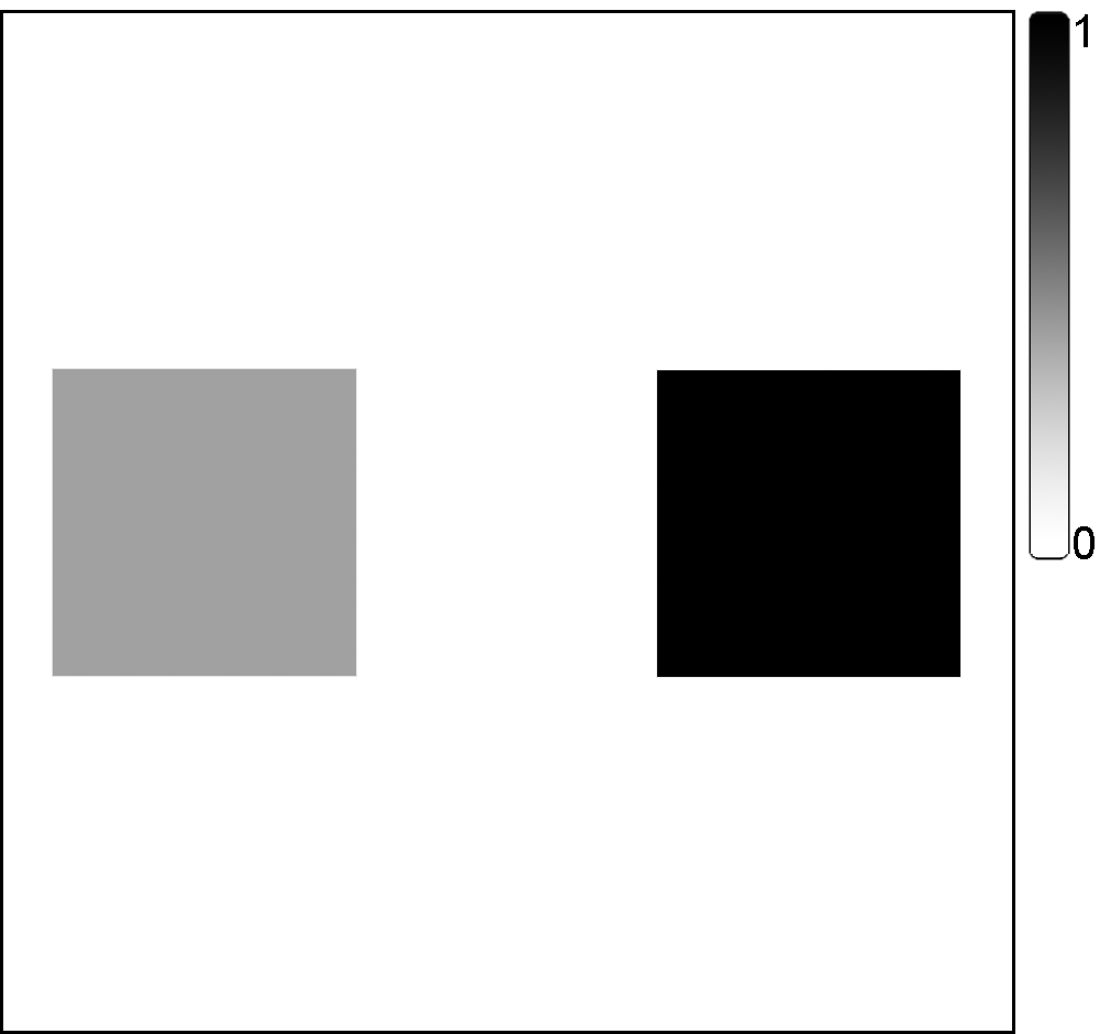
(b) $60<t\leq 120$

Figure 1: Dynamic event density.

Both the random mode and the gradient mode depend on a $\mathit{StepSize}$ parameter. Each step taken by an agent in random mode carries it $\mathit{StepSize}$ distance units in a randomly chosen direction. If in gradient mode, the distance traversed by the agent in the $(\partial F/\partial s_{ix},\partial F/\partial s_{iy})$ direction in one step is $\mathit{StepSize}|(\partial F/\partial s_{ix},\partial F/\partial s_{iy})|$, where $i$ is the agent in question. Note that, unlike what happens in random mode, the distance traversed in one step by agent $i$ in gradient mode can vary with both $s$ and $t$, as it depends on the magnitude of $(\partial F/\partial s_{ix},\partial F/\partial s_{iy})$.

3.2 Saving energy

Whatever energy an agent has left at any time must be used for moving, communicating, and sensing. Even though we do not model energy consumption explicitly, we have striven for our algorithm to be mindful of the agents’ energy usage so that each agent can keep on monitoring its surroundings for events of interest for as long as possible. We let agents do their sensing at all times, but moving and communicating are constrained for the sake of saving energy.

The constraint we impose on an agent’s movements is to allow it to move only once every $\mathit{StillTime}$ time units, regardless of which execution mode it happens to be operating in, where $\mathit{StillTime}$ is a parameter. As mentioned earlier, we assume that $\mathit{StillTime}$ is much greater than the time an agent would spend in a single movement, so agent displacements are assumed to be instantaneous. As for constraining an agent’s ability to communicate to save energy, we assume that whatever information the agent has gathered since last moving is accumulated and sent out in a single message right after it moves next.

3.3 Message handling

Each message contains its sender’s unique identification and current location, as well as all events sensed by the sending agent during the past $\mathit{StillTime}$ time units. Each of these events is represented by the point in $\Omega$ and the time at which it occurred. Upon receiving any such message, and having made sure that originally it was sent out by another agent and is now being received for the first time, an agent passes it on and updates its current view of the system. This view includes node locations and event information, the latter easily kept free of duplicates.

Our derivation in Appendix A leaves it clear that, in order for agent $i$ to compute $\partial F/\partial s_{ix}$ and $\partial F/\partial s_{iy}$ when operating in gradient mode, it must make use of all constituents of its current view, including the locations of agents operating in random mode. However, we know from experience that such locations can be somewhat jittery and thereby contribute to gradient calculation mainly as noise. For this reason, agents operating in random mode always communicate invalid coordinates when sending out their locations. They can then be easily identified by the receiving agents and their locations ignored when computing the gradient of $F$.

3.4 Estimating the event density function

Computing $\partial F/\partial s_{ix}$ and $\partial F/\partial s_{iy}$ also requires agent $i$ to estimate the value of $\phi$ all over $\Omega$ based on a recent time window. At time $t$ this window is given by the interval $[t-\mathit{TimeWindow},t]$, where $\mathit{TimeWindow}$ is another parameter, one that gives rise to a trade-off between how many events can be used to estimate $\phi$ (larger values for $\mathit{TimeWindow}$ are preferable) and how up-to-date $\phi$ can be taken to be (smaller values for $\mathit{TimeWindow}$ are preferable).

In order to handle the spatial dependencies of $\phi$, we subdivide the target region into $\Delta\times\Delta$ cells for suitably chosen $\Delta$ and use a new density function, $\phi^{\prime}$, as a surrogate for $\phi$. The new function is best written as $\phi^{\prime}_{i}(\ell,m,t)$, where $\ell$ and $m$ are nonnegative integers serving to index each cell along the two dimensions and the subscript $i$ is meant to emphasize that $\phi^{\prime}_{i}$ refers to agent $i$’s local estimate of $\phi^{\prime}$. The value of $\phi^{\prime}_{i}(\ell,m,t)$ is computed by first totaling the number of events that according to agent $i$’s current view occurred at some point in cell $(\ell,m)$ during the time interval $[t-\mathit{TimeWindow},t]$, and then normalizing the result over all cells so that the greatest resulting value of $\phi^{\prime}_{i}$ is $1$.

3.5 Switching the execution mode

At time $t=0$ it is impossible to calculate $\phi^{\prime}$ for any cell, so all agents start out in random mode. From then on all agents may switch back and forth between the two execution modes, depending on the event-occurrence pattern they detect at their current locations. This movement between the two modes depends on the current value of $|(\partial F/\partial s_{ix},\partial F/\partial s_{iy})|$, in the case of agent $i$, and on two further parameters, $\mathit{RtoGMinGrad}$ and $\mathit{GtoRMaxGrad}$.

Whenever agent $i$ is up for another move, it computes the magnitude $|(\partial F/\break\partial s_{ix},\partial F/\partial s_{iy})|$ based on its current view of the system. If agent $i$ is currently operating in random mode and the computed magnitude falls strictly above $\mathit{RtoGMinGrad}$, then it switches to gradient mode already for the move it is about to make. If its current mode is the gradient mode and the magnitude falls strictly below $\mathit{GtoRMaxGrad}$, then it switches to random mode.

This is the basic switch policy that agent $i$ follows, but note that it may perpetuate the agent’s operation in gradient mode should it continually encounter sufficiently high event densities. This can be problematic and a case in point is precisely the scenario illustrated above with respect to Figure 1. We help agents avoid such a pitfall by employing yet another parameter, $\mathit{GtoRProb}$, which is the probability with which an agent in gradient mode switches to random mode upon preparing to make a new move even if the relevant gradient components indicate its permanence in gradient mode. Upon switching to random mode, the first $\mathit{GtoRFirstSteps}$ steps are all in the same, randomly chosen direction, $\mathit{GtoRFirstSteps}$ being another parameter. The goal of these first steps is to jump-start the agent on the task of seeking new places to monitor.

4 Computational experiments

In this section we present computational results for a few representative sensing tasks. They were designed to highlight the working of our algorithm’s innermost core, which is the agents’ ability to switch between two execution modes depending on parameter values. Our results are derived from computational simulations carried out for $\Omega$ a $1\,000\times 1\,000$ square and $\Delta=10$, with radii $R_{s}=100$ and $R_{c}=200$. For each specific application, supplementary videos are also provided.

We evaluate our algorithm’s performance through the use of two metrics, both related to the number of events that, throughout the entire simulation, get detected by the agents. Both metrics are significant, but each one’s particular importance in practice depends on the sensing task at hand. They are:

Global fraction of events: The fraction representing how many events were detected by at least one agent.

Average local fraction of events: The average of several fractions, one for each agent, each representing how many events were taken notice of by that specific agent. An agent takes notice of an event by either detecting it directly or receiving it in a message from another agent.

The first of these metrics is of a global character and tends to be higher as more events fall within an agent’s sensing radius. The second metric is of an entirely local nature, since it relates to how the various agents perceive the occurrence of events. This metric tends to be higher as both sensing and communicating are carried out more effectively by the agents. In what follows, these two metrics are always reported as averages (with confidence intervals at the $95\%$ level) over all instants of $200$ independent simulations, each one starting with the agents positioned uniformly at random inside $\Omega$.

Window-based versions of these metrics can be obtained by taking into account only the events detected within a certain time window centered at time $t$. We give plots of these versions in Appendix B, where averages over the $200$ simulations are shown as a function of $t$, again with confidence intervals at the $95\%$ level. These intervals are sometimes quite small, therefore imperceptible in the figures.

In all cases we report results for three distinct agent behaviors regarding the switch between the random mode and the gradient mode, each one controlled by the $\mathit{RtoGMinGrad}$, $\mathit{GtoRMaxGrad}$, and $\mathit{GtoRProb}$ parameters:

Random behavior: This agent behavior occurs when $\mathit{RtoGMinGrad}$ is very large (denoted by $\mathit{RtoGMinGrad}=\infty$) and therefore no agent ever leaves the random mode. This is our control scenario for evaluating how effective gradient-following can be.

Gradient behavior: At the opposing end we have $\mathit{GtoRProb}=0$, in which case an agent can only return to the random mode as a function of the gradient of $F$. Because all agents start out in random mode, this means that any agent encountering sufficient event density for it to switch to gradient mode (as controlled by the $\mathit{RtoGMinGrad}$ parameter) will remain in gradient mode until that density once again becomes insufficient (as controlled by the $\mathit{GtoRMaxGrad}$ parameter).

Mixed behavior: This is the general behavior described in Section 3. It corresponds to setting $\mathit{RtoGMinGrad}$, $\mathit{GtoRMaxGrad}$, and $\mathit{GtoRProb}$ to nonzero finite values.

4.1 Experiment 1: One moving rain cloud

In this experiment, a rain cloud is simulated that moves uniformly from left to right across $\Omega$ as shown in Figure 2. Each of the simulations comprised a total of $900\,000$ events, each one representing the fall of a raindrop on the ground but with $\mathit{VisTime}=0$ (no further visibility, as in the case of a highly porous surface). All parameters are as given in Table 1, results in Table 2. Sample animations are given in supplementary videos for the random (http://www.cos.ufrj.br/ṽalmir/EPB2015-E1-R.mp4), mixed (http://www.cos.ufrj.br/ṽalmir/EPB2015-E1-M.mp4), and gradient (http://www.cos.ufrj.br/ṽalmir/EPB2015-E1-G.mp4) behaviors.

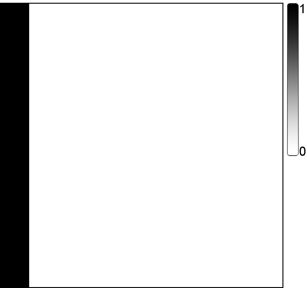
(a) $t=0$

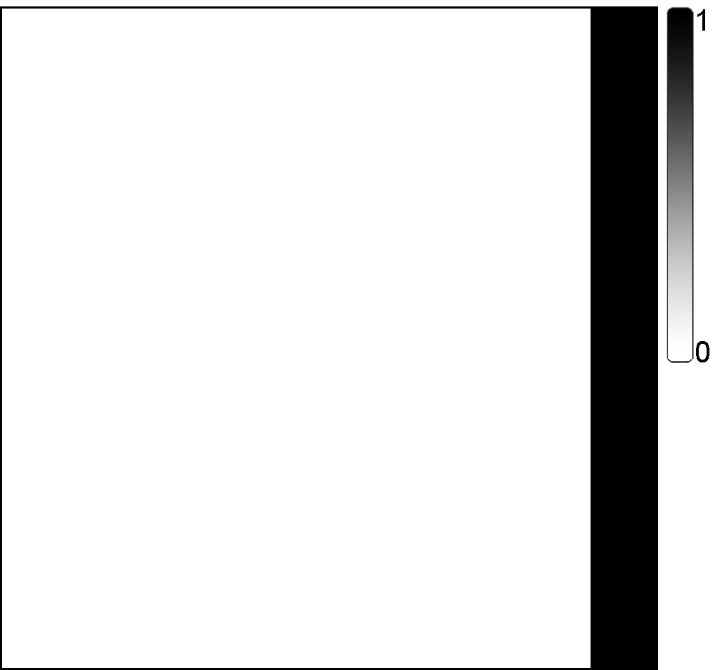
(b) $t=90\,000$

Figure 2: Initial (a) and final (b) event densities for Experiment 1.

Table 1: Parameter values for Experiment 1.

Parameter	Behavior
	Random	Mixed	Gradient
Maximum value of $t$	$90\,000$
$N$	30
$\mathit{StillTime}$	10
$\mathit{RtoGMinGrad}$	$\infty$	0.01	0.01
$\mathit{GtoRMaxGrad}$	$\infty$	0.00001	0.00001
$\mathit{GtoRProb}$	1	0.005	0
$\mathit{GtoRFirstSteps}$	0	10	0
$\mathit{StepSize}$	30
$\mathit{VisTime}$	0
$\mathit{TimeWindow}$	$1\,000$

Table 2: Results for Experiment 1. Confidence intervals correspond to the $95\%$ level.

Metric	Behavior
	Random	Mixed	Gradient
Global fraction of events (%)	$15.0\pm 0.1$	$51.5\pm 0.3$	$76.3\pm 0.1$
Average local fraction of events (%)	$6.8\pm 0.1$	$33.2\pm 0.4$	$72.0\pm 0.3$

No matter which of the two metrics we concentrate on, Table 2 is unequivocal in pointing to the gradient behavior as the one to be chosen. In a situation in which events leave no footprint and moreover occur only on a moving patch inside $\Omega$, the only possibility for agents operating in random mode to come across any event at the time of its occurrence is to chance upon the moving patch and then switch to gradient mode. This explains the superiority of the gradient behavior, followed by the mixed behavior and by the random behavior (this one trailing far behind).

Further examining the figures for the gradient behavior reveals only a small difference between the global metric and the average local one. This means that, while clustering about the moving patch, those agents that do so are capable of efficiently communicating to one another most of what they sense. In the end, on average an agent has been notified of almost all events that got detected by at least one agent.

Additional details can be seen in Figure B.1, where the evolution in time of the window-based versions of the two metrics is shown for this experiment. The metrics’ evolution is mostly uneventful, with values rising toward a certain level and being sustained there throughout the simulation. The one marked exception is that of the window-based local metric when the agents operate under the mixed behavior. In this case, the value that is attained after the initial growth fails to be sustained and begins to undergo a slow decrease. Readily, the farther the rainy patch is from the middle longitudes of $\Omega$, the less effective inter-agent communication becomes. This is so because the distance between the agents actually detecting the events (those operating in gradient mode) and the ones roaming about all of $\Omega$ (those operating in random mode) becomes on average significantly larger.

4.2 Experiment 2: Two moving rain clouds

The setting for this second experiment is similar to that of Experiment 1, the main difference being a second rain cloud that trails the first across $\Omega$, having entered the scene at $t=10\,000$ (Figure 3). The number of events per simulation now totals $1\,650\,000$. Parameter values are given in Table 3, results in Table 4. Sample animations are given in supplementary videos for the random (http://www.cos.ufrj.br/ṽalmir/EPB2015-E2-R.mp4), mixed (http://www.cos.ufrj.br/ṽalmir/EPB2015-E2-M.mp4), and gradient (http://www.cos.ufrj.br/ṽalmir/EPB2015-E2-G.mp4) behaviors.

(a) $t=0$

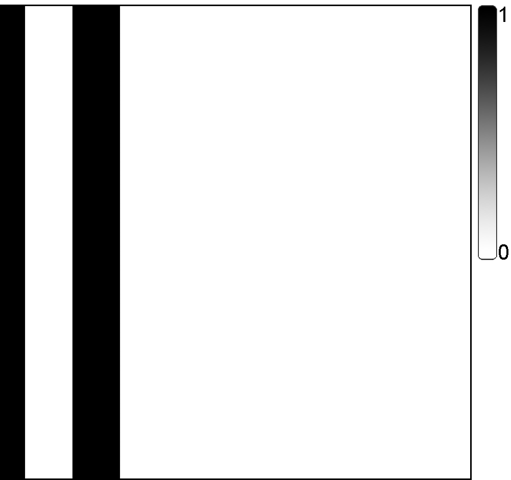
(b) $t=15\,000$

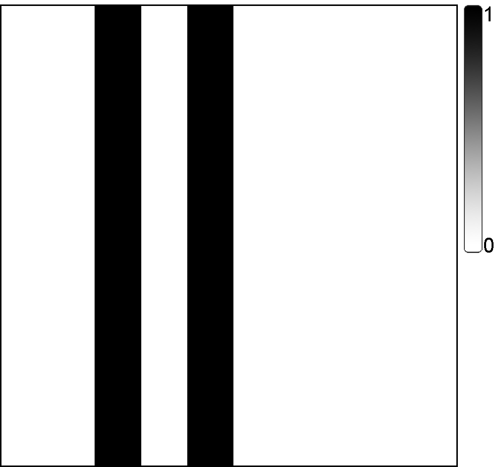
(c) $t=40\,000$

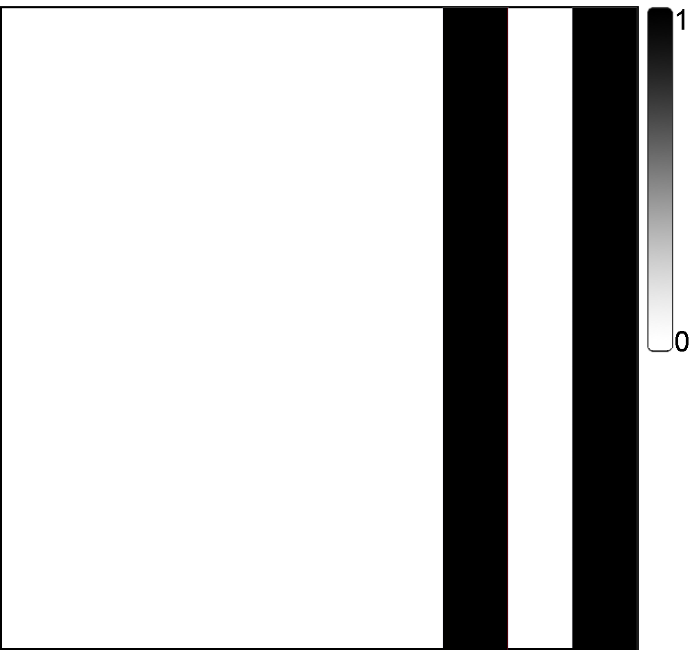
(d) $t=90\,000$

Figure 3: Evolution of the event density for Experiment 2 (a–d).

Comparing the results in Table 4 to those of Table 2 (for Experiment 1) reveals that now agents are better off adopting the mixed (rather than the gradient) behavior. To see why this is so, consider that the appearance of the second rain cloud is challenging to the agents currently concentrating on the first one, in the sense that, in order to reach it, they first have to leave the gradient mode, then cross the dry patch between the two rain clouds, and finally revert to gradient mode once again upon detecting the increase in event density that the second rain cloud entails.

The superiority of the mixed behavior in the case of Experiment 2 holds for the two metrics we have adopted, with the gradient behavior following close behind and the random behavior once again trailing significantly farther back. Moreover, once again it is the case that, for the mixed behavior, the two metrics do not differ greatly and therefore we see that whatever the agents detect is nearly as effective locally as it is globally. In the case of Experiment 2, this is true of the gradient behavior as well.

Table 3: Parameters values for Experiment 2.

Parameter	Behavior
	Random	Mixed	Gradient
Maximum value of $t$	$90\,000$
$N$	30
$\mathit{StillTime}$	10
$\mathit{RtoGMinGrad}$	$\infty$	0.01	0.01
$\mathit{GtoRMaxGrad}$	$\infty$	0.00001	0.00001
$\mathit{GtoRProb}$	1	0.0005	0
$\mathit{GtoRFirstSteps}$	0	10	0
$\mathit{StepSize}$	30
$\mathit{VisTime}$	0
$\mathit{TimeWindow}$	$1\,000$

Table 4: Results for Experiment 2. Confidence intervals correspond to the $95\%$ level.

Metric	Behavior
	Random	Mixed	Gradient
Global fraction of events (%)	$14.9\pm 0.1$	$50.1\pm 0.2$	$41.5\pm 0.1$
Average local fraction of events (%)	$6.9\pm 0.1$	$44.8\pm 0.3$	$39.1\pm 0.1$

Still in comparison to the data for Experiment 1, it is worth noting that figures are now significantly lower under the gradient behavior (this, in fact, is why in Experiment 2 the mixed behavior rose to the top). The reason for this, clearly, is that while in the gradient behavior agents neglect the second rain cloud altogether, thence the ensuing drop in their performance.

Additional insight can be gained by examining the evolution in time of the window-based versions of the two metrics (Figure B.2). Clearly, up until $t=10\,000$ (the time of appearance of the second rain cloud), the agents’ performances in either of the two gradient-based behaviors are indistinguishable. Between this time and that at which the second wet patch becomes fully contained in $\Omega$, performance under these two behaviors undergoes a significant drop. Afterwards the mixed behavior succeeds in gradually leading the system to some degree of recovery from the drop while the gradient behavior does not.

4.3 Experiment 3: Persistent pollutants

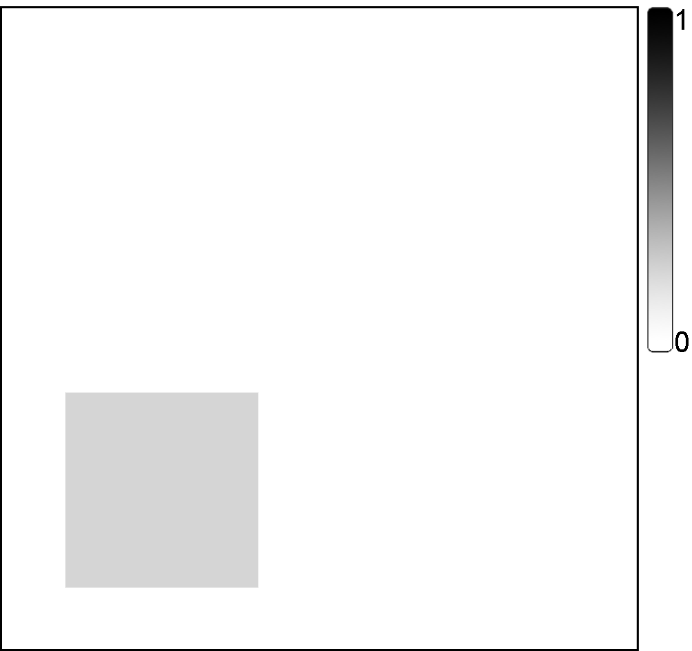
(a) $0\leq t\leq 25\,000$

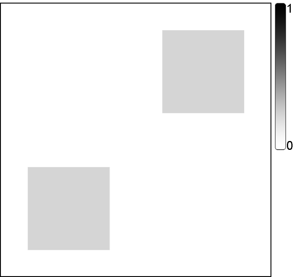
(b) $25\,000<t\leq 50\,000$

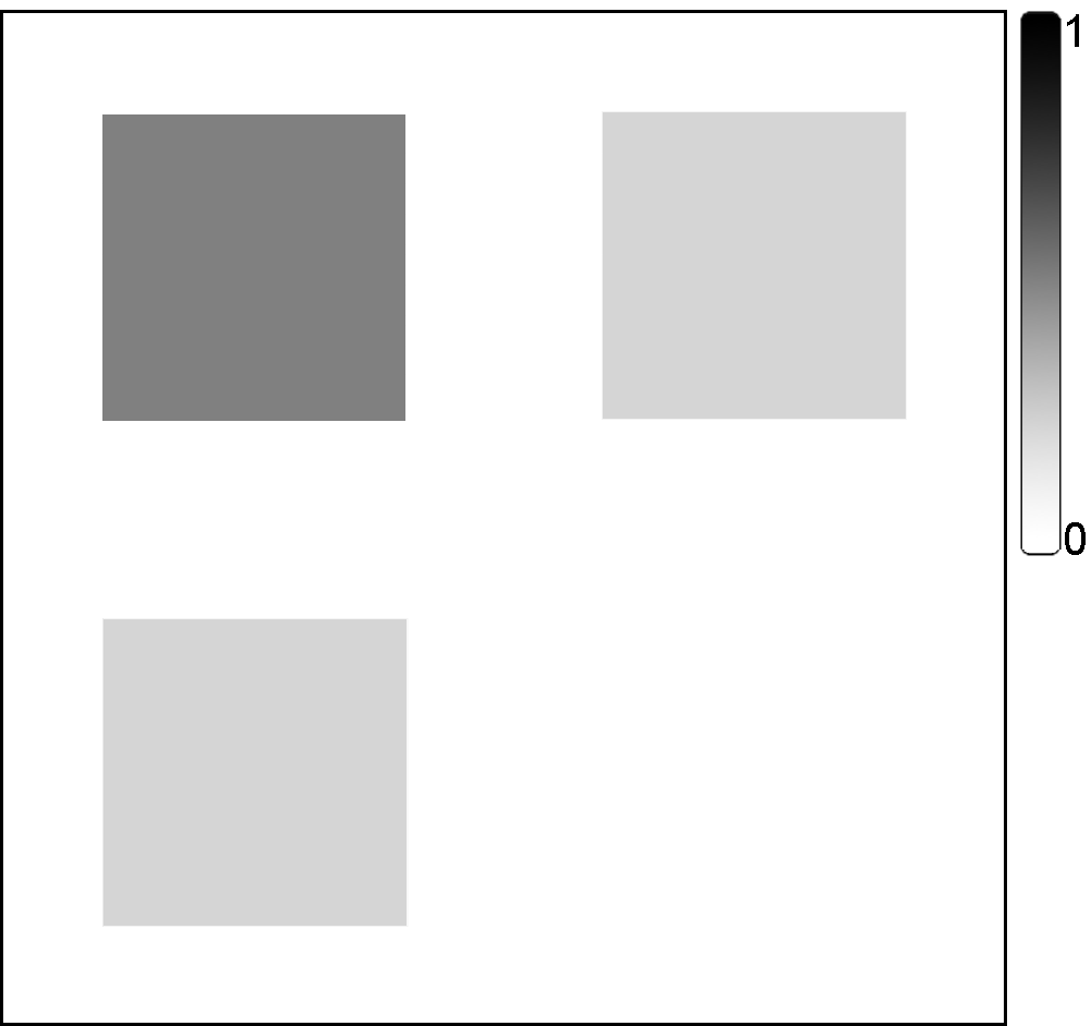
(c) $50\,000<t\leq 75\,000$

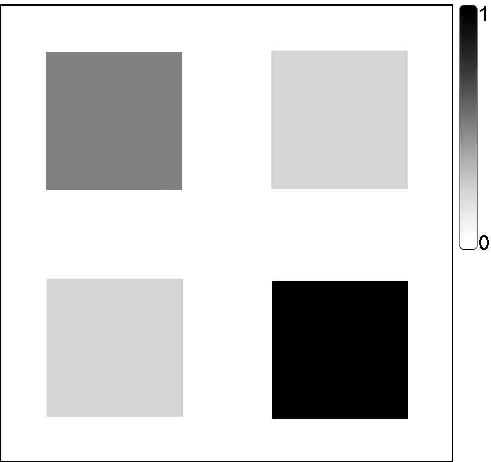
(d) $75\,000<t\leq 100\,000$

Figure 4: Evolution of the event density for Experiment 3 (a–d).

Table 5: Parameter values for Experiment 3.

Parameter	Behavior
	Random	Mixed	Gradient
Maximum value of $t$	$100\,000$
$N$	50
$\mathit{StillTime}$	20
$\mathit{RtoGMinGrad}$	$\infty$	0.01	0.01
$\mathit{GtoRMaxGrad}$	$\infty$	0.00001	0.00001
$\mathit{GtoRProb}$	1	0.01	0
$\mathit{GtoRFirstSteps}$	0	10	0
$\mathit{StepSize}$	25
$\mathit{VisTime}$	100
$\mathit{TimeWindow}$	$1\,000$

Table 6: Results for Experiment 3. Confidence intervals correspond to the $95\%$ level.

Metric	Behavior
	Random	Mixed	Gradient
Global fraction of events (%)	$57.5\pm 0.2$	$80.6\pm 0.2$	$45.3\pm 0.3$
Average local fraction of events (%)	$51.8\pm 0.3$	$59.7\pm 0.4$	$24.5\pm 0.1$

This experiment continues the trend initiated by Experiment 2 in that events are concentrated in more than one patch inside $\Omega$ and moreover new patches appear as time elapses. The two settings differ, though, mainly in that the event patches no longer move, but also in that they now appear more abruptly and also with different event densities, totaling $750\,000$ events (Figure 4). The new experiment also sets $\mathit{VisTime}=100$, the metaphor now being that of pollutant particles that stick to the environment and therefore have a nonzero visibility time. The parameter values used are those shown in Table 5. We give results in Table 6. Sample animations are given in supplementary videos for the random (http://www.cos.ufrj.br/ṽalmir/EPB2015-E3-R.mp4), mixed (http://www.cos.ufrj.br/ṽalmir/EPB2015-E3-M.mp4), and gradient (http://www.cos.ufrj.br/ṽalmir/EPB2015-E3-G.mp4) behaviors.

The most striking figures in Table 6 are those for the random behavior, which not only surpass those of the previous experiments by a great margin but also put random behavior ahead of gradient behavior. The main reason for this seems clear: given that the event patches remain spatially static once they appear, the freely roaming agents in random mode eventually succeed in detecting a sizable fraction of the events, even if they cover the denser patches somewhat thinly.

Other interesting data in the table are those referring to the agents’ performance under the gradient behavior. In this case they fare worse than they do under random behavior, and again the reason seems clear: as denser patches continue to crop up, those agents not yet involved with monitoring the already existing patches will tend to be too few, certainly fewer than necessary to provide the new patches with any degree of satisfactory coverage.

Given these explanations for the agents’ performance under the random behavior and the gradient behavior, it should be no surprise that, as in Experiment 2, once again the mixed behavior is the best option. Its mixed nature seems to alleviate the shortcomings of the other two behaviors, much as it strengthens their advantages. Note, additionally, that in the two behaviors involving any participation of the gradient mode the local metrics are valued significantly below the global one. What seems to be happening is that, because of the patches’ spatial separation from one another, effectively conveying sensing information from agents at one patch to those at another depend more on agents operating in random mode than it would otherwise do.

The evolution in time of the window-based metrics, shown in Figure B.3, provides further valuable information. As in the case of Experiment 2, the appearance of each new, spatially separated patch of events causes significant drops in performance when the agents are in either of the two gradient-based behaviors. Recovery always follows under the mixed behavior, though to somewhat lower levels, which eventually guarantees its overall superiority. As for the gradient behavior, some recovery also takes place but is severely insufficient to lead to any significant level of overall performance. In particular, such recovery only happens while there exist agents operating in random mode, which is reflected in the complete absence of any recovery from the appearance of the new event patches right past $t=50\,000$ and $t=75\,000$.

5 Conclusion

We have introduced a new distributed algorithm for a collection of mobile agents to monitor a two-dimensional domain seeking to sense and possibly store events of a certain nature occurring in their target region. The algorithm is fully distributed, in the sense that not even leader agents are needed, and is also fully adaptive, in the sense that it strives for agents to perform well in their sensing tasks even if the events in question vary both spatially and temporally. At the heart of the algorithm lies the notion of an execution mode, of which there are two (the random mode and the gradient mode), which in essence is a pattern of behavior allowing the agent to concentrate on certain specific aspects of the monitoring task to be carried out.

Agents operating in random mode are tailored to handle the uncertainties of some situations, such as those in which events tend to happen unpredictably. Those operating in gradient mode find guidance in the locally perceived density of events to move toward points that may surround their current locations having higher values of a density-dependent function. Depending on a variety of parameters whose setting in turn depends on the specific application at hand, agents are capable of switching back and forth between the two execution modes and thereby help the system as a whole profit as much as possible from each mode’s characteristics.

We illustrated some of this interplay of parameter values by means of three computational experiments, each one designed to highlight those aspects of an application that justify the spectrum of behaviors we called random, mixed, and gradient. Such aspects include the occurrence of events whose spatial coordinates vary with time, both within a connected portion of the target region and otherwise; the rapid change in the overall event density across spatially separated portions of the target region; and some of the peculiarities of an event’s environmental footprint.

Our solution has been given for the case of a two-dimensional target region but nothing prevents its straightforward extension to three dimensions, provided only that the agents themselves can exist and move in a three-dimensional setting. It would also be straightforward to adopt sensing and communication models more realistic than those of Eqs. (1) and  (2), respectively. In a similar vein, and notwithstanding its already large set of parameters, endowing the algorithm with even more parameters should not be out of the question. In fact, the ability to have so many of its details adjustable is precisely what makes it potentially applicable to a wide variety of situations.

Acknowledgments

The authors acknowledge partial support from CNPq, CAPES, and a FAPERJ BBP grant.

Appendix A Computing the gradient

We first rewrite Eq. (4) for fixed $t$ as

$$F(s)=\int_{\Omega}\phi(q)\mathrm{d}q-\int_{\Omega}\phi(q)\prod_{k=1}^{N}[1-p_{k}(q)]\mathrm{d}q.$$ (A.1)

Then we proceed by differentiating $F$ with respect to $s_{ix}$, which yields

$$\frac{\partial F}{\partial s_{ix}}=-\int_{\Omega_{i}}\phi(q)\prod_{{k=1}\atop{k\neq i}}^{N}[1-p_{k}(q)]\frac{\partial}{\partial s_{ix}}[1-p_{i}(q)]\mathrm{d}q,$$ (A.2)

where $\Omega_{i}$ is the intersection of $\Omega$ with the radius-$R_{s}$ circle centered at $s_{i}=(s_{ix},s_{iy})$. This follows from the fact that $p_{i}(q)$ does not depend on $s_{ix}$ for $q\in\Omega\setminus\Omega_{i}$, by Eq. (1). By the same token, noting further that $p_{k}(q)=0$ whenever $\Omega_{k}\cap\Omega_{i}=\emptyset$ leads to

$$\frac{\partial F}{\partial s_{ix}}=-\int_{\Omega_{i}}\phi(q)\prod_{{{k=1}\atop{k\neq i}}\atop{\Omega_{k}\cap\Omega_{i}\neq\emptyset}}^{N}[1-p_{k}(q)]\frac{\partial}{\partial s_{ix}}[1-p_{i}(q)]\mathrm{d}q.$$ (A.3)

Using $q=(q_{x},q_{y})$, and recalling that $d_{i}=[(s_{ix}-q_{x})^{2}+(s_{iy}-q_{y})^{2}]^{1/2}$, we obtain

$$\frac{\partial p_{i}}{\partial s_{ix}}=\frac{2(s_{ix}-q_{x})}{R_{s}}\left(\frac{1}{R_{s}}-\frac{1}{d_{i}}\right)$$ (A.4)

and

$$\frac{\partial F}{\partial s_{ix}}=\int_{\Omega_{i}}\phi(q)\prod_{{{k=1}\atop{k\neq i}}\atop{\Omega_{k}\cap\Omega_{i}\neq\emptyset}}^{N}[1-p_{k}(q)]\frac{2(s_{ix}-q_{x})}{R_{s}}\left(\frac{1}{R_{s}}-\frac{1}{d_{i}}\right)\mathrm{d}q.$$ (A.5)

As explained in Section 3.4, for use in the algorithm by agent $i$ in relation to time $t$, subdividing $\Omega$ into the square cells of side $\Delta$ while $\phi^{\prime}_{i}$ substitutes for $\phi$ requires an approximation to the above expression for $\partial F/\partial s_{ix}$. Using $q=(q_{\ell},q_{m})$ as the central point of cell $(\ell,m)$ leads to the discrete approximation

$$\frac{\partial F}{\partial s_{ix}}\approx\sum_{\ell}\sum_{m}\phi^{\prime}_{i}(\ell,m,t)\prod_{{{k=1}\atop{k\neq i}}\atop{\Omega_{k}\cap\Omega_{i}\neq\emptyset}}^{N}[1-p_{k}(q)]\frac{2(s_{ix}-q_{x})}{R_{s}}\left(\frac{1}{R_{s}}-\frac{1}{d_{i}}\right),$$ (A.6)

where $\ell$ and $m$ range over the cells that intersect $\Omega_{i}$ and $d_{i}=[(s_{ix}-q_{\ell})^{2}+(s_{iy}-q_{m})^{2}]^{1/2}$.

The case of $\partial F/\partial s_{iy}$ is entirely analogous and yields

$$\frac{\partial F}{\partial s_{iy}}\approx\sum_{\ell}\sum_{m}\phi^{\prime}_{i}(\ell,m,t)\prod_{{{k=1}\atop{k\neq i}}\atop{\Omega_{k}\cap\Omega_{i}\neq\emptyset}}^{N}[1-p_{k}(q)]\frac{2(s_{iy}-q_{y})}{R_{s}}\left(\frac{1}{R_{s}}-\frac{1}{d_{i}}\right).$$ (A.7)

Appendix B Additional figures

The figures in this appendix accompany the discussion in Section 4. They refer to the window-based versions of the two metrics introduced in that section.

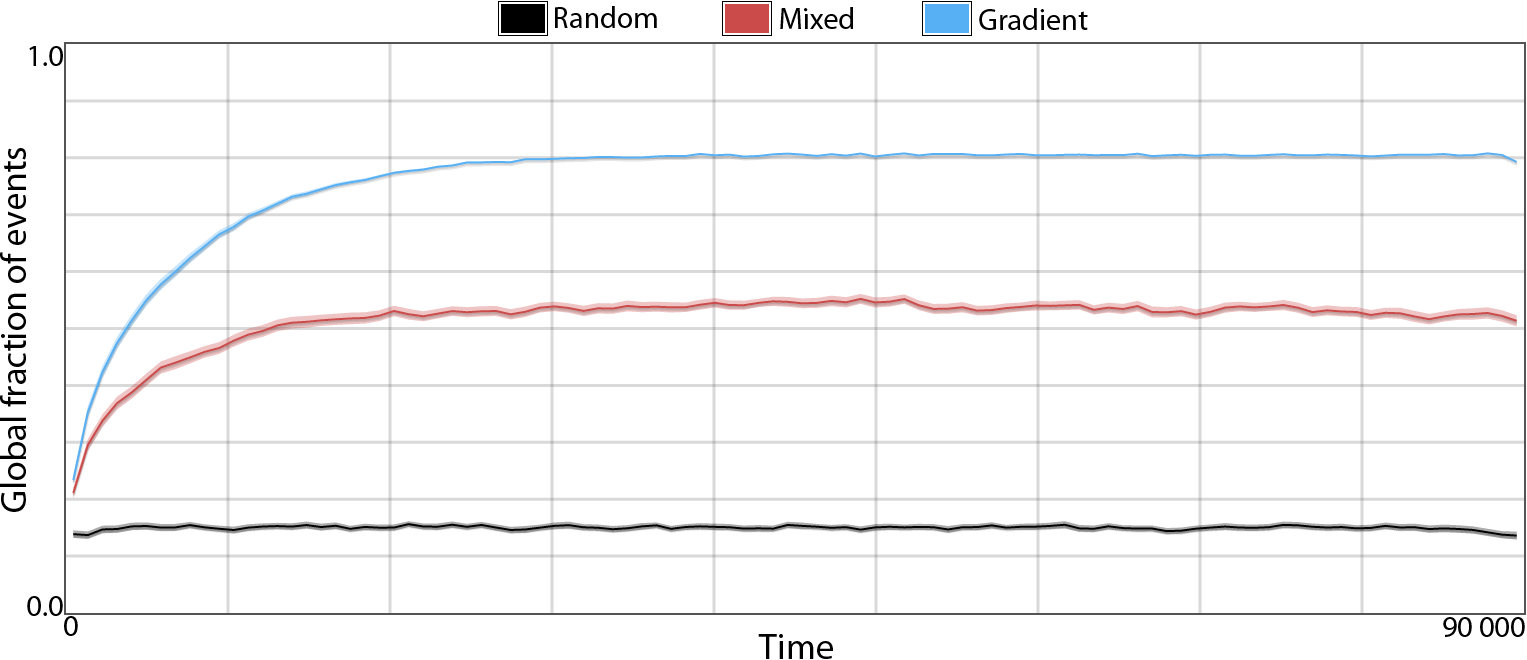
(a)

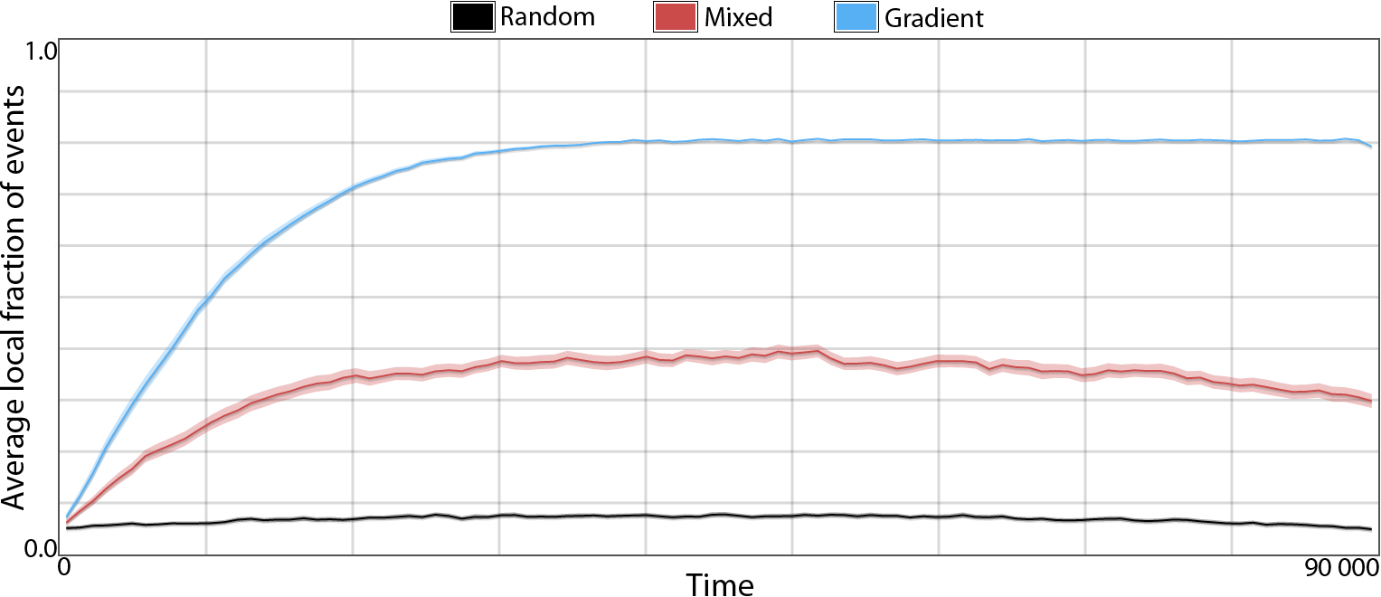
(b)

Figure B.1: Evolution in time of the average global (a) and local (b) window-based metrics for Experiment 1. Window size is $900$. Confidence intervals correspond to the $95\%$ level.

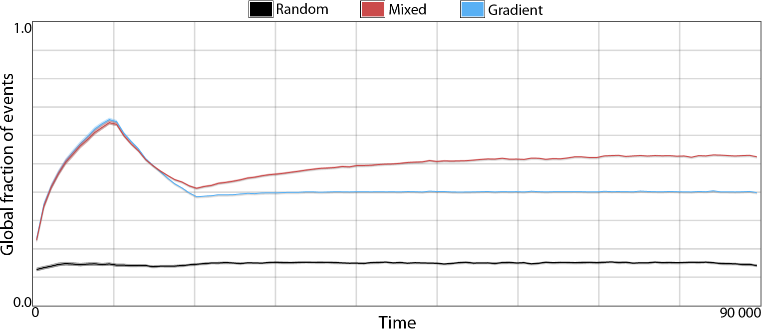
(a)

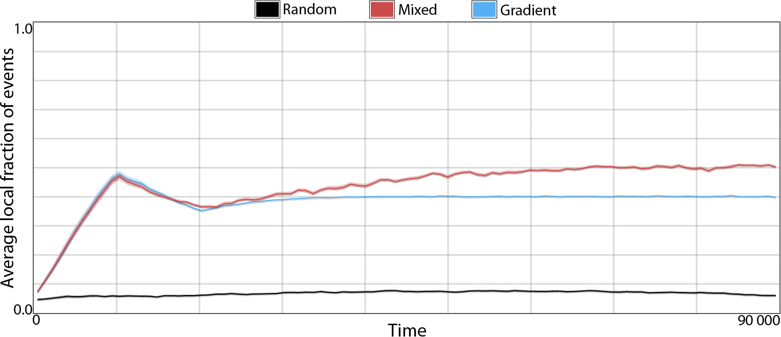
(b)

Figure B.2: Evolution in time of the average global (a) and local (b) window-based metrics for Experiment 2. Window size is $900$. Confidence intervals correspond to the $95\%$ level.

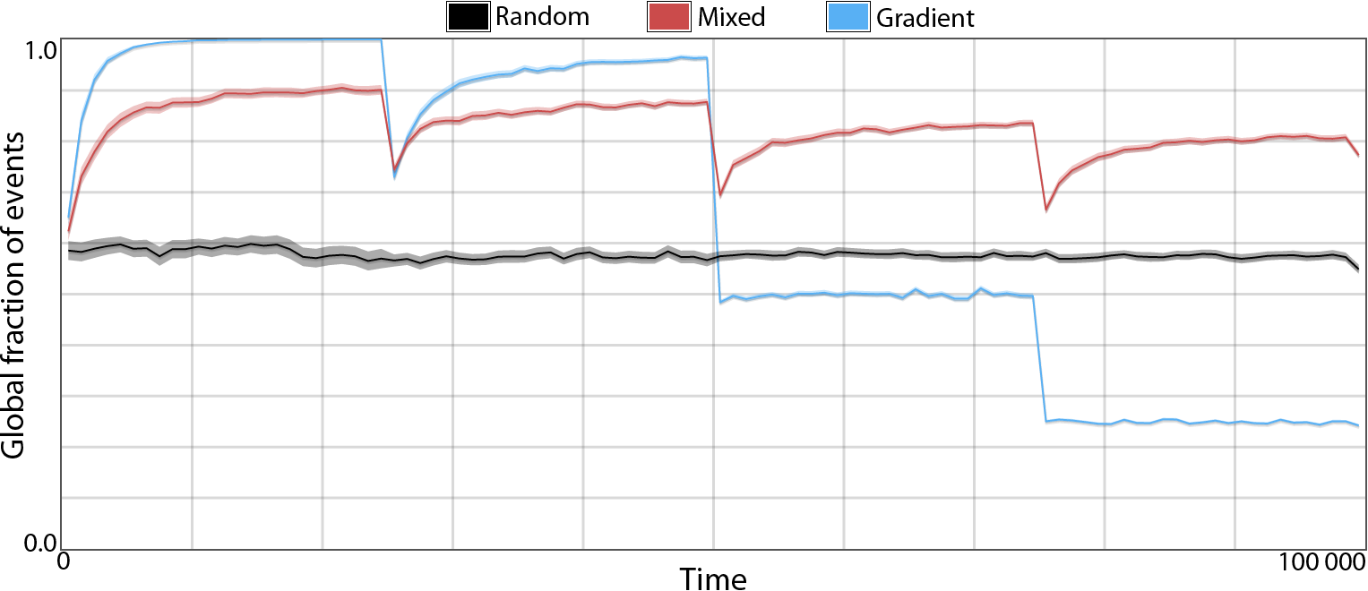
(a)

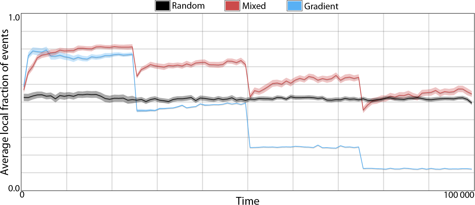
(b)

Figure B.3: Evolution in time of the average global (a) and local (b) window-based metrics for Experiment 3. Window size is $1\,000$. Confidence intervals correspond to the $95\%$ level.

References

- [1] A. Gusrialdi, R. Dirza, and S. Hirche. Information-driven distributed coverage algorithms for mobile sensor networks. In Proc. ICNSC, pages 242–247, 2011.
- [2] S. Martinez, J. Cortes, and F. Bullo. Motion coordination with distributed information. IEEE Contr. Syst. Mag., 27(4):75–88, 2007.
- [3] Andrew Howard, Majai J. Matarić, and Gaurav S. Sukhatme. Mobile sensor network deployment using potential fields: a distributed, scalable solution to the area coverage problem. In Hajime Asama, Tamio Arai, Toshio Fukuda, and Tsutomu Hasegawa, editors, Distributed Autonomous Robotic Systems 5, pages 299–308. Springer-Verlag, Tokyo, Japan, 2002.
- [4] Y. Zou and Krishnendu Chakrabarty. Sensor deployment and target localization based on virtual forces. In Proc. INFOCOM, pages 1293–1303, 2003.
- [5] Wei Li and C. G. Cassandras. Distributed cooperative coverage control of sensor networks. In Proc. CDC-ECC, pages 2542–2547, 2005.
- [6] M. J. Nene, R. S. Deodhar, and L. M. Patnaik. UREA: Uncovered Region Exploration Algorithm for reorganization of mobile sensor nodes to maximize coverage. In Proc. DCOSSW, pages 1–6, 2010.
- [7] A. Gusrialdi, R. Dirza, T. Hatanaka, and M. Fujita. Improved distributed coverage control for robotic visual sensor network under limited energy storage. Int. J. Imag. Robot., 10(2):58–74, 2013.
- [8] Cheng Song, Lu Liu, Gang Feng, and Yuan Fan. Persistent awareness coverage with maximum coverage frequency for mobile sensor networks. In Proc. IEEE-CYBER, pages 235–240, 2013.
- [9] Meng Ji and M. Egersted. A graph-theoretic characterization of controllability for multi-agent systems. In Proc. ACC, pages 4588–4593, 2007.
- [10] M. Penrose. Random Geometric Graphs. Oxford University Press, Oxford, UK, 2003.
- [11] Y. Peres, A. Sinclair, P. Sousi, and A. Stauffer. Mobile geometric graphs: detection, coverage and percolation. Probab. Theory Rel., 156:273–305, 2013.