1. Introduction

1.1. Problem formulation and outline of solution strategy

This note describes a direct solver for elliptic PDEs with variable coefficients, such as, e.g.,

(1) $$\left\{\begin{aligned} \mbox{}[Au](\bm{x})=&\ g(\bm{x}),\qquad&\bm{x}\in\Omega,\\ u(\bm{x})=&\ f(\bm{x}),\qquad&\bm{x}\in\Gamma,\end{aligned}\right.$$

where $A$ is a variable coefficient elliptic differential operator

(2) $$[Au](\bm{x})=-c_{11}(\bm{x})[\partial_{1}^{2}u](\bm{x})-2c_{12}(\bm{x})[\partial_{1}\partial_{2}u](\bm{x})-c_{22}(\bm{x})[\partial_{2}^{2}u](\bm{x})\\ +c_{1}(\bm{x})[\partial_{1}u](\bm{x})+c_{2}(\bm{x})[\partial_{2}u](\bm{x})+c(\bm{x})\,u(\bm{x}),$$

where $\Omega$ is a box in the plane with boundary $\Gamma=\partial\Omega$, where all coefficient functions ($c$, $c_{i}$, $c_{ij}$) are smooth, and where $f$ and $g$ are given functions. (For generalizations, see Section 1.4.) The solver is structured as follows:

1. The domain is first tessellated into a hierarchical tree of patches. For each patch on the finest level, a reduced model that we call a “proxy” that represents its internal structure is computed. The proxy takes the form of a dense matrix (that may be stored in a data sparse format), and is for the small patches computed by brute force.

2. The larger patches are processed in an upwards pass through the tree. For each patch, its proxy matrix is formed by merging the proxies of its children.

3. Once the proxies for all patches have been computed, a solution to the PDE can be computed via a downwards pass through the tree. This step is typically very fast.

We observe that this pattern is similar to the classical nested dissection method of George [5], with a large subsequent literature on “multifrontal solver,” see, e.g., [4, 3] and the references therein.

The techniques described in this note are drawn from [12, 13, 7, 6], which in turn is inspired by earlier work on multidomain spectral methods, see, e.g., [14, 11] and the references therein.

1.2. Dirichlet-to-Neumann maps

In this section, the internal structure of a patch is represented by computing its Dirichlet-to-Neumann, or “DtN,” map. To explain what this map does, first observe that for a given boundary function $f$, the BVP (1) typically has a unique solution $\phi$ (unless the operator $A$ happens to have a non-trivial null-space, see Remark 1). Now simply form the boundary function $h$ that gives the normal derivative of the solution,

$$h(\bm{x})=\phi_{n}(\bm{x}),\qquad\bm{x}\in\Gamma,$$

where $\phi_{n}$ is the outwards pointing normal derivative. The process for constructing the function $h$ from $f$ is linear, and we write it as

$$h=T\,f.$$

Or, equivalently,

$$T\,\colon\,\phi|_{\Gamma}\mapsto\phi_{n}|_{\Gamma},\qquad\qquad\mbox{where}\ \phi\ \mbox{satisfies}\ A\phi=0.$$

In general, the map $T$ is a slightly unpleasant object; it behaves as a differentiation operator, and it has complicated singular behavior near the corners of $\Gamma$. A key observation is that in the present context, all these difficulties can be ignored since we limit attention to functions that are smooth. In a sense, we only need to accurately represent the projection of the “true” operator $T$ onto a space of smooth functions (that in particular do not have any corner singularities).

We represent boundary functions by tabulating their values at interpolation nodes on the edges of the boxes. For instance, for a leaf box, we place $q$ Gaussian nodes on each side (for say $q=20$), which means that the functions $f$ and $h$ are represented by vectors $\bm{\mathsf{f}},\bm{\mathsf{h}}\in\mathbb{R}^{4q}$ and the discrete approximation to $T$ is a $4q\times 4q$ matrix $\bm{\mathsf{T}}$. The technique for computing $\bm{\mathsf{T}}$ for a leaf box is described in Section 3. For a parent box $\tau$ with children $\alpha$ and $\beta$, there is a technique for computing $\bm{\mathsf{T}}^{\tau}$ from the matrices $\bm{\mathsf{T}}^{\alpha}$ and $\bm{\mathsf{T}}^{\beta}$ that is described in Section 4. In essence, the idea is simply to enforce continuity of both potentials and fluxes across the edge that is shared by $\Omega_{\alpha}$ and $\Omega_{\beta}$.

Remark 1.

For a general BVP like (1), the DtN operator need not exist. For example, suppose $-k^{2}$ is an eigenvalue of $\Delta$ with zero Dirichlet data. Then the operator $Au=\Delta u+k^{2}u$ clearly has a non-trivial null-space. However, this situation is in some sense “unusual” (since the spectrum of an elliptic PDO on a bounded domain typically is discrete), and it turns out that one can for the most part completely ignore this complication and assume that the DtN operator always exists. Note for instance that if $A$ is coercive (e.g. if $A=-\Delta$), then the DtN is guaranteed to exist for any bounded domain. For problems for which resonances do present numerical problems, there is a variation of the proposed method that is rock-solid stable. The idea is to build a hierarchy of so called impedance maps (instead of DtN maps). These are cousins of the DtN that are defined by

$$R\,\colon\,(\phi+\mathrm{i}\phi_{n})|_{\Gamma}\mapsto(\phi-\mathrm{i}\phi_{n})|_{\Gamma},\qquad\qquad\mbox{where}\ \phi\ \mbox{satisfies}\ A\phi=0.$$

The map $R$ always exists, and is moreover a unitary operator. This construction was proposed by Alex Barnett of Dartmouth College [7].

1.3. Complexity of the direct solver

The asymptotic complexity of the solver described in this note is exactly the same as that for classical nested dissection [5]. For a domain with $N$ interior discretization nodes, the pre-computation (the upwards pass) costs $O(N^{1.5})$ operations, and then the solve (the downwards pass) costs $O(N\log N)$ operations, see [13, Sec. 5.2].

Optimal $O(N)$ complexity can be achieved for both the pre-computation and the solve stage when the Green’s function of the BVP is non-oscillatory. In this case, the matrices $\bm{\mathsf{T}}^{\tau}$ that approximate the DtN operators have enough internal structure that they can be well represented using a data-sparse format such as, e.g., the $\mathcal{H}$-matrix framework of Hackbusch and co-workers [9, 8, 1, 2], see [6].

1.4. Generalizations

For notational simpliticy, this note treats only the simple Dirichlet problem (1). The scheme can with trivial modifications be applied to more general elliptic operators coupled with Dirichlet, Neumann, or mixed boundary data. It has for instance been successfully tested on convection-diffusion problems that are strongly dominated (by a factor of $10^{4}$) by the convection term. It has also been tested on vibration problems modeled by a variable coefficient Helmholtz equation, and has proven capable of solving problems on domains of size $200\times 200$ wavelengths or more on an office laptop computer. The solutions are computed to seven correct digits. Extension to more general domains is done via parameter maps to a rectangle, or union of rectangles. See [13] for details.

1.5. Outline

To keep the presentation uncluttered, we start by describing a direct solver for (1) for the case of no body-load, $g=0$, and with $\Omega=[0,1]^{2}$ the unit square. Section 2 introduces the discretization, and how we represent the approximation to the solution $u$ for (1). Section 3 describes the how to compute the DtN operator for a leaf in the tree. Section 4 describes the merge process for how to take the DtN operators for two touching boxes, and computing the DtN operator for their union. Section 5 describes the full hierarchical scheme. Section 6 describes how to solve a problem with body loads.

2. Discretization

Partition the domain $\Omega$ into a collection of square (or possibly rectangular) boxes, called leaf boxes. On the edges of each leaf, place $q$ Gaussian interpolation points. The size of the leaf boxes, and the parameter $q$ should be chosen so that any potential solution $u$ of (1), as well as its first and second derivatives, can be accurately interpolated from their values at these points ($q=20$ is often a good choice). Let $\{\bm{x}_{k}\}_{k=1}^{N}$ denote the collection of interpolation points on all boundaries.

Next construct a binary tree on the collection of leaf boxes by hierarchically merging them, making sure that all boxes on the same level are roughly of the same size, cf. Figure 1. The boxes should be ordered so that if $\tau$ is a parent of a box $\sigma$, then $\tau<\sigma$. We also assume that the root of the tree (i.e. the full box $\Omega$) has index $\tau=1$. We let $\Omega_{\tau}$ denote the domain associated with box $\tau$.

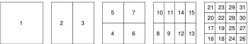
Figure 1. The square domain $\Omega$ is split into $4\times 4$ leaf boxes. These are then gathered into a binary tree of successively larger boxes as described in Section 5.1. One possible enumeration of the boxes in the tree is shown, but note that the only restriction is that if box $\tau$ is the parent of box $\sigma$, then $\tau<\sigma$.

With each box $\tau$, we define two index vectors $I_{\rm i}^{\tau}$ and $I_{\rm e}^{\tau}$ as follows:

• A list of all exterior nodes of $\tau$. In other words, $k\in I_{\rm e}^{\tau}$ iff $\bm{x}_{k}$ lies on the boundary of $\Omega_{\tau}$.

• For a parent $\tau$, $I_{\rm i}^{\tau}$ is a list of all its interior nodes that are not interior nodes of its children. For a leaf $\tau$, $I_{\rm i}^{\tau}$ is empty.

Let $\bm{\mathsf{u}}\in\mathbb{R}^{N}$ denote a vector holding approximations to the values of $u$ of (1), in other words,

$$\bm{\mathsf{u}}(k)\approx u(\bm{x}_{k}).$$

Finally, let $\bm{\mathsf{v}}\in\mathbb{R}^{N}$ denote a vector holding approximations to the boundary fluxes of the solution $u$ of (1), in other words

$$\bm{\mathsf{v}}(k)\approx\left\{\begin{aligned} \partial_{2}u(\bm{x}_{k}),\qquad&\mbox{when }\bm{x}_{j}\mbox{ lies on a horizontal edge,}\\ \partial_{1}u(\bm{x}_{k}),\qquad&\mbox{when }\bm{x}_{j}\mbox{ lies on a vertical edge.}\end{aligned}\right.$$

Note the sign convention for the normal derivatives: we use a global frame of reference, as opposed to distinguishing between outwards and inwards pointing normal derivatives. This is a deliberate choice to avoid problems with signs when matching fluxes of touching boxes.

3. Constructing the Dirichlet-to-Neumann map for a leaf

This section describes a spectral method for computing a discrete approximation to the DtN map $T^{\tau}$ associated with a leaf box $\Omega_{\tau}$. In other words, if $u$ is a solution of (1), we seek a matrix $\bm{\mathsf{T}}^{\tau}$ of size $4q\times 4q$ such that

(3) $$\begin{array}[]{ccccc}\bm{\mathsf{v}}(I_{\rm e}^{\tau})&\approx&\bm{\mathsf{T}}^{\tau}&\bm{\mathsf{u}}(I_{\rm e}^{\tau}).\\ \mbox{{Neumann data}}&&\mbox{{DtN map}}&\mbox{{Dirichlet data}}\end{array}$$

Conceptually, we proceed as follows: Given a vector $\bm{\mathsf{u}}(I_{\rm e}^{\tau})\in\mathbb{R}^{4q}$ specifying the solution $u$ on the boundary of $\Omega_{\tau}$, form for each side the unique polynomial of degree at most $q-1$ that interpolates the $q$ specified values of $u$. This yields Dirichlet boundary data on $\Omega_{\tau}$ in the form of four polynomials. Solve the restriction of (1) to $\Omega_{\tau}$ for the specified boundary data using a spectral method on a local tensor product grid of $p\times p$ Chebyshev nodes (typically, we choose $p=q+1$). The vector $\bm{\mathsf{v}}(I_{\rm e}^{\tau})$ is obtained by spectral differentiation of the local solution, and then re-tabulating the boundary fluxes to the Gaussian nodes in $\{\bm{x}_{k}\}_{k\in I_{\rm e}^{\tau}}$.

We give details of the construction in Section 3.2, but as a preliminary step, we first review a classical spectral collocation method for the local solve in Section 3.1

Remark 2.

Chebyshev nodes are ideal for the leaf computations, and it is in principle also possible to use Chebyshev nodes to represent all boundary-to-boundary “solution operators” such as, e.g., $\bm{\mathsf{T}}^{\tau}$ (indeed, this was the approach taken in the first implementation of the proposed method [13]). However, there are at least two substantial benefits to using Gaussian nodes that justify the trouble to retabulate the operators. First, the procedure for merging boundary operators defined for neighboring boxes is much cleaner and involves less bookkeeping since the Gaussian nodes do not include the corner nodes. (Contrast Section 4 of [13] with Section 4.) Second, and more importantly, the use of the Gaussian nodes allows for interpolation between different discretizations. Thus the method can easily be extended to have local refinement when necessary, see Remark 4.

3.1. Spectral discretization

Let $\Omega_{\tau}$ denote a rectangular subset of $\Omega$ with boundary $\Gamma_{\tau}$, and consider the local Dirichlet problem with the boundary data given by a “dummy” function $\psi$

(4) $$\left\{\begin{aligned} \mbox{}[Au](\bm{x})=&\ 0,\qquad&\bm{x}\in\Omega_{\tau},\\ u(\bm{x})=&\ \psi(\bm{x}),\qquad&\bm{x}\in\Gamma_{\tau},\end{aligned}\right.$$

where the elliptic operator $A$ is defined by (2). We will construct an approximate solution to (4) using a classical spectral collocation method described in, e.g., Trefethen [15]: First, pick a small integer $p$ and let $\{\bm{z}_{k}\}_{k=1}^{p^{2}}$ denote the nodes in a tensor product grid of $p\times p$ Chebyshev nodes on $\Omega_{\tau}$. Let $\bm{\mathsf{D}}^{(1)}$ and $\bm{\mathsf{D}}^{(2)}$ denote spectral differentiation matrices corresponding to the operators $\partial/\partial x_{1}$ and $\partial/\partial x_{2}$, respectively. The operator (2) is then locally approximated via the $p^{2}\times p^{2}$ matrix

(5) $$\bm{\mathsf{A}}=-\bm{\mathsf{C}}_{11}\bigl{(}\bm{\mathsf{D}}^{(1)}\bigr{)}^{2}-2\bm{\mathsf{C}}_{12}\bm{\mathsf{D}}^{(1)}\bm{\mathsf{D}}^{(2)}-\bm{\mathsf{C}}_{22}\bigl{(}\bm{\mathsf{D}}^{(2)}\bigr{)}^{2}+\bm{\mathsf{C}}_{1}\bm{\mathsf{D}}^{(1)}+\bm{\mathsf{C}}_{2}\bm{\mathsf{D}}^{(2)}+\bm{\mathsf{C}},$$

where $\bm{\mathsf{C}}_{11}$ is the diagonal matrix with diagonal entries $\{c_{11}(\bm{z}_{k})\}_{k=1}^{p^{2}}$, and the other matrices $\bm{\mathsf{C}}_{ij}$, $\bm{\mathsf{C}}_{i}$, $\bm{\mathsf{C}}$ are defined analogously.

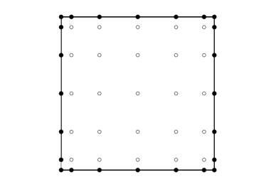
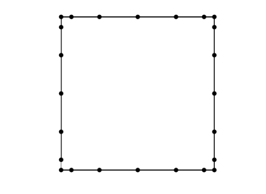
(a)		(b)

Figure 2. Notation for the leaf computation in Section 3. (a) A leaf before elimination of interior (white) nodes. (b) A leaf after elimination of interior nodes.

Let $\bm{\mathsf{w}}\in\mathbb{R}^{p^{2}}$ denote a vector holding the desired approximate solution of (4). We populate all entries corresponding to boundary nodes with the Dirichlet data from $\psi$, and then enforce a spectral collocation condition at the interior nodes. To formalize, let us partition the index set

$$\{1,\,2,\,\dots,\,p^{2}\}=J_{\rm e}\cup J_{\rm i}$$

in such a way that $J_{\rm e}$ contains the $4(p-1)$ nodes on the boundary of $\Omega_{\tau}$, and $J_{\rm i}$ denotes the set of $(p-2)^{2}$ interior nodes, see Figure 2(a). Then partition the vector $\bm{\mathsf{w}}$ into two parts corresponding to internal and exterior nodes via

$$\bm{\mathsf{w}}_{\rm i}=\bm{\mathsf{w}}(J_{\rm i}),\quad\bm{\mathsf{w}}_{\rm e}=\bm{\mathsf{w}}(J_{\rm e}).$$

Analogously, partition $\bm{\mathsf{A}}$ into four parts via

$$\bm{\mathsf{A}}_{\rm i,i}=\bm{\mathsf{A}}(J_{\rm i},J_{\rm i}),\quad\bm{\mathsf{A}}_{\rm i,e}=\bm{\mathsf{A}}(J_{\rm i},J_{\rm e}),\quad\bm{\mathsf{A}}_{\rm e,i}=\bm{\mathsf{A}}(J_{\rm e},J_{\rm i}),\quad\bm{\mathsf{A}}_{\rm e,e}=\bm{\mathsf{A}}(J_{\rm e},J_{\rm e}).$$

The potential at the exterior nodes is now given directly from the boundary condition:

$$\bm{\mathsf{w}}_{\rm e}=\left[\psi(\bm{z}_{k})\right]_{k\in J_{\rm e}}.$$

For the internal nodes, we enforce the PDE (4) via direct collocation:

(6) $$\bm{\mathsf{A}}_{\rm i,i}\,\bm{\mathsf{w}}_{\rm i}+\bm{\mathsf{A}}_{\rm i,e}\,\bm{\mathsf{w}}_{\rm e}=\bm{\mathsf{0}}.$$

Solving (6) for $\bm{\mathsf{w}}_{\rm i}$, we find

(7) $$\bm{\mathsf{w}}_{\rm i}=-\bm{\mathsf{A}}_{\rm i,i}^{-1}\,\bm{\mathsf{A}}_{\rm i,e}\,\bm{\mathsf{w}}_{\rm e},$$

3.2. Constructing the approximate DtN

Now that we know how to approximately solve the local Dirichlet problem (4) via a local spectral method, we can build a matrix $\bm{\mathsf{T}}^{\tau}$ such that (3) holds to high accuracy. The starting point is a vector $\bm{\mathsf{u}}(I_{\tau})\in\mathbb{R}^{4q}$ of tabulated potential values on the boundary of $\Omega_{\tau}$. We will construct the vector $\bm{\mathsf{v}}(I_{\tau})\in\mathbb{R}^{4q}$ via four linear maps. The combination of these maps is the matrix $\bm{\mathsf{T}}^{\tau}$.

Step 1 — re-tabulation from Gaussian nodes to Chebyshev nodes: For each side of $\Omega_{\tau}$, form the unique interpolating polynomial of degree at most $q-1$ that interpolates the $q$ potential values on that side specified by $\bm{\mathsf{u}}(I_{\rm e}^{\tau})$. Now evaluate these polynomials at the boundary nodes of a $p\times p$ Chebyshev grid on $\Omega_{\tau}$. Observe that for a corner node, we may in the general case get conflicts. For instance, the potential at the south-west corner may get one value from extrapolation of potential values on the south border, and one value from extrapolation of the potential values on the west border. We resolve such conflicts by assigning the corner node the average of the two possibly different values. (In practice, essentially no error occurs since we know that the vector $\bm{\mathsf{u}}(I_{\rm e}^{\tau})$ tabulates an underlying function that is continuous at the corner.)

Step 2 — spectral solve: Step 1 populates the boundary nodes of the $p\times p$ Chebyshev grid with Dirichlet data. Now determine the potential at all interior points on the Chebyshev grid by executing a local spectral solve, cf. equation (7).

Step 3 — spectral differentiation: After Step 2, the potential is known at all nodes on the local Chebyshev grid. Now perform spectral differentiation to evaluate approximations to $\partial u/\partial x_{2}$ for the Chebyshev nodes on the two horizontal sides, and $\partial u/\partial x_{1}$ for the Chebyshev nodes on the two vertical sides.

Step 4 — re-tabulation from the Chebyshev nodes back to Gaussian nodes: After Step 3, the boundary fluxes on $\partial\Omega_{\tau}$ are specified by four polynomials of degree $p-1$ (specified via tabulation on the relevant Chebyshev nodes). Now simply evaluate these polynomials at the Gaussian nodes on each side to obtain the vector $\bm{\mathsf{v}}(I_{\rm e}^{\tau})$.

Putting everything together, we find that the matrix $\bm{\mathsf{T}}^{\tau}$ is given as a product of four matrices

$$\begin{array}[]{ccccccccc}\bm{\mathsf{T}}^{\tau}&=&\bm{\mathsf{L}}_{4}&\circ&\bm{\mathsf{L}}_{3}&\circ&\bm{\mathsf{L}}_{2}&\circ&\bm{\mathsf{L}}_{1}\\ 4q\times 4q&&4q\times 4p&&4p\times p^{2}&&p^{2}\times 4(p-1)&&4(p-1)\times 4q\end{array}$$

where $\bm{\mathsf{L}}_{i}$ is the linear transform corresponding to “Step $i$” above. Observe that many of these transforms are far from dense, for instance, $\bm{\mathsf{L}}_{1}$ and $\bm{\mathsf{L}}_{4}$ are $4\times 4$ block matrices with all off-diagonal blocks equal to zero. Exploiting these structures substantially accelerates the computation.

4. Merging two DtN maps

Let $\tau$ denote a box in the tree with children $\alpha$ and $\beta$. In this section, we demonstrate that if the DtN matrices $\bm{\mathsf{T}}^{\alpha}$ and $\bm{\mathsf{T}}^{\beta}$ for the children are known, then the DtN matrix $\bm{\mathsf{T}}^{\tau}$ can be constructed via a purely local computation which we refer to as a “merge” operation.

Figure 3. Notation for the merge operation described in Section 4. The rectangular domain $\Omega$ is formed by two squares $\Omega_{\alpha}$ and $\Omega_{\beta}$. The sets $J_{1}$ and $J_{2}$ form the exterior nodes (black), while $J_{3}$ consists of the interior nodes (white).

We start by introducing some notation: Let $\Omega_{\tau}$ denote a box with children $\Omega_{\alpha}$ and $\Omega_{\beta}$. For concreteness, let us assume that $\Omega_{\alpha}$ and $\Omega_{\beta}$ share a vertical edge as shown in Figure 3, so that

$$\Omega_{\tau}=\Omega_{\alpha}\cup\Omega_{\beta}.$$

We partition the points on $\partial\Omega_{\alpha}$ and $\partial\Omega_{\beta}$ into three sets:

	$J_{1}$	Boundary nodes of $\Omega_{\alpha}$ that are not boundary nodes of $\Omega_{\beta}$.
	$J_{2}$	Boundary nodes of $\Omega_{\beta}$ that are not boundary nodes of $\Omega_{\alpha}$.
	$J_{3}$	Boundary nodes of both $\Omega_{\alpha}$ and $\Omega_{\beta}$ that are not boundary nodes of the union box $\Omega_{\tau}$.

Figure 3 illustrates the definitions of the $J_{k}$’s. Let $u$ denote a solution to (1), with tabulated potential values $\bm{\mathsf{u}}$ and boundary fluxes $\bm{\mathsf{v}}$, as described in Section 2. Set

(8) $$\bm{\mathsf{u}}_{\rm i}=\bm{\mathsf{u}}_{3},\qquad\mbox{and}\qquad\bm{\mathsf{u}}_{\rm e}=\left[\begin{array}[]{c}\bm{\mathsf{u}}_{1}\\ \bm{\mathsf{u}}_{2}\end{array}\right].$$

Recall that $\bm{\mathsf{T}}^{\alpha}$ and $\bm{\mathsf{T}}^{\beta}$ denote the operators that map values of the potential $u$ on the boundary to values of $\partial_{n}u$ on the boundaries of the boxes $\Omega_{\alpha}$ and $\Omega_{\beta}$, as described in Section 3. The operators can be partitioned according to the numbering of nodes in Figure 3, resulting in the equations

(9) $$\left[\begin{array}[]{c}\bm{\mathsf{v}}_{1}\\ \bm{\mathsf{v}}_{3}\end{array}\right]=\left[\begin{array}[]{ccc}\bm{\mathsf{T}}_{1,1}^{\alpha}&\bm{\mathsf{T}}_{1,3}^{\alpha}\\ \bm{\mathsf{T}}_{3,1}^{\alpha}&\bm{\mathsf{T}}_{3,3}^{\alpha}\end{array}\right]\,\left[\begin{array}[]{c}\bm{\mathsf{u}}_{1}\\ \bm{\mathsf{u}}_{3}\end{array}\right],\qquad{\rm and}\qquad\left[\begin{array}[]{c}\bm{\mathsf{v}}_{2}\\ \bm{\mathsf{v}}_{3}\end{array}\right]=\left[\begin{array}[]{ccc}\bm{\mathsf{T}}_{2,2}^{\beta}&\bm{\mathsf{T}}_{2,3}^{\beta}\\ \bm{\mathsf{T}}_{3,2}^{\beta}&\bm{\mathsf{T}}_{3,3}^{\beta}\end{array}\right]\,\left[\begin{array}[]{c}\bm{\mathsf{u}}_{2}\\ \bm{\mathsf{u}}_{3}\end{array}\right].$$

Our objective is now to construct a solution operator $\bm{\mathsf{S}}^{\tau}$ and a DtN matrix $\bm{\mathsf{T}}^{\tau}$ such that

(12) $$\bm{\mathsf{u}}_{3}= \ \bm{\mathsf{S}}^{\tau}\,\left[\begin{array}[]{c}\bm{\mathsf{u}}_{1}\\ \bm{\mathsf{u}}_{2}\end{array}\right]$$

(17) $$\left[\begin{array}[]{c}\bm{\mathsf{v}}_{1}\\ \bm{\mathsf{v}}_{2}\end{array}\right]= \ \bm{\mathsf{T}}^{\tau}\,\left[\begin{array}[]{c}\bm{\mathsf{u}}_{1}\\ \bm{\mathsf{u}}_{2}\end{array}\right].$$

To this end, we eliminate $\bm{\mathsf{v}}_{3}$ from (9) and write the result as a single equation:

(18) $$\left[\begin{array}[]{cc|c}\bm{\mathsf{T}}^{\alpha}_{1,1}&\bm{\mathsf{0}}&\bm{\mathsf{T}}^{\alpha}_{1,3}\\ \bm{\mathsf{0}}&\bm{\mathsf{T}}^{\beta}_{2,2}&\bm{\mathsf{T}}^{\beta}_{2,3}\\ \hline\cr\bm{\mathsf{T}}^{\alpha}_{3,1}&-\bm{\mathsf{T}}^{\beta}_{3,2}&\bm{\mathsf{T}}^{\alpha}_{3,3}-\bm{\mathsf{T}}^{\beta}_{3,3}\end{array}\right]\,\left[\begin{array}[]{c}\bm{\mathsf{u}}_{1}\\ \bm{\mathsf{u}}_{2}\\ \hline\cr\bm{\mathsf{u}}_{3}\end{array}\right]=\left[\begin{array}[]{c}\bm{\mathsf{v}}_{1}\\ \bm{\mathsf{v}}_{2}\\ \hline\cr\bm{\mathsf{0}}\end{array}\right],$$

The last equation directly tells us that (12) holds with

(19) $$\bm{\mathsf{S}}^{\tau}=\bigl{(}\bm{\mathsf{T}}^{\alpha}_{3,3}-\bm{\mathsf{T}}^{\beta}_{3,3}\bigr{)}^{-1}\bigl{[}-\bm{\mathsf{T}}^{\alpha}_{3,1}\ \big{|}\ \bm{\mathsf{T}}^{\beta}_{3,2}].$$

By eliminating $\bm{\mathsf{u}}_{3}$ from (18) by forming a Schur complement, we also find that (17) holds with

(20) $$\bm{\mathsf{T}}^{\tau}=\left[\begin{array}[]{ccc}\bm{\mathsf{T}}_{1,1}^{\alpha}&\bm{\mathsf{0}}\\ \bm{\mathsf{0}}&\bm{\mathsf{T}}_{2,2}^{\beta}\end{array}\right]+\left[\begin{array}[]{c}\bm{\mathsf{T}}_{1,3}^{\alpha}\\ \bm{\mathsf{T}}_{2,3}^{\beta}\end{array}\right]\,\bigl{(}\bm{\mathsf{T}}^{\alpha}_{3,3}-\bm{\mathsf{T}}^{\beta}_{3,3}\bigr{)}^{-1}\bigl{[}-\bm{\mathsf{T}}^{\alpha}_{3,1}\ \big{|}\ \bm{\mathsf{T}}^{\beta}_{3,2}\bigr{]}.$$

5. The full hierarchical scheme

At this point, we know how to construct the DtN operator for a leaf (Section 3), and how to merge two such operators of neighboring patches to form the DtN operator of their union (Section 4). We are ready to describe the full hierarchical scheme for solving the Dirichlet problem (1). This scheme takes the Dirichlet boundary data $f$, and constructs an approximation to the solution $u$. The output is a vector $\bm{\mathsf{u}}$ that tabulates approximations to $u$ at the Gaussian nodes $\{\bm{x}_{k}\}_{k=1}^{N}$ on all interior edges that were defined in Section 2. To find $u$ at an arbitrary set of target points in $\Omega$, a post-processing step described in Section 5.3 can be used.

5.1. The algorithm

Partition the domain into a hierarchical tree as described in Section 2. Then execute a “build stage” in which we construct for each box $\tau$ the following two matrices:

• For a parent box $\tau$, $\bm{\mathsf{S}}^{\tau}$ is a solution operator that maps values of $u$ on $\partial\Omega_{\tau}$ to values of $u$ at the interior nodes. In other words, $\bm{\mathsf{u}}(I_{\rm i}^{\tau})=\bm{\mathsf{S}}^{\tau}\,\bm{\mathsf{u}}(I_{\rm e}^{\tau})$. (For a leaf $\tau$, $\bm{\mathsf{S}}^{\tau}$ is not defined.)

• The matrix that maps $\bm{\mathsf{u}}(I_{\rm e}^{\tau})$ (tabulating values of $u$ on $\partial\Omega_{\tau}$) to $\bm{\mathsf{v}}(I_{\rm e}^{\tau})$ (tabulating values of $du/dn$). In other words, $\bm{\mathsf{v}}(I_{\rm e}^{\tau})=\bm{\mathsf{T}}^{\tau}\,\bm{\mathsf{u}}(I_{\rm e}^{\tau})$.

(Recall that the index vectors $I_{\rm e}^{\tau}$ and $I_{\rm i}^{\tau}$ were defined in Section 2.) The build stage consists of a single sweep over all nodes in the tree. Any bottom-up ordering in which any parent box is processed after its children can be used. For each leaf box $\tau$, an approximation to the local DtN map $\bm{\mathsf{T}}^{\tau}$ is constructed using the procedure described in Section 3. For a parent box $\tau$ with children $\alpha$ and $\beta$, the matrices $\bm{\mathsf{S}}^{\tau}$ and $\bm{\mathsf{T}}^{\tau}$ are formed from the DtN operators $\bm{\mathsf{T}}^{\alpha}$ and $\bm{\mathsf{T}}^{\beta}$ via the process described in Section 4. Algorithm 1 summarizes the build stage.

Once all the matrices $\{\bm{\mathsf{S}}^{\tau}\}_{\tau}$ have been formed, a vector $\bm{\mathsf{u}}$ holding approximations to the solution $u$ of (1) can be constructed for all discretization points by starting at the root box $\Omega$ and moving down the tree toward the leaf boxes. The values of $\bm{\mathsf{u}}$ for the points on the boundary of $\Omega$ can be obtained by tabulating the boundary function $f$. When any box $\tau$ is processed, the value of $\bm{\mathsf{u}}$ is known for all nodes on its boundary (i.e. those listed in $I_{\rm e}^{\tau}$). The matrix $\bm{\mathsf{S}}^{\tau}$ directly maps these values to the values of $\bm{\mathsf{u}}$ on the nodes in the interior of $\tau$ (i.e. those listed in $I_{\rm i}^{\tau}$). When all nodes have been processed, approximations to $u$ have constructed for all tabulation nodes on interior edges. Algorithm 2 summarizes the solve stage.

Algorithm 1 (build solution operators) This algorithm builds the global Dirichlet-to-Neumann operator for (1). It also builds all matrices $\bm{\mathsf{S}}^{\tau}$ required for constructing $u$ at any interior point. It is assumed that if node $\tau$ is a parent of node $\sigma$, then $\tau<\sigma$.   (1) for $\tau=N_{\rm boxes},\,N_{\rm boxes}-1,\,N_{\rm boxes}-2,\,\dots,\,1$ (2) if ($\tau$ is a leaf) (3) Construct $\bm{\mathsf{T}}^{\tau}$ via the process described in Section 3. (4) else (5) Let $\alpha$ and $\beta$ be the children of $\tau$. (6) Split $I_{\rm e}^{\alpha}$ and $I_{\rm e}^{\beta}$ into vectors $I_{1}$, $I_{2}$, and $I_{3}$ as shown in Figure 3. (7) $\bm{\mathsf{S}}^{\tau}=\bigl{(}\bm{\mathsf{T}}^{\alpha}_{3,3}-\bm{\mathsf{T}}^{\beta}_{3,3}\bigr{)}^{-1}\bigl{[}-\bm{\mathsf{T}}^{\alpha}_{3,1}\ \big{|}\ \bm{\mathsf{T}}^{\beta}_{3,2}\bigr{]}$ (8) $\bm{\mathsf{T}}^{\tau}=\left[\begin{array}[]{ccc}\bm{\mathsf{T}}_{1,1}^{\alpha}&\bm{\mathsf{0}}\\ \bm{\mathsf{0}}&\bm{\mathsf{T}}_{2,2}^{\beta}\end{array}\right]+\left[\begin{array}[]{c}\bm{\mathsf{T}}_{1,3}^{\alpha}\\ \bm{\mathsf{T}}_{2,3}^{\beta}\end{array}\right]\,\bm{\mathsf{S}}^{\tau}$. (9) Delete $\bm{\mathsf{T}}^{\alpha}$ and $\bm{\mathsf{T}}^{\beta}$. (10) end if (11) end for

Algorithm 2 (solve BVP once solution operator has been built) This program constructs an approximation $\bm{\mathsf{u}}$ to the solution $u$ of (1). It assumes that all matrices $\bm{\mathsf{S}}^{\tau}$ have already been constructed in a pre-computation. It is assumed that if node $\tau$ is a parent of node $\sigma$, then $\tau<\sigma$.   (1) $\bm{\mathsf{u}}(k)=f(\bm{x}_{k})$ for all $k\in I_{\rm e}^{1}$. (2) for $\tau=1,\,2,\,3,\,\dots,\,N_{\rm boxes}$ (3) if ($\tau$ is a parent) (4) $\bm{\mathsf{u}}(I_{\rm i}^{\tau})=\bm{\mathsf{S}}^{\tau}\,\bm{\mathsf{u}}(I_{\rm e}^{\tau})$. (5) end if (6) end for Remark: This algorithm outputs the solution on the Gaussian nodes on box boundaries. To get the solution at other points, use the method described in Section 5.3.

Remark 3.

The merge stage is exact when performed in exact arithmetic. The only approximation involved is the approximation of the solution $u$ on a leaf by its interpolating polynomial.

Remark 4.

To keep the presentation simple, we consider in this note only the case of a uniform computational grid. Such grids are obviously not well suited to situations where the regularity of the solution changes across the domain. The method described can in principle be modified to handle locally refined grids quite easily. A complication is that the tabulation nodes for two touching boxes will typically not coincide, which requires the introduction of specialized interpolation operators. Efficient refinement strategies also require the development of error indicators that identify the regions where the grid need to be refined. This is work in progress, and will be reported at a later date. We observe that our introduction of Gaussian nodes on the internal boundaries (as opposed to the Chebyshev nodes used in [13]) makes re-interpolation much easier.

5.2. Asymptotic complexity

In this section, we determine the asymptotic complexity of the direct solver. Let $N_{\rm leaf}=4q$ denote the number of Gaussian nodes on the boundary of a leaf box, and let $q^{2}$ denote the number of Chebychev nodes used in the leaf computation. Let $L$ denote the number of levels in the binary tree. This means there are $4^{L}$ boxes. Thus the total number of discretization nodes $N$ is approximately $4^{L}q=\frac{(2^{L}q)^{2}}{q}$. (To be exact, $N=2^{2L+1}q+2^{L+1}q$.)

The cost to process one leaf is approximately $O(q^{6})$. Since there are $\frac{N}{q^{2}}$ leaf boxes, the total cost of pre-computing approximate DtN operators for all the bottom level is $\frac{N}{q^{2}}\times q^{6}\sim Nq^{4}$.

Next, consider the cost of constructing the DtN map on level $\ell$ via the merge operation described in Section 4. For each box on the level $\ell$, the operators $\bm{\mathsf{T}}^{\tau}$ and $\bm{\mathsf{S}}^{\tau}$ are constructed via (19) and (19). These operations involve matrices of size roughly $2^{-\ell}N^{0.5}\times 2^{-\ell}N^{0.5}$. Since there are $4^{\ell}$ boxes per level. The cost on level $\ell$ of the merge is

$$4^{\ell}\times\left(2^{-\ell}N^{0.5}\right)^{3}\sim 2^{-\ell}N^{1.5}.$$

The total cost for all the merge procedures has complexity

$$\sum_{\ell=1}^{L}2^{-\ell}N^{1.5}\sim N^{1.5}.$$

Finally, consider the cost of the downwards sweep which solves for the interior unknowns. For any non-leaf box $\tau$ on level $\ell$, the size of $\bm{\mathsf{S}}^{\tau}$ is $2^{l}q\times 2^{l}(6q)$ which is approximately $\sim 2^{-\ell}N^{0.5}\times 2^{-\ell}N^{0.5}$. Thus the cost of applying $\bm{\mathsf{S}}^{\tau}$ is roughly $(2^{-\ell}N^{0.5})^{2}=2^{-2\ell}N$. So the total cost of the solve step has complexity

$$\sum_{l=0}^{L-1}2^{2\ell}2^{-2\ell}N\sim N\log N.$$

In [6], we explain how to exploit structure in the matrices $\bm{\mathsf{T}}$ and $\bm{\mathsf{S}}$ to improve the computational cost of both the precomputation and the solve steps.

5.3. Post-processing

The direct solver in Algorithm 1 constructs approximations to the solution $u$ of (1) at tabulation nodes at all interior edges. Once these are available, it is easy to construct an approximation to $u$ at an arbitrary point. To illustrate the process, suppose that we seek an approximation to $u(\bm{y})$, where $\bm{y}$ is a point located in a leaf $\tau$. We have values of $u$ tabulated at Gaussian nodes on $\partial\Omega_{\tau}$. These can easily be re-interpolated to the Chebyshev nodes on $\partial\Omega_{\tau}$. Then $u$ can be reconstructed at the interior Chebyshev nodes via the formula (7); observe that the local solution operator $-\bm{\mathsf{A}}_{\rm i,i}^{-1}\bm{\mathsf{A}}_{\rm i,e}$ was built when the leaf was originally processed and can be simply retrieved from memory (assuming enough memory is available). Once $u$ is tabulated at the Chebyshev grid on $\Omega_{\tau}$, it is trivial to interpolate it to $\bm{y}$ or any other point.

6. Body loads

Now that we have described how to solve our basic boundary value problem

(21) $$\left\{\begin{aligned} \mbox{}[Au](\bm{x})=&\ g(\bm{x}),\qquad&\bm{x}\in\Omega,\\ u(\bm{x})=&\ f(\bm{x}),\qquad&\bm{x}\in\Gamma,\end{aligned}\right.$$

for the special case where $g=0$, we will next consider the more general case that includes a body load. Only minor modifications are required to the basic scheme, but note that the resulting method requires substantially more memory. The techniques presented here were developed jointly with Tracy Babb of CU-Boulder, cf. [10].

6.1. Notation

When handling body loads, we will extensively switch between the Chebyshev and Gaussian grids, so we need to introduce some additional notation.

Let $\{\bm{y}_{j}\}_{j=1}^{M}$ denote the global grid obtained by putting down a $p\times p$ tensor product grid of Chebyshev nodes on each leaf. For a leaf $\tau$, let $I_{\rm c}^{\tau}$ denote an index vector pointing to the nodes in $\{\bm{y}_{j}\}_{j=1}^{M}$ that lie on leaf $\tau$. We partition this index vector into exterior and interior nodes as follows

$$I_{\rm c}^{\tau}=I_{\rm ce}^{\tau}\cup I_{\rm ci}^{\tau}.$$

To avoid confusion with the index vectors pointing into the grid of Gaussian boundary functions, we rename these index vectors as follows:

$I_{\rm ge}^{\tau}$:

An index vector marking the (Gauss) nodes in $\{\bm{x}_{i}\}_{i=1}^{N}$ that lie on $\partial\Omega_{\tau}$.

$I_{\rm gi}^{\tau}$:

For a parent node $\tau$, this is an index vector marking the (Gauss) nodes in $\{\bm{x}_{i}\}_{i=1}^{N}$ that lie on the “interior” boundary of $\tau$. For a leaf node, this vector is not defined.

The fact that we use two spectral grids also leads to a need to distinguish between different vectors tabulating approximate values. We have:

	$\tau$ is a leaf	$\tau$ is a parent
$\bm{\mathsf{u}}_{\rm c}^{\tau}$	$u$ tabulated on Chebyshev nodes	—
$\bm{\mathsf{u}}_{\rm ce}^{\tau}$	$u$ tabulated on Chebyshev exterior nodes	—
$\bm{\mathsf{u}}_{\rm ci}^{\tau}$	$u$ tabulated on Chebyshev interior nodes	—
$\bm{\mathsf{u}}_{\rm ge}^{\tau}$	$u$ tabulated on Gaussian exterior nodes	$u$ tabulated on Gaussian exterior nodes
$\bm{\mathsf{u}}_{\rm gi}^{\tau}$	—	$u$ tabulated on Gaussian interior nodes

6.2. Leaf computation

Let $\tau$ be a leaf. We split the solution $u$ to the equation

(22) $$\left\{\begin{aligned} Au(\bm{x})=&\ g(\bm{x}),\qquad&\bm{x}\in\Omega_{\tau},\\ u(\bm{x})=&\ \psi(\bm{x}),\qquad&\bm{x}\in\Gamma_{\tau},\end{aligned}\right.$$

as

$$u=w+\phi$$

where $w$ is a particular solution

(23) $$\left\{\begin{aligned} Aw(\bm{x})=&\ g(\bm{x}),\qquad&\bm{x}\in\Omega_{\tau},\\ w(\bm{x})=&\ 0,\qquad&\bm{x}\in\Gamma_{\tau},\end{aligned}\right.$$

and where $\phi$ is a homogeneous solution

(24) $$\left\{\begin{aligned} A\phi(\bm{x})=&\ 0,\qquad&\bm{x}\in\Omega_{\tau},\\ \phi(\bm{x})=&\ \psi(\bm{x}),\qquad&\bm{x}\in\Gamma_{\tau}.\end{aligned}\right.$$

We can now write the Neumann data for $u$ as

$$\partial_{n}u|_{\Gamma_{\tau}}=\partial_{n}w|_{\Gamma_{\tau}}+\partial_{n}\phi|_{\Gamma_{\tau}}=\partial_{n}w|_{\Gamma_{\tau}}+T\phi|_{\Gamma_{\tau}}=\partial_{n}w|_{\Gamma_{\tau}}+T\,\psi,$$

where, as before, $T$ is the NfD operator. Our objective is therefore to find a matrix that maps the given body load $g$ on $\Omega_{\tau}$ to the Neumann data of $w$. We do this calculation on the Chebyshev grid. Discretizing (23), and collocating on the internal nodes, we find

$$\bm{\mathsf{A}}_{\rm ci,ce}\bm{\mathsf{w}}_{\rm ce}+\bm{\mathsf{A}}_{\rm ci,ci}\bm{\mathsf{w}}_{\rm ci}=\bm{\mathsf{g}}_{\rm ci}.$$

But now observe that $\bm{\mathsf{w}}_{\rm ce}=0$, so the particular solution is given by

$$\bm{\mathsf{w}}_{\rm c}=\left[\begin{array}[]{c}\bm{\mathsf{w}}_{\rm ce}\\ \bm{\mathsf{w}}_{\rm ci}\end{array}\right]=\bm{\mathsf{F}}_{\rm c,ci}\bm{\mathsf{g}}_{\rm ci},\qquad\mbox{where}\qquad\bm{\mathsf{F}}_{\rm c,ci}=\left[\begin{array}[]{c}\bm{\mathsf{0}}\\ \bm{\mathsf{A}}_{\rm ci,ci}^{-1}\end{array}\right].$$

Let $\bm{\mathsf{h}}_{\rm ge}$ denote the Neumann data for $\bm{\mathsf{w}}$, tabulated at the Gaussian nodes on the boundary. It follows that

$$\bm{\mathsf{h}}_{\rm ge}=\underbrace{\bm{\mathsf{D}}_{\rm ge,c}\bm{\mathsf{F}}_{\rm c,ci}}_{=:\bm{\mathsf{H}}_{\rm ge,ci}}\bm{\mathsf{g}}_{\rm ci},$$

where $\bm{\mathsf{D}}_{\rm ge,c}$ is the operator that differentiates from the full Chebyshev grid, and then interpolates to the Gaussian exterior nodes. (Using the notation from Section 4, $\bm{\mathsf{D}}_{\rm ge,c}=\bm{\mathsf{L}}_{4}\bm{\mathsf{L}}_{3}$.)

Once the boundary data of $u$ on $\Omega_{\tau}$ is given, the total solution on the Chebyshev grid is given by

$$\bm{\mathsf{u}}_{\rm c}=\bm{\mathsf{S}}_{\rm c,ge}\bm{\mathsf{u}}_{\rm ge}+\bm{\mathsf{F}}_{\rm c,ci}\bm{\mathsf{g}}_{\rm ci}=\bm{\mathsf{S}}_{\rm c,ge}\bm{\mathsf{u}}_{\rm ge}+\bm{\mathsf{w}}_{\rm c},$$

where $\bm{\mathsf{S}}_{\rm c,ge}$ is the solution operator given by

$$\bm{\mathsf{S}}_{\rm c,ge}=\left[\begin{array}[]{c}\bm{\mathsf{I}}\\ -\bm{\mathsf{A}}_{\rm ci,ci}^{-1}\bm{\mathsf{A}}_{\rm ci,ce}\end{array}\right]\bm{\mathsf{I}}_{\rm ce,ge},$$

where, in turn, $\bm{\mathsf{I}}_{\rm ce,ge}$ is the interpolation operator that maps from the boundary Gauss nodes to the boundary Chebyshev nodes.

6.3. Merge operator

Let $\tau$ be a parent node with children $\alpha$ and $\beta$. The local equilibrium equations read

(33) $$\left[\begin{array}[]{c}\bm{\mathsf{v}}_{1}\\ \bm{\mathsf{v}}_{3}\end{array}\right]= \ \left[\begin{array}[]{ccc}\bm{\mathsf{T}}_{1,1}^{\alpha}&\bm{\mathsf{T}}_{1,3}^{\alpha}\\ \bm{\mathsf{T}}_{3,1}^{\alpha}&\bm{\mathsf{T}}_{3,3}^{\alpha}\end{array}\right]\,\left[\begin{array}[]{c}\bm{\mathsf{u}}_{1}\\ \bm{\mathsf{u}}_{3}\end{array}\right]+\left[\begin{array}[]{c}\bm{\mathsf{h}}_{1}^{\alpha}\\ \bm{\mathsf{h}}_{3}^{\alpha}\end{array}\right],$$

(42) $$\left[\begin{array}[]{c}\bm{\mathsf{v}}_{2}\\ \bm{\mathsf{v}}_{3}\end{array}\right]= \ \left[\begin{array}[]{ccc}\bm{\mathsf{T}}_{2,2}^{\beta}&\bm{\mathsf{T}}_{2,3}^{\beta}\\ \bm{\mathsf{T}}_{3,2}^{\beta}&\bm{\mathsf{T}}_{3,3}^{\beta}\end{array}\right]\,\left[\begin{array}[]{c}\bm{\mathsf{u}}_{2}\\ \bm{\mathsf{u}}_{3}\end{array}\right]+\left[\begin{array}[]{c}\bm{\mathsf{h}}_{2}^{\beta}\\ \bm{\mathsf{h}}_{3}^{\beta}\end{array}\right].$$

Combine the two equations for $\bm{\mathsf{v}}_{3}$ to obtain the equation

$$\bm{\mathsf{T}}_{3,1}^{\alpha}\,\bm{\mathsf{u}}_{1}+\bm{\mathsf{T}}_{3,3}^{\alpha}\,\bm{\mathsf{u}}_{3}+\bm{\mathsf{h}}_{3}^{\alpha}=\bm{\mathsf{T}}_{3,2}^{\beta}\,\bm{\mathsf{u}}_{2}+\bm{\mathsf{T}}_{3,3}^{\beta}\,\bm{\mathsf{u}}_{3}+\bm{\mathsf{h}}_{3}^{\beta}.$$

This gives [check for sign errors!]

(43) $$\bm{\mathsf{u}}_{3}=\bigl{(}\bm{\mathsf{T}}^{\alpha}_{3,3}-\bm{\mathsf{T}}^{\beta}_{3,3}\bigr{)}^{-1}\bigl{(}\bm{\mathsf{T}}^{\beta}_{3,2}\bm{\mathsf{u}}_{2}-\bm{\mathsf{T}}^{\alpha}_{3,1}\bm{\mathsf{u}}_{1}+\bm{\mathsf{h}}_{3}^{\beta}-\bm{\mathsf{h}}_{3}^{\alpha}\bigr{)}$$

Inserting (43) back into (33) we find

$$\left[\begin{array}[]{c}\bm{\mathsf{v}}_{1}\\ \bm{\mathsf{v}}_{2}\end{array}\right]= \ \left(\left[\begin{array}[]{ccc}\bm{\mathsf{T}}_{1,1}^{\alpha}&\bm{\mathsf{0}}\\ \bm{\mathsf{0}}&\bm{\mathsf{T}}_{2,2}^{\beta}\end{array}\right]+\left[\begin{array}[]{c}\bm{\mathsf{T}}_{1,3}^{\alpha}\\ \bm{\mathsf{T}}_{2,3}^{\beta}\end{array}\right]\,\bigl{(}\bm{\mathsf{T}}^{\alpha}_{3,3}-\bm{\mathsf{T}}^{\beta}_{3,3}\bigr{)}^{-1}\bigl{[}-\bm{\mathsf{T}}^{\alpha}_{3,1}\ \big{|}\ \bm{\mathsf{T}}^{\beta}_{3,2}].\right)\left[\begin{array}[]{c}\bm{\mathsf{u}}_{1}\\ \bm{\mathsf{u}}_{2}\end{array}\right]+$$

$$\ \left[\begin{array}[]{c}\bm{\mathsf{h}}^{\alpha}_{1}\\ \bm{\mathsf{h}}^{\beta}_{2}\end{array}\right]+\left[\begin{array}[]{c}\bm{\mathsf{T}}_{1,3}^{\alpha}\\ \bm{\mathsf{T}}_{2,3}^{\beta}\end{array}\right]\,\bigl{(}\bm{\mathsf{T}}^{\alpha}_{3,3}-\bm{\mathsf{T}}^{\beta}_{3,3}\bigr{)}^{-1}\bigl{(}\bm{\mathsf{h}}_{3}^{\beta}-\bm{\mathsf{h}}_{3}^{\alpha}\bigr{)}.$$

We now define operators

$$\bm{\mathsf{X}}^{\tau}_{\rm gi,gi}= \ \bigl{(}\bm{\mathsf{T}}^{\alpha}_{3,3}-\bm{\mathsf{T}}^{\beta}_{3,3}\bigr{)}^{-1},$$

$$\bm{\mathsf{S}}^{\tau}_{\rm gi,ge}= \ \bigl{(}\bm{\mathsf{T}}^{\alpha}_{3,3}-\bm{\mathsf{T}}^{\beta}_{3,3}\bigr{)}^{-1}\bigl{[}-\bm{\mathsf{T}}^{\alpha}_{3,1}\ \big{|}\ \bm{\mathsf{T}}^{\beta}_{3,2}]=\bm{\mathsf{X}}^{\tau}_{\rm gi,gi}\bigl{[}-\bm{\mathsf{T}}^{\alpha}_{3,1}\ \big{|}\ \bm{\mathsf{T}}^{\beta}_{3,2}],$$

$$\bm{\mathsf{T}}^{\tau}_{\rm ge,ge}= \left[\begin{array}[]{ccc}\bm{\mathsf{T}}_{1,1}^{\alpha}&\bm{\mathsf{0}}\\ \bm{\mathsf{0}}&\bm{\mathsf{T}}_{2,2}^{\beta}\end{array}\right]\bigl{(}\bm{\mathsf{T}}^{\alpha}_{3,3}-\bm{\mathsf{T}}^{\beta}_{3,3}\bigr{)}^{-1}\bigl{[}-\bm{\mathsf{T}}^{\alpha}_{3,1}\ \big{|}\ \bm{\mathsf{T}}^{\beta}_{3,2}]=\left[\begin{array}[]{ccc}\bm{\mathsf{T}}_{1,1}^{\alpha}&\bm{\mathsf{0}}\\ \bm{\mathsf{0}}&\bm{\mathsf{T}}_{2,2}^{\beta}\end{array}\right]\bm{\mathsf{S}}^{\tau}_{\rm gi,ge}.$$

Then in the upwards pass in the solve, we compute

$$\bm{\mathsf{w}}_{\rm gi}^{\tau}= \ \bm{\mathsf{X}}^{\tau}\bigl{(}\bm{\mathsf{h}}_{3}^{\beta}-\bm{\mathsf{h}}_{3}^{\alpha}\bigr{)}$$

$$\bm{\mathsf{h}}_{\rm ge}^{\tau}= \ \left[\begin{array}[]{c}\bm{\mathsf{T}}_{1,3}^{\alpha}\\ \bm{\mathsf{T}}_{2,3}^{\beta}\end{array}\right]\bm{\mathsf{w}}_{\rm gi}^{\tau},$$

and in the solve stage, we recover $\bm{\mathsf{u}}_{\rm gi}^{\tau}$ via

$$\bm{\mathsf{u}}^{\tau}_{\rm gi}=\bm{\mathsf{S}}_{\rm gi,ge}\bm{\mathsf{u}}^{\tau}_{\rm ge}+\bm{\mathsf{w}}_{\rm gi}^{\tau}.$$

Remark 5 (Physical interpretation of merge).

The quantities $\bm{\mathsf{w}}^{\tau}_{\rm gi}$ and $\bm{\mathsf{h}}_{\rm ge}^{\tau}$ have a simple physical meaning. The vector $\bm{\mathsf{w}}_{\rm gi}^{\tau}$ introduced above is simply a tabulation of the particular solution $w^{\tau}$ associated with $\tau$ on the interior boundary $\Gamma_{3}$, and $\bm{\mathsf{h}}_{\rm ge}^{\tau}$ is the normal derivative of $w^{\tau}$. To be precise, $w^{\tau}$ is the solution to the inhomogeneous problem, cf. (23)

(44) $$\left\{\begin{aligned} Aw^{\tau}(\bm{x})=&\ g(\bm{x}),\qquad&\bm{x}\in\Omega_{\tau},\\ w^{\tau}(\bm{x})=&\ 0,\qquad&\bm{x}\in\Gamma_{\tau}.\end{aligned}\right.$$

We can re-derive the formula for $w|_{\Gamma_{3}}$ using the original mathematical operators as follows: First observe that for $\bm{x}\in\Omega^{\alpha}$, we have $A(w^{\tau}-w^{\alpha})=g-g=0$, so the NfD operator $T^{\alpha}$ applies to the function $w^{\tau}-w^{\alpha}$:

$$T^{\alpha}_{31}(w_{1}^{\tau}-w_{1}^{\alpha})+T^{\alpha}_{33}(w_{3}^{\tau}-w_{3}^{\alpha})=(\partial_{n}w^{\tau})|_{3}-(\partial_{n}w^{\alpha})|_{3}$$

Use that $w_{1}^{\tau}=w_{1}^{\alpha}=w_{3}^{\alpha}=0$, and that $(\partial_{n}w^{\alpha})|_{3}=h_{3}^{\alpha}$ to get

(45) $$T^{\alpha}_{33}w_{3}^{\tau}=(\partial_{n}w^{\tau})|_{3}-h_{3}^{\alpha}.$$

Analogously, we get

(46) $$T^{\beta}_{33}w_{3}^{\tau}=(\partial_{n}w^{\tau})|_{3}-h_{3}^{\beta}.$$

Combine (45) and (46) to eliminate $(\partial_{n}w^{\tau})|_{3}$ and obtain

$$\bigl{(}T^{\alpha}_{33}-T^{\beta}_{33}\bigr{)}w_{3}^{\tau}=-h_{3}^{\alpha}+h_{3}^{\beta}.$$

Observe that in effect, we can write the particular solution $w^{\tau}$ as

$$w^{\tau}(\bm{x})=\left\{\begin{array}[]{ll}w^{\alpha}(\bm{x})+\hat{w}^{\tau}(\bm{x})&\bm{x}\in\Omega^{\alpha},\\ w^{\beta}(\bm{x})+\hat{w}^{\tau}(\bm{x})&\bm{x}\in\Omega^{\beta},\end{array}\right.$$

The function $w^{\tau}$ must of course be smooth across $\Gamma_{3}$, so the function $\hat{w}^{\tau}$ must have a jump that exactly offsets the discrepancy in the derivatives of $w^{\alpha}$ and $w^{\beta}$. This jump is precisely of size $h^{\alpha}-h^{\beta}$.

Algorithm 3 (Build stage for problems with body load) This algorithms build all solution operators required to solve the non-homogeneous BVP (22). It is assumed that if node $\tau$ is a parent of node $\sigma$, then $\tau<\sigma$.   for $\tau=N_{\rm boxes},\,N_{\rm boxes}-1,\,N_{\rm boxes}-2,\,\dots,\,1$ if ($\tau$ is a leaf) $\bm{\mathsf{F}}_{\rm c,ci}^{\tau}=\left[\begin{array}[]{c}\bm{\mathsf{0}}\\ \bm{\mathsf{A}}_{\rm ci,ci}^{-1}\end{array}\right]$  [pot.] $\leftarrow$ [body load] $\bm{\mathsf{H}}_{\rm ge,ci}^{\tau}=\bm{\mathsf{D}}_{\rm ge,c}\bm{\mathsf{F}}_{\rm c,ci}^{\tau}$  [deriv.] $\leftarrow$ [body load] $\bm{\mathsf{S}}_{\rm c,ge}^{\tau}=\left[\begin{array}[]{c}\bm{\mathsf{I}}\\ -\bm{\mathsf{A}}_{\rm ci,ci}^{-1}\bm{\mathsf{A}}_{\rm ci,ce}\end{array}\right]\,\bm{\mathsf{I}}_{\rm ce,ge}$  [pot.] $\leftarrow$ [pot.] $\bm{\mathsf{T}}_{\rm ge,ge}^{\tau}=\bm{\mathsf{D}}_{\rm ge,c}\bm{\mathsf{S}}_{\rm c,ge}$  [deriv.] $\leftarrow$ [pot.] (NfD operator) else Let $\alpha$ and $\beta$ be the children of $\tau$. Partition $I_{\rm e}^{\alpha}$ and $I_{\rm e}^{\beta}$ into vectors $I_{1}$, $I_{2}$, and $I_{3}$ as shown in Figure 3. $\bm{\mathsf{X}}_{\rm gi,gi}^{\tau}=\bigl{(}\bm{\mathsf{T}}^{\alpha}_{3,3}-\bm{\mathsf{T}}^{\beta}_{3,3}\bigr{)}^{-1}$  [pot.] $\leftarrow$ [deriv.] $\bm{\mathsf{S}}_{\rm gi,ge}^{\tau}=\bm{\mathsf{X}}_{\rm gi,gi}^{\tau}\bigl{[}-\bm{\mathsf{T}}^{\alpha}_{3,1}\ \big{|}\ \bm{\mathsf{T}}^{\beta}_{3,2}\bigr{]}$  [pot.] $\leftarrow$ [pot.] $\bm{\mathsf{T}}_{\rm ge,ge}^{\tau}=\left[\begin{array}[]{ccc}\bm{\mathsf{T}}_{1,1}^{\alpha}&\bm{\mathsf{0}}\\ \bm{\mathsf{0}}&\bm{\mathsf{T}}_{2,2}^{\beta}\end{array}\right]+\left[\begin{array}[]{c}\bm{\mathsf{T}}_{1,3}^{\alpha}\\ \bm{\mathsf{T}}_{2,3}^{\beta}\end{array}\right]\,\bm{\mathsf{U}}_{\rm gi,ge}^{\tau}$  [deriv.] $\leftarrow$ [pot.] (NfD operator). end if end for

Figure 4. Build stage.

Algorithm 4 (Solver for problems with body load) This program constructs an approximation $\bm{\mathsf{u}}$ to the solution $u$ of (1). It assumes that all matrices required to represent the solution operator have already been constructed using Algorithm 3. It is assumed that if node $\tau$ is a parent of node $\sigma$, then $\tau<\sigma$.   Upwards pass — construct all particular solutions: for $\tau=N_{\rm boxes},\,N_{\rm boxes}-1,\,N_{\rm boxes}-2,\,\dots,\,1$ if ($\tau$ is a leaf) # Compute the derivatives of the local particular solution. $\bm{\mathsf{h}}_{\rm ge}^{\tau}=\bm{\mathsf{H}}_{\rm ge,ci}^{\tau}\,\bm{\mathsf{g}}_{\rm ci}^{\tau}$ else Let $\alpha$ and $\beta$ denote the children of $\tau$. # Compute the local particular solution. $\bm{\mathsf{w}}_{\rm gi}^{\tau}=\bm{\mathsf{X}}_{\rm gi,gi}^{\tau}\,\bigl{(}-\bm{\mathsf{h}}_{3}^{\alpha}+\bm{\mathsf{h}}_{3}^{\beta}\bigr{)}.$ # Compute the derivatives of the local particular solution. $\bm{\mathsf{h}}_{\rm ge}^{\tau}=\left[\begin{array}[]{c}\bm{\mathsf{h}}_{1}^{\alpha}\\ \bm{\mathsf{h}}_{2}^{\beta}\end{array}\right]+\left[\begin{array}[]{c}\bm{\mathsf{T}}_{1,3}^{\alpha}\\ \bm{\mathsf{T}}_{2,3}^{\beta}\end{array}\right]\,\bm{\mathsf{w}}_{\rm gi}^{\tau}.$ end if end for Downwards pass — construct all potentials: # Use the provided Dirichlet data to set the solution on the exterior of the root. $\bm{\mathsf{u}}(k)=f(\bm{x}_{k})$ for all $k\in I_{\rm e}^{1}$. for $\tau=1,\,2,\,3,\,\dots,\,N_{\rm boxes}$ if ($\tau$ is a parent) # Add the homogeneous term and the particular term. $\bm{\mathsf{u}}_{\rm gi}^{\tau}=\bm{\mathsf{U}}_{\rm gi,ge}^{\tau}\,\bm{\mathsf{u}}_{\rm ge}^{\tau}+\bm{\mathsf{w}}_{\rm gi}^{\tau}$. else # Add the homogeneous term and the particular term. $\bm{\mathsf{u}}_{\rm c}^{\tau}=\bm{\mathsf{U}}_{\rm c,ge}^{\tau}\,\bm{\mathsf{u}}_{\rm ge}^{\tau}+\bm{\mathsf{F}}_{\rm c,ci}^{\tau}\,\bm{\mathsf{g}}_{\rm ci}^{\tau}$. end end for

Figure 5. Solve stage.

Appendix A A graphical illustration of the algorithm

This section provides an illustrated overview of the hierarchical merge process described in detail in Section 5.1. The figures illustrate a situation in which a square domain $\Omega=[0,1]^{2}$ is split into $4\times 4$ leaf boxes on the finest level, and a $6\times 6$ spectral grid is used in each leaf.

Step 1: Partition the box $\Omega$ into $16$ small boxes that each holds an $6\times 6$ Cartesian mesh of Chebyshev nodes. For each box, identify the internal nodes (marked in blue) and eliminate them as described in Section 3. Construct the solution operator $\bm{\mathsf{U}}$, and the DtN operators encoded in the matrices $\bm{\mathsf{V}}$ and $\bm{\mathsf{W}}$.

Step 2: Switch tabulation points on the boundary from Chebyshev nodes to Legendre nodes. The main purpose is to remove the corner nodes.

Step 3: Merge the small boxes by pairs as described in Section 4. The equilibrium equation for each rectangle is formed using the DtN operators of the two small squares it is made up of. The result is to eliminate the interior nodes (marked in blue) of the newly formed larger boxes. Construct the solution operator $\bm{\mathsf{U}}$ and the DtN matrices $\bm{\mathsf{V}}$ and $\bm{\mathsf{W}}$ for the new boxes.

Step 4: Merge the boxes created in Step 3 in pairs, again via the process described in Section 4.

Step 5: Repeat the merge process once more.

Step 6: Repeat the merge process one final time to obtain the DtN operator for the boundary of the whole domain.

References

• [1] Mario Bebendorf, Hierarchical matrices, Lecture Notes in Computational Science and Engineering, vol.Β 63, Springer-Verlag, Berlin, 2008, A means to efficiently solve elliptic boundary value problems. MR 2451321 (2009k:15001)
• [2] Steffen BΓΆrm, Efficient numerical methods for non-local operators, EMS Tracts in Mathematics, vol.Β 14, European Mathematical Society (EMS), ZΓΌrich, 2010, ${\mathcal{H}}{{}^{2}}$-matrix compression, algorithms and analysis. MR 2767920
• [3] TimothyΒ A Davis, Direct methods for sparse linear systems, vol.Β 2, Siam, 2006.
• [4] I.S. Duff, A.M. Erisman, and J.K. Reid, Direct methods for sparse matrices, Oxford, 1989.
• [5] A.Β George, Nested dissection of a regular finite element mesh, SIAM J. on Numerical Analysis 10 (1973), 345–363.
• [6] A.Β Gillman and P.Β Martinsson, A direct solver with $o(n)$ complexity for variable coefficient elliptic pdes discretized via a high-order composite spectral collocation method, SIAM Journal on Scientific Computing 36 (2014), no.Β 4, A2023–A2046, arXiv.org report #1307.2665.
• [7] Adrianna Gillman, AlexH. Barnett, and Per-Gunnar Martinsson, A spectrally accurate direct solution technique for frequency-domain scattering problems with variable media, BIT Numerical Mathematics 55 (2015), no.Β 1, 141–170 (English).
• [8] W.Β Hackbusch, B.Β Khoromskij, and S.Β Sauter, On $\mathcal{H}^{2}$-matrices, Lectures on Applied Mathematics, Springer Berlin, 2002, pp.Β 9–29.
• [9] Wolfgang Hackbusch, A sparse matrix arithmetic based on H-matrices; Part I: Introduction to H-matrices, Computing 62 (1999), 89–108.
• [10] T.S. Haut, T.Β Babb, P.G. Martinsson, and B.A. Wingate, A high-order scheme for solving wave propagation problems via the direct construction of an approximate time-evolution operator, arXiv preprint arXiv:1402.5168 (2014).
• [11] J.S. Hesthaven, P.G. Dinesen, and J.P. Lynov, Spectral collocation time-domain modeling of diffractive optical elements, Journal of Computational Physics 155 (1999), no.Β 2, 287 – 306.
• [12] P.G. Martinsson, A composite spectral scheme for variable coefficient helmholtz problems, arXiv preprint arXiv:1206.4136 (2012).
• [13] P.G. Martinsson, A direct solver for variable coefficient elliptic pdes discretized via a composite spectral collocation method, Journal of Computational Physics 242 (2013), no.Β 0, 460 – 479.
• [14] H.P. Pfeiffer, L.E. Kidder, M.A. Scheel, and S.A. Teukolsky, A multidomain spectral method for solving elliptic equations, Computer physics communications 152 (2003), no.Β 3, 253–273.
• [15] L.N. Trefethen, Spectral methods in matlab, SIAM, Philadelphia, 2000.