On some aspects of the discretization of the Suslov problem

Abstract.

In this paper we explore the discretization of Euler-Poincaré-Suslov equations on $SO(3)$, i.e. of the Suslov problem. We show that the consistency order corresponding to the unreduced and reduced setups, when the discrete reconstruction equation is given by a Cayley retraction map, are related to each other in a nontrivial way. We give precise conditions under which general and variational integrators generate a discrete flow preserving the constraint distribution. We establish general consistency bounds and illustrate the performance of several discretizations by some plots. Moreover, along the lines of [15] we show that any constraints-preserving discretization may be understood as being generated by the exact evolution map of a time-periodic non-autonomous perturbation of the original continuous-time nonholonomic system.

1. Introduction

The Lagrangian formulation of mechanical systems with nonholonomic constraints has been extensively studied in recent years (see [3, 19] for a complete description and extensive bibliographies). In short, this kind of systems are characterized by so-called nonholonomic constraints, i.e. constraints involving both configuration as well as velocity variables, and which can not be integrated to purely configuration-dependent constraints (in this case the constraints are called holonomic). Moreover, the preservation of certain structural properties of mechanical systems by suitable integrators is a delicate issue upon which a lot of attention has been put by the Geometric Mechanics comunity (see the recent works, such as [8, 11, 12, 16, 17, 23], which have introduced numerical integrators for holonomic systems with very good energy behavior and various preservation properties). The approaches in most of these references are based on the ideas of [22, 24]. In these works, the continuous variational principles are replaced by discrete ones aiming to obtain proper integrators approximating the continuous dynamics. We will call the integrators related to this framework variational integrators. Analogously, in the case of nonholonomic mechanics, the continuous Lagrange-d’Alembert’s principle, which provides the actual dynamics, is replaced by a discrete Lagrange-d’Alembert’s principle on the discrete phase space. Of special interest are the seminal works on nonholonomic integration [8, 23], where a discrete version of the Lagrange-d’Alembert principle is proposed by introducing a proper discretization of the nonholonomic distribution. In [15], the focus has been on numerical integrators including variational integrators that exactly respect the original continuous constraint distribution. Also, corresponding consistency estimates were derived. In particular, it has been shown that any integrator that preserves the original continuous constraint distribution may be understood as being generated by the exact evolution map of a time-periodic non-autonomous perturbation of the continuous-time nonholonomic system, where the size of the perturbation is related to the order of consistency of the integrator.

Reduction theory is one of the fundamental tools in the study of mechanical systems with symmetry and it concerns the removal of symmetries using the associated conservation laws. A Lagrangian system is called symmetric w.r.t. a Lie group if the Lagrangian function is invariant under the tangent lift of the action of the Lie group on the configuration manifold. Furthermore, for a symmetric mechanical system the process of reduction eliminates the directions along the group variables and thus provides a system with fewer degrees of freedom. When the configuration manifold is the Lie group itself, for unconstrained Lagrangian systems the process of reduction leads from the Euler-Lagrange equations to the Euler-Poincaré equations. Needless to say, nonholonomic systems may also possess symmetries, and the geometrical treatment of such situations has been studied in [4, 7] among other references. On the other hand, variational integrators for reduced systems were carefully studied from the theoretical point of view in [20, 21]. The combination of these two issues, i.e. variational integrators in the context of symmetric nonholonomic Lagrangian systems, has been addressed in [10] in the case of a ll system, i.e. a nonholonomic system whose configuration manifold is a Lie group $G$, and where both the Lagrangian and the constraint distribution are invariant with respect to the induced left action of $G$ on $TG$. Here,the dynamics of the reduced system is described by the Euler-Poincaré-Suslov equations [18, 25]. Other interesting discretizations of symmetric nonholonomic systems can be found in [9].

The Euler-Poincaré-Suslov equations on $SO(3)$, i.e. the Suslov problem [25], are the object of study in the present paper, more concretely from the point of view of the results presented in [15]. Particularly, we focus on their discretization and meticulously study conditions under which the constraints are preserved by the corresponding integrator. Both, general as wll as variational intgrators will be considered. We study the relationship between the orders of consistency of integrators in the unreduced and reduced setting, that are related by reconstruction and reduction, respectively. We find out that the relationship is nontrivial, and we figure it out precisely for the case of a particular retraction map relating $SO(3)$ and $\mathfrak{so}(3)$, namely the Cayley map. The study of consistency requires the introduction of a suitable metric on $SO(3)$. We present numerical results for several integrators and carefully study their order of consistency. Finally, we address the issue of discrepancies between the continuous and the discrete dynamics for the Suslov problem based on previous results in [13, 15].

The paper is structured as follows: In §2, §3 and §4 we provide a comprehensive introduction to nonholonomic mechanics, variational nonholonomic integrators, symmetries of nonholonomic Lagrangian systems, the Euler-Poincaré-Suslov equations and, finally, variational integrators for reduced systems. We provide a new version of the discrete Euler-Poincaré-Suslov equations, defined on the Lie algebra through the incorporation of a retraction map, in corollary 4.4. §5 establishes the link between the results in [15] and the reduced framework for $SO(3)$, i.e. we perform an exhaustive study of the Suslov problem. First, §5.3 is devoted to the study of consistency orders as mentioned above. Then, in subsection §5.4, we study general discretizations, as well as sufficient conditions in the case of variational integrators that guarantee preservationof the continuous-time constraint distribution. In §5.5, we give consistency results both for general and variational discretizations, and illustrate their performance through some plots. Finally, §6 is devoted to the study of distribution-preserving discretizations of the Euler-Poincaré-Suslov problem viewed as perturbation of the continuous dynamics. Here, we apply the result by Fiedler and Scheurle [13] to the system under consideration, and establish a bound of the perturbation produced in the unreduced dynamics by a reduced integrator, and conversely.

Throughout the paper, we use Einstein’s convention for the summation over repeated indices unless the opposite is stated.

2. Preliminaries

2.1. The nonholonomic setting

We define a nonholonomic Lagrangian system on a Lie group as a triple $(G,L,D)$, where $G$ is the Lie group, $L:TG\rightarrow\mathds{R}$ is the Lagrangian function and $D\subset TG$ is a constraint distribution, which we assume to be a constant rank linear vector subbundle of $TG$ and non-integrable in the Frobenious sense. Locally, the constraints are written as follows:

$$\phi^{\alpha}\left(g,\dot{g}\right)=\mu^{\alpha}_{i}\left(g\right)\dot{g}^{i}=0,\hskip 5.69054pt1\leq\alpha\leq m,$$ (1)

where $(g^{i},\dot{g}^{i})$, $i=1,...,n$, are coordinates of $TG$, i.e. the constraints are linear w.r.t. the velocity variables. The annihilator of $D^{\circ}$ is locally given by

$$D^{\circ}=\mbox{span}\left\{\mu^{\alpha}=\mu_{i}^{\alpha}(g)\,dg^{i};\hskip 2.84526pt1\leq\alpha\leq m\right\},$$

where the one-forms $\mu^{\alpha}$ are assumed to be linearly independent, i.e. $\mbox{rank}\left(D\right)=n-m$, with $m<n$.

In addition to the distribution, we need to specify the dynamical evolution of the system through the Lagrangian function. In nonholonomic mechanics, the procedure leading from the Newtonian point of view to the Lagrangian one is given by the Lagrange-d’Alembert’s principle. This principle says that a continuously differentiable curve $g:I\subset\mathds{R}\rightarrow G$ describes an admissible motion of the system if

$$\delta\int^{t_{2}}_{t_{1}}L\left(g\left(t\right),\dot{g}\left(t\right)\right)dt=0$$

with respect to all variations such that $\delta g\left(t\right)\in D_{g\left(t\right)}$, $t_{1}\leq t\leq t_{2}$, the fixed endpoint condition is satisfied, and the velocity of the motion satisfies the constraints. Using Lagrange-d’Alembert’s principle, we arrive at the nonholonomic equations, which in coordinates read

$$\frac{d}{dt}\left(\frac{\partial L}{\partial\dot{g}^{i}}\right)-\frac{\partial L}{\partial g^{i}} =\lambda_{\alpha}\,\mu^{\alpha}_{i}(g),$$ (2a)

$$\mu_{i}^{\alpha}(g)\,\dot{g}^{i} =0,$$ (2b)

where $\lambda_{\alpha},\hskip 2.84526pt\alpha=1,...,m$ are “Lagrange multipliers”. The right-hand side of equation (2a) represents the reaction forces due to the constraints, and equations (2b) represent the constraints themselves. Needless to say, under appropriate regularity conditions the equations (2) generate a local flow within $D\subset TG$. For more details we refer to [2, 3].

In the present paper we are interested in $D$-preserving discretizations of the solutions of (2). We clarify this concept before proceeding.

Definition 2.1.

Consider a sequence of points $\left\{v_{g_{k}}\right\}_{0:N}\in T_{g_{k}}G$, i.e. $\tau_{G}(v_{g_{k}})=g_{k}$ with $\tau_{G}:TG\rightarrow G$ being the canonical projection, $k=0,...,N$. We say that this sequence is $D$-preserving if $v_{g_{k}}\in D_{g_{k}}$ for every $k$ (in other words, $\mu^{\alpha}(g_{k})\dot{g}_{k}=0$ in local coordinates $(g_{k},\dot{g}_{k})$ of $v_{g_{k}}$).

The integer $N$ will be the number of steps of a given integrator. This number is related to the time-step $\epsilon$ of the integrator and the time interval $t_{2}-t_{1}$ by $N=(t_{2}-t_{1})/\epsilon$.

2.2. Nonholonomic integrators

Discretizations of the Lagrange-d’Alembert principle for Lagrangian systems with nonholonomic constraints have been introduced in [8, 23] as a nonholonomic extension of variational integrators (see [14, 22, 24]). To define a discrete nonholonomic system providing a discrete flow on a submanifold of $G\times G$ one needs three ingredients: a discrete Lagrangian, the constraint distribution $D\subset TG$ and a discrete constraint space $D_{d}\subset G\times G$.

Definition 2.2.

A discrete nonholonomic system is given by the quadruple $(G\times G,L_{d},D_{d},D)$, where:

1. $D_{d}$ is a submanifold of $G\times G$ of dimension $2n-m$ with the additional property that

   $$I_{d}=\left\{(g,g)\,|\,g\in G\right\}\subset D_{d}.$$

2. $L_{d}:G\times G\rightarrow\mathds{R}$ is the discrete Lagrangian, which is chosen as an appropriate approximation of the action integral w.r.t. one time step, i.e. $L_{d}(g_{0},g_{1})\approx\int^{t_{0}+\epsilon}_{t_{0}}L(g(t),\dot{g}(t))\;dt.$

We define the discrete Lagrange-d’Alembert principle (DLA) to be the extremization of the action sum

$$S_{d}=\sum_{k=0}^{N-1}L_{d}(g_{k},g_{k+1})$$ (3)

among all sequences of points $\left\{g_{k}\right\}_{0:N}$ with given fixed end points $g_{0},g_{N}$, where the variations must satisfy $\delta g_{k}\in D_{g_{k}}$ (in other words $\delta g_{k}\in\mbox{ker}\,\mu^{\alpha}$) and $(g_{k},g_{k+1})\in D_{d}$ for all $k\in\left\{0,...,N-1\right\}$. This leads to the following set of discrete nonholonomic equations

$$D_{1}L_{d}(g_{k},g_{k+1}) +D_{2}L_{d}(g_{k-1},g_{k})=\lambda_{\alpha}\,\mu^{\alpha}(g_{k}),$$ (4a)

$$(g_{k},g_{k+1}) \in D_{d}.$$ (4b)

For the sake of clarity, the condition (4b) may be rewritten as $\phi^{\alpha}_{d}(g_{k},g_{k+1})=0$, where $\phi^{\alpha}_{d}:G\times G\rightarrow\mathds{R}$ is the set of $m$ functions whose annihilation defines $D_{d}$. Equations (4), where $\lambda_{\alpha}=(\lambda_{k+1})_{\alpha}$ is chosen appropriately by projecting onto $D_{d}$, define a local discrete nonholonomic flow map $F_{L_{d}}^{nh}:D_{d}\rightarrow D_{d}$ given by

$$F_{L_{d}}^{nh}(g_{k-1},g_{k})=(g_{k},g_{k+1}),$$ (5)

where $(g_{k-1},g_{k})\in D_{d}$ and $g_{k+1}$ satisfyes (4). Here, we assume a regularity condition, say the matrix

$$\left(\begin{array}[]{cc}D_{1}D_{2}L_{d}(g_{k},g_{k+1})&\mu^{\alpha}(g_{k})\\ \\ D_{2}\phi^{\alpha}_{d}(g_{k},g_{k+1})&0\end{array}\right)$$

is regular, to be fullfiled for each $(g_{k},g_{k+1})$ in a neighborhood of the diagonal of $G\times G$ (see [8] for further details).

Remark 2.3.

In this paper, we approximate time-continuous, nonholonomic systems by discrete nonholonomic systems. Note that, throughout the paper, according to [8] and [10] (leading to equations (4) and (12), respectively) we always choose the constraint distribution of the discretized system to be the constraint distribution of the original, time-continuous system. Also, we choose the same basis $\mu^{\alpha}$ ($\alpha$ = $1,...,m$) for the annihilator of the constraint distribution in both cases. Thus, the scalar-valued Lagrange multipliers $\lambda_{\alpha}$ represent corresponding components (coordinates) of the reaction forces in both cases. In particular, this allows to estimate the approximation error for the reaction force in terms of the approximation errors for the Lagrange multipliers. Of course, this is still possible, when corresponding elements of the two bases differ by a distance, the order of which with respect to the size of the time-step $\epsilon$ of the discretization is sufficiently high. The resulting reaction forces do not depend on the choice of those bases. In fact, they are even defined globally on $G$ by the Lagrange multipliers $\mu^{\alpha}$, since one can always choose a trivialization of the tangent bundle $TG$ of a Lie group $G$ (as we do below).

To obtain distribution preserving integrators (in the sense of Definition 2.1) within this setting is not straightforward, since the equations (4) are defined on the discrete space $G\times G$ and moreover determine a discrete flow on the discrete distribution $D_{d}$. Therefore, one needs to locally relate $(g_{k},g_{k+1})\in G\times G$ to $v_{g_{k}}\in TG$, a task accomplished in [15] by means of finite difference maps $\rho$ [23].

Definition 2.4.

A finite difference map $\rho$ is a diffeomorphism $\rho:U(I_{d})\rightarrow V(Z)$, where $U(I_{d})$ is a neighborhood of the diagonal $I_{d}$ in $G\times G$, and $V(Z)$ denotes a neighborhood of the zero section of $TG$, i.e $Z:G\rightarrow TG$ s.t. $Z(g)=0_{g}\in T_{g}G$, which satisfies the following conditions:

1. $\rho(I_{d})=Z$,

2. $\tau_{G}\circ\rho(U(I_{d}))=G$, where $\tau_{G}:TG\rightarrow G$ is the canonical projection,

3. $\tau_{G}\circ\rho|_{I_{d}}=\pi_{1}|_{I_{d}}=\pi_{2}|_{I_{d}}$, where $\pi_{1}$ and $\pi_{2}$ are the projections from $G\times G$ to its first and second component $G$, respectively.

For any finite difference map $\rho$, the so-called velocity nonholonomic integrator

$$\tilde{F}_{L_{d}}:=\rho\circ F_{L_{d}}^{nh}\circ\rho^{-1},$$ (6)

defines a flow $\tilde{F}_{L_{d}}:T_{\tilde{g}_{k}}G\rightarrow T_{\tilde{g}_{k+1}}G$; $v_{\tilde{g}_{k}}\mapsto v_{\tilde{g}_{k+1}}$ s.t. $\tau_{G}(v_{\tilde{g}_{k}})=\tilde{g}_{k}$ and $\tau_{G}(v_{\tilde{g}_{k+1}})=\tilde{g}_{k+1}$. In general, this flow is not $D-$preserving in the sense of Definition 2.1, but sufficient conditions for that to hold are given in [15], which in general require the discrete constraints to be given by $\phi_{d}^{\alpha}$, as well as an appropriate redefinition of the discrete nodes $\left\{g_{k}\right\}\mapsto\left\{\tilde{g}_{k}\right\}$. The result is stated in the following proposition:

Proposition 2.1.

Assume that $v_{\tilde{g}_{k}}\in D_{\tilde{g}_{k}}$. If $D_{d}$ is defined by $\phi^{\alpha}_{d}:=\mu^{\alpha}\circ\rho:G\times G\rightarrow\mathds{R}$, then $v_{\tilde{g}_{k+1}}$ defined by the velocity nonholonomic integrator (6), i.e. $\tilde{F}_{L_{d}}$, belongs to $D_{\tilde{g}_{k+1}}$. In other words, $\tilde{F}_{L_{d}}:D_{\tilde{g}_{k}}\rightarrow D_{\tilde{g}_{k+1}}$, i.e. it generates a D-preserving sequence in the sense of Definition 2.1, provided that $v_{\tilde{g}_{0}}\in D_{\tilde{g}_{0}}$ holds.

Therefore, the functions $\phi^{\alpha}_{d}$ prescribed in Proposition 2.1 may be considered as a suitable discretization of the nonholonomic constraints (1).

3. Symmetries

3.1. The Euler-Poincaré-Suslov equations

We say that the Lagrangian is invariant under a group action $\Phi:G\times G\rightarrow G$, if $L$ is invariant under the lifted action of $G$ on $TG$, i.e. $L\circ T\Phi_{g}=L.$ Such a symmetry allows to define a reduced Lagrangian on the reduced phase space $TG/G=(G\times\mathfrak{g})/G\cong\mathfrak{g}$, say $l:\mathfrak{g}\rightarrow\mathds{R}$. We have employed in the previous relation the left trivialization of $TG$ represented by the mapping $\mbox{tr}:TG\rightarrow G\times\mathfrak{g}$, $v_{g}\mapsto\left(g,\,T_{g}\ell_{g^{-1}}v_{g}\right)$, where $\ell:\,G\times G\rightarrow G;\,(g,h)\mapsto g\,h$; $\ell_{g}:G\rightarrow G$, $h\mapsto g\,h$, is the left action and $\mathfrak{g}$ is the Lie algebra of $G$. The reduced Lagrangian is obtained as follows using the symmetry:

$$L(g,\dot{g})=L(g^{-1}\,g,g^{-1}\,\dot{g})=L(e,\xi)=:l(\xi)$$ (7)

Here we are employing the shorthand notation $T_{g}\ell_{h}v_{g}=:h\,\dot{g}$ for $v_{g}\in T_{g}G$ with coordinates $(g,\dot{g})$, $e\in G$ is the identity element and $g^{-1}\,\dot{g}:=\xi\in\mathfrak{g}$ is called the reconstruction equation.

In the nonholonomic case, besides a left-invariant $L$ we shall consider as well a left-invariant distribution $D$. Both ingredients account for a left-left or ll system. Here $D\subset TG$ is left-invariant if and only if there exists a subspace $\mathfrak{g}^{{}_{D}}\subset\mathfrak{g}$ such that $D_{g}=T_{e}\ell_{g}\mathfrak{g}^{{}_{D}}\subset T_{g}G$ for any $g\in G$. Let $a^{\alpha}\in\mathfrak{g}^{*}$, $\alpha=1,...,m$, be a basis of the annihilator of the subspace $\mathfrak{g}^{{}_{D}}$, i.e.

$$\mathfrak{g}^{{}_{D}}=\left\{\xi\in\mathfrak{g}\,|\,\langle a^{\alpha},\xi\rangle=0\,,\alpha=1,...,m\right\}.$$ (8)

Consequently, the left-invariant constraints on $TG$ are defined by the equations $\langle a^{\alpha}\,,\,g^{-1}\dot{g}\rangle=0$. This last equation establishes the correspondence between the nonholonomic constraints of a left-left system and the ones in (1).

According to [18], the dynamics of a ll system is determined by the so-called Euler-Poincaré-Suslov equations :

$$\begin{split}\frac{d}{dt}\left(\frac{\partial l}{\partial\xi}\right)&=\mbox{ad}^{*}_{\xi}\left(\frac{\partial l}{\partial\xi}\right)+\lambda_{\alpha}a^{\alpha},\\ \langle a^{\alpha},\xi\rangle&=0.\end{split}$$ (9)

Under certain regularity conditions, these equations provide the solution curve $\xi(t)\subset\mathfrak{g}^{{}_{D}}$. Furthermore, the solution curve w.r.t. the group variables $g(t)$ is obtained through the reconstruction equation $\dot{g}=g\,\xi$.

Analogously to Definition 2.1, we now define the notion of $\mathfrak{g}^{{}_{D}}-$preservation.

Definition 3.1.

Consider the sequence of points $\left\{\xi_{k}\right\}_{0:N}\in\mathfrak{g}$, $k=0,...,N$. We say that this sequence is $\mathfrak{g}^{{}_{D}}$-preserving if $\xi_{k}\in\mathfrak{g}^{{}_{D}}$ for every $k$. In other words, $\langle a^{\alpha},\xi_{k}\rangle=0$ w.r.t. the local representation of the nonholonomic reduced constraints (8).

We observe that, taking into account the symmetries of the proposed problem and using the left trivialization (i.e. $v_{g_{k}}=(g_{k},\xi_{k})$), $D-$preservation in the sense of Definition 2.1 implies $\mathfrak{g}^{{}_{D}}-$preservation in the sense of Definition 3.1. The converse is not true in general, since it requires to determine the sequence $\left\{g_{k}\right\}_{0:N}$ from the sequence $\left\{\xi_{k}\right\}_{0:N}$. This process is not trivial and may be called discrete reconstruction. We shall see that the variational procedure provides a possible approach for it.

4. Discretization of ll systems

The discretization of nonholonomic ll systems in accordance with the DLA algorithm (4) is thoroughly considered in [10]. The authors proposed a discretisation scheme under the natural assumptions that both the discrete Lagrangian $L_{d}:G\times G\rightarrow\mathds{R}$ and the discrete constraint space $D_{d}\subset G\times G$ are invariant under the diagonal action of $G$ on $G\times G$ by left multiplication. We briefly recall this construction and its consequences.

By invariance of $L_{d}$, one can define a reduced discrete Lagrangian $l_{d}:G\rightarrow\mathds{R}$ by the rule

$$L_{d}(g_{k},g_{k+1})=L_{d}(e,g_{k}^{-1}g_{k+1})=:l_{d}(W_{k})$$

where $W_{k}:=g_{k}^{-1}g_{k+1}\in G$ is the left incremental displacement. One should interpret $W_{k}\in G$ as a finite difference approximation on the group of the infinitesimal velocity $\xi=g^{-1}\dot{g}$ that belongs to the Lie algebra. The relation $g_{k+1}=g_{k}W_{k}$ is the discrete counterpart of the reconstruction equation $\dot{g}=g\xi$ in this scenario (how the equation $g_{k+1}=g_{k}W_{k}$ relates to the algebra elements will be discussed below).

Similarly, by left invariance of $D_{d}$ there exists a discrete displacement subvariety $\mathcal{S}\subset G$ determined by the condition

$$(g_{k},g_{k+1})\in D_{d}\qquad\mbox{if and only if}\qquad W_{k}=g_{k}^{-1}g_{k+1}\in\mathcal{S}.$$

This leads to the definition of functions $\varphi_{d}^{\alpha}:G\rightarrow\mathds{R}$ whose annihilation determines $\mathcal{S}$, namely

$$\phi_{d}^{\alpha}(g_{k},g_{k+1})=\phi_{d}^{\alpha}(g_{k}^{-1}\,g_{k},g_{k}^{-1}\,g_{k+1})=\varphi_{d}^{\alpha}(W_{k})=0,\;\;\forall\,W_{k}\in\mathcal{S},\,\,\alpha=1,...,m.$$ (10)

Finally, the reduced action sum is given by

$$s_{d}=\sum_{k=0}^{N-1}l_{d}(W_{k}).$$ (11)

The discrete counterpart of the Euler-Poincaré-Suslov equations (9) is established in the next theorem, presented in [10], which is an extension of the results in [5] and [20] concerning the discrete version of the classical Euler-Poincaré reduction.

Theorem 4.1.

Let $L_{d}:G\times G\rightarrow\mathds{R}$ be a left-invariant discrete Lagrangian, $l_{d}:G\rightarrow\mathds{R}$ be the reduced discrete Lagrangian, and $D\subset TG$, $D_{d}\subset G\times G$ be the constraint distribution (also left-invariant) and the discrete constraint submanifold respectively. Then the following assertions are equivalent:

1. $\left\{g_{k}\right\}_{0:N}$ is a critical point of the action (3) for constrained variations $\delta g_{k}\in D_{g_{k}}$ s.t. $\delta g_{0}=\delta g_{N}=0$.

2. $\left\{g_{k}\right\}_{0:N}$ satisfies the discrete nonholonomic equations (4).

3. $\left\{W_{k}\right\}_{0:N-1}$ is a critical point of the reduced action sum (11), with respect to variations $\delta W_{k}$ induced by the constrained variations $\delta g_{k}\in D_{g_{k}}$.

4. $\left\{W_{k}\right\}_{0:N-1}$ satisfies the reduced nonholonomic equations or discrete Euler-Poincaré-Suslov equations:

   $$-r^{*}_{W_{k+1}}l^{\prime}_{d}(W_{k+1})+\ell_{W_{k}}^{*}l^{\prime}_{d}(W_{k}) =\lambda_{\alpha}\,a^{\alpha},$$ (12a)

   $$\varphi^{\alpha}_{d}(W_{k+1}) =0,$$ (12b)

   for $k=0,...,N-2$, where again $\lambda_{\alpha}=(\lambda_{k+1})_{\alpha}$ are chosen appropriately.

4.1. Discretization using natural coordinate charts

One observes that (12) generates a discrete evolution in $G$ (more concretely in $\mathcal{S}$) while (9) generates a continuous evolution in $\mathfrak{g}$ (more concretely in $\mathfrak{g}^{{}_{D}}$). A possible relationship between $G$ and $\mathfrak{g}$ is achieved by means of a so-called retraction map $\tau:\mathfrak{g}\rightarrow G$: a local analytic diffeomorphism near the identity such that $\tau(\xi)\tau(-\xi)=e$, where $\xi\in\mathfrak{g}$. Such a $\tau$ provides a natural coordinate chart on $G$, and the $W_{k}$ are regarded as small displacements on the Lie group, linking $g_{k}$ and $g_{k+1}$. Thus, it is possible to express each $W_{k}$ through a Lie algebra element

$$\xi_{k}=\tau^{-1}(g_{k}^{-1}g_{k+1})/\epsilon=\tau^{-1}(W_{k})/\epsilon$$

that can be regarded as the averaged velocity of this displacement. The finite difference $W_{k}=g_{k}^{-1}\,g_{k+1}\in G$, which in general is an element of a nonlinear space, can then be represented by the vector $\xi_{k}$. In other words

$$g_{k+1}=g_{k}\tau(\epsilon\,\xi_{k}),$$ (13)

which may be considered as the discrete reconstruction equation in the ll scenario. Two standard choices for $\tau$ are the exponential map and the Cayley map (see [14] for further details; the latter will be defined for $SO(3)$ in §5.1). The derivative of $\tau$ and its inverse are defined as follows (see [6]):

Definition 4.2.

Given a retraction map $\tau:\mathfrak{g}\rightarrow G$, its left trivialized tangent map $\mbox{d}\tau_{\xi}:\mathfrak{g}\rightarrow\mathfrak{g}$ and the inverse $\mbox{d}\tau_{\xi}^{-1}:\mathfrak{g}\rightarrow\mathfrak{g}$ of that, are defined such that for $g=\tau(\xi)\in G$ and $\eta,\xi\in\mathfrak{g}$, the following holds

$$\partial_{\xi}\tau(\xi)\,\eta=\mbox{d}\tau_{\xi}\,\eta\,\tau(\xi),$$

$$\partial_{\xi}\tau^{-1}(g)\,\eta=\mbox{d}\tau^{-1}_{\xi}(\eta\,\tau(-\xi)).$$

Using these definitions, variations $\delta\xi_{k}$ and $\delta g_{k}$ are related by

$$\delta\xi_{k}=\hbox{d}\tau^{-1}_{\epsilon\xi_{k}}(-\eta_{k}+\hbox{Ad}_{\tau(\epsilon\xi_{k})}\eta_{k+1})/\epsilon,$$ (14)

where $\mathfrak{g}\ni\eta_{k}:=g_{k}^{-1}\delta g_{k}$; this expression is obtained by straightforward differentiation of $\xi_{k}=\tau^{-1}(g_{k}^{-1}\,g_{k+1})/\epsilon$. Note that $\eta_{0}=\eta_{N}=0$ since $\delta g_{0}=\delta g_{N}=0$.

Now, let us consider a Lagrangian function $\tilde{l}_{d}:\mathfrak{g}\rightarrow\mathds{R}$ in order to define a suitable approximation of the reduced action functional $s(\xi)=\int_{t_{1}}^{t_{2}}l(\xi(t))dt$ by

$$\tilde{s}_{d}=\sum_{k=0}^{N-1}\tilde{l}_{d}(\xi_{k}).$$ (15)

Remark 4.3.

Calling $\tilde{l}_{d}:\mathfrak{g}\rightarrow\mathds{R}$ a “discrete Lagrangian” could be misleading. We are allocating the adjective discrete for $L_{d}:G\times G\rightarrow\mathds{R}$ and $l_{d}:G\rightarrow\mathds{R}$, the latter in the reduced case. These are considered as the discrete counterparts of the continuous Lagrangians $L:TG\rightarrow\mathds{R}$ and $l:\mathfrak{g}\rightarrow\mathds{R}$. This is consistent with the general framework introduced in [26] according to which $TG$ and $\mathfrak{g}$ are the Lie algebroids associated to the Lie groupoids $G\times G$ and $G$, respectively. Therefore, we call $\tilde{l}_{d}:\mathfrak{g}\rightarrow\mathds{R}$ just “Lagrangian”.

Considering a retraction map, the following result is a corollary of theorem 4.1.

Corollary 4.4.

Let $\tilde{l_{d}}:\mathfrak{g}\rightarrow\mathds{R}$ be defined as above, $\tau$ a retraction map and the functions $\tilde{\varphi}^{\alpha}_{d}:\mathfrak{g}\rightarrow\mathds{R}$ given by $\tilde{\varphi}^{\alpha}_{d}:=\varphi^{\alpha}_{d}\circ\tau$ with $\varphi^{\alpha}_{d}$ as in (10). Then, the following statements are equivalent:

1. $\left\{\xi_{k}\right\}_{0:N-1}$ is a critical point of the action functional (15) with respect to variations $\delta\xi_{k}$ and a sequence $\left\{\eta_{k}\right\}_{0:N}\in\mathfrak{g}^{{}_{D}}$ as itroduced in (14).

2. $\left\{\xi_{k}\right\}_{0:N-1}$ satisfies the reduced nonholonomic equations or discrete Euler-Poincaré-Suslov equations defined on the Lie algebra:

   $$\begin{split}(\mbox{d}\tau^{-1}_{\epsilon\xi_{k+1}})^{*}\,\tilde{l}_{d}^{\prime}(\xi_{k+1})-(\mbox{d}\tau^{-1}_{-\epsilon\xi_{k}})^{*}\,\tilde{l}_{d}^{\prime}(\xi_{k})&=\lambda_{\alpha}\,a^{\alpha},\\ \tilde{\varphi}^{\alpha}_{d}(\xi_{k+1})&=0,\end{split}$$ (16)

   for $k=0,...,N-2$ and where $\lambda_{\alpha}=(\lambda_{k+1})_{\alpha}$ are chosen appropriately.

Proof.

By direct computations we obtain

$$\begin{split}\delta\sum_{k=0}^{N-1}\tilde{l}_{d}(\xi_{k})&=\sum_{k=0}^{N-1}\left<\tilde{l}^{\prime}_{d}(\xi_{k})\,,\,\hbox{d}\tau^{-1}_{\epsilon\xi_{k}}(-\eta_{k}+\hbox{Ad}_{\tau(\epsilon\xi_{k})}\eta_{k+1})/\epsilon\right>\\ &=\sum_{k=1}^{N-1}\left<\hbox{Ad}_{\tau(\epsilon\xi_{k-1})}^{*}(\mbox{d}\tau^{-1}_{\epsilon\xi_{k-1}})^{*}\,\tilde{l}_{d}^{\prime}(\xi_{k-1})-(\mbox{d}\tau^{-1}_{\epsilon\xi_{k}})^{*}\,\tilde{l}_{d}^{\prime}(\xi_{k})\,,\,\eta_{k}/\epsilon\right>=0,\end{split}$$

where in the last line we have rearranged the summation index taking into account that $\eta_{0}=\eta_{N}=0$. Using that $\hbox{Ad}_{\tau(\epsilon\xi_{k-1})}^{*}(\mbox{d}\tau^{-1}_{\epsilon\xi_{k-1}})^{*}=(\mbox{d}\tau^{-1}_{-\epsilon\xi_{k-1}})^{*}$ and considering that $\eta_{k}\in\mathfrak{g}^{{}_{D}}$, we arrive at

$$(\mbox{d}\tau^{-1}_{-\epsilon\xi_{k}})^{*}\,\tilde{l}_{d}^{\prime}(\xi_{k})-(\mbox{d}\tau^{-1}_{\epsilon\xi_{k+1}})^{*}\,\tilde{l}_{d}^{\prime}(\xi_{k+1})=\lambda_{\alpha}a^{\alpha},\quad k=0,...,N-2,$$

where we have used the shift $k\mapsto k+1$, and therefore the claim holds. ∎

Note that the second equation in (16) defines a subset, which we will denote by $\mathfrak{g}^{{}_{D_{\epsilon}}}\subset\mathfrak{g}$, given by the zero level set of $\tilde{\varphi}^{\alpha}_{d}$, such that in general $\mathfrak{g}^{{}_{D_{\epsilon}}}\neq\mathfrak{g}^{{}_{D}}$. Note as well, that the Lagrange multipliers $(\lambda_{k+1})_{\alpha}$ must be chosen appropriately in this case by projecting onto $\mathfrak{g}^{{}_{D_{\epsilon}}}$. The equations (16) define a discrete flow $F^{nh}_{\xi}:\mathfrak{g}^{{}_{D_{\epsilon}}}\rightarrow\mathfrak{g}^{{}_{D_{\epsilon}}}$, $\xi_{k}\mapsto\xi_{k+1},$ only under some regularity conditions, conditions which may be obtained using the implicit function theorem and which locally amount to the invertibility of the following matrix

$$\left(\begin{array}[]{cc}[\nabla(\mbox{d}\tau^{-1}_{\epsilon\xi_{k+1}})^{*})]\tilde{l}_{d}^{\prime}(\xi_{k+1})+(\mbox{d}\tau^{-1}_{\epsilon\xi_{k+1}})^{*}\tilde{l}^{\prime\prime}_{d}(\xi_{k+1})&a^{\alpha}\\ \nabla\tilde{\varphi}^{\alpha}_{d}(\xi_{k+1})&0\end{array}\right).$$ (17)

Using coordinates we can write the upper-left entry of this matrix as

$$\begin{split}[\nabla(\mbox{d}\tau^{-1}_{\epsilon\xi_{k+1}})^{*}]\,\tilde{l}_{d}^{\prime}(\xi_{k+1})&=\frac{\partial(\mbox{d}\tau^{-1}_{\epsilon\xi_{k+1}})_{b}\,{}^{a}}{\partial\xi^{c}}\,\frac{\partial\tilde{l}_{d}}{\partial\xi^{a}}(\xi_{k+1}),\\ (\mbox{d}\tau^{-1}_{\epsilon\xi_{k+1}})^{*}\tilde{l}^{\prime\prime}_{d}(\xi_{k+1})&=(\mbox{d}\tau^{-1}_{\epsilon\xi_{k+1}})_{b}\,{}^{a}\,\frac{\partial^{2}\tilde{l}_{d}}{\partial\xi^{c}\partial\xi^{a}}(\xi_{k+1}).\end{split}$$

Here, the pull-back of the inverse of the trivialized tangent retraction map is a linear operator locally defined by $(\mbox{d}\tau^{-1}_{\epsilon\xi_{k+1}})^{*}:=(\mbox{d}\tau^{-1}_{\epsilon\xi_{k+1}})_{b}\,{}^{a}$; we shall see that this definition is useful in the case of matrix groups.

4.2. Consistency

One of our main goals in this work is studying the relationship between the order of consistency of integrators approximating the solutions of (2) and (9). Therefore the following definitions are in order (cf. Remark 2.3):

Definition 4.5.

By a $(p,s)$ order discretization ((p,s) itegrator) of a nonholonomic problem (2) defined on a Lie group we understand a sequence of points $\left\{(v_{g_{k}},\lambda_{k})\right\}_{0:N}\in T_{g_{k}}G\times\mathds{R}^{m}$, $\tau_{G}(v_{g_{k}})=g_{k}$, $k=0,...,N$, s.t.

$$\begin{split}&1)\quad|\tau_{G}(v_{g(t_{k}+\epsilon)})-\tau_{G}(v_{g_{k+1}})|\sim O(\epsilon^{r+1}),\\ &2)\quad|T_{g(t_{k}+\epsilon)}\ell_{g(t_{k}+\epsilon)^{-1}}v_{g(t_{k}+\epsilon)}-T_{g_{k+1}}\ell_{g_{k+1}^{-1}}v_{g_{k+1}}|\sim O(\epsilon^{l+1}),\end{split}$$

with min$(r,l)=p$ and, moreover, $|\lambda^{{\tiny\mbox{unr}}}(t_{k}+\epsilon)-\lambda_{k+1}|\sim O(\epsilon^{s+1})$ with $p,s\geq 0$.

The continuous dynamics ($g(t)$, $v_{g(t)}$, $\lambda^{{\tiny\mbox{unr}}}(t)$) is obtained from the nonholonomic equations (2) (we use the superscript unr for the multipliers to refer to the unreduced case. By $|\cdot-\cdot|$ we will denote (with some abuse of notation) the distance between two elements in several spaces. In this sense, some remarks are in order:

• In 1) we are measuring the distance beween points in the Lie group, namely

  $$|\tau_{G}(v_{g(t_{k}+\epsilon)})-\tau_{G}(v_{g_{k+1}})|=|g(t_{k}+\epsilon)-g_{k+1}|.$$

  Since $G$ is a nonlinear space in general, a suitable metric needs to be introduced. We pick a suitable one in the case of $SO(3)$ below.

• The two vectors $v_{g(t_{k}+\epsilon)}\in T_{g(t_{k}+\epsilon)}G$ and $v_{g_{k+1}}\in T_{g_{k+1}}G$ belong to two different vector spaces. Thus, we left translate them to the algebra $\mathfrak{g}$, which is a vector space in order to measure their distance. In the case of $\mathfrak{so}(3)$ we will pick the Killing metric to do that.

• The multipliers belong to $\mathds{R}^{m}$, therefore in this case $|\cdot-\cdot|$ means the usual Euclidean metric.

Now we consider the reduced case.

Definition 4.6.

By a $(p,s)$ order discretization ((p,s) integrator) of the Euler-Poincaré-Suslov equations (9) we understand a sequence of points $\left\{(\xi_{k},\lambda_{k})\right\}_{0:N}\in\mathfrak{g}\times\mathds{R}^{m}$, $k=0,...,N$, s.t.

$$\begin{split}&1)\quad|\xi(t_{k}+\epsilon)-\xi_{k+1}|\sim O(\epsilon^{p+1}),\\ &2)\quad|\lambda^{{\tiny\mbox{red}}}(t_{k}+\epsilon)-\lambda_{k+1}|\sim O(\epsilon^{s+1})\end{split}$$

with $p,s\geq 0$.

In this case, $|\cdot-\cdot|$ in 1) means a suitable distance in $\mathfrak{g}$, while in 2) it is again the Euclidean distance in $\mathds{R}^{m}$. The continuous dynamics is determined by the Euler-Poincaré-Suslov equations (9), and we employ the superscript red for the multipliers to refer to the reduced case.

Note that Definitions 4.5 and 4.6 are completely general, i.e. in principle the sequences involved need not to be $D-$preserving or $\mathfrak{g}^{{}_{D}}-$preserving in the senses of Definitions 2.1 and 3.1.

Proposition 4.1.

A $(p,s)$ integrator of (2) (Definition 4.5) generates a $(l,s)$ integrator of the Euler-Poincaré-Suslov equations (9) (Definition 4.6).

Proof.

Considering the ll symmetry of the problem and left trivialization, we observe that condition 2) in Definition 4.5 implies

$$\begin{split}&|\xi(t_{k}+\epsilon)-\xi_{k+1}|=|T_{g(t_{k}+\epsilon)}\ell_{g(t_{k}+\epsilon)^{-1}}v_{g(t_{k}+\epsilon)}-T_{g_{k+1}}\ell_{g_{k+1}^{-1}}v_{g_{k+1}}|\sim O(\epsilon^{l+1}).\end{split}$$

On the other hand, the relationship between the multipliers in the unreduced and reduced settings is $\lambda^{\tiny\mbox{unr}}(T_{g}\ell_{g^{-1}}v_{g})=\lambda^{\tiny\mbox{red}}(\xi)$, where $\lambda^{\tiny\mbox{unr}}$ are left invariant functions on $TG$ (more precisely on $D$). Therefore

$$\begin{split}\lambda^{\tiny\mbox{unr}}(t_{k}+\epsilon)&=\lambda^{\tiny\mbox{unr}}(v_{g(t_{k}+\epsilon)})=\lambda^{\tiny\mbox{unr}}(T_{g(t_{k}+\epsilon)}\ell_{g(t_{k}+\epsilon)^{-1}}v_{g(t_{k}+\epsilon)})\\ &=\lambda^{\tiny\mbox{red}}(\xi(t_{k}+\epsilon))=\lambda^{\tiny\mbox{red}}(t_{k}+\epsilon),\end{split}$$

and it follows directly that

$$|\lambda^{{\tiny\mbox{red}}}(t_{k}+\epsilon)-\lambda_{k+1}|=|\lambda^{{\tiny\mbox{unr}}}(t_{k}+\epsilon)-\lambda_{k+1}|\sim O(\epsilon^{s+1}).$$

This finishes the proof. ∎

The converse is not trivial since it depends on the discrete reconstruction process (13) and the metric chosen on $G$. We will consider the particular case of $SO(3)$ and the Cayley map in §5.3.

5. Application to $SO(3)$: the Suslov problem

Let us consider the group $SO(3)$ and its corresponding Lie algebra $\mathfrak{so}(3)$. The latter is isomorphic to the Euclidean space $\mathds{R}^{3}$ through the isomorphism $\hat{\cdot}:\mathds{R}^{3}\rightarrow\mathfrak{so}(3)$, $\omega\mapsto\hat{\omega}$, given by

$$\hat{\omega}=\left(\begin{array}[]{ccc}0&-\omega_{3}&\omega_{2}\\ \omega_{3}&0&-\omega_{1}\\ -\omega_{2}&\omega_{1}&0\end{array}\right)\in\mathfrak{so}(3)$$ (18)

for $\omega=(\omega_{1},\omega_{2},\omega_{3})\in\mathds{R}^{3}$. In this representation, the antisymmetric bracket operation is the standard vector product in $\mathds{R}^{3}$ (namely $[\hat{\eta},\hat{\mu}]=\widehat{\eta\times\mu}$ for $\eta,\mu\in\mathds{R}^{3}$).

Furthermore, in the following sections the definition of a distance in $SO(3)$ and a distance in $\mathfrak{so}(3)$ will be relevant, respectively. In the latter case, it is common to pick the Killing form, since it is invariant under all the automorphisms of $\mathfrak{so}(3)$. It is given by

$$(\hat{\xi},\hat{\eta})_{e}=-\frac{1}{2}\mbox{trace}\left(\hat{\xi}\hat{\eta}\right)=\frac{1}{2}\mbox{trace}(\hat{\xi}^{T}\hat{\eta}),$$ (19)

where $\hat{\xi},\hat{\eta}\in\mathfrak{so}(3)$ and $\hat{\xi}\hat{\eta}$ represents the usual matrix product. As it is well-known, this bilinear form corresponds to the usual Euclidean product on $\mathds{R}^{3}$. Thus, the distance between $\hat{\xi},\hat{\eta}\in\mathfrak{so}(3)$ may be defined by

$$|\xi-\eta|=|\hat{\xi}-\hat{\eta}|=(\hat{\xi}-\hat{\eta},\hat{\xi}-\hat{\eta})_{e}^{1/2}.$$ (20)

Concerning the Lie group, to pick a distance is a subtle issue. So far, we have employed $g$ to denote a point in a general Lie group $G$; from now on $R$ will denote the points in $SO(3).$ We introduce the self-distance in $SO(3)$ as

$$\mbox{dist}(R,R)=|I-R\,R^{T}|,$$ (21)

where $I$ denotes the identity in $SO(3)$ and we use the Euclidean metric for square matrices, induced by $|R|^{2}=\sum_{ij}|R_{ij}|^{2}$. As it is natural, if $R\in SO(3)$, then dist$(R,R)=0$. In other words, what (21) measures is how far apart a matrix is from being orthonormal in terms of the Euclidean metric. This motivates the definition

$$\mbox{dist}(R_{1},R_{2}):=|I-R_{1}R_{2}^{T}|$$ (22)

measuring the distance between $R_{1}$ and $R_{2}$ within $SO(3)$. It is easy to prove that dist$:SO(3)\times SO(3)\rightarrow\mathds{R}$ is indeed a metric.

5.1. The Cayley map on $SO(3)$

Concerning the retraction map $\tau$, we employ the Cayley map since it is simple and also computational efficient [14]. The Cayley map $\mbox{cay}:\mathfrak{so}(3)\rightarrow SO(3)$ is defined by $\mbox{cay}(\hat{\omega})=(I-\frac{\hat{\omega}}{2})^{-1}(I+\frac{\hat{\omega}}{2})$. Using the identification (18), we can find the particular expression

$$\mbox{cay}(\hat{\omega})=I+\frac{1}{1+|\frac{\omega}{2}|^{2}}\left(\hat{\omega}+\frac{\hat{\omega}^{2}}{2}\right).$$ (23)

Furthermore, according to Definition 4.2 it follows

$$\mbox{d}\mbox{cay}_{\omega}=\frac{1}{1+|\frac{\omega}{2}|^{2}}(I+\frac{\hat{\omega}}{2}),\,\,\,\,\,\mbox{d}\mbox{cay}_{\omega}^{-1}=I-\frac{\hat{\omega}}{2}+\frac{\omega\,\omega^{T}}{4}.$$

5.2. The Suslov problem

The Suslov problem is a well-known example of a left-left system, introduced in [25]. It describes the motion of a rigid body suspended at one of its points in the presence of a constraint that forces the component of the body angular velocity in a direction fixed in the body frame to vanish.

Let $\mathds{I}=(\mathds{I}_{ij})$ be the inertia tensor $\mathds{I}:\mathfrak{so}(3)\rightarrow\mathfrak{so}(3)^{*}$ of the body, $\mathds{I}^{-1}=(\mathds{I}^{ij})$ its inverse, and $\omega\in\mathds{R}^{3}$ be the body angular velocity vector. The dynamics is determined through the reduced Lagrangian (7), which in this case reads $l:\mathfrak{so}(3)\rightarrow\mathds{R}$

$$l(\hat{\omega})=\frac{1}{2}\langle\mathds{I}\omega,\omega\rangle.$$ (24)

Let $a$ be the direction, fixed in the body frame, of the vanishing component of the angular velocity. Thus, the nonholonomic constraint reads $\langle a,\omega\rangle=0$, where we are using the bracket as the pairing between $(\mathds{R}^{3})^{*}$ and $\mathds{R}^{3}$. We observe that only one constraint is allowed on $\mathfrak{so}(3)$. If there were two independent constraints, then the distribution would be integrable (therefore holonomic). Without loss of generality, we may choose $a$ as the third component of the body frame $\left\{e_{1},e_{2},e_{3}\right\}$ in $\mathds{R}^{3}$, say $a=e_{3}=(0,0,1)$. Then, the constraint becomes $\omega_{3}=0$. Taking into account (9) and (24), the Euler-Poincaré-Suslov equations, written in $\mathds{R}^{3}$, are

$$\begin{split}\mathds{I}\,\dot{\omega}&=\mathds{I}\,\omega\times\omega+\lambda\,e_{3},\\ \omega_{3}&=0,\end{split}$$ (25)

where $\lambda\in\mathds{R}$ is the Lagrange multiplier. Componentwise, we have

$$\mathds{I}\,\left(\begin{array}[]{c}\dot{\omega}_{1}\\ \dot{\omega}_{2}\\ 0\end{array}\right)=\left(\begin{array}[]{c}-\omega_{2}\left(\mathds{I}_{3i}\omega_{i}\right)\\ \omega_{1}\left(\mathds{I}_{3i}\omega_{i}\right)\\ \omega_{2}\left(\mathds{I}_{1i}\omega_{i}\right)-\omega_{1}\left(\mathds{I}_{2i}\omega_{i}\right)\end{array}\right)+\lambda\,\left(\begin{array}[]{c}0\\ 0\\ 1\end{array}\right),$$ (26)

where, from now on, $i=\left\{1,2\right\}$ (we point out that these equations might be simplified without loss of generality chosing $\mathds{I}_{12}=0$). After a straightforward computation we arrive at

$$\begin{split}\dot{\omega}_{1}&=-\frac{1}{|\mathds{I}_{m}|}\left(\mathds{I}_{22}\omega_{2}+\mathds{I}_{12}\omega_{1}\right)\left(\mathds{I}_{3i}\omega_{i}\right),\\ \dot{\omega}_{2}&=\,\,\,\,\frac{1}{|\mathds{I}_{m}|}\left(\mathds{I}_{21}\omega_{2}+\mathds{I}_{11}\omega_{1}\right)\left(\mathds{I}_{3i}\omega_{i}\right),\end{split}$$ (27)

where $\mathds{I}_{m}=\left(\begin{array}[]{cc}\mathds{I}_{11}&\mathds{I}_{12}\\ \mathds{I}_{21}&\mathds{I}_{22}\end{array}\right)$ is non-degenerate (it is symmetric and positive definite since $\mathds{I}$ also is); moreover

$$\begin{split}\lambda(\omega)=\omega_{1}(\mathds{I}_{2i}\omega_{i})&-\omega_{2}(\mathds{I}_{1i}\omega_{i})\\ &+\frac{\mathds{I}_{3i}\omega_{i}}{|\mathds{I}_{m}|}\left((\mathds{I}_{32}\mathds{I}_{21}-\mathds{I}_{31}\mathds{I}_{22})\omega_{2}+(\mathds{I}_{32}\mathds{I}_{11}-\mathds{I}_{31}\mathds{I}_{12})\omega_{1}\right).\end{split}$$ (28)

In other words, what happens to the Suslov equations (25) in the presence of the nonholonomic constraint $\omega_{3}=0$ is that they decouple into the differential part (27), i.e. a system of nonlinear ODEs which we will denote by $\dot{\omega}=f(\omega)$ for simplicity, and the algebraic part (28).

5.3. Order of consistency

Now we consider the converse statement of Proposition 4.1 for the Suslov problem, where the metric (22) and the reconstruction equation (13) are given by the Cayley map, i.e. $R_{k+1}=R_{k}$cay$(\epsilon\hat{\omega})$.

Proposition 5.1.

Consider $R_{k+1}=R_{k}$cay$(\epsilon\hat{\omega})$ and the metric (22). Then a $(p,s)$ integrator of the Suslov problem (25) (in the sense of Definition 4.6) generates a ($1,s$) integrator of the unreduced problem (2) when $G=SO(3)$ (in the sense of Definition 4.5).

Proof.

Regarding the multipliers, the argument in the proof of Proposition 4.1 is again valid, i.e.

$$|\lambda^{{\tiny\mbox{unr}}}(t_{k}+\epsilon)-\lambda_{k+1}|=|\lambda^{{\tiny\mbox{red}}}(t_{k}+\epsilon)-\lambda_{k+1}|\sim O(\epsilon^{s+1}).$$

Regarding the dynamical part, we observe that the discrete reconstruction equation $R_{k+1}=R_{k}$cay$(\epsilon\hat{\omega})$ now produces the complete sequence $\left\{R_{k}\right\}_{0:N}$. Thus, we can left translate the algebra points, which leads to

$$\begin{split}&|T_{g(t_{k}+\epsilon)}\ell_{g(t_{k}+\epsilon)^{-1}}v_{g(t_{k}+\epsilon)}-T_{g_{k+1}}\ell_{g_{k+1}^{-1}}v_{g_{k+1}}|=|\xi(t_{k}+\epsilon)-\xi_{k+1}|\sim O(\epsilon^{p+1}).\end{split}$$

Finally, we need to consider the distance between $R(t_{k}+\epsilon)$ and $R_{k+1}$ according to (22). Consider the Taylor expansion $R(t_{k}+\epsilon)=R(t_{k})+\epsilon\,\dot{R}(t_{k})+O(\epsilon^{2})$. On the other hand, we have cay$(\epsilon\hat{\omega})=I+\epsilon\hat{\omega}+\frac{\epsilon^{2}}{2}\hat{\omega}^{2}+O(\epsilon^{3})$ according to (23). This yields

$$\begin{split}&|I-R(t_{k}+\epsilon)R_{k+1}^{T}|\\ &\,\,\,\,=|I-(R(t_{k})+\epsilon\mbox{Ad}_{R(t_{k})}\hat{\omega}(t_{k})+O(\epsilon^{2}))(I-\epsilon\hat{\omega}+\frac{\epsilon^{2}}{2}\hat{\omega}^{2}+O(\epsilon^{3}))R_{k}^{T}|,\end{split}$$ (29)

where we have taken into account the continuous reconstruction equation, i.e. $\dot{R}=R\hat{\omega}$ (which in this case actually means $\dot{R}=\left(\mbox{Ad}_{R}\hat{\omega}\right)R$) and the skew-symmetry of $\hat{\omega}$ when taking the transpose of cay$(\epsilon\hat{\omega})$. After imposing the initial condition $R(t_{k})=R_{k}$, straightforward computations show that the terms linear in $\epsilon$ cancel, while the terms quadratic in $\epsilon$ do not cancel in general, which leads to

$$|I-R(t_{k}+\epsilon)R_{k+1}^{T}|\sim O(\epsilon^{2}),\;\mbox{as }\epsilon\to 0.$$

In other words, the algorithm is consistent of order 1 for points in $SO(3)$. According to Definition 4.5, the consistency order of the dynamical part therefore is min($1,p$)$=1$. Thus, the claim of Proposition 5.1 follows. ∎

5.4. Preservation of the constraints under discretization

The left trivialization is a powerful tool in order to study the preservation of the constraints under discretization for the Suslov problem. Let us consider the initial data $(R_{k},\hat{\omega}_{k})$ satisfying the nonholonomic constraints (8), i.e. $(\omega_{k})_{3}=0$. Consequently, by left trivialization, the associated pair $(R_{k},v_{R_{k}})=(R_{k},R_{k}\hat{\omega}_{k})$ also satisfies the original unreduced constraints. Thus, we can construct $R_{k+1}$ by the discrete reconstructin equation (13), say $R_{k+1}=R_{k}\tau(\epsilon\hat{\omega}_{k})$. Finally, we just need to define $\hat{\omega}_{k+1}$ in terms of the previous data such that it satisfies the constraints, i.e. $\hat{\omega}_{k+1}\in\mathfrak{so}(3)^{{}_{D}}$. This can be done by choosing a suitable discretization of (25), namely:

$$\begin{split}\mbox{ DSP}(\hat{\omega}_{k},\lambda_{k+1};\hat{\omega}_{k+1})&=0,\\ (\omega_{k+1})_{3}&=0,\end{split}$$ (30)

where by DSP$(\hat{\omega}_{k},\lambda_{k+1};\hat{\omega}_{k+1})=0$ we denote a discretization of the first equation in (25) (the initials are named after Discrete Suslov Problem). In general, this discretization can be understood as a mapping DSP$:\mathfrak{so}(3)\times\mathds{R}\times\mathfrak{so}(3)\rightarrow\mathfrak{so}(3)^{*}$. For instance, the variational procedure, through Corollary 4.4, provides a particular DSP$(\hat{\omega}_{k},\lambda_{k+1};\hat{\omega}_{k+1})=0$ by means of the first equation in (16), namely

$$\mbox{DSP}(\hat{\omega}_{k},\lambda_{k+1};\hat{\omega}_{k+1})=(\mbox{d}\tau^{-1}_{-\epsilon\hat{\omega}_{k}})^{*}\,\tilde{l}_{d}^{\prime}(\hat{\omega}_{k})-(\mbox{d}\tau^{-1}_{\epsilon\hat{\omega}_{k+1}})^{*}\,\tilde{l}_{d}^{\prime}(\hat{\omega}_{k+1})-\lambda_{k+1}e_{3},$$ (31)

for a general $\tau$. We denote the coupled discrete equations (30) by

$$\overline{\mbox{DSP}}(\hat{\omega}_{k},\lambda_{k+1};\hat{\omega}_{k+1})=0,$$

and assume them to be regular enough to determine $\hat{\omega}_{k+1}\in\mathfrak{so}(3)^{{}_{D}}$ and $\lambda_{k+1}$ in terms of $\hat{\omega}_{k}$; particularly, this regularity condition may be described locally, according to the implicit function theorem, by the regularity of the matrix

$$\left(\begin{array}[]{cc}\partial_{3}\mbox{ DSP}(\hat{\omega}_{k},\lambda_{k+1};\hat{\omega}_{k+1})&\partial_{2}\mbox{ DSP}(\hat{\omega}_{k},\lambda_{k+1};\hat{\omega}_{k+1})\\ e_{3}&0\end{array}\right),$$ (32)

for close enough $\hat{\omega}_{k}$ and $\hat{\omega}_{k+1}$. Here $\partial_{i}$ denotes the partial derivative with respect to the $i$-th slot in DSP$(\cdot,\cdot;\cdot)$. This process defines a discrete local flow $(R_{k},\hat{\omega}_{k})\mapsto(R_{k+1},\hat{\omega}_{k+1})$, and furthermore $(R_{k},v_{R_{k}})\mapsto(R_{k+1},v_{R_{k+1}})$, which schematically leads to the following algorithm.

Algorithm 5.1.

2. Input data $(R_{k},\hat{\omega}_{k})$ s.t. $(\omega_{k})_{3}=0,$

3. Set $v_{R_{k}}=R_{k}\hat{\omega}_{k}$,

4. Define $R_{k+1}=R_{k}\tau(\epsilon\hat{\omega}_{k})$,

5. Obtain $\lambda_{k+1}$ and $\hat{\omega}_{k+1}$ from $\overline{\mbox{ DSP}}(\hat{\omega}_{k},\lambda_{k+1};\hat{\omega}_{k+1})=0$ s.t. $(\omega_{k+1})_{3}=0,$

6. Output data $(R_{k+1},\hat{\omega}_{k+1},\lambda_{k+1})$,

7. Set $v_{R_{k+1}}=R_{k+1}\hat{\omega}_{k+1}$, Output data $(R_{k+1},v_{R_{k+1}}).$

We note as well that the discrete flow $(R_{k},\hat{\omega}_{k})\mapsto(R_{k+1},\hat{\omega}_{k+1})$ is well-defined on $SO(3)\times\mathfrak{so}(3)$, also $v_{R_{k}}\mapsto v_{R_{k+1}}$ on $TSO(3)$, for a general $\tau$ and $\epsilon$ small enough.

Remark 5.2.

We observe that Algorithm 5.1 generates a sequence $\left\{\hat{\omega}_{k}\right\}_{0:N}$ which is $\mathfrak{so}(3)^{{}_{D}}-$preserving in the sense of Definition 3.1. Moreover, as pointed out, through the process of discrete reconstruction $R_{k+1}=R_{k}\tau(\epsilon\hat{\omega})$ and left trivialization, from $\left\{\hat{\omega}_{k}\right\}_{0:N}$ it also generates a sequence $\left\{v_{R_{k}}\right\}_{0:N}$ that is $D-$preserving in the sense of Definition 2.1.

On the other hand, the variational procedure described in Theorem 4.1 and Corollary 4.4 does not necessarily provide $\mathfrak{so}(3)^{{}_{D}}-$preserving integrators. More concretely, the discretization of the constraints provided by (16) reads $\tilde{\varphi}_{d}(\hat{\omega}_{k+1})=0$, generating a perturbed constraint set $\mathfrak{so}(3)^{{}_{D_{\epsilon}}}\subset\mathfrak{so}(3)$ in the zero level set of $\tilde{\varphi}_{d}$ in general. It follows quite obviously that $\mathfrak{so}(3)^{{}_{D_{\epsilon}}}=\mathfrak{so}(3)^{{}_{D}}$, and thus the $\mathfrak{so}(3)^{{}_{D}}-$preservation is obtained, if we define $\tilde{\varphi}_{d}:\mathfrak{so}(3)\rightarrow\mathds{R}$ by $\tilde{\varphi}_{d}(\cdot)=\langle e_{3},\cdot\rangle$. With that choice, through left trivialization we obtain a $D-$preserving dicretization of the unreduced problem.

Remark 5.3.

To generalize the previous conclusions to any ll system on a general Lie group $G$ is not trivial, since we do not have an equivalent of the DSP discretization for the general Euler-Poincaré-Suslov equations (9). However, the last observatiion can be generalized for the discrete variational scheme (16) with $\tilde{\varphi}^{\alpha}_{d}:=\langle a^{\alpha},\cdot\rangle$, yielding the following algorithm:

Algorithm 5.4.

2. Input data $(g_{k},\xi_{k})$ s.t. $\langle a^{\alpha},\xi_{k}\rangle=0,$

3. Set $v_{g_{k}}=g_{k}\xi_{k}$,

4. Define $g_{k+1}=g_{k}\tau(\epsilon\xi_{k})$,

5. Under appropriate regularity conditions: Obtain $\lambda_{k+1}$ and $\xi_{k+1}$ from (16), such that $\langle a^{\alpha},\xi_{k+1}\rangle=0$,

6. Output data $(g_{k+1},\xi_{k+1},\lambda_{k+1})$,

7. Set $v_{g_{k+1}}=g_{k+1}\xi_{k+1}$, Output data $(g_{k+1},v_{g_{k+1}}).$

It is easy to see that this algorithm generates a $\mathfrak{g}^{{}_{D}}-$preserving sequence $\left\{\xi_{k}\right\}_{0:N}$ and a $D-$preserving sequence $\left\{v_{g_{k}}\right\}_{0:N}$.

Now we proceed to study some particular discretizations of the Suslov problem.

5.5. General discretizations

It is interesting to note that any discretization $\overline{\mbox{DSP}}(\omega^{k},\lambda_{k+1};\omega^{k+1})=0$ (31), respecting the local regularity condition (32) and applied to (26), leads to particular discretizations of (27) and (28). Conversely, a general discretization of (27) prescribes a DSP of the Suslov problem, for which we can derive an interesting result. Prior to its statement, we recall that $\dot{\omega}=f(\omega)$ is a system of nonlinear ODEs defined on a vector space, and consequently we can apply any standard numerical method of arbitrary consistency order (Euler, midpoint rule, Runge-Kutta, etc.). Furthermore, the decoupling of (26) into differential and algebraic parts allows some freedom. In particular, we choose

$$\begin{split}\mathds{I}_{m}\,\left(\begin{array}[]{c}\frac{\omega_{1}^{k+1}-\omega_{1}^{k}}{\epsilon}\\ \\ \frac{\omega_{2}^{k+1}-\omega_{2}^{k}}{\epsilon}\end{array}\right)&=\left(\begin{array}[]{c}l_{1}(\omega^{k},\omega^{k+1},\epsilon)\\ \\ l_{2}(\omega^{k},\omega^{k+1},\epsilon)\end{array}\right),\\ \lambda_{k+1}&=\lambda(\omega^{k+1}),\end{split}$$ (33)

where we pick $\lambda_{k+1}$ according to (28) as a natural choice. We assume $l_{1},l_{2}$ to be smooth functions chosen in such a way that they generate a $p-$th order consistent one-step discretization of (27), i.e. $|\omega(t_{k}+\epsilon)-\omega^{k+1}|\sim O(\epsilon^{p+1})$, with $p\geq 1$. Namely

$$\begin{split}\frac{\omega_{1}^{k+1}-\omega_{1}^{k}}{\epsilon}&=\frac{1}{|\mathds{I}_{m}|}\left(\mathds{I}_{22}l_{1}(\omega^{k},\omega^{k+1},\epsilon)-\mathds{I}_{12}l_{2}(\omega^{k},\omega^{k+1},\epsilon)\right),\\ \frac{\omega_{2}^{k+1}-\omega_{2}^{k}}{\epsilon}&=\frac{1}{|\mathds{I}_{m}|}\left(-\mathds{I}_{21}l_{1}(\omega^{k},\omega^{k+1},\epsilon)+\mathds{I}_{11}l_{2}(\omega^{k},\omega^{k+1},\epsilon)\right).\end{split}$$ (34)

Now we have all the necessary ingredients to establish the following result.

Proposition 5.2.

Any $p-$th order discretization (34), $p\geq 1$, of (27) generates a discretization $\overline{\mbox{DSP}}(\omega^{k},\lambda_{k+1};\omega^{k+1})=0$ (33) of the Suslov problem (25), of order $(p,p)$ (in the sense of Definition 4.6), and consequently at least of order $(1,p)$ for (2) (in the sense of Definition 4.5).

Proof.

The dynamical part is obvious, namely the order $|\omega(t_{k}+\epsilon)-\omega^{k+1}|\sim O(\epsilon^{p+1})$ is given by assumption. On the other hand, given the choice $\lambda_{k+1}=\lambda(\omega^{k+1})$ according to (28) and the $\omega$ consistency bound, using the Taylor expansion of $\lambda$ we have

$$\begin{split}|\lambda_{k+1}-\lambda(t_{k}+\epsilon)|&=|\lambda(\omega^{k+1})-\lambda(\omega(t_{k}+\epsilon))|\\ &=|\lambda(\omega(t_{k}+\epsilon)+O(\epsilon^{p+1}))-\lambda(\omega(t_{k}+\epsilon))|\\ &=|O(\epsilon^{p+1})\nabla\lambda(\omega(t_{k}))+O(\epsilon^{p+2})|\sim O(\epsilon^{p+1}),\end{split}$$

i.e. a $(p,p)$ order discretization of (25). Now, the $(1,p)$ order of consistency for the unreduced problem follows directly from Proposition 5.1. ∎

Remark 5.5.

The previous result may be refined concerning the algebraic part, generating a $(p,s)$ integrator for (25) with $s>p$. For this purpose, we set

$$\lambda_{k+1}=\lambda(\omega^{k+1})+l_{\lambda}(\omega^{k},\omega^{k+1},\epsilon)$$

in (33), with $l_{\lambda}$ chosen as shown next. In the new scenario, we have (where we omit the $l_{\lambda}$ arguments for the sake of simplicity)

$$\begin{split}&\,\,|\lambda_{k+1}-\lambda(t_{k}+\epsilon)|=|\lambda(\omega^{k+1})-\lambda(\omega(t_{k}+\epsilon))+l_{\lambda}|\\ &=|\lambda(\omega^{k+1})-\lambda(\omega^{k+1}+O(\epsilon^{p+1}))+l_{\lambda}|\\ &=|O(\epsilon^{p+1})D\,\lambda(\omega^{k+1})+O(\epsilon^{2p+2})D^{2}\lambda(\omega^{k+1})+O(\epsilon^{3p+3})D^{3}\lambda(\omega^{k+1})+\cdot\cdot\cdot+O(\epsilon^{s+1})+l_{\lambda}|,\end{split}$$

where we take the Taylor expansion of $\lambda(\omega^{k+1}+O(\epsilon^{p+1}))$ up to the term $\epsilon^{s+1}$ ($s=n\,p+n-1$, with $n$ an integer). Thus, it is obvious that choosing $l_{\lambda}$ such that

$$O(\epsilon^{p+1})\nabla\lambda(\omega^{k+1})+O(\epsilon^{2p+2})\nabla^{2}\lambda(\omega^{k+1})+O(\epsilon^{3p+3})\nabla^{3}\lambda(\omega^{k+1})+\cdot\cdot\cdot+O(\epsilon^{s})+l_{\lambda}=0,$$

the claim follows.

5.6. Variational nonholonomic integrators

As presented in §4, the variational integrator setting provides a framework for the numerical integration of reduced systems. In particular, corollary 4.4 prescribes a particular DSP, namely,

$$\begin{split}(\mbox{d}\tau^{-1}_{\epsilon\omega^{k+1}})^{*}\,\tilde{l}_{d}^{\prime}(\omega^{k+1})-(\mbox{d}\tau^{-1}_{-\epsilon\omega^{k}})^{*}\,\tilde{l}_{d}^{\prime}(\omega^{k})&=\lambda_{k+1}\,e_{3},\\ \tilde{\varphi}_{d}(\omega^{k+1})&=0.\end{split}$$ (35)

Regarding the discrete constraints $\tilde{\varphi}_{d}$, although we have some freedom for their choice, $\tilde{\varphi}_{d}(\cdot)=\langle e_{3},\cdot\rangle$ is the most suitable, since it implies preservation of the constraint of the reduced system. In particular, for the Cayley map on $SO(3)$, $\omega_{3}=0$ implies:

$$\mbox{d}\mbox{cay}_{\epsilon\omega}^{-1}=\left(\begin{array}[]{ccc}1+\frac{\epsilon^{2}}{4}\omega_{1}^{2}&\frac{\epsilon^{2}}{4}\omega_{1}\omega_{2}&-\frac{\epsilon}{2}\omega_{2}\\ \frac{\epsilon^{2}}{4}\omega_{1}\omega_{2}&1+\frac{\epsilon^{2}}{4}\omega_{2}^{2}&\frac{\epsilon}{2}\omega_{1}\\ \frac{\epsilon}{2}\omega_{2}&-\frac{\epsilon}{2}\omega_{1}&0\end{array}\right).$$ (36)

Setting $\tilde{l}_{d}(\hat{\omega})=\epsilon\,l(\hat{\omega})$ as a first order approximation of the action $s(\hat{\omega})=\int_{t_{1}}^{t_{1}+\epsilon}l(\hat{\omega})\,dt$, where $l:\mathfrak{so}(3)\rightarrow\mathds{R}$ is given by (24), and applying (35) with $\tilde{\varphi}_{d}(\cdot)=\langle e_{3},\cdot\rangle$, $\tau$ beeing the Cayley map, we obtain the following algorithm for the Suslov Problem:

$$\begin{split}\mathds{I}_{m}\left(\begin{array}[]{c}\omega_{1}^{k+1}-\omega_{1}^{k}\\ \omega_{2}^{k+1}-\omega_{2}^{k}\end{array}\right)&+\frac{\epsilon}{2}\left(\begin{array}[]{c}\,\,\,\omega_{2}^{k+1}(\mathds{I}_{3i}\omega_{i}^{k+1})+\omega_{2}^{k}(\mathds{I}_{3i}\omega_{i}^{k})\\ -\omega_{1}^{k+1}(\mathds{I}_{3i}\omega_{i}^{k+1})-\omega_{1}^{k}(\mathds{I}_{3i}\omega_{i}^{k})\end{array}\right)\\ &+\frac{\epsilon^{2}}{4}\left(\begin{array}[]{cc}(\omega_{1}^{k+1})^{2}&\omega_{1}^{k+1}\omega_{2}^{k+1}\\ \omega_{1}^{k+1}\omega_{2}^{k+1}&(\omega_{2}^{k+1})^{2}\end{array}\right)\,\mathds{I}_{m}\,\left(\begin{array}[]{c}\omega_{1}^{k+1}\\ \omega_{2}^{k+1}\end{array}\right)\\ &-\frac{\epsilon^{2}}{4}\left(\begin{array}[]{cc}(\omega_{1}^{k})^{2}&\omega_{1}^{k}\omega_{2}^{k}\\ \omega_{1}^{k}\omega_{2}^{k}&(\omega_{2}^{k})^{2}\end{array}\right)\,\mathds{I}_{m}\,\left(\begin{array}[]{c}\omega_{1}^{k}\\ \omega_{2}^{k}\end{array}\right)=0,\end{split}$$ (37)

$$\lambda_{k+1}=\frac{1}{2}\left(\omega_{1}^{k+1}(\mathds{I}_{2i}\omega_{i}^{k+1})+\omega_{1}^{k}(\mathds{I}_{2i}\omega_{i}^{k})\right)-\frac{1}{2}\left(\omega_{2}^{k+1}(\mathds{I}_{1i}\omega_{i}^{k+1})+\omega_{2}^{k}(\mathds{I}_{1i}\omega_{i}^{k})\right),$$ (38)

where the rescaling $\lambda_{k+1}\mapsto-\lambda_{k+1}/\epsilon^{2}$ has been introduced. This rescaling may be understood in the context of the construction of the variational integrator using a discretization map $\rho:SO(3)\times SO(3)\rightarrow TSO(3)$. More concretely, it can be shown [15] that any discretization $\phi\propto\mu\circ\rho$ preserves the constraint for the discrete flow $(\tilde{R}_{k},\dot{\tilde{R}}_{k})\mapsto(\tilde{R}_{k+1},\dot{\tilde{R}}_{k+1})$, not only $\phi=\mu\circ\rho$ as stated in Proposition 2.1 (note that we consider the redefinition $\tilde{R}_{k}$ of the discrete nodes as prescribed as well by that proposition). Thus, setting $\phi=\frac{-1}{\epsilon^{2}}\mu\circ\rho$ accounts for the mentioned rescaling.

Concerning the order of consistency w.r.t. the continuous Suslov problem of the discretization prescribed by the algorithm in (37) and (38), we prove the following result.

Proposition 5.3.

The numerical method (37), (38), is consistent of order $(2,\star)$ (Definition 4.6) with respect to the Suslov problem, and consequently of order $(1,\star)$ (Definition 4.5) with respect to (2). Here by $\star$ we mean that the method is not neccessarily consistent concerning the multipliers.

Proof.

To prove this result, we just consider the Taylor expansion $\omega(t_{k}+\epsilon)=\omega(t_{k})+\epsilon\,\dot{\omega}(t_{k})+\frac{\epsilon^{2}}{2}\ddot{\omega}(t_{k})+O(\epsilon^{3})$, where $\dot{\omega}$ is given in (27), and compare, order by order, with $\omega^{k+1}$ provided by (37). In first place, we calculate the second order time derivatives, namely

$$\begin{split}\ddot{\omega}_{1}=&-\frac{1}{|\mathds{I}_{m}|^{2}}\left\{\mathds{I}_{22}(\mathds{I}_{3i}\omega_{i})^{2}(\mathds{I}_{21}\omega_{2}+\mathds{I}_{11}\omega_{1})-\mathds{I}_{12}(\mathds{I}_{3i}\omega_{i})^{2}(\mathds{I}_{22}\omega_{2}+\mathds{I}_{12}\omega_{1})\right\}\\ &-\frac{1}{|\mathds{I}_{m}|^{2}}\,\mathds{I}_{22}\,\omega_{2}\,(\mathds{I}_{3i}\omega_{i})\left\{-\mathds{I}_{31}(\mathds{I}_{22}\omega_{2}+\mathds{I}_{12}\omega_{1})+\mathds{I}_{32}(\mathds{I}_{22}\omega_{2}+\mathds{I}_{12}\omega_{1})\right\}\\ &-\frac{1}{|\mathds{I}_{m}|^{2}}\,\mathds{I}_{12}\,\omega_{1}(\mathds{I}_{3i}\omega_{i})\left\{-\mathds{I}_{31}(\mathds{I}_{22}\omega_{2}+\mathds{I}_{12}\omega_{1})+\mathds{I}_{32}(\mathds{I}_{22}\omega_{2}+\mathds{I}_{12}\omega_{1})\right\},\end{split}$$

and

$$\begin{split}\ddot{\omega}_{2}=&\,\,\,\,\,\,\,\frac{1}{|\mathds{I}_{m}|^{2}}\left\{\mathds{I}_{21}(\mathds{I}_{3i}\omega_{i})^{2}(\mathds{I}_{21}\omega_{2}+\mathds{I}_{11}\omega_{1})-\mathds{I}_{11}(\mathds{I}_{3i}\omega_{i})^{2}(\mathds{I}_{22}\omega_{2}+\mathds{I}_{12}\omega_{1})\right\}\\ &+\frac{1}{|\mathds{I}_{m}|^{2}}\,\mathds{I}_{21}\,\omega_{2}\,(\mathds{I}_{3i}\omega_{i})\left\{-\mathds{I}_{31}(\mathds{I}_{22}\omega_{2}+\mathds{I}_{12}\omega_{1})+\mathds{I}_{32}(\mathds{I}_{21}\omega_{2}+\mathds{I}_{11}\omega_{1})\right\}\\ &+\frac{1}{|\mathds{I}_{m}|^{2}}\,\mathds{I}_{11}\,\omega_{1}(\mathds{I}_{3i}\omega_{i})\left\{-\mathds{I}_{31}(\mathds{I}_{22}\omega_{2}+\mathds{I}_{12}\omega_{1})+\mathds{I}_{32}(\mathds{I}_{21}\omega_{2}+\mathds{I}_{11}\omega_{1})\right\}.\end{split}$$

On the other hand, the first two terms in (37) imply that $\omega^{k+1}=\omega^{k}+O(\epsilon)$ (ensuring consistency) and, moreover, that

$$\left(\begin{array}[]{c}\omega_{1}^{k+1}\\ \omega_{2}^{k+1}\end{array}\right)=\left(\begin{array}[]{c}\omega_{1}^{k}\\ \omega_{2}^{k}\end{array}\right)+\epsilon\,\mathds{I}_{m}^{-1}\left(\begin{array}[]{c}-\omega_{2}^{k}(\mathds{I}_{3i}\omega_{i}^{k})\\ \omega_{1}^{k}(\mathds{I}_{3i}\omega_{i}^{k})\end{array}\right),$$ (39)

which implies first order consistency in view of (27). Futhermore, this implies that the third and fourth term in (37) cancel out at $O(\epsilon^{2})$ order; thus, we realize that the relevant term in (37) at this order is just

$$\frac{\epsilon^{2}}{2}\,\mathds{I}_{m}^{-1}\,\left(\begin{array}[]{c}-\omega_{2}^{k+1}(\mathds{I}_{3i}\omega_{i}^{k+1})\\ \omega_{1}^{k+1}(\mathds{I}_{3i}\omega_{i}^{k+1})\end{array}\right).$$ (40)

Using (39), we obtain

$$\begin{split}-\omega_{2}^{k+1}(\mathds{I}_{3i}\omega_{i}^{k+1})&=-\frac{1}{|\mathds{I}_{m}|}(\mathds{I}_{3i}\omega_{i}^{k})^{2}(\mathds{I}_{21}\omega_{2}^{k}+\mathds{I}_{11}\omega_{1}^{k})\\ &-\frac{1}{|\mathds{I}_{m}|}\omega_{2}^{k}(\mathds{I}_{3i}\omega_{i}^{k})\left\{-\mathds{I}_{31}(\mathds{I}_{22}\omega_{2}^{k}+\mathds{I}_{12}\omega_{1}^{k})+\mathds{I}_{32}(\mathds{I}_{21}\omega_{2}^{k}+\mathds{I}_{11}\omega_{1}^{k})\right\}+O(\epsilon),\end{split}$$

$$\begin{split}\omega_{1}^{k+1}(\mathds{I}_{3i}\omega_{i}^{k+1})&=-\frac{1}{|\mathds{I}_{m}|}(\mathds{I}_{3i}\omega_{i}^{k})^{2}(\mathds{I}_{22}\omega_{2}^{k}+\mathds{I}_{12}\omega_{1}^{k})\\ &+\frac{1}{|\mathds{I}_{m}|}\omega_{1}^{k}(\mathds{I}_{3i}\omega_{i}^{k})\left\{-\mathds{I}_{31}(\mathds{I}_{22}\omega_{2}^{k}+\mathds{I}_{12}\omega_{1}^{k})+\mathds{I}_{32}(\mathds{I}_{21}\omega_{2}^{k}+\mathds{I}_{11}\omega_{1}^{k})\right\}+O(\epsilon).\end{split}$$

Plugging these terms into (40), we obtain

$$\begin{split}&-\frac{(\epsilon^{2}/2)}{|\mathds{I}_{m}|^{2}}\left\{\mathds{I}_{22}(\mathds{I}_{3i}\omega_{i}^{k})^{2}(\mathds{I}_{21}\omega_{2}^{k}+\mathds{I}_{11}\omega_{1}^{k})-\mathds{I}_{12}(\mathds{I}_{3i}\omega_{i}^{k})^{2}(\mathds{I}_{22}\omega_{2}^{k}+\mathds{I}_{12}\omega_{1}^{k})\right\}\\ &-\frac{(\epsilon^{2}/2)}{|\mathds{I}_{m}|^{2}}\,\mathds{I}_{22}\,\omega_{2}^{k}\,(\mathds{I}_{3i}\omega_{i}^{k})\left\{-\mathds{I}_{31}(\mathds{I}_{22}\omega_{2}^{k}+\mathds{I}_{12}\omega_{1}^{k})+\mathds{I}_{32}(\mathds{I}_{22}\omega_{2}^{k}+\mathds{I}_{12}\omega_{1}^{k})\right\}\\ &-\frac{(\epsilon^{2}/2)}{|\mathds{I}_{m}|^{2}}\,\mathds{I}_{12}\,\omega_{1}^{k}(\mathds{I}_{3i}\omega_{i}^{k})\left\{-\mathds{I}_{31}(\mathds{I}_{22}\omega_{2}^{k}+\mathds{I}_{12}\omega_{1}^{k})+\mathds{I}_{32}(\mathds{I}_{22}\omega_{2}^{k}+\mathds{I}_{12}\omega_{1}^{k})\right\},\end{split}$$

and

$$\begin{split}&\,\,\,\,\,\,\frac{(\epsilon^{2}/2)}{|\mathds{I}_{m}|^{2}}\left\{\mathds{I}_{21}(\mathds{I}_{3i}\omega_{i}^{k})^{2}(\mathds{I}_{21}\omega_{2}^{k}+\mathds{I}_{11}\omega_{1}^{k})-\mathds{I}_{11}(\mathds{I}_{3i}\omega_{i}^{k})^{2}(\mathds{I}_{22}\omega_{2}^{k}+\mathds{I}_{12}\omega_{1}^{k})\right\}\\ &+\frac{(\epsilon^{2}/2)}{|\mathds{I}_{m}|^{2}}\,\mathds{I}_{21}\,\omega_{2}^{k}\,(\mathds{I}_{3i}\omega_{i}^{k})\left\{-\mathds{I}_{31}(\mathds{I}_{22}\omega_{2}^{k}+\mathds{I}_{12}\omega_{1}^{k})+\mathds{I}_{32}(\mathds{I}_{21}\omega_{2}^{k}+\mathds{I}_{11}\omega_{1}^{k})\right\}\\ &+\frac{(\epsilon^{2}/2)}{|\mathds{I}_{m}|^{2}}\,\mathds{I}_{11}\,\omega_{1}^{k}(\mathds{I}_{3i}\omega_{i}^{k})\left\{-\mathds{I}_{31}(\mathds{I}_{22}\omega_{2}^{k}+\mathds{I}_{12}\omega_{1}^{k})+\mathds{I}_{32}(\mathds{I}_{21}\omega_{2}^{k}+\mathds{I}_{11}\omega_{1}^{k})\right\}.\end{split}$$

Now, substraction from the expressions for $\ddot{\omega}_{1},\ddot{\omega}_{2}$ presented above, we obviously have $|\omega(t_{k}+\epsilon)-\omega^{k+1}|\sim O(\epsilon^{3})$. Furthermore, the factors $\frac{1}{4}$ in (37) prevent the $O(\epsilon^{3})$ terms on the discrete and continuous sides to coincide. Regarding the multipliers, it is straightforward to see from (38) that $\lambda_{k+1}=\omega_{1}^{k}(\mathds{I}_{2i}\omega_{i}^{k})-\omega_{2}^{k}(\mathds{I}_{1i}\omega_{i}^{k})+O(\epsilon)$, while $\lambda(t_{k}+\epsilon)=\lambda(\omega^{k})+O(\epsilon)$, where $\lambda(\omega)$ is determined by (28). Hence, we see that $\lambda(t_{k}+\epsilon)-\lambda_{k+1}=O_{0}+O(\epsilon)$ with

$$O_{0}=\frac{\mathds{I}_{3i}\omega_{i}^{k}}{|\mathds{I}_{m}|}\left((\mathds{I}_{32}\mathds{I}_{21}-\mathds{I}_{31}\mathds{I}_{22})\omega_{2}^{k}+(\mathds{I}_{32}\mathds{I}_{11}-\mathds{I}_{31}\mathds{I}_{12})\omega_{1}^{k}\right),$$

which is different from zero, in general, and consequently the discrete multiplier is not consistent with the continuous one. This shows the first claim. Concerning the second, it suffices to apply Proposition 5.1. ∎

Therefore, the variational integrator setting generates a second-order consistent method on the dynamical side (a fact which is interesting, since we are considering a first-order consistent discrete Lagrangian $\tilde{l}_{d}$, and therefore we might expect a first-order consistent numerical method in the spirit of [22]) while it is not neccessarily consistent on the algebraic side. Needless to say, this is a drawback of the numerical scheme. However, due to the decoupling between the two parts mentioned above (we can obtain the $\omega^{k+1}$ values independently of the $\lambda_{k+1}$’s), we may perform, besides the $\epsilon^{2}$ rescaling, a discrete shift of $\lambda(\omega^{k+1})$ as described in remark 5.5, generating in consequence a $(2,s)$ method for (25), and therefore a ($1,s$) method for (2). Unfortunately, such a shift cannot be understood in general as an alternate choice of the discretization map $\rho$, if this map is not just a rescaling but involves nonlinear terms depending on the $\omega$ variables.

We illustrate these facts by the following discussion and plots. Before going into details, we point out that the reduced energy $E_{l}(\xi)=\langle\frac{\partial l}{\partial\xi},\,\xi\rangle-l(\xi)\Big{|}_{\xi\in\mathfrak{g}^{*}}$ is preserved along the solutions of the Euler-Poincaré-Suslov equations (see [10]). In our case, the reduced energy along the solutions reads $E_{l}(\hat{\omega})=\frac{1}{2}\langle\mathds{I}\hat{\omega},\hat{\omega}\rangle=\omega_{1}(\mathds{I}_{1i}\omega_{i})+\omega_{2}(\mathds{I}_{2i}\omega_{i})$ (with $i=\left\{1,2\right\}$). The preservation of this energy should be taken into account as a favorable property of nonholonomic integrators, as shown below.

We consider a homogeneous rigid body with inertia matrix $\mathds{I}=\left(\begin{array}[]{ccc}1&0.1&0.2\\ 0.1&1&0.2\\ 0.2&0.1&1\end{array}\right)$ and initial values $\omega_{1}(0)=0.4$ and $\omega_{2}(0)=0.5$ (w.r.t. proper unities). We shall display the performance of an order (2,1) $\overline{\mbox{DSP}}$ of type (33), and the variational nonholonomic integrator (37) and (38), which is also order 2 w.r.t. the dynamical variables as proved in proposition 5.3. More concretely, the integrator $\overline{\mbox{DSP}}$ corresponds to the midpoint rule, namely we have $l_{1}(\omega^{k},\omega^{k+1})=-\left(\frac{\omega_{2}^{k+1}+\omega_{2}^{k}}{2}\right)(\mathds{I}_{3i}\left(\frac{\omega_{i}^{k+1}+\omega_{i}^{k}}{2}\right))$ and $l_{2}(\omega^{k},\omega^{k+1})=\left(\frac{\omega_{1}^{k+1}+\omega_{1}^{k}}{2}\right)(\mathds{I}_{3i}\left(\frac{\omega_{i}^{k+1}+\omega_{i}^{k}}{2}\right))$ in (33), where we recall that $i=\left\{1,2\right\}$ (note as well that in this case there is no $\epsilon$ dependence of $l_{1},l_{2}$). In order to achieve order 2 consistency with respect to (28), we determine $\lambda_{k+1}$ according to (33).

On the other hand, the variational nonholonomic integrator (37) and (38) corresponds to the setup $\tilde{l}_{d}(\hat{\omega})=\epsilon\,l(\hat{\omega})$, $\tilde{\varphi}_{d}(\hat{\omega})=\omega_{3}$ and the retraction map $\tau=$ cay. What we observe is that, for small time steps $\epsilon$, the behavior of both integrators is indistinguishable except with respect to the multipliers. As to be expected due to proposition 5.3, the nonholonomic variational integrator produces an inconsistent discretization of the Lagrange multipliers. However, we display also the performance of both integrators over a big time interval, noticing that here the variational integrator’s performance is much better, mainly with respect to the preservation of energy, where we observe a fast decay in case of the midpoint rule. Moreover, we observe that the variational integrator even works quite well if the step size of the time discretization is taken to be relatively big.

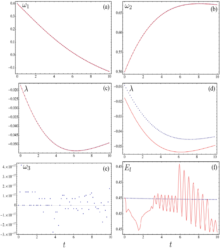
Figure 1. In this figure we display the performance of the midpoint rule ($\overline{\mbox{DSP}}(\omega^{k},\lambda_{k+1};\omega^{k+1})=0$, with inertia matrix $\mathds{I}$ and initial values $\omega_{1}(0)$ and $\omega_{2}(0)$ introduced above) for the nonholonomic rigid body with a time step of size $\epsilon=10^{-3}$. The solid red line is obtained through a RK4 integrator (which we consider an accurate approximation of the continuous nonlinear dynamics over a short time interval), while the blue dots represent the performance of the midpoint rule. The plots $(a)$ and $(b)$ correspond to the dynamical variables $\omega_{1}$, $\omega_{2}$, while $(c)$ displays the Lagrange multipliers $\lambda.$ On the other hand $(d)$ shows the inconsistent multipliers generated by the nonholonomic variational integrator. Finally, $(e)$ and $(f)$ show the preservation of the constraints and the energy $E_{l}(\hat{\omega})$ up through round off errors, respectively.

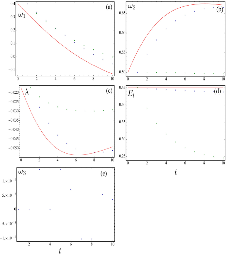
Figure 2. This figure displays the comparison between the midpoint rule (the same as in Figure 1) and the variational integrator (37), (38), for a time step of size $\epsilon=10^{0}=1$ (we recall that this integrator is also order 2 consistent in the dynamical variables). The former is represented by the green points and the latter by the blue ones, while the solid red line still represents the performance of a RK4 method. Variables $\omega_{1}$ $(a)$, $\omega_{2}$ $(b)$, $\lambda$ $(c)$ and $E_{l}$ $(d)$ are displayed, while $(e)$ shows the preservation of the constraints by the variational integrator up through round off errors. We observe a better performance of the variational integrator, mainly with respect to the preservation of energy, a fact which, considering bigger time steps, leads to the conclusion that its convergence to the actual solution is much faster and its long-term behavior is much more accurate.

6. Discretization of the Euler-Poincaré-Suslov problem as perturbation

So far, we have focused on the discretization of the Suslov problem, paying attention to its consistency order and $\mathfrak{so}(3)^{{}_{D}}-$preservation. In this section we return to any Lie group $G$ and its Lie algebra $\mathfrak{g}$, since the relevant results from above apply in this general case as well; in the last part we will particularize $G=SO(3)$.

As it is well-known, by discretizing the dynamics we introduce some discrepancies with respect to the continuous system even when the discretization is performed in some kind of structure-preserving fashion. It is needless to mention that this is a central and fundamental question for all kinds of numerical investigations, especially concerning the long-term evolution of dynamical systems. Regarding this issue, we refer to [13] where a positive answer to the following question is given: Is it possible to embed a numerical scheme approximating the continuous-time flow of a set of autonomous ordinary differential equations (ODE) into the time evolution corresponding to a non-autonomous perturbation of the original autonomous ODE? The positive result may be phrased as: Any $p-$th order discretization of an autonomous ODE can equivalently be viewed as the time$-\epsilon$ period map of a suitable $\epsilon-$periodic non-autonomous perturbation of the original ODE (where $\epsilon$ is the fixed step size of the discretization). The precise statement is:

Theorem 6.1.

Suposse that $h\in C^{r}(\mathds{R}^{n},\mathds{R}^{n})$, $r\geq 1$, and consider the autonomous ODE

$$\dot{x}=h(x).$$ (41)

Let $F(t,x)$ be the solution flow of (41) satisfying $F(0,x)=0,$ and assume that there are an integer $\rho\geq 1$, a continuous function $C:[0,\infty)\rightarrow[0,\infty)$ and a one-step difference approximation of step size $\epsilon$

$$x_{k+1}=\phi(\epsilon,x_{k}),\,\,\,(0<\epsilon\leq\epsilon_{0};\,k\in\mathds{Z})$$

which is consistent of order $p$, i.e.

$$|\phi(\epsilon,x)-F(\epsilon,x)|\leq C(|x|)\,\epsilon^{p+1}.$$

Then, there exists a function $d(\epsilon,t/\epsilon,x)$, as smooth as $h$ and periodic in $t$ of period $\epsilon$, such that if $G(t,s;\epsilon,x)$, $G(s,s;\epsilon,x)=x$, is the solution flow of the non-autonomous, $\epsilon-$periodic ODE

$$\dot{x}=h(x)+\epsilon^{p}d(\epsilon,t/\epsilon,x),$$ (42)

then

$$G(\epsilon,0;\epsilon,x)=\phi(\epsilon,x),$$

where $G(\epsilon,0;\epsilon,\cdot):\mathds{R}^{n}\rightarrow\mathds{R}^{n}$ is the Poincaré map (period map) for (42), corresponding to initial time $s=0$.

Following these ideas, in [15] the case of nonholonomic dynamics in $\mathds{R}^{n}$ has been explored, and the following theorem has been proved. In the context of the present work, i.e. when the configuration manifold is a Lie group, it has to be understood w.r.t. coordinates.

Theorem 6.2.

Let the matrix $\left(\frac{\partial^{2}L}{\partial v^{i}_{g}\partial v^{j}_{g}}\right)$ be positive-definite. Then, any $D-$preserving discretization of the nonholonomic equations (2), the consistency order of which is $p$ w.r.t. the dynamical variables, can be embedded into the time evolution of a non-autonomous perturbation of the following form:

$$\begin{split}\dot{g}^{i}&=v^{i}_{g}+\epsilon^{p}\tilde{d}^{i}_{g}(\epsilon,t/\epsilon,g,v_{g}),\\ \frac{\partial^{2}L}{\partial v^{i}_{g}\partial v^{j}_{g}}\dot{v}^{j}_{g}&=\frac{\partial L}{\partial g^{i}}+\lambda_{\alpha}\,\mu^{\alpha}_{i}(g)+\epsilon^{p}(\tilde{d}_{v_{g}})_{i}(\epsilon,t/\epsilon,g,v_{g}),\\ \mu^{\alpha}_{i}(g)v^{i}_{g}&=0.\end{split}$$ (43)

An analogous result can be obtained in the reduced setting. There are some differences though; first, we note that the differential equations in (9) are of order 1 rather than of order 2 as in (2); second, the constraints $\langle a^{\alpha},\xi\rangle=0$ determine a linear subspace $\mathfrak{g}^{{}_{D}}\subset\mathfrak{g}$ instead of a regular submanifold. The procedure to obtain the perturbation of the nonholonomic dynamics produced by a given discretization can be split into three steps here:

1. Define an ODE evolving on $\mathfrak{g}^{{}_{D}}$ from the Euler-Poincaré-Suslov equations (9) by projection, which we will call Euler-Poincaré-Suslov ODE;

2. Apply Theorem 6.1;

3. Undo the projection process to recover the perturbed Euler-Poincaré-Suslos equations.

Thus, we obtain the following result.

Theorem 6.3.

Let $\left(\frac{\partial^{2}l}{\partial\xi^{a}\partial\xi^{b}}\right)$ be a positive-definite matrix. Any $\mathfrak{g}^{{}_{D}}-$preserving discretization of the Euler-Poincaré-Suslov equations (9), the consistency order of which is $p$ w.r.t. the dynamical part, can be embedded into the time evolution of a non-autonomous perturbation of the following form

$$\begin{split}\frac{\partial^{2}l}{\partial\xi^{b}\partial\xi^{c}}\dot{\xi}^{c}&=C_{be}^{d}\xi^{e}\frac{\partial l}{\partial\xi^{d}}+\lambda_{\alpha}a^{\alpha}_{b}+\epsilon^{p}\tilde{d}_{b}(\epsilon,t/\epsilon,\xi),\\ \langle a^{\alpha},\xi\rangle&=0,\end{split}$$ (44)

where $C_{ab}^{e}$ denote the structure constants of $\mathfrak{g}$ w.r.t. the coordinates chosen.

For convenience, we outline the proof in the appendix. Of course, it would be ideal, if the perturbed Euler-Poincaré-Suslov equations in (44) admitted a Lagrangian structure of some kind. The question, when this is true and how this is related to specific properties of both, the underlying discretization of the unperturbed problem as well as the selected type of embedding, is left as a subject of further study.

7. Conslusions

We followed the ideas presented in [15] to study the discretization of the Suslov problem. First, concerning the order of consistency of discretizations corresponding to the unreduced and reduced settings and related to each other by reduction and reconstruction, respectively, we found that when the discrete reconstruction equation is given by a Cayley retraction map both consistency orders are related to each other, too. The order of consistency carries over unchanged from the unreduced to the reduced setting. It becomes zero in the unreduced setting, no matter how big it is in the reduced setting. Furthermore, we studied distribution preserving integrators, showing that this property may be achieved for general numerical schemes. We presented a specific algorithm with that property based on the general reduced framework. We considered two examples of different integrators, one of them based on the midpoint rule while the other is based on a variational scheme. As proved, both are order-2 consistent in the dynamical variables, but it is numerically shown that the variational one converges faster to the actual solution and shows a better long-term behaviour. Finally, concerning the discretization understood as perturbation, we proved that any distribution preserving integrator of the Euler-Poincaré-Suslov equations (in general) may be understood as a non-autonomous perturbation of the continuous dynamics.

Acknowledgments: We are indebted to the referee for the constructive comments and corrections, which helped a lot to substantially improve the manuscript. We thank Carlos Navarrete-Benlloch for his help in the display of numerical results, and also Dimtry Zenkov and Yuri Fedorov for helpful comments during the “Workshop on Nonholonomic mechanics and optimal control”, held at the Institute Henri Poincaré, Paris, November 2014. The first author is indebted to Luis García-Naranjo for fruitful discussions during their common visit to Technische Universität Berlin. Finally we thank the Deutsche Forschungsgemeinschaft (DFG) for supporting this research within the frame of the project B4 of SFB-Transregio 109 “Discretization in Geometry and Dynamics”.

Appendix: Sketch of the Proof of Theorem 6.3

We first introduce some notation. We set $m\equiv(m_{ab}):=\left(\frac{\partial^{2}l}{\partial\xi^{a}\partial\xi^{b}}\right)$, while $(m^{ab})\equiv m^{-1}$ denotes its inverse (recall that $(m_{ab})$ is regular and positive-definite). With this, the first equation in (9) may be rewritten as

$$\dot{\xi}^{b}=f^{b}(\xi)+\lambda_{\alpha}m^{bc}(a^{\alpha})_{c},$$ (45)

where $f^{b}(\xi):=m^{bc}C^{d}_{ce}\xi^{e}\frac{\partial l}{\partial\xi^{d}}.$

(1) Since $\mu^{\alpha}(g)=\ell^{*}_{g^{-1}}a^{\alpha}$ represent a set of linearly independent one-forms spanning $D_{g}^{\circ}\subset T^{*}_{g}G$, it is easy to see that the $a^{\alpha}$ spanning $(\mathfrak{g}^{{}_{D}})^{\circ}\subset\mathfrak{g}^{*}$ are also linearly independent. Therefore, we can decompose the algebra as

$$\mathfrak{g}=\mathfrak{g}^{{}_{D}}\oplus(\mathfrak{g}^{{}_{D}})^{\perp},$$ (46)

with respect to the metric represented by $(m_{ab})$. Thus, from (45) we can derive an ODE on $\mathfrak{g}^{{}_{D}}$ by eliminating the Lagrange multipliers. More precisely, if we take the time derivative of the nonholonomic constraints we obtain $\langle a^{\alpha},\dot{\xi}\rangle=0$ (note that $a^{\alpha}$ are constant), which, after replacing $\dot{\xi}$ by the right hand side of the equation (45), yields

$$\lambda_{\alpha}(\xi)=-\mathcal{C}_{\alpha\beta}\langle a^{\beta},f(\xi)\rangle,$$ (47)

where $\left(\mathcal{C}^{\alpha\beta}\right):=\left(\langle a^{\alpha},m^{-1}a^{\beta}\rangle\right)$ and $\left(\mathcal{C}_{\alpha\beta}\right)=\mathcal{C}^{-1}.$ It is possible to prove the invertibility of $\mathcal{C}$ using geometric arguments (see for instance [15], lemma 2.4), or just by arguing that $m$ is of full rank and $a^{\alpha}$ of constant rank. Thus, we obtain the Euler-Poincaré-Suslov ODE on $\mathfrak{g}^{{}_{D}}$ given by

$$\dot{\xi}=h(\xi),$$ (48)

with $\langle a^{\alpha},\xi\rangle=0$, where $h(\xi):=f(\xi)+\lambda_{\alpha}(\xi)\,m^{-1}a^{\alpha}$ and $\lambda_{\alpha}(\xi)$ is defined in (47).

(2) Now, let us choose adapted coordinates with respect to the decomposition (46), say $\xi=(\xi^{a})=(\xi^{\bar{a}},\xi^{\hat{a}})$, where $a=1,...,n$, $\bar{a}=1,...,n-m$ (corresponding to $\mathfrak{g}^{{}_{D}}$) and $\hat{a}=n-m+1,...,n$ (corrresponding to $(\mathfrak{g}^{{}_{D}})^{\perp}$). Since $\mathfrak{g}$ is a linear space, the choice of such adapted coordinates is trivial. Projecting (48) onto $\mathfrak{g}^{{}_{D}}$, we obtain

$$\dot{\xi}^{\bar{a}}=h^{\bar{a}}(\bar{\xi}),$$

where we write $\bar{\xi}$ for $(\xi^{\bar{a}})$. Now, we can apply theorem 6.1 to $\dot{\xi}^{\bar{a}}=h^{\bar{a}}(\bar{\xi})$, ensuring that any $p-$th order discretization can be viewed as the time$-\epsilon$ map of a suitable non-autonomous perturbation, which is $\epsilon-$periodic in $t$, namely

$$\dot{\xi}^{\bar{a}}=h^{\bar{a}}(\bar{\xi})+\epsilon^{p}d^{\bar{a}}(\epsilon,t/\epsilon,\bar{\xi}).$$ (49)

(3) This basically finishes the proof, since this equation can be derived from perturbed Euler-Poincaré-Suslov equations of the form

$$\begin{split}\dot{\xi}&=f(\xi)+\lambda_{\alpha}\,m^{-1}a^{\alpha}+\epsilon^{p}\,m^{-1}\,\tilde{d}(\epsilon,t/\epsilon,\xi),\\ \langle a^{\alpha},\xi\rangle&=0.\end{split}$$ (50)

Indeed, we see that the first equation in (50) leads to (49) by eliminating the Lagrange multipliers, which gives

$$\lambda_{\alpha}=\lambda_{\alpha}(\xi)-\epsilon^{p}\mathcal{C}_{\alpha\beta}\langle a^{\beta},\,m^{-1}\tilde{d}\rangle,$$

where $\lambda_{\alpha}(\xi)$ is defined in (47). Plugging this into (50) we finally obtain (49), including as well the identification $d=(d^{\bar{a}})=m^{-1}\tilde{d}-\mathcal{C}_{\alpha\beta}\,m^{-1}\,a^{\alpha}\,\langle a^{\beta},m^{-1}\tilde{d}\rangle$.

This finishes the proof.

References

• [1]
• [2] Arnold VI, Kozlov VV and Neishtadt AI
“Mathematical Aspects of Classical and Celestial Mechanics; Dynamical Systems III”, Springer-Verlag, New York, (1989).
• [3] Bloch AM
“Nonholonomic Mechanics and Control”, Interdisciplinary Applied Mathematics Series 24, Springer-Verlag New-York, (2003).
• [4] Bloch AM, Krishnaprasad PS, Marsden JE and Murray R
“Nonholonomic mechanical systems with symmetry,” Arch. Rational Mech. Anal., 136(1), pp. 21–99, (1996).
• [5] Bobenko AI and Suris YB
“Discrete Lagrangian Reduction, Discrete Euler-Poincaré Equations and Semidirect Products”, Lett. Math. Phys., 49, pp. 79–83, (1999).
• [6] Bou-Rabee N and Marsden JE
“Hamilton-Pontryagin Integrators on Lie Groups: Introduction and Structure-Preserving Properties”, Foundations of Computational Mathematics, 9(2), pp. 197–219, (2009).
• [7] Cantrijn F, de León M, Marrero JC and Martín de Diego D
“Reduction of nonholonomic mechanical systems with symmetry,” Reports on Mathematical Physics, 42(1-2), pp. 25–45, (1998).
• [8] Cortés J and Martínez E
“Nonholonomic integrators”, Nonlinearity, 14(5), pp. 1365–1392, (2001).
• [9] Fedorov YN
“A discretization of the Nonholonomic Chaplygin Sphere Problem”, SIGMA: Symmetry Integrability Geom. Methods Appl., 3, 15 pp, (2007).
• [10] Fedorov YN and Zenkov DV
“Discrete nonholonomic LL systems on Lie groups,” Nonlinearity, 18(5), pp. 2211–2241, (2005).
• [11] Ferraro S, Iglesias D and Martín de Diego, D
“Momentum and energy preserving integrators for nonholonomic dynamics”, Nonlinearity, 21(8), pp. 1911–1928, (2008).
• [12] Ferraro S, Jiménez F and Martín de Diego, D
“New developments on the Geometric Nonholonomic Integrator”, Nonlinearity, 28, pp. 871–900, (2015).
• [13] Fielder B and Scheurle J
“Discretization of homoclinic orbits, rapid forcing and invisible chaos” Memoirs of the American Mathematical Society, 119(570), (1996).
• [14] Hairer E, Lubich C and Wanner G
“Geometric Numerical Integration, Structure-Preserving Algorithms for Ordinary Differential Equations”, Springer Series in Computational Mathematics, 31, Springer-Verlag Berlin, (2002).
• [15] Jiménez F and Scheurle J
“On the discretization of nonholonomic mechanics in $\mathds{R}^{n}$”, Journal of Geometric Mechanics, 7(1), pp. 43–80, (2015).
• [16] Iglesias D, Marrero JC, Martín de Diego and Martínez E
“Discrete Nonholonomic Lagrangian Systems on Lie Groupoids”, Journal of Nonlinear Sciences, 18, pp. 351-397, (2008).
• [17] Kobilarov M, Martín de Diego D and Ferraro S
“Simulating Nonholonomic Dynamics”, Boletín de la Sociedad de Matemática Aplicada SeMA, 50, pp. 61–81, (2010).
• [18] Kozlov VV
“Invariant Measures of the Euler-Poincaré Equations on Lie algebras”, Funct. Anal. Appl., 22, pp. 58–59, (1988).
• [19] de León M
“A historical review on nonholonomic mechanics”, Rev. R. Acad. Ciencias Exactas Fís. Nat. Serie A, 106(1), pp. 191–224, (2012).
• [20] Marsden JE, Pekarsky S and Shkoller S
“Discrete Euler-Poincaré and Lie-Poisson equations”, Nonlinearity, 12(6), pp. 1647–1662, (1999).
• [21] Marsden JE, Pekarsky S and Shkoller S
“Symmetry reduction of discrete Lagrangian mechanics on Lie groups”, Journal of Geometry and Physics, 36(1-2), pp. 140–151, (2000).
• [22] Marsden JE and West M
“Discrete Mechanics and variational integrators”. Acta Numerica, 10, pp. 357–514, (2001).
• [23] McLachlan R and Perlmutter M
“Integrators for Nonholonomic Mechanical Systems.” J. Nonlinear Science, 16, pp. 283–328, (2006).
• [24] Moser J and Veselov AP
“Discrete versions of some classical integrable systems and factorization of matrix polynomials” Comm. Math. Phys. 139, pp. 217–243, (1991).
• [25] Suslov G
“Theoretical Mechanics”, 2, Kiev (in Russian), (1902).
• [26] Weinstein A
“Lagrangian Mechanics and groupoids”, Fields Inst. Comm. 7, pp. 207–231, (1996).