Externally controlled selective spin transfer through a two-terminal bridge setup

Abstract

A new way of getting controlled spin dependent transport through a two-terminal bridge setup is explored. The system comprises a magnetic quantum ring which is directly coupled to a magnetic quantum wire and subjected to an in-plane electric field perpendicular to the wire. Without directly changing system parameters, one can regulate spin currents simply by tuning the external electric field under a finite bias drop across the wire. For some particular field strengths a high degree of spin polarization can be achieved and thus the system can essentially be utilized as an externally controlled spin polarized device. A detailed comparison of spin current magnitudes obtained from other bridge setups is also examined to make the present investigation a self contained study.

I Introduction

The phenomenon of spin polarized transport sp1 ; sp2 ; sp3 in low-dimensional systems has emerged as one of the most promising area over the last few decades in condensed matter physics due to its potential application in nano-science and technology nano1 ; nano2 . The advancement of nano-lithographic techniques along with sophisticated instrumentation facilities have enabled experimentalists to explore spin dependent transport through different tailor made geometries and test their ability in the realization of future nano-scale spin based electronic devices ex1 ; ex2 ; ex3 . With the discovery of giant magneto-resistance (GMR) effect gmr in Fe/Cr magnetic multilayers during 1980’s a new branch in condensed matter physics, the so-called spintronics, has been developed which deals with the possibilities of exploring electron spin in transport properties. This phenomenon has lead to the revolutionary progress in devices making, data processing, quantum computations and many others dev1 ; dev2 ; dev3 ; dev4 . Three most fundamental steps are involved spinsteps1 ; spinsteps2 in designing spin based electronic devices those are: injection of spin through interfaces, propagation of spin through material and finally the detection of spin. Quantum confined nanostructures are the ideal candidates for it since they have considerably large spin coherence time. Therefore, the studies associated with spin dependent transport in nanostructures are of great importance from the aspect of theoretical understanding as well as technological progress, especially to design spintronic devices.

In order to design a controllable spintronic device, the most crucial requirement is the generation of polarized spin currents and proper regulation of these currents. Therefore, modeling of spin filter is of great importance. Over the last few years many theoretical th1 ; th2 ; sm1 ; th3 ; sm2 ; th4 ; thnew1 ; thnew2 ; thnew3 ; thnew4 ; th5 ; th6 ; sm3 ; th7 ; th8 as well as experimental ex1 ; ex2 ; ex3 ; expt works have been done to explore spin dependent transport at nano-scale level and to design efficient spin filter with higher spin polarizability. One common route of developing a spin filter is by using ferromagnetic electrodes trend1 ; trend2 though its experimental realization is somewhat complicated since spin injection from these electrodes becomes quite difficult due to large resistivity mismatch. Keeping in mind the above issue, a large section of the existing literature rather suggests to design spin filter device using the intrinsic properties of materials, for example, spin-orbit (SO) interactions intrinsic1 ; intrinsic2 ; intrinsic3 ; intrinsic4 ; intrinsic5 ; intrinsic6 . Usually two types of SO interactions, Rashba and Dresselhaus, are encountered in solid state materials rashba ; dressel ; winkler ; skm depending on their sources. The Rashba SO coupling in a material is attributed to an electric field that originates from the lacking of structural symmetry whereas, the Dresselhaus SO interaction appears from

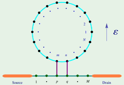
Figure 1: (Color online). A magnetic quantum wire, sandwiched between two one-dimensional non-magnetic source and drain electrodes, is directly coupled to a magnetic quantum ring. An in-plane electric field $\mathcal{E}$, perpendicular to the wire, is applied to the ring.

the bulk inversion asymmetry. Out of these two, Rashba SO interaction has been attracted much attention in the field of spintronics since its coupling strength can be tuned by electrostatic means i.e., applying external gate voltages gt1 ; gt2 ; gt3 ; gt4 ; gt5 which provides controlled spin dependent transport and manipulates electronic spin state. In presence of SO coupling polarized spin currents in output terminals of a multi-terminal conductor can be achieved from a completely unpolarized electron beam injected to its input terminal. To date, many works have been done mlt1 ; mlt2 ; mlt3 ; mlt4 ; mlt5 ; skm3 considering different multi-terminal geometries. For example, in 2006, Peeters et al. have analyzed how a simple mesoscopic ring with one input and two output terminals can be utilized as an electron spin beam splitter mlt1 in presence of Rashba SO coupling. In other work, Kislev and Kim have proposed that a planar T-shaped geometry with a ring resonator provides mlt2 Rashba SO interaction induced polarized spin currents in output terminals. Among these, many other groups mlt3 ; mlt4 have also put forward different key ideas in this particular realm. But, it should be stressed, unlike multi-terminal bridge systems, only SO coupling is incapable of producing polarized spin current when a sample is coupled to single input and a single output lead i.e., in a two-terminal bridge setup mlt2 . In presence of SO coupling the time-reversal symmetry gets preserved, and hence, it doesn’t break Kramer’s degeneracy between $|k\uparrow\rangle$ and $|-k\downarrow\rangle$ states which results vanishing spin current in the output lead. This degeneracy is broken when the material is subjected to an external magnetic field, and under this situation a two-terminal conductor subjected to SO interaction can exhibit raba ; smpola polarized spin current in its output lead. But, this approach is not quite suitable since confining a strong magnetic field in a small region like a quantum dot (QD) or a quantum ring (QR) is extremely difficult. Therefore, further studies are still required to develop a possible route of getting controlled spin selective transmission in a two-terminal geometry.

In the present paper, we propose a theoretical model to realize spin selective transmission through a two-terminal conducting bridge and explore the possibilities to control spin dependent currents externally without directly changing the physical parameters of the system. The model quantum system is designed by a magnetic quantum wire (MQW), sandwiched between two non-magnetic (NM) source and drain electrodes, which is again directly coupled to a magnetic quantum ring (MQR). The ring is subjected to an external electric field and it is the key controlling parameter of our present investigation. The main motivation behind the consideration of this particular geometry is to investigate the interplay of the MQR, which behaves like a correlated disordered ring in presence of external electric field (will be discussed later in the appropriate sub-section), and the MQW to achieve selective spin transport in a two-terminal junction. It is well known that in any magnetic nanostructure there is always a band misalignment between up and down spin electrons irrespective of any external electric field, and therefore, one can get pure spin current upon selecting the Fermi energy to a suitable energy zone. But, for such a nanostructure neither spin current can be controlled efficiently nor large spin current can be achieved. To circumvent these issues we propose a new model, shown in Fig. 1, where spin current can be tuned systematically by means of external electric field and controlling this field large current can be achieved. We strongly believe that the design of such a system is of great concern in the current era of nanofabrication. Within a tight-binding (TB) framework and based on Green’s function formalism we show that selective spin currents are available at the output terminal and their magnitudes can be regulated by means of external in-plane electric field. This system also exhibits a high degree of spin polarization for some typical field strengths. Our theoretical results promote practical applications of externally controlled spin polarized quantum devices. Finally, to substantiate the proposed system as an efficient two-terminal externally controlled spin-filter device, here we also compare the spin current magnitudes considering other geometrical systems. Analyzing the results we ensure that the model presented in Fig. 1 is the most suitable one.

The rest of the paper is organized as follows. In Section II we describe the model together with theoretical formulations for the calculations. Essential findings are described in Section III. Finally, we summarize our results in Section IV.

II Model and theoretical framework

II.1 Model and Hamiltonian

Let us begin by referring to Fig. 1 where a MQW, coupled to a MQR, is sandwiched between two semi-infinite one-dimensional NM electrodes commonly known as source and drain. The ring is subjected to an in-plane electric field $\mathcal{E}$, perpendicular to the wire, which controls selective spin transmission across this two-terminal junction. To emphasize the effect of quantum interference on electronic transport we connect the ring to the wire through two vertical bonds, instead of attaching them via a single bond.

Using a tight-binding approach we describe the model quantum system and in the absence of any electron-electron (e-e) interaction this scheme is extremely suitable for analyzing electron transport through a conducting bridge tb1 ; tb2 ; tb3 ; tb4 ; tb5 ; tb6 ; tb7 ; tb8 . The single particle TB Hamiltonian that includes the MQW, MQR and NM source and drain electrodes can be written as,

$$H=H_{\mbox{\tiny c}}+H_{\mbox{\tiny el}}+H_{\mbox{\tiny tn}}$$ (1)

where three different terms in the right side represent three distinct regions of the complete system. These terms are elaborately explained as follows.

The first term $H_{\mbox{\tiny c}}$ corresponds to the Hamiltonian of the conductor within the electrodes i.e., the ring including the wire. Each site of the ring as well as the wire is associated with a local magnetic moment with amplitude $h_{i}$ (say, for $i$-th site) and the orientation of such a magnetic moment is specified by the polar angle $\theta_{i}$ and azimuthal angle $\phi_{i}$ in spherical polar co-ordinate system. The orientations of these local moments can be controlled by applying a magnetic field. Under nearest-neighbor hopping approximation the TB Hamiltonian $H_{\mbox{\tiny c}}$ becomes,

$$H_{\mbox{\tiny c}} = \sum_{i}\mbox{\boldmath$c$}_{i}^{r\dagger}\left(\mbox{\boldmath$\epsilon$}_{i}^{r}-\vec{\mbox{\boldmath$h$}}_{i}.\vec{\sigma}\right)\mbox{\boldmath$c$}_{i}^{r}+\sum_{i}\left(\mbox{\boldmath$c$}_{i+1}^{r\dagger}\mbox{\boldmath$t$}_{r}\mbox{\boldmath$c$}_{i}^{r}+h.c.\right)$$ (2)

$$+ \sum_{i}\mbox{\boldmath$c$}_{i}^{w\dagger}\left(\mbox{\boldmath$\epsilon$}_{i}^{w}-\vec{\mbox{\boldmath$h$}}_{i}.\vec{\sigma}\right)\mbox{\boldmath$c$}_{i}^{w}+\sum_{i}\left(\mbox{\boldmath$c$}_{i+1}^{w\dagger}\mbox{\boldmath$t$}_{w}\mbox{\boldmath$c$}_{i}^{w}+h.c.\right)$$

$$+ \left(\mbox{\boldmath$c$}_{m}^{r\dagger}\mbox{\small\boldmath$\lambda$}\mbox{\boldmath$c$}_{p}^{w}+\mbox{\boldmath$c$}_{n}^{r\dagger}\mbox{\small\boldmath$\lambda$}\mbox{\boldmath$c$}_{q}^{w}+h.c.\right)$$

where,
$\mbox{\boldmath$c$}_{i}^{r\dagger}=\left(\begin{array}[]{cc}c_{i\uparrow}^{r\dagger}&c_{i\downarrow}^{r\dagger}\end{array}\right);$ $\mbox{\boldmath$c$}_{i}^{r}=\left(\begin{array}[]{c}c_{i\uparrow}^{r}\\ c_{i\downarrow}^{r}\end{array}\right);$ $\mbox{\boldmath$c$}_{i}^{w\dagger}=\left(\begin{array}[]{cc}c_{i\uparrow}^{w\dagger}&c_{i\downarrow}^{w\dagger}\end{array}\right);$ $\mbox{\boldmath$c$}_{i}^{w}=\left(\begin{array}[]{c}c_{i\uparrow}^{w}\\ c_{i\downarrow}^{w}\end{array}\right);$ $\mbox{\boldmath$\epsilon$}_{i}^{r}=\left(\begin{array}[]{cc}\epsilon_{i}^{r}&0\\ 0&\epsilon_{i}^{r}\end{array}\right);$ $\mbox{\boldmath$\epsilon$}_{i}^{w}=\left(\begin{array}[]{cc}\epsilon_{i}^{w}&0\\ 0&\epsilon_{i}^{w}\end{array}\right);$
$\mbox{\boldmath$t$}_{r}=t_{r}\left(\begin{array}[]{cc}1&0\\ 0&1\end{array}\right);$ $\mbox{\boldmath$t$}_{w}=t_{w}\left(\begin{array}[]{cc}1&0\\ 0&1\end{array}\right);$ $\mbox{\small\boldmath$\lambda$}=$$\lambda$$\left(\begin{array}[]{cc}1&0\\ 0&1\end{array}\right);$ $\vec{\mbox{\boldmath$h$}}_{i}.\vec{\sigma}=h_{i}\left(\begin{array}[]{cc}\cos\theta_{i}&\sin\theta_{i}e^{-j\phi_{i}}\\ \sin\theta_{i}e^{j\phi_{i}}&-\cos\theta_{i}\end{array}\right).$
 
In the above expression (Eq. 2), the 1st and 2nd terms are associated with the magnetic quantum ring of $N$ atomic sites, whereas for the magnetic wire containing $M$ atomic sites the 3rd and 4th terms are used, and the last term describes the coupling between them. $c_{i\sigma}^{r\dagger}$ and $c_{i\sigma}^{r}$ are the creation and annihilation operators, respectively, for an electron with spin $\sigma(\uparrow,\downarrow)$ at the site $i$ of the ring, while for the wire they are represented by $c_{i\sigma}^{w\dagger}$ and $c_{i\sigma}^{w}$, respectively. $\epsilon_{i}^{r}$ gives the site energy and $t_{r}$ corresponds to the nearest-neighbor hopping integral in the ring. Similarly, for the wire they are respectively described by $\epsilon_{i}^{w}$ and $t_{w}$. The factor $\vec{\mbox{\boldmath$h$}}_{i}.\vec{\sigma}$ describes interaction of the spin of injected electron to the local magnetic moment placed at $i$-th site. In order to elucidate the role of quantum interference on electronic conduction, MQR is attached to the MQW by more than a single interaction, as shown in Fig. 1. Any two atomic sites $m$ and $n$ (not necessarily nearest-neighbor) of the MQR can be connected to the atomic sites $p$ and $q$ of the MQW by two vertical lines to get two different connecting paths between the MQR and MQW. As the essential features of our present investigation can be acquired considering $m$ and $n$ as nearest-neighbor sites (the simplest configuration), we couple the site $m$ of the MQR to the site $p$ of the MQW by a single bond, and similarly, the site $n$ is connected to the site $q$ by another bond (Fig. 1, for this configuration $p$ and $q$ are also the nearest-neighbor sites). The hopping integral between the sites $m$ and $p$ is described by the parameter $\lambda$, and for the other two sites $n$ and $q$ it is also characterized by $\lambda$. The main target of this particular geometry is to find the selective and controlled spin transmission and the interplay of energy levels of the ring which is coupled to a quantum wire in presence of a finite bias. This can essentially be done with the help of external electric field which regulates on-site potentials of MQR upon the variation of electric field. In presence of this field, site energy of the MQR becomes field dependent and doing some simple and straight-forward mathematical steps one can get the site energy for a $N$-site ring as: $\epsilon_{i}^{r}=(eaN\mathcal{E}/2\pi)\cos[2\pi(i-1)/N]$, where $e$ gives the electronic charge, $a$ corresponds to the lattice spacing and $\mathcal{E}$ measures the electric field strength. This relation can be simplified by introducing the dimensionless electric field strength $\xi$ as $\epsilon_{i}^{r}=\left(Nt_{w}\xi/2\pi\right)\cos[2\pi(i-1)/N]$, where $\xi=ea\mathcal{E}/t_{w}$. In absence of any electric field, local on-site energy $\epsilon_{i}^{r}$ of the ring becomes constant, and therefore, we can fix it at zero without loss of any generality. This is exactly what we get from the above relation.

The side attached electrodes are assumed to be semi-infinite, non-magnetic and free from any kind of impurities. We can express them like,

$$H_{\mbox{\tiny el}}=\sum_{\alpha}H_{\alpha}$$ (3)

where $\alpha=S$ and $D$ for the source and drain, respectively. In TB framework $H_{\alpha}$ reads as,

$$H_{\alpha}=\sum\limits_{i}\mbox{\boldmath$d$}_{i}^{\dagger}\mbox{\boldmath$\epsilon$}_{l}^{\alpha}\mbox{\boldmath$d$}_{i}+\sum_{i}\left(\mbox{\boldmath$d$}_{i}^{\dagger}\mbox{\boldmath$t$}_{l}^{\alpha}\mbox{\boldmath$d$}_{i+1}+h.c.\right)$$ (4)

with $\mbox{\boldmath$\epsilon$}_{l}^{\alpha}=\epsilon_{l}^{\alpha}\left(\begin{array}[]{cc}1&0\\ 0&1\end{array}\right)$ and $\mbox{\boldmath$t$}_{l}^{\alpha}=t_{l}^{\alpha}\left(\begin{array}[]{cc}1&0\\ 0&1\end{array}\right)$.
 
$\epsilon_{l}^{\alpha}$ and $t_{l}^{\alpha}$ are the site energy and nearest-neighbor hopping integral, respectively, in the $\alpha$-th lead, and $d_{i\sigma}^{\dagger}$ ($d_{i\sigma}$) is the creation (annihilation) operator of an electron with spin $\sigma$ at $i$-th site of the electrodes. These electrodes are coupled through the atomic sites $1$ and $M$ of the wire via the coupling parameter $t_{c}$. Following the same prescription the wire-to-lead coupling Hamiltonian gets the form,

$$H_{\mbox{\tiny tn}}=\mbox{\boldmath$c$}^{w\dagger}_{1}\mbox{\boldmath$t$}_{c}\mbox{\boldmath$d$}_{0}+\mbox{\boldmath$d$}_{0}^{\dagger}\mbox{\boldmath$t$}_{c}\mbox{\boldmath$c$}^{w}_{1}+\mbox{\boldmath$c$}_{M}^{w\dagger}\mbox{\boldmath$t$}_{c}\mbox{\boldmath$d$}_{M+1}+\mbox{\boldmath$d$}_{M+1}^{\dagger}\mbox{\boldmath$t$}_{c}\mbox{\boldmath$c$}^{w}_{M}$$ (5)

with $\mbox{\boldmath$t$}_{c}=t_{c}\left(\begin{array}[]{cc}1&0\\ 0&1\end{array}\right).$

II.2 Transmission probability, junction current and spin polarization coefficient: Green’s function approach

To calculate spin dependent transmission probabilities, junction currents and spin polarization coefficient we use Green’s function formalism datta1 ; datta2 . In this approach, transmission probability $T_{\sigma\sigma^{\prime}}$ of an injecting electron with spin $\sigma$ which gets transmitted through the drain electrode with spin $\sigma^{\prime}$ is written as datta1 ; datta2 $T_{\sigma\sigma^{\prime}}=\mbox{Tr}\left[\Gamma_{\mbox{\tiny S}}^{\sigma}G_{c}^{r}\Gamma_{\mbox{\tiny D}}^{\sigma^{\prime}}G_{c}^{a}\right]$. When $\sigma=\sigma^{\prime}$ we get pure spin transmission, while for the other case ($\sigma\neq\sigma^{\prime}$) spin flip transmission is obtained. $G_{c}^{r}$ and $G_{c}^{a}$ are the retarded and advanced Green’s functions, respectively, of the conductor i.e., MQR including the MQW sandwiched between the electrodes. $G_{c}^{r}=\left(E-H_{\mbox{\tiny c}}-\sum\limits_{\sigma}\Sigma_{\mbox{\tiny S}}^{\sigma}-\sum\limits_{\sigma}\Sigma_{\mbox{\tiny D}}^{\sigma}\right)^{-1}$, where $E$ is the energy of an injecting electron, and $\Sigma_{\mbox{\tiny S}}^{\sigma}$ and $\Sigma_{\mbox{\tiny D}}^{\sigma}$ are the self-energies due to coupling of the MQW to the electrodes and $\Gamma_{\mbox{\tiny S}}^{\sigma}$ and $\Gamma_{\mbox{\tiny D}}^{\sigma}$ are their imaginary parts. For comprehensive derivations of these self-energy matrices, go through the references datta1 ; datta2 . In these pioneering references it is shown that the self-energy can be expressed as a linear combination of real and imaginary parts, where the real part measures the shift of energy levels, while the other part gives the broadening of these levels. The finite imaginary part appears due to incorporation of the semi-infinite electrodes having continuous energy spectrum.

The spin dependent current $I_{\sigma\sigma^{\prime}}$ passing through the junction can be obtained from the Landauer-Büttiker formalism. It is written as datta1 ; datta2 ,

$$I_{\sigma\sigma^{\prime}}(V)=\frac{e}{h}\int\left[f_{\mbox{\tiny S}}(E)-f_{\mbox{\tiny D}}(E)\right]T_{\sigma\sigma^{\prime}}(E)\,dE$$ (6)

where, $f_{\mbox{\tiny S}}(E)$ and $f_{\mbox{\tiny D}}(E)$ are the Fermi distribution functions of the source and drain with electro-chemical potentials $\mu_{\mbox{\tiny S}}$ ($=E_{F}+eV/2$) and $\mu_{\mbox{\tiny D}}$ ($=E_{F}-eV/2$), respectively. $E_{F}$ gives the equilibrium Fermi energy and it can be controlled via external gate voltages. From Eq. 6 we can evaluate pure spin currents (up spin electron gets transmitted as up spin, and similarly for down spin electron which is transferred as a down spin) as well as spin flip currents (up spin electron gets flipped when it reaches to the drain through the bridging magnetic conductor and vice versa) by integrating proper transmission coefficients over a particular voltage window, and eventually, we obtain the net up and down spin currents. These are: $I_{\uparrow}=I_{\uparrow\uparrow}+I_{\downarrow\uparrow}$ and $I_{\downarrow}=I_{\downarrow\downarrow}+I_{\uparrow\downarrow}$.

Finally, spin polarization coefficient of total current is measured from the relation rai ; nmn ,

$$P = \left|\frac{I_{\uparrow}-I_{\downarrow}}{I_{\uparrow}+I_{\downarrow}}\right|$$ (7)

$$= \left|\zeta_{\uparrow}-\zeta_{\downarrow}\right|$$

where, $\zeta_{\sigma}=I_{\sigma}/(I_{\uparrow}+I_{\downarrow})$ describes the spin filter efficiency. The quantities $I_{\uparrow}$ and $I_{\downarrow}$ can also be derived directly from Eq. 6 by integrating the net up and down spin transmission probabilities those are respectively expressed as $T_{\uparrow}=T_{\uparrow\uparrow}+T_{\downarrow\uparrow}$ and $T_{\downarrow}=T_{\downarrow\downarrow}+T_{\uparrow\downarrow}$. In our theoretical description all the mathematical expressions are framed considering the quantization direction along the positive z-axis where $\sigma_{z}$ gets the form:

$$\sigma_{z}=\left(\begin{array}[]{cc}1&0\\ 0&-1\end{array}\right).$$

III Numerical results and discussion

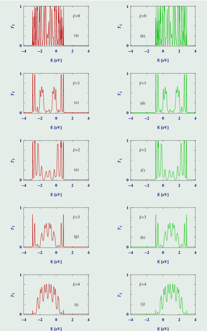
Figure 2: (Color online). Energy dependence of $T_{\uparrow}$ and $T_{\downarrow}$ for different values of dimensionless electric field strength $\xi$. The other physical parameters are: $N=42$, $M=20$, $m=32$, $n=33$, $p=10$, $q=11$ and $\lambda=1$ eV.

According to the above theoretical formulation, described in Sec. II, we are now ready to present our numerical results for spin dependent transmission probabilities and spin polarization coefficient, and, the effect of in-plane electric field on them. During calculations we fix the electronic temperature of the system to zero. The other common parameters are chosen as follows. Both in the MQW and MQR we assume that all the magnetic moments are aligned along positive z-axis i.e., $\theta_{i}=0$ and $\phi_{i}=0$ and they are equal in magnitude ($h_{i}=1$ eV for all the magnetic sites $i$). The site energies in the electrodes ($\epsilon_{l}^{\alpha}$) and in the magnetic wire ($\epsilon_{i}^{w}$) are set to zero. For the ring, the site energies ($\epsilon_{i}^{r}$) are no longer identical since they are field dependent for non-zero electric field as prescribed in our theoretical description. The hopping integrals $t_{r}$, $t_{w}$ and $t_{c}$ are set to $1$ eV, whereas the hopping integral in the electrodes $t_{l}^{\alpha}$ is fixed at $2$ eV. Finally, we set the lattice spacing $a=1\,A^{\circ}$.

III.1 Two-terminal transmission coefficients

We start by analyzing the influence of in-plane electric field on transmission probabilities. The results for net up ($T_{\uparrow}$) and down ($T_{\downarrow}$) spin transmission probabilities as a function of injecting electron energy $E$ are depicted in Fig. 2, where sizes of the MQR and MQW are chosen as $N=42$ and $M=20$, respectively, and the other physical parameters are set at $m=32$, $n=33$, $p=10$, $q=11$ and $\lambda=1$ eV. The transmission spectra exhibit several interesting patterns both for up and down spin electrons which are analyzed as follows. In absence of external electric field the transmission coefficients $T_{\uparrow}$ and $T_{\downarrow}$ provide sharp resonant peaks (see Figs. 2(a) and (b)) associated with energy eigenvalues of the conductor, and for most of these resonant energies the transmission probability reaches very close to unity. The transmittance spectrum gets significantly modified with external electric field and depending on its strength, low and high, two anomalous features are obtained. At lower value of $\xi$, say $\xi=1$, resonant peaks are broadened and they are separated with non-uniform energy gaps (see Figs. 2(c) and (d)). In addition, the heights of some of these resonant peaks are also suppressed compared to the electric field free case, which is noticed by comparing the spectra shown in the top two rows of Fig. 2. With increasing the field strength, say $\xi=2$, some resonant peaks with larger widths (Figs. 2(e) and (f)) are generated across the edges of allowed energy band, but around the energy band centre height of the peaks is reduced enormously. If the field strength is increased further, the features described above get reversed. More resonant peaks appear around the energy band centre with increasing heights (Figs. 2(g) and (h)) and for large enough field strength gapless spectrum is visible (Figs. 2(i) and (j)).

Now we try to explain these spectral features physically. The transmission spectrum of a bridge system is directly associated with eigenenergies of the conductor clamped between two electrodes. In absence of any electric field, the conductor within the electrodes behaves like a perfect one since site energies of both the MQR and MQW are identical. For such a perfect conductor the energy levels are conducting in nature and all of them contribute to the electronic transmission which results a large number of resonant peaks in $T_{\sigma}$-$E$ spectrum. For non-zero electric field, site energies of the MQR are no longer identical to the MQW since they are now field dependent and none of them are equal in magnitude. Under this situation the MQR is treated as a correlated disordered ring and hence the combined system (MQW including MQR) within the electrodes can be called as an ordered-disordered coupled conductor. In a fully disordered system where all site energies are different localized energy states are expected and they become more localized with increasing the disorderness. While, for an ordered-disordered coupled system a set of conducting states together with localized energy levels are obtained and these conducting states become less conducting with increasing disorderness in the weak disorder regime since these two regions are coupled with each other. The situation is somewhat different in the limit of strong disorder. In this limit, the ordered and disordered regions are almost decoupled from each other, and accordingly, the conducting states which arise from the perfect region i.e., MQW are influenced very weakly by the localized states generated from the MQR. With these peculiar features of energy eigenstates in an ordered-disordered coupled system, depending on the strength of disorderness associated with in-plane electric field, the characteristics properties of $T_{\sigma}$-$E$ shown in Fig. 2 can be easily understood. For the lower field strength, less conducting states those are affected by the disordered region contribute to the electronic conduction providing few resonant peaks with reduced amplitudes in the $T_{\sigma}$-$E$ spectrum. On the other hand, for large enough electric field electrons get transmitted only through the perfect region (MQW), and therefore, a gapless spectrum with larger amplitude is obtained.

In addition to the above facts it is interesting to note that the up and down spin electrons are allowed to move through distinct energy channels for a wide range of energy which is observed from the spectra given in Fig. 2. The term $\vec{\mbox{\boldmath$h$}}_{i}.\vec{\sigma}$ in the TB Hamiltonian (Eq. 2) is responsible for it and this channel separation suggests us to design the system as a spin filter which we discuss in the forthcoming sub-section. Before that, here we explain the reason behind the channel separation and approximate the magnitude of misalignment of two different energy bands for up and down spin electrons. As already discussed, the transmission characteristic is the net effect of the combined system where MQW is coupled to the MQR. In absence of any external electric field both these two regions contribute to the transmission for their full allowed energy bands since under this condition all the energy levels are conducting in nature. But, as the electric field is switched on the energy eigenstates associated with the MQR start to localize and even for very weak electric field the contributions from these states almost cease to zero (which can be clearly visible from Fig. 15. Then, the essential contribution comes only from the MQW. Thus, both the nature and width of the $T_{\sigma}$-$E$ spectrum are eventually be controlled by the electric field $\xi$. In order to understand precisely the role of $\xi$ in determining the widths of $T_{\sigma}$-$E$ spectrum we have to focus on the nature of energy band widths of the individual systems i.e., MQR and MQW, since depending on $\xi$ either one (for strong $\xi$) or both of them (for weak $\xi$) contribute to electronic transmission. It is well known that for an ordered one-dimensional non-magnetic tight-binding ring characterized by on-site potential $\epsilon$ (say) and nearest-neighbor hopping integral $t$ (say), the allowed energy band lies within the range $\epsilon-2t$ to $\epsilon+2t$. Similar energy band is also obtained for an infinite one-dimensional perfect chain characterized by these parameters. Using this analogy we can figure out the energy band widths and also the widths of $T_{\sigma}$-$E$ spectra for the sub-systems MQR and MQW including the combined system within the electrodes. To do this we start with the term $\vec{\mbox{\boldmath$h$}}_{i}.\vec{\sigma}$ which becomes $h_{z}.\sigma_{z}$, since in our formulation we assume that all the magnetic moments are equal in magnitude ($h_{i}=h$ (say) for all $i$) and they are aligned along the positive z-axis. Now, at $\xi=0$, $\epsilon_{i}^{r}=0$ for all $i$ of the MQR which results a perfect ring, While, the other part i.e., MQW always behaves like a perfect wire irrespective of $\xi$. This simplification helps us to predict the energy band widths of the sub-systems as follows. For the MQR the range of up spin band is: $-h-2t_{r}$ to $-h+2t_{r}$ and for down spin it is: $h-2t_{r}$ to $h+2t_{r}$. While for the MQW, these are approximately as: $-h-2t_{w}$ to $-h+2t_{w}$ and $h-2t_{w}$ to $h+2t_{w}$, respectively. Therefore, for the chosen set of parameter values the up spin bands for the individual geometries lie within the range $-3$ eV to $1$ eV, and the range becomes $-1$ eV to $3$ eV for the down spin bands. When these two sub-systems i.e., MQR and MQW couple to each other (by the coupling parameter $\lambda$ which is fixed at $1$ eV) to form a combined system, the above energy bands shift a very little and it results a net energy shift $\sim 2h$ ($=2$ eV). This is exactly reflected in the $T_{\sigma}$-$E$ spectra. Certainly, for the non-zero electric field the allowed energy bands get shifted, but then the essential contribution to the electronic transmission comes from the MQW only which results a separation of the order of $2h$ i.e., $2$ eV between the $T_{\uparrow}$-$E$ and $T_{\downarrow}$-$E$.

III.2 Spin dependent currents and spin polarization coefficient for different system sizes

Now, we turn to analyze the variation of spin dependent currents together

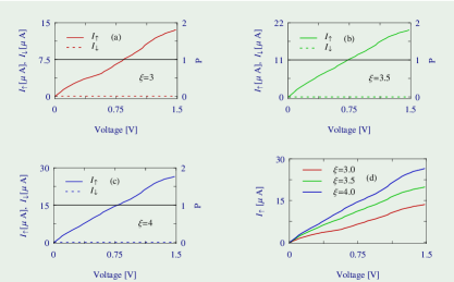
Figure 3: (Color online). (a)-(c): Voltage dependence of up ($I_{\uparrow}$, left axis) and down ($I_{\downarrow}$, left axis) spin currents together with spin polarization coefficient ($P$, right axis, shown by the black curve) for different values of dimensionless electric field strength $\xi$ when the Fermi energy is fixed at $E_{F}=-1.75$ eV. The up spin currents shown in (a)-(c) are placed together in (d) for a better comparison of the amplitudes at different field strengths. The other physical parameters are: $N=42$, $M=20$, $m=32$, $n=33$, $p=10$, $q=11$ and $\lambda=1$ eV.

with spin polarization coefficient and the role of external electric field on them for different sizes of the MQR and MQW. With these characteristics the basic features of electron transmission can be understood in a much deeper way.

As illustrative example, in Fig. 3 we plot the spin dependent

Figure 4: (Color online). (a)-(c): Voltage dependence of up ($I_{\uparrow}$, left axis) and down ($I_{\downarrow}$, left axis) spin currents together with spin polarization coefficient ($P$, right axis, shown by the black curve) for different values of $\xi$ considering $E_{F}=1.75$ eV. The down spin currents shown in (a)-(c) are framed together in (d) for a better comparison of the amplitudes at different field strengths. All the other physical parameters remain exactly identical as taken in Fig. 3.

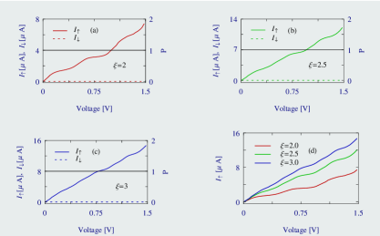
Figure 5: (Color online). (a)-(c): $I_{\uparrow}$ (left axis), $I_{\downarrow}$ (left axis) and $P$ (right axis, shown by the black line) as a function of bias voltage $V$ for different values of $\xi$ taking $E_{F}=-1.75$ eV. The up spin currents shown in (a)-(c) are put together in (d) to compare the current amplitudes properly. The other parameters are: $N=100$, $M=40$, $m=75$, $n=76$, $p=20$, $q=21$ and $\lambda=1$ eV.

currents $I_{\uparrow}$ and $I_{\downarrow}$, and spin polarization coefficient $P$ as a function of applied bias voltage for different field strengths when the Fermi energy is kept fixed at $E_{F}=-1.75$ eV. The results computed for three distinct values of dimensionless electric field strength $\xi$ are shown in (a)-(c), and finally, the up spin currents presented in these three spectra are placed together in (d) to compare their amplitudes properly at different field strengths. From the spectra it is observed that the current for down spin electrons drops exactly to zero (dotted curve) for the entire voltage region, while a finite current (solid curve) is obtained for the other spin electrons. It reveals that electrons with only up spin are allowed to move from the source to drain through the conductor, whereas down spin electrons are totally blocked. The reason is that, setting the Fermi energy at $E_{F}=-1.75$ eV when we apply bias voltage only up spin channels appear within the voltage window and they contribute to the current, but no conducting channel for down spin electrons is available which yields a vanishing down spin current. This phenomenon leads to the possibility of getting spin filtering action

Figure 6: (Color online). (a)-(c): $I_{\uparrow}$ (left axis), $I_{\downarrow}$ (left axis) and $P$ (right axis, shown by the black line) for different values of $\xi$ setting $E_{F}=1.75$ eV. For a better comparison of current amplitudes, the down spin currents shown in (a)-(c) are put together in (d). All the other physical parameters kept unchanged as taken in Fig. 5.

using this bridge setup. The efficiency of spin filtration is depicted by the polarization curve which shows $P=1$ throughout the bias window. This is expected since for the bias window down spin current ceases exactly to zero, while finite up spin current is obtained which yields perfect spin polarization (as clearly seen from Eq. 7). Thus, our proposed quantum system can be utilized as a perfect spin filter for a wide voltage window.

The effect of in-plane electric field on spin current is quite interesting. For a fixed conductor-to-electrode coupling, described by the physical parameter $t_{c}$, the up spin current is enhanced significantly with increasing the dimensionless field strength $\xi$ (see Fig. 3(d)). This enhancement of current amplitude can be attributed following the transmittance-energy spectra (left column of Fig. 2) since current is evaluated by integrating the transmission function (Eq. 6). The area under the transmission curve gets increased with the field strength which results larger current across the bridge system. Usually, the current enhancement takes place by the coupling parameter $t_{c}$ in any bridge system datta1 ; datta2 ; skm1 ; skm2 , but in our setup

Figure 7: (Color online). Voltage dependence of up ($I_{\uparrow}$, left axis) and down ($I_{\downarrow}$, left axis, dotted line) spin currents together with spin polarization coefficient ($P$, right axis) for different values of the ring to wire coupling strength $\lambda$ when $E_{F}=-1.85$ eV. The other parameters are: $N=150$, $M=50$, $m=113$, $n=114$, $p=25$ and $q=26$.

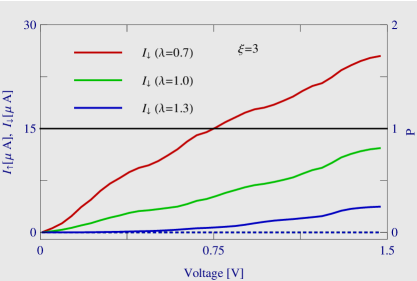
Figure 8: (Color online). Voltage dependence of up ($I_{\uparrow}$, left axis) and down ($I_{\downarrow}$, left axis, dotted line) spin currents together with spin polarization coefficient ($P$, right axis) for different values of $\lambda$ setting $E_{F}=1.85$ eV. The other parameters are same as taken in Fig. 7.

we perform it externally with the help of in-plane electric field without directly changing other physical parameters of the system. It emphasizes that the presented system can be utilized as an externally controlled spin based quantum device.

An exactly similar behavior is also obtained for the down spin electrons when we set the Fermi energy $E_{F}=1.75$ eV. The variation of up and down spin currents along with the spin polarization coefficient are presented in Fig. 4 considering the identical parameter values as taken in Fig. 3. From the spectra illustrated in Figs. 3 and 4 we can predict that by tuning the Fermi energy to a suitable energy zone selective spin transfer can be achieved through our proposed two-terminal bridge setup.

The characteristic features of spin resolved currents ($I_{\uparrow}$ and $I_{\downarrow}$) including the spin polarization coefficient ($P$) as a function of external bias for other system sizes of the MQR and MQW are qualitatively similar to those with the bridge setup where $N$ and $M$ are fixed at $42$ and $20$, respectively (Figs. 3 and 4). The results are presented in Figs. 5 and 6 for different strengths of the dimensionless electric field $\xi$ and they are worked out for $N=100$ and $M=40$. Observations of these spin dependent currents together with spin polarization for different system sizes (see Figs. 3-6) clearly suggest that the results are quite robust, and thus, can be utilized to achieve spin selective currents as well as high degree of spin polarization in a two-terminal geometry.

III.3 Effect of $\lambda$ on spin currents and spin polarization coefficient

In order to elucidate the role played by the ring-to-wire coupling $\lambda$ on spin polarization and spin selective transmissions, in Figs. 7 and 8 we present the results for a bridge setup with $N=150$ and $M=50$ considering different values of $\lambda$. In Fig. 7 the results are shown when the Fermi energy is fixed at $E_{F}=-1.85$ eV, while it is $1.85$ eV for the other figure (Fig. 8). From the spectra it is observed that the selective spin current (up or down), associated with the choice of Fermi energy, gradually decreases with increasing the strength $\lambda$. In presence of finite electric field, the coupling between the ordered (MQW) and disordered (MQR) regions gets enhanced with increasing the coupling parameter $\lambda$. Therefore, the ordered states generated from the MQW are more affected by the disordered states appearing from the MQR for higher $\lambda$ which results lower current. All the other characteristic features remain qualitatively similar to those as discussed in the previous sub-section.

III.4 Practicability consideration: Comparison of spin current amplitudes for the zero and non-zero electric field cases

To demonstrate the crucial role of external electric field on regulation of spin current amplitude across the junction shown in Fig. 1, now it is interesting to compare spin dependent currents computed for zero and non-zero field cases. First we focus on the results given in Fig. 9 where spin dependent currents are computed for two different field strengths, $\xi=0$ and $\xi=3$, setting the Fermi energy $E_{F}=-1.85$ eV. The results are very significant. For $\xi=0$, the up spin current becomes two small (solid blue line), while it rises to a large value for the non-zero field (green line). This enhancement of current amplitude can be justified from our previous analysis. As noted in sub-section B, we see that in the zero field limit both the MQR and MQW contribute to the current where the transmission spectrum exhibits sharp resonant peaks which provide a sufficiently small current upon integrating the transmission function. On the other hand, for non-zero and moderate field strengths transmittance-energy spectrum looks like as obtained in a conventional magnetic wire with broader resonant peaks which results a larger current across the junction.

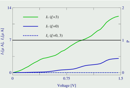
Figure 9: (Color online). Comparison between up spin currents (left axis) for zero and non-zero field cases is shown considering $E_{F}=-1.85$ eV. The variations of down spin currents (left axis) together with spin polarization coefficient (right axis) are also presented. Here we choose $N=150$, $M=50$, $m=113$, $n=114$, $p=25$, $q=26$ and $\lambda=1$ eV.

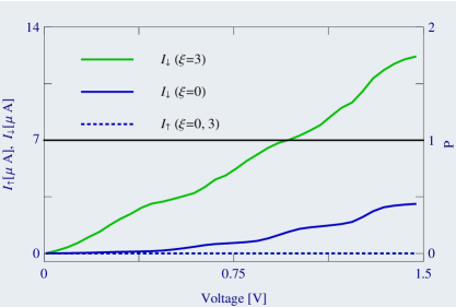
Figure 10: (Color online). Comparison between down spin currents (left axis) for zero and non-zero field cases is shown considering $E_{F}=1.85$ eV. The variations of up spin currents (left axis) together with spin polarization coefficient (right axis) are also presented. All the other parameters are same as in Fig. 9.

The nature of vanishing down spin currents and perfect spin polarization shown in this figure (Fig. 9) can be easily understood from the earlier analysis.

Similar arguments are also given to explain the results plotted in Fig. 10 where we set $E_{F}=1.85$ eV.

These observations (Figs. 9 and 10) can be summarized by stating that the $I_{\sigma}$-$V$ behavior is highly sensitive to the external electric field and can be utilized to design tailor made spintronic devices.

III.5 Comparison of spin current magnitudes with other bridge setups

The results analyzed so far are worked out for the model geometry shown in Fig. 1 where the electrodes are attached to the MQW. Now, to inspect the pivotal role played by the MQW finally in this sub-section we present a comparative study of spin current magnitudes

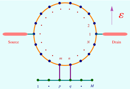
Figure 11: (Color online). A different bridge configuration compared to Fig. 1, where MQR is directly coupled to source and drain electrodes. The setup within the electrodes remains unaltered as considered in Fig. 1.

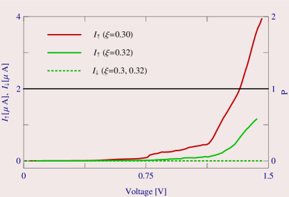
Figure 12: (Color online). Voltage dependence of up ($I_{\uparrow}$, left axis) and down ($I_{\downarrow}$, left axis) spin currents together with spin polarization coefficient ($P$, right axis) for different values of $\xi$ considering $E_{F}=-1.75$ eV for the setup given in Fig. 11. Here we choose $N=42$, $M=20$, $m=32$, $n=33$, $p=10$, $q=11$ and $\lambda=1$ eV.

considering two other different bridge setups with respect to Fig. 1. They are schematically shown in Figs. 11 and 14, respectively. In one case, the source and drain are attached to the MQR (see Fig. 11), instead of the MQW, and within these electrodes the setup remains unchanged as taken in Fig. 1. While, in the other case only the MQR is taken into account within the electrodes (see Fig. 14) to form a simple two-terminal bridge setup. Now we describe the results for these setups one by one.

In Figs. 12 and 13 the variation of spin dependent currents ($I_{\uparrow}$ and $I_{\downarrow}$) along with spin polarization coefficient $P$ as a function of applied bias voltage $V$ are shown for two distinct values of the field strength $\xi$. Focusing on the characteristics presented in the spectra

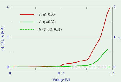
Figure 13: (Color online). Voltage dependence of up ($I_{\uparrow}$, left axis) and down ($I_{\downarrow}$, left axis) spin currents along with spin polarization coefficient ($P$, right axis) for different values of $\xi$ taking $E_{F}=1.75$ eV for the identical setup considered in Fig. 12. The parameters are same as taken in Fig. 12.

(Figs. 12 and 13), two observations are noteworthy. First, the current amplitudes for non-zero fields are too small compared to the current obtained in the model Fig. 1. Second, even for a slight increment of field strength $\xi$ current amplitude reduces very sharply, unlike the initial configuration i.e., Fig. 1 where current amplitude

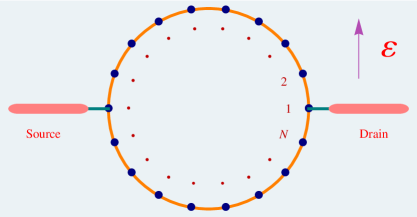
Figure 14: (Color online). Another setup where MQR is no longer coupled to MQW like the previous two bridges. The ring, subjected to an electric field, is directly coupled to two NM electrodes.

gets increased with increasing $\xi$. These features can be explained as follows. As stated, the MQR behaves like a correlated disordered system in presence of non-zero field $\xi$ since $\epsilon_{i}^{r}$’s are now field dependent, and therefore, the combined system can be regarded as an ordered-disordered coupled system. Thus, in the bridge given in Fig. 11, an electron which is coming from the source gets injected into the disordered region (MQR) and after traversing throughout the material (MQR and MQW) it eventually leaves from the disordered part (MQR) to enter into the drain. The width of disorderness becomes wider with the field strength $\xi$ and hence the energy levels associated with the MQR become more localized which lead to the reduced current across the junction. Comparing the results shown in Figs. 12 and 13, it is observed that the current amplitude decreases significantly even for a small increment of $\xi$ (from $0.3$ to $0.32$), and if we increase $\xi$ further current practically disappears. This

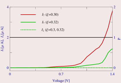
Figure 15: (Color online). $I_{\uparrow}$ (left axis), $I_{\downarrow}$ (left axis) and $P$ (right axis) as a function of voltage $V$ for different values of $\xi$ considering $N=42$, $\lambda=1$ eV and $E_{F}=-1.75$ eV for the setup given in Fig. 14.

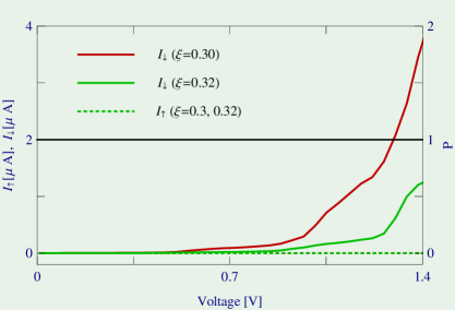
Figure 16: (Color online). $I_{\uparrow}$ (left axis), $I_{\downarrow}$ (left axis) and $P$ (right axis) as a function of voltage $V$ for different values of $\xi$ considering $N=42$, $\lambda=1$ eV and $E_{F}=1.75$ eV for the identical setup as taken in Fig. 15.

scenario is exactly opposite what we get in our previous geometry. In that model (Fig. 1) the ordered region (MQW) gradually decouples from the localized region (MQR) with increasing $\xi$ and the probability of traversing electrons through the ring also decreases which leads to enhanced spin current. Thus, by tuning $\xi$ we eventually enhance the probability of traversing electron through the wire which results larger current in the junction (Fig. 1), which is no longer possible if the electrodes are coupled directly to the ring (Fig. 11) instead of the wire as clearly seen from our results given in Figs. 12 and 13.

The existence of MQW does not provide any new significant behavior on spin dependent currents when the electrodes are coupled to the MQR, since for such a configuration electrons are eventually entering into the drain from a correlated disordered region for non-zero $\xi$. To corroborate this fact, in Figs. 15 and 16 we present the behavior of spin dependent currents including spin polarization coefficient for the junction configuration given in Fig. 14, where the ring is not attached to any MQW. Comparing the results of Figs. 12, 13, 15 and 16, we predict that the current-voltage characteristics show very less sensitivity on the MQW when the electrodes are coupled to the MQR. Thus, in short, we can emphasize that to design a tailor made spin based quantum device the proposed quantum system given in Fig. 1 is the most suitable one.

IV Concluding remarks

To conclude, in the present work we address a new approach of getting spin selective transmission through a non-magnetic – magnetic – non-magnetic bridge system based on Green’s function formalism. The magnetic system consists of a quantum ring which is directly coupled to a quantum wire and subjected to an in-plane electric field. From our results we find that the transmission spectrum gets significantly influenced by the electric field which directly reflects the current-voltage characteristics. Tuning the Fermi energy to a suitable energy zone a high degree of spin polarization ($\sim 100\%$) can also be achieved for a wide range of bias voltage for this setup. Our theoretical analysis promotes practical applications of externally controlled spin polarized quantum devices.

All the results presented in this communication are worked out at absolute zero temperature though its finite temperature extension is quite trivial. But, the thing is that at finite (low) temperatures no new phenomenon will appear since the thermal broadening of energy levels is too weak compared to the energy level broadening caused by the coupling of the bridging conductor to the side attached electrodes datta1 ; datta2 .

Before we end, it should be noted that to investigate spin selective transfer through this two-terminal geometry we compute all the numerical results considering some typical values of the physical parameters. But, all the physical phenomena studied here remain absolutely invariant for any other choices of the physical parameters describing the system. These features certainly demand the robustness of our analysis and give us confidence to propose an experiment in this line.

References

- (1) S. A. Wolf, D. D. Awschalom, R. A. Buhrman, J. M. Daughton, S. von Molnár, M. L. Roukes, A. Y. Chtchelkanova, and D. M. Treger, Science 294, 1488 (2001).
- (2) G. Prinz, Science 282, 1660 (1998).
- (3) G. Prinz, Phys. Today 48, 58 (1995).
- (4) J. Chen, M. A. Reed, A. M. Rawlett, and J. M. Tour, Science 286, 1550 (1999).
- (5) P. Ball, Nature (London) 404, 918 (2000).
- (6) L. P. Rokhinson, V. Larkina, Y. B. Lyanda-Geller, L. N. Pfeiffer, and K. W. West, Phys. Rev. Lett. 93, 146601 (2004).
- (7) S. Sahoo, T. Kontos, J. Furer, C. Hoffmann, M. Gräber, A. Cottet, and C. Schönenberger, Nature Phys. 1, 99 (2005).
- (8) N. Tombros, C. Jozsa, M. Popinciuc, H. T. Jonkman, and B. J. van Wees, Nature 448, 571 (2007).
- (9) M. N. Baibich, J. M. Broto, A. Fert, F. N. Van Dau, F. Petroff, P. Etienne, G. Creuzet, A. Friederich, and J. Chazelas, Phys. Rev. Lett. 61, 2472 (1998).
- (10) B. E. Kane, Nature (London) 393, 133 (1998).
- (11) V. Privman, I. D. Vagner, and G. Kventsel, Phys. Lett. A 239, 141 (1998).
- (12) G. Burkard, D. Loss, and D. P. DiVincenzo, Phys. Rev. B 59, 2070 (1999).
- (13) Yu. V. Pershin, I. D. Vagner, and P. Wyder, J. Phys.: Condens. Matter 15, 997 (2003).
- (14) J. Stöhr and H. C. Siegmann, Magnetism – From Fundamental to Nanoscale Dynamics (Springer, 2006).
- (15) S. Maekawa and T. Shinjo, Spin Dependent Transport in Magnetic Nanostructures, (CRC Press, 2002).
- (16) H. Yin, T. Lü, X. Liu, and H. Xue, Phys. Lett. A 285, 373 (2009).
- (17) F. Chi and S. Li, J. Appl. Phys. 100, 113703 (2006).
- (18) M. Dey, S. K. Maiti, and S. N. Karmakar, Phys. Lett. A 374, 1522 (2010).
- (19) M. W. Wu, J. Zhou, and Q. W. Shi, Appl. Phys. Lett. 6, 85 (2004).
- (20) M. Dey, S. K. Maiti, and S. N. Karmakar, J. Comput. Theor. Nanosci. 8, 253 (2011).
- (21) A. A. Shokri, M. Mardaani, and K. Esfarjani, Physica E 27, 325 (2005).
- (22) A. D. Güclü, P. Potasz, and P. Hawrylak, Phys. Rev. B 84, 035425 (2011).
- (23) O. Voznyy, A. D. Güclü, P. Potasz, and P. Hawrylak, Phys. Rev. B 83, 165417 (2011).
- (24) M. Modarresi, M. R. Roknabadi, and N. Shahtahmasebi, J. Magn. Magn. Mater. 350, 6 (2014).
- (25) K. Szalowski, J. Magn. Magn. Mater. 382, 318 (2015).
- (26) M. Lee and C. Bruder, Phys. Rev. B 73, 085315 (2006).
- (27) J. H. Ojeda, M. Pacheco, and P. A. Orellana, Nanotechnology 20, 434013 (2009).
- (28) M. Dey, S. K. Maiti, and S. N. Karmakar, Eur. Phys. J. B 80, 105 (2011).
- (29) K. Chang and F. M. Peeters, Solid State Commun. 120, 181 (2001).
- (30) A. A. Shokri and M. Mardaani, Solid State Commun. 137, 53 (2006).
- (31) D. Jin, Z. Li, M. Xiao, G. Jin, and A. Hu, J. Appl. Phys. 99, 08T304 (2004).
- (32) W. Long, Q.-F. Sun, H. Guo, and J. Wang, Appl. Phys. Lett. 83, 1397 (2003).
- (33) P. Zhang, Q. K. Xue, and X. C. Xie, Phys. Rev. Lett. 91, 196602 (2003).
- (34) Q.-F. Sun and X. C. Xie, Phys. Rev. B 91, 235301 (2006).
- (35) Q.-F. Sun and X. C. Xie, Phys. Rev. B 71, 155321 (2005).
- (36) F. Chi, J. Zheng, and L. L. Sun, Appl. Phys. Lett. 92, 172104 (2008).
- (37) T. P. Pareek, Phys. Rev. Lett. 92, 076601 (2004).
- (38) W. J. Gong, Y. S. Zheng, and T. Q. Lü, Appl. Phys. Lett. 92, 042104 (2008).
- (39) H. F. Lü and Y. Guo, Appl. Phys. Lett. 91, 092128 (2007).
- (40) Y. A. Bychkov and E. I. Rashba, JETP Lett. 39, 78 (1984).
- (41) G. Dresselhaus, Phys. Rev. 100, 580 (1955).
- (42) R. Winkler, Spin-orbit coupling effects in two-dimensional electron and hole Systems (Springer, 2003).
- (43) S. K. Maiti, S. Sil, and A. Chakrabarti, Phys. Lett. A 376, 2147 (2012).
- (44) G. Engels, J. Lange, Th. Schäpers, and H. Lüth, Phys. Rev. B 55, R1958 (1997).
- (45) L. Meier, G. Salis, I. Shorubalko, E. Gini, S. Schön, and K. Ensslin, Nature Physics 3, 650 (2007).
- (46) J. Premper, M. Trautmann, J. Henk, and P. Bruno, Phys. Rev. B 76, 073310 (2007).
- (47) C.-M. Hu, J. Nitta, T. Akazaki, H. Takayanagi, J. Osaka, P. Pfeffer, and W. Zawadzki, Phys. Rev. B 60, 7736 (1999).
- (48) D. Grundler, Phys. Rev. Lett. 84, 6074 (2000).
- (49) P. Földi, O. Kálmán, M. G. Benedict, and F. M. Peeters, Phys. Rev. B 73, 155325 (2006).
- (50) A. A. Kislev and K. W. Kim, J. App. Phys. 94, 4001 (2003).
- (51) S. Souma and B. K. Nikolić, Phys. Rev. B 70, 195346 (2004).
- (52) B. K. Nikolić and S. Souma, Phys. Rev. B 71, 195328 (2005).
- (53) M. Dey, S. K. Maiti, S. Sil, and S. N. Karmakar, J. Appl. Phys. 114, 164318 (2013).
- (54) S. K. Maiti, Phys. Lett. A 379, 361 (2015).
- (55) G. Cohen, O. Hod, and E. Rabani, Phys. Rev. B 76, 235120 (2007).
- (56) M. Dey, S. K. Maiti, and S. N. Karmakar, J. Appl. Phys. 109, 024304 (2011).
- (57) P. Orellana and F. Claro, Phys. Rev. Lett. 90, 178302 (2003).
- (58) G. Stefanucci, E. Perfetto, S. Bellucci, and M. Cini, Phys. Rev. B 79, 073406 (2009).
- (59) A.-M. Guo and Q.-F. Sun, Phys. Rev. Lett. 108, 218102 (2012).
- (60) P. A. Orellana, M. L. Ladrón de Guevara, M. Pacheco, and A. Latgé, Phys. Rev. B 68, 195321 (2003).
- (61) M. Modarresi, M. R. Roknabadi, and N. Shahtahmassebi, Physica B 415, 62 (2013).
- (62) M. Modarresi, M. R. Roknabadi, N. Shahtahmassebi, D. Vahedi, and H. Arabshahi, Physica E 43, 402 (2010).
- (63) S. K. Maiti, Phys. Lett. A 366, 114 (2007).
- (64) S. Sil, S. K. Maiti, and A. Chakrabarti, Phys. Rev. Lett. 101, 076803 (2008).
- (65) S. Datta, Electronic transport in mesoscopic systems (Cambridge University Press, Cambridge, 1995).
- (66) S. Datta, Quantum transport: Atom to transistor (Cambridge University Press, Cambridge, 2005).
- (67) D. Rai and M. Galperin, Phys. Rev. B 86, 045420 (2012).
- (68) R. Naaman and D. H. Waldeck, J. Phys. Chem. Lett. 3, 2178 (2012).
- (69) M. Dey, S. K. Maiti, and S. N. Karmakar, Org. Electron. 12, 1017 (2011).
- (70) P. Dutta, S. K. Maiti, and S. N. Karmakar, Org. Electron. 11, 1120 (2010).