Curvature effect on spin polarization in a three-terminal geometry in presence of Rashba spin-orbit interaction

Abstract

The robust effect of curvature on spin polarization is reported in a three-terminal bridge system where the bridging material is subjected to Rashba spin-orbit interaction. The results are examined considering two different geometric configurations, ring- and linear-like, of the material which is coupled to one input and two output leads. Our results exhibit absolute zero spin polarization for the linear sample, while finite polarization is obtained in output leads for the ring-like sample.

I Introduction

The study of spin dependent transport in low-dimensional systems has been largely dominated in the last few decades due to the rapid advancement in nano-scale science and technology th1 ; th2 ; th3 ; th4 ; th5 ; th6 ; th7 ; th8 ; san1 ; san2 ; san3 ; san4 ; th9 ; th10 ; san10 ; ex1 ; ex2 ; ex3 . Controlling electron’s spin degree of freedom is extremely important for the development of quantum information processing as well as quantum computation wolf . The spin-orbit (SO) interaction which couples the electron’s spin to the charge degree of freedom provides a much deeper insight for generating spin current and also its manipulation intrinsic1 ; intrinsic2 ; intrinsic3 ; intrinsic4 ; intrinsic5 ; intrinsic6 rather than the usual methodologies wang ; xie . Earlier, people were mainly using wang ; xie ferromagnetic leads or external magnetic field to get spin filtering action though these are not very suitable especially for low-dimensional systems, since in one case a large resistivity mismatch is observed while in the other case the main difficulty appears for confining a huge magnetic field into a narrow region, like a nano-ring.

Depending on the sources, spin-orbit interaction is classified in two different categories: one is called extrinsic type which appears mainly due to magnetic impurities, while the other is defined as intrinsic type that appears as a result of lacking of inversion symmetry. In this category generally two kinds of spin-orbit interactions are taken into account. They are called as Rashba and Dresselhaus SO interactions rashba ; dressel ; winkler . The first one is associated with the inversion asymmetry of the structure and its strength can be regulated by means of external gate potential, and the second one is related to the bulk inversion asymmetry whose coupling strength depends on the material.

Considering the coupling of spin degree of freedom to the momentum of an electron, spin polarized currents in output terminals of a multi-terminal conductor can be achieved from a purely unpolarized electron beam injected to the input terminal mlt1 ; mlt2 ; mlt3 ; mlt4 ; mlt5 . The existing literature suggest that a lot of theoretical progress has already been done to explore spin selective transmission through different model geometries. For example, a planar T-shaped conductor mlt1 with a ring resonator exhibits polarized spin currents in outgoing leads in presence of Rashba SO interaction. In other work Peeters et al. have shown how a ring-like geometry can be utilized as an electron spin beam splitter exploring the possible quantum interference effect in presence of SO coupling mlt3 . At the same time Nikolic and his group mlt4 ; mlt5 put forward several key ideas in this particular field.

In spite of the considerable volume of work available in this particular area, a practically unexplored issue is how does the curvature of a material which is clamped within input and output leads influence spin polarization.

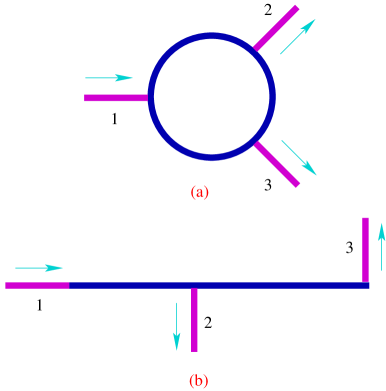
Figure 1: (Color online). Schematic diagram of a three-terminal bridge setup, where the arrows correspond to the movement of electrons through one input and two output terminals. Two different geometrical shapes, ring- and linear-like, of a particular sample subjected to Rashba SO interaction are taken into account to explore the curvature effect on spin polarization in multi-terminal system.

To the best of our knowledge, this part is unaddressed so far. In the present work we essentially focus towards this direction. We investigate the curvature effect on spin polarization by considering two simple geometries: a simple linear conductor and a ring-like geometry which is formed by bending the chain.

The results are quite interesting. Using a tight-binding (TB) framework and based on Green’s function formalism we show that for a ring shaped conductor spin polarized currents are obtained in output leads of a multi-terminal geometry from a completely unpolarized beam of electrons, while absolute zero spin polarization is obtained for the linear conductor.

The rest of the paper is organized as follows. Section II illustrates two different models together with a brief theoretical description to obtain spin polarization in two output leads. Section III contains numerical results and discussion, and finally, in Section IV we summarize our essential results.

II Model and theoretical framework

In this section we describe two different systems of our study and present a general theory for calculating spin polarization coefficient $P^{z}$ in two output leads based on Green’s function formalism.

II.1 Model and Hamiltonian

The three-terminal bridge setup is schematically shown in Fig. 1, where we take two different configurations of the same material. In one configuration we choose a finite one-dimensional ($1$D) chain, which is then bent to form a $1$D ring to generate another configuration. In both these two cases the material, subjected to Rashba spin-orbit interaction, is connected with one input (lead-1) and two output leads (lead-2 and lead-3).

A tight-binding framework is given under the nearest-neighbor hopping approximation to describe the bridging material (ring/chain) and the side-attached leads. The TB Hamiltonian of the entire system reads as,

$$H=H_{\mbox{\tiny sample}}+H_{\mbox{\tiny leads}}+H_{\mbox{\tiny tun}}$$ (1)

where three different terms in the right side correspond to the Hamiltonians of three different regions of the bridge system those are elaborately explained below.

The first term, $H_{\mbox{\tiny sample}}$, describes the Hamiltonian of the conductor placed between the incoming and outgoing leads. Depending on its geometry (ring-like or chain-like) the Hamiltonian looks different. For a $N$-site linear conductor subjected to Rashba SO interaction the TB Hamiltonian liu ; san9 gets the form:

$$H_{\mbox{\tiny sample}} = \sum_{n}\mbox{\boldmath$c$}_{n}^{{\dagger}}\mbox{\boldmath$\epsilon$}\mbox{\boldmath$c$}_{n}+\sum_{n}\left(\mbox{\boldmath$c$}_{n}^{{\dagger}}\mbox{\boldmath$t$}\mbox{\boldmath$c$}_{n+1}+h.c.\right)$$ (2)

$$+\sum_{n}\left(i\,t_{\mbox{\small so}}\mbox{\boldmath$c$}_{n}^{{\dagger}}[\vec{\sigma}\times\hat{d}_{n,n+1}]_{z}\mbox{\boldmath$c$}_{n+1}+h.c.\right)$$

where,
$\mbox{\boldmath$c$}^{\dagger}_{n}=\left(\begin{array}[]{cc}c_{n\uparrow}^{\dagger}&c_{n\downarrow}^{\dagger}\end{array}\right);$ $\mbox{\boldmath$c$}_{n}=\left(\begin{array}[]{c}c_{n\uparrow}\\ c_{n\downarrow}\end{array}\right);$ $\mbox{\boldmath$\epsilon$}=\left(\begin{array}[]{cc}\epsilon&0\\ 0&\epsilon\end{array}\right)$ and
$\mbox{\boldmath$t$}=t\left(\begin{array}[]{cc}1&0\\ 0&1\end{array}\right).$
 
In the above expression, $\mbox{\boldmath$c$}_{n\sigma}^{\dagger}$ and $\mbox{\boldmath$c$}_{n\sigma}$ are the creation and annihilation operators, respectively, for an electron with spin $\sigma(\uparrow,\downarrow)$ at the $n$-th atomic site of the sample. $\epsilon$ is the on-site energy and $t$ measures the isotropic nearest-neighbor hopping integral. The parameter $t_{\mbox{\small so}}$ describes the Rashba SO coupling strength and the term $\vec{\sigma}$ gives the spin angular momentum of the electron. The unit vector $\hat{d}_{n,n+1}$ describes the direction of the movement of an electron between the sites $n$ and $n+1$.

When this $N$-site linear conductor is bent to form a ring the Hamiltonian becomes san5 ; san6 ; san7 ; san8 ,

$$H_{\mbox{\tiny sample}} = \sum_{i}\mbox{\boldmath$c$}_{n}^{{\dagger}}\mbox{\boldmath$\epsilon$}\mbox{\boldmath$c$}_{n}+\sum_{n}\left(\mbox{\boldmath$c$}_{n}^{{\dagger}}\mbox{\boldmath$t$}\mbox{\boldmath$c$}_{n+1}+h.c.\right)$$ (3)

$$+\sum_{n}\left(\mbox{\boldmath$c$}_{n}^{{\dagger}}\mbox{\boldmath$t$}_{n,n+1}\mbox{\boldmath$c$}_{n+1}+h.c.\right)$$

where,
$\mbox{\boldmath$t$}_{n,n+1}=it_{\mbox{\small so}}\left\{\mbox{\boldmath$\sigma_{x}$}\cos\left(\frac{\varphi_{n}+\varphi_{n+1}}{2}\right)+\mbox{\boldmath$\sigma_{y}$}\sin\left(\frac{\varphi_{n}+\varphi_{n+1}}{2}\right)\right\}$ with $\varphi_{n}=2\pi(n-1)/N$. All the other symbols used in Eq. 3 carry their usual meanings.

In our theoretical framework, three metallic leads are considered to be identical, semi-infinite and free from any kind of impurities and spin-orbit interaction. We can express them as,

$$H_{\mbox{\tiny leads}}=\sum_{\alpha}H_{\alpha}$$ (4)

where $\alpha=1,2,3$ for the three leads. In the absence of any SO coupling $H_{\alpha}$ takes the form:

$$H_{\alpha}=\sum\limits_{i}\mbox{\boldmath$c$}_{i}^{\dagger}\mbox{\boldmath$\epsilon$}_{l}^{\alpha}\mbox{\boldmath$c$}_{i}+\sum_{i}\left(\mbox{\boldmath$c$}_{i}^{\dagger}\mbox{\boldmath$t$}_{l}^{\alpha}\mbox{\boldmath$c$}_{i+1}+h.c.\right)$$ (5)

with $\mbox{\boldmath$\epsilon$}_{l}^{\alpha}=\epsilon_{l}^{\alpha}\left(\begin{array}[]{cc}1&0\\ 0&1\end{array}\right)$ and $\mbox{\boldmath$t$}_{l}^{\alpha}=t_{l}^{\alpha}\left(\begin{array}[]{cc}1&0\\ 0&1\end{array}\right)$.
 
where $\epsilon_{l}^{\alpha}$ and $t_{l}^{\alpha}$ are the site energy and nearest-neighbor hopping integral, respectively, in the $\alpha$-th lead. Other factors carry their usual meanings as stated earlier. Out of these three leads, lead-1 is treated as the input terminal, while the other two are considered as the output terminals and all of them are coupled to the conductor through the hopping integral $t_{c}$. Here we assume that the lead-1 is always attached to site $1$ and the other two leads are coupled to the sites $p$ and $q$, those are variables, of the conductor. Following the same footing as above, we can write the TB Hamiltonian to describe the conductor-to-lead coupling as,

$$H_{\mbox{\tiny tun}}=\sum_{\alpha}H_{{\mbox{\tiny tun}},\alpha}.$$ (6)

Here,

$$H_{{\mbox{\tiny tun}},\alpha}=\left[\mbox{\boldmath$c$}^{\dagger}_{i}\mbox{\boldmath$t$}_{c}\mbox{\boldmath$c$}_{n}+\mbox{\boldmath$c$}^{\dagger}_{n}\mbox{\boldmath$t$}_{c}\mbox{\boldmath$c$}_{i}\right]$$ (7)

with $\mbox{\boldmath$t$}_{c}=t_{c}\left(\begin{array}[]{cc}1&0\\ 0&1\end{array}\right).$
The site $i$ corresponds to the boundary site of the lead, and it is coupled to the $n$-th site of the conductor, which is variable.

II.2 Evaluation of polarization coefficient $P^{z}$ in terms of transmission probabilities

The spin polarization coefficient in the output leads is defined as san2 ; pola1 ; pola2 ; pola3 ,

$$P^{z}=\frac{T_{\uparrow\uparrow}+T_{\downarrow\uparrow}-T_{\uparrow\downarrow}-T_{\downarrow\downarrow}}{T_{\uparrow\uparrow}+T_{\downarrow\uparrow}+T_{\uparrow\downarrow}+T_{\downarrow\downarrow}}$$ (8)

where, $T_{\sigma\sigma^{\prime}}$ gives the transmission probability of an injecting electron with spin $\sigma$ which gets transmitted through the drain with spin $\sigma^{\prime}$. When $\sigma=\sigma^{\prime}$ we get pure spin transmission, while for the other case spin flip transmission is obtained. Equation 8 is the general expression of spin polarization coefficient between any two leads $i$ and $j$, and, for our three-terminal system we call the polarization coefficients in two outgoing leads as $P_{1}^{z}$ and $P_{2}^{z}$. In the present approach we select the quantization direction along the $Z$ axis for simplification.

To calculate transmission coefficient $T_{\sigma\sigma^{\prime}}$ we use Green’s function formalism datta1 ; datta2 . In this framework the two-terminal transmission probability between the leads $i$ and $j$ is defined as $T_{\sigma\sigma^{\prime}}=\mbox{Tr}\left[\Gamma_{i}^{\sigma}G_{c}^{r}\Gamma_{j}^{\sigma^{\prime}}G_{c}^{a}\right]$. Here $G_{c}^{r}$ and $G_{c}^{a}$ are the retarded and advanced Green’s functions, respectively, of the sample considering the effects of the electrodes. $G_{c}^{r}=\left(E-H_{\mbox{\tiny sample}}-\sum\limits_{\sigma}\Sigma_{1}^{\sigma}-\sum\limits_{\sigma}\Sigma_{2}^{\sigma}-\sum\limits_{\sigma}\Sigma_{3}^{\sigma}\right)^{-1}$, where $E$ is the energy of an injecting electron, and $\Sigma_{i}^{\sigma}$’s ($i=1,2,3$) are the self-energies due to coupling of the conductor to the leads and $\Gamma_{i}^{\sigma}$’s are their imaginary parts. In Refs. datta1 ; datta2 the detailed calculations of self-energy matrices are available.

III Numerical results and discussion

Based on the above theoretical framework we now analyze our numerical results. Throughout the analysis we fix the electronic temperature of the system to absolute zero, and for simplification, we put $c=e=h=1$. Other common parameters are as follows: $\epsilon=\epsilon_{l}^{\alpha}=0$ and $t=t_{l}^{\alpha}=t_{c}=1$. The Rashba SO coupling strength $t_{\mbox{\small so}}$ and all the energy scales are measured in unit of the hopping integral $t$.

Before focusing to the central point i.e., the curvature effect on spin polarization in a multi-terminal (more than one output lead) system in presence of Rashba SO interaction, we want to have a short glimpse on the system where a conductor subjected to SO interaction is coupled to a single input and a single output lead i.e., a two-terminal system. Following our extensive numerical calculations we can conclude that irrespective of the curvature of the bridging material, only SO interaction cannot induce spin polarization in output lead of a two-terminal system. We verify it considering different geometrical shapes of the conductor, e.g., circle, square, triangle, polygon, linear, etc. In few recent works mlt1 ; moo it has also been shown that only SO interaction

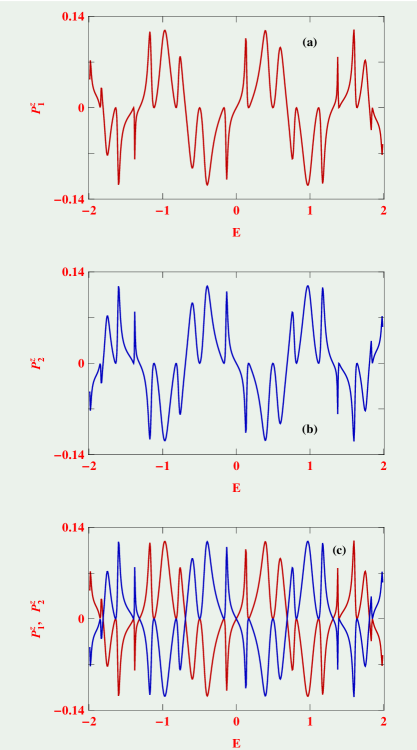
Figure 2: (Color online). Energy dependence of spin polarization coefficients $P_{1}^{z}$ and $P_{2}^{z}$ in two output leads, in (a) and (b) respectively, for a three-terminal mesoscopic ring when the output leads are attached symmetrically with respect to the input lead. These coefficients ($P_{1}^{z}$ and $P_{2}^{z}$) are superposed with each other in (c) for comparison. The parameters are: $N=52$, $t_{\mbox{\small so}}=0.5$, $p=22$ and $q=32$.

is incapable of producing spin polarization. The reason is that, in presence of SO coupling the time-reversal symmetry is still preserved, and therefore, it doesn’t break the Kramer’s degeneracy between the $|k\uparrow\rangle$ and $|-k\downarrow\rangle$ states which results vanishing spin current in the output lead of a two-terminal system. The degeneracy gets removed when the system is subjected to any kind of magnetic impurity or external magnetic field. Under this situation a two-terminal system with SO coupling exhibits polarized spin currents san2 . This phenomenon has already been established in the literature, but the essential issue of our present analysis – the interplay between the curvature of the material and the multi-leads has not been addressed earlier.

To explore it, in Fig. 2 we present the results for a three-terminal mesoscopic ring considering $N=52$ and $t_{\mbox{\small so}}=0.5$. Here, the two outgoing leads are attached

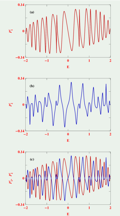
Figure 3: (Color online). Energy dependence of spin polarization coefficients $P_{1}^{z}$ and $P_{2}^{z}$ in two output leads, in (a) and (b) respectively, for a three-terminal mesoscopic ring when the output leads are attached asymmetrically with respect to the source lead. These coefficients ($P_{1}^{z}$ and $P_{2}^{z}$) are superposed with each other in (c) for comparison. The parameters are: $N=52$, $t_{\mbox{\small so}}=0.5$, $p=27$ and $q=39$.

symmetrically ($p=22$ and $q=32$) with respect to the incoming lead, as shown schematically in Fig. 1(a). The upper panel of Fig. 2 corresponds to the energy dependence of spin polarization coefficient for the one output lead, while for the other output terminal it is shown in the middle panel of Fig. 2, and, finally they are placed together in the lower panel of this figure to compare the polarization coefficients properly. From these spectra it is observed that finite spin polarizations, associated with the energy eigenvalues of the ring subjected to only SO interaction, are obtained in both the two outgoing leads though the system is free from any kind of magnetic impurities. Most interestingly, we also see that the coefficients $P_{1}^{z}$ and $P_{2}^{z}$ are exactly identical in magnitude and opposite in sign for each value of the incident electron energy $E$. This phenomenon can be explained as follows. The spin polarization

Figure 4: (Color online). Energy dependence of spin polarization coefficients $P_{1}^{z}$ and $P_{2}^{z}$ in a three-terminal mesoscopic chain considering $N=52$ and $t_{\mbox{\small so}}=0.5$ for two different chain-to-lead interface geometries, where (a) $p=26$, $q=52$ and (b) $p=20$, $q=40$.

coefficient $P^{z}$ describes the normalized difference among the up and down spin charge currents propagating through the outgoing leads, since in our present scheme we assume the quantized direction along the Z direction. In a multi-lead geometry i.e., when more than one outgoing lead is coupled to the system the Kramer’s degeneracy between the $|k\uparrow\rangle$ and $|-k\downarrow\rangle$ gets removed and depending on the allowed paths of the moving electrons spin dependent scattering takes place. The spin dependent force associated with the SO coupling is responsible for this scattering. Now, in the ring-like geometry electrons can go through two different paths, and accordingly, the up and down spin electrons get deflected in two opposite directions by the spin dependent force during the movement of electrons through the ring geometry in presence of SO interaction which results spin selective transmission through the outgoing leads. This is the key aspect of observing mesoscopic spin Hall effect san9 and the accumulation of opposite spin electrons on the opposite edges of a finite width conductor. Since the two outgoing leads are coupled symmetrically to the ring geometry with respect to the incoming lead, $P_{1}^{z}$ and $P_{2}^{z}$ get equal magnitude. Their sign reversals are also understood from Eq. 8.

By breaking the ring-lead interface geometry one can achieve spin polarizations with unequal magnitudes. The results are shown in Fig. 3 when the output leads are attached asymmetrically with respect to the source lead. Here we fix $p=27$ and $q=39$, and all the other parameters are kept identical as set in Fig. 2. It is clearly seen that, unlike the symmetric configuration, the magnitudes of $P^{z}$ in two output leads are no longer equal for the asymmetrically connected ring-lead bridge setup. This is exclusively due to the quantum interference effect among the electronic waves propagating through different arms of the ring geometry. Apart from getting unequal magnitudes of polarization coefficients in two output leads, all the other properties remain exactly invariant as described earlier in the case of symmetric configuration.

From these results we can emphasize that, for the three-terminal ring geometry we get spin polarization due to SO interaction only, since the sample is free from any kind of magnetic impurity or external magnetic field, but a two-terminal ring geometry cannot provide polarize spin current under this situation. Here, it is important to note that although the Kramer’s degeneracy between the $|k\uparrow\rangle$ and $|-k\downarrow\rangle$ gets removed by coupling the conductor with a third lead or more, but it doesn’t ensure to get non-vanishing spin polarization in output leads which can be clearly understood from the following discussion.

The scenario becomes highly significant when the ring-like sample is transformed into the linear-like one. The results are shown in Fig. 4 considering two different chain-to-lead interface geometries. In one configuration (Fig. 4(a)) the outgoing leads are coupled to the sites $26$ and $52$ of the linear conductor, while these coupling sites are $20$ and $40$ for the other configuration (Fig. 4(b)). The total number of atomic sites $N$ and the Rashba SO coupling are kept unchanged as taken in Fig. 2. From the spectra presented in Fig. 4, we interestingly see that both $P_{1}^{z}$ and $P_{2}^{z}$ drop exactly to zero for the entire energy band spectrum, and, these results are independent of the chain-to-lead interface geometry as well as the strength of the SO coupling, which we confirm through our considerable numerical work. This is really appealing in the sense that a same material subjected to SO coupling exhibits finite spin polarization for one geometrical shape, while absolute zero spin polarization is obtained in the other geometrical configuration for a multi-terminal bridge setup. This is solely due to the effect of curvature. For the linear chain the up and down spin electrons can propagate only in a particular direction. Either it can be along X or Y direction depending on the choice of the co-ordinate system. Under this situation, the spin dependent force which essentially scatter opposite spin electrons becomes zero, and therefore, no spin polarization is available even though the Kramer’s degeneracy is broken for such a multi-terminal bridge setup. The disappearance of such spin dependent force in a linear sample can be justified from the following analysis. For a linear chain the Rashba dependent Hamiltonian in the continuum model representation gets the form xu : $(t_{\mbox{\small so}}/\hbar)\sigma_{y}p_{x}$, assuming the movement of electrons along the X direction. Considering this Hamiltonian if we calculate $\ddot{x}$, $x$ being the position operator, then the output becomes exactly zero which immediately suggests vanishing spin dependent force since the force is directly proportional to $\ddot{x}$. To get a finite spin

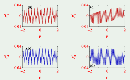
Figure 5: (Color online). Energy dependence of spin polarization coefficients $P_{1}^{z}$ and $P_{2}^{z}$ in a three-terminal mesoscopic ring for two distinct ring-to-lead interface geometries considering $N=200$ and $t_{\mbox{\small so}}=0.5$. The results for the symmetric configuration are presented in the first column where we set $p=82$ and $q=120$, while in the second column they are shown for the asymmetric configuration setting $p=101$ and $q=151$.

dependent force both the components $p_{x}$ and $p_{y}$ are needed in the Rashba term which is not possible in the case of a linear chain. Therefore, spin dependent scattering is no longer available, even in the presence of multi-leads. Now, an important point which should be noted here that when a linear conductor is properly bent to form a regular ring shaped geometry, the SO coupling strength may be affected due to its curvature, but that doesn’t at all change the present physical scenario, and therefore, we consider the identical coupling strength for both these two geometrical configurations for the sake of simplification in our model calculations.

The results presented so far to explore the curvature effect on spin polarization in a three terminal geometry are computed for a conductor with only $52$ sites. Keeping in mind a possible experimental realization one may think how such a small sized conductor can be used to design a conductor-lead bridge setup. To establish this fact now we present the spin polarization coefficients $P_{1}^{z}$ and $P_{2}^{z}$ taking a $200$-site conductor for its two different shapes as considered earlier i.e., ring-like and the linear-like one. For the ring-like geometry, the results are presented in Fig. 5, whereas for the other case they are shown in Fig. 6, and for both these two cases the results are computed for two distinct electrode-to-conductor configurations (symmetric and asymmetric) to justify the robustness of our investigation. From the spectra given in Fig. 5 it is observed that, like Fig. 2, here also the polarization coefficients $P_{1}^{z}$ and $P_{2}^{z}$ become exactly identical in magnitude and opposite in sign (1st column of Fig. 5) when the ring is attached symmetrically to

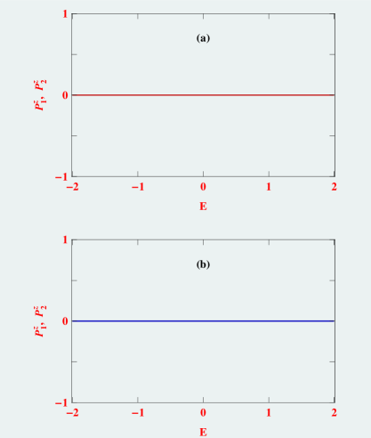
Figure 6: (Color online). Energy dependence of spin polarization coefficients $P_{1}^{z}$ and $P_{2}^{z}$ in a three-terminal mesoscopic chain considering $N=200$ and $t_{\mbox{\small so}}=0.5$ for two different chain-to-lead interface geometries, where (a) $p=100$, $q=200$ and (b) $p=50$, $q=150$.

the outgoing leads. These coefficients $P_{1}^{z}$ and $P_{2}^{z}$ are no longer identical in magnitude for the asymmetric ring-lead configuration (2nd column of Fig. 5), as expected. This is exactly what we get in a $52$-site ring as shown in Fig. 3. For the linear-shaped conductor with $N=200$ a vanishing spin polarization is obtained (Fig. 6) in its output leads for the entire energy band region irrespective of the chain-to-lead interface geometry and it is exactly similar in nature which we get earlier in the case of a $52$-site chain (Fig. 4). From these results we can emphasize that apart from getting more peaks and dips in $P^{z}$-$E$ spectrum for the ring-shaped conductor with increasing $N$, all the basic physical properties i.e., non-vanishing spin polarization coefficients with equal and/or unequal magnitudes associated with the ring-lead interface geometry and absolute zero spin polarization in the linear-like conductor irrespective of its coupling configuration to side-attached leads remain exactly unchanged. For a very large sized ring several peaks and dips appear in $P^{z}$-$E$ spectrum from which it may seem that the spectrum is quasi-continuous, but looking it carefully one can always find distinct peaks since $N$ is finite. Thus, our essential goal of getting finite and vanishing spin polarizations in a multi-terminal geometry constructed with the same material with different curvatures is established.

IV Conclusion

To summarize, in the present communication we establish the curvature effect on Rashba spin-orbit interaction induced spin polarization in a three-terminal bridge setup within a tight-binding framework based on Green’s function formalism. The results are analyzed considering two different shaped geometries of the same material. In one configuration we select the bridging material in a linear-like, which is then bent to form a ring-like geometry. Quite interestingly, we find that finite polarization is obtained in two output leads for ring shaped geometry, while absolute zero spin polarization is noticed when the sample becomes linear. This phenomenon also holds true even for any other higher-terminal bridge setup and independent of the lead-conductor interface geometries.

In addition to this ring-like geometry one might expect finite spin polarization in output leads for other geometrical configurations, except the linear one, which essentially leads to the robust effect of curvature on spin polarization in a multi-terminal bridge system.

All the results described in this communication are worked out at absolute zero temperature, though the finite temperature extension of this analysis is extremely trivial. The thing is that at finite temperature no new phenomenon will appear and all the physical pictures presented here remain unaltered even at finite (low) temperature since the broadening of energy levels of the conductor due to its coupling with the side-attached leads is too large compared to the thermal broadening datta1 ; datta2 ; san11 ; san12 ; san13 .

In the present work, we ignore the effect of on-site electron-electron (e-e) interaction. We can incorporate this effect in our formalism in different ways. One possible route is the mean field approximation ee1 ; ee2 ; ee3 ; ee4 ; ee5 . But, for this particular study e-e interaction doesn’t provide any such new insight since it cannot scatter up and down spin electrons in opposite edges of the sample, as spin-orbit interaction does. Only some modifications in magnitudes of $P_{1}^{z}$ and $P_{2}^{z}$ can be expected.

Before we end, it should be noted that to explore the effect of curvature on spin polarization in a three-terminal bridge setup we compute our numerical results considering some typical values of the parameters describing the systems. But, all these physical properties i.e., vanishing spin polarization in output leads of a linear-like conductor and finite spin polarization for a ring-like geometry remain absolute unchanged for any other set of parameter values. These features certainly demand an experiment in this line.

References

- (1) I. A. Shelykh, N. T. Bagraev, N. G. Galkin, and L. E. Klyanchkin, Phys. Rev. B 71, 113311 (2005).
- (2) H. W. Wu, J. Zhou, and Q. W. Shi, Appl. Phys. Lett. 85, 1012 (2004).
- (3) D. Frustaglia, M. Hentschel, and K. Richter, Phys. Rev. Lett. 87, 256602 (2001).
- (4) R. Ionicioiu and I. D’Amico, Phys. Rev. B 67, 041307(R) (2003).
- (5) A. A. Shokri, M. Mardaani, and K. Esfarjani, Physica E 27, 325 (2005).
- (6) M. Mardaani and A. A. Shokri, Chem. Phys. 324, 541 (2006).
- (7) A. A. Shokri and A. Daemi, Eur. Phys. J. B 69, 245 (2009).
- (8) A. A. Shokri and A. Saffarzadeh, J. Phys.: Condens. Matter 16, 4455 (2004).
- (9) M. Dey, S. K. Maiti, and S. N. Karmakar, Eur. Phys. J. B 80, 105 (2011).
- (10) M. Dey, S. K. Maiti, and S. N. Karmakar, J. Appl. Phys. 109, 024304 (2011).
- (11) M. Dey, S. K. Maiti, and S. N. Karmakar, Phys. Lett. A 374, 1522 (2010).
- (12) M. Dey, S. K. Maiti, and S. N. Karmakar, J. Comput. Theor. Nanosci. 8, 253 (2011).
- (13) S. Bellucci and P. Onorato, Phys. Rev. B 78, 235312 (2008).
- (14) S. Bellucci and P. Onorato, J. Phys.: Condens. Matter 19, 395020 (2007).
- (15) M. Dey, S. K. Maiti, S. Sil, and S. N. Karmakar, J. Appl. Phys. 114, 164318 (2013).
- (16) L. P. Rokhinson, V. Larkina, Y. B. Lyanda-Geller, L. N. Pfeiffer, and K. W. West, Phys. Rev. Lett. 93, 146601 (2004).
- (17) S. Sahoo, T. Kontos, J. Furer, C. Hoffmann, M. Gräber, A. Cottet, and C. Schönenberger, Nature Phys. 1, 99 (2005).
- (18) N. Tombros, C. Jozsa, M. Popinciuc, H. T. Jonkman, and B. J. van Wees, Nature 448, 571 (2007).
- (19) S. A. Wolf, D. D. Awschalom, R. A. Buhrman, J. M. Daughton, S. von Molnár, M. L. Roukes, A. Y. Chtchelkanova, and D. M. Treger, Science 294, 1488 (2001).
- (20) Q.-F. Sun and X. C. Xie, Phys. Rev. B 73, 235301 (2006).
- (21) Q.-F. Sun and X. C. Xie, Phys. Rev. B 71, 155321 (2005).
- (22) F. Chi, J. Zheng, and L. L. Sun, Appl. Phys. Lett. 92, 172104 (2008).
- (23) T. P. Pareek, Phys. Rev. Lett. 92, 076601 (2004).
- (24) W. Gong, Y. Zheng, and T. Lü, Appl. Phys. Lett. 92, 042104 (2008).
- (25) H. F. Lü and Y. Guo, Appl. Phys. Lett. 91, 092128 (2007).
- (26) W. Long, Q.-F. Sun, H. Guo, and J. Wang, Appl. Phys. Lett. 83, 1397 (2003).
- (27) P. Zhang, Q. K. Xue, and X. C. Xie, Phys. Rev. Lett. 91, 196602 (2003).
- (28) Y. A. Bychkov and E. I. Rashba, JETP Lett. 39, 78 (1984).
- (29) G. Dresselhaus, Phys. Rev. 100, 580 (1955).
- (30) R. Winkler, Spin-orbit coupling effects in two-dimensional electron and hole Systems (Springer, 2003).
- (31) A. A. Kislev and K. W. Kim, J. App. Phys. 94, 4001 (2003).
- (32) I. A. Shelykh, N. G. Galkin, and N. T. Bagraev, Phys. Rev. B 72, 235316 (2005).
- (33) P. Földi, O. Kálmán, M. G. Benedict, and F. M. Peeters, Phys. Rev. B 73, 155325 (2006).
- (34) S. Souma and B. K. Nikolić, Phys. Rev. B 70, 195346 (2004).
- (35) B. K. Nikolić and S. Souma, Phys. Rev. B 71, 195328 (2005).
- (36) G. Liu, P. Zhang, Z. Wang, and S.-S. Li, Phys. Rev. B 79, 035323 (2009).
- (37) M. Dey, S. K. Maiti, and S. N. Karmakar, J. Appl. Phys. 112, 024322 (2012).
- (38) S. K. Maiti, M. Dey, S. Sil, A. Chakrabarti, and S. N. Karmakar, Europhys. Lett. 95, 57008 (2011).
- (39) S. Sil, S. K. Maiti, and A. Chakrabarti, J. App. Phys. 112, 024321 (2012).
- (40) S. K. Maiti, S. Sil, and A. Chakrabarti, Phys. Lett. A 376, 2147 (2012).
- (41) S. K. Maiti, J. Appl. Phys. 110, 064306 (2011).
- (42) R. Gutierrez, E. Díaz, R. Naaman, and G. Cuniberti, Phys. Rev. B 85, 081404(R) (2012).
- (43) A.-M. Guo and Q.-F. Sun, Phys. Rev. B 86, 115441 (2012).
- (44) A.-M. Guo and Q.-F. Sun, Phys. Rev. Lett. 108, 218102 (2012).
- (45) S. Datta, Electronic transport in mesoscopic systems (Cambridge University Press, Cambridge, 1995).
- (46) S. Datta, Quantum transport: Atom to transistor (Cambridge University Press, Cambridge, 2005).
- (47) J. H. Bardarson and J. E. Moore, Rep. Prog. Phys. 76, 056501 (2013).
- (48) W. Xu and Y. Guo, Phys. Lett. A 340, 281 (2005).
- (49) M. Dey, S. K. Maiti, and S. N. Karmakar, Org. Electron. 12, 1017 (2011).
- (50) P. Dutta, S. K. Maiti, and S. N. Karmakar, Org. Electron. 11, 1120 (2010).
- (51) S. K. Maiti, Solid State Commun. 149, 1623 (2009).
- (52) S. K. Maiti and A. Chakrabarti, Phys. Rev. B 82, 184201 (2010).
- (53) H. Kato and D. Yoshioka, Phys. Rev. B 50, 4943 (1994).
- (54) A. Kambili, C. J. Lambert, and J. H. Jefferson, Phys. Rev. B 60, 7684 (1999).
- (55) S. K. Maiti, Solid State Commun. 150, 2212 (2010).
- (56) S. K. Maiti, Phys. Status Solidi B 248, 1933 (2011).