Abstract

We consider an optimal partition of resources (e.g. consumers) between several agents, given utility functions (”wisdoms”) for the agents and their capacities. This problem is a variant of optimal transport (Monge-Kantorovich) between two measure spaces where one of the measures is discrete (capacities) and the costs of transport are the wisdoms of the agents. We concentrate on the individual value for each agent under optimal partition and show that, counter-intuitively, this value may decrease if the agent’s wisdom is increased. Sufficient and necessary conditions for the monotonicity with respect to the wisdom functions of the individual values will be given, independently of the other agents. The sharpness of these conditions is also discussed.

Motivated by the above we define a cooperative game based on optimal partition and investigate conditions for stability of the grand coalition.

1 Introduction

Let $X$ be a set of ”consumers”. Let $I:=\{1,\ldots N\}$ be a set of ”agents”. For each agent $i\in I$ we associate a real valued function $\psi_{i}$ on $X$. This symbolizes the agent’s ”wisdom”: $\psi_{i}(x)$ is the profit that agent $i$ can make for a consumer $x$, if the latter uses her service. We denote the ”wisdom vector” $\vec{\psi}:=(\psi_{1},\ldots\psi_{N}):X\rightarrow\mathbb{R}^{N}_{+}$.

Let $\mu$ be the distribution of consumers in $X$. In particular $\mu(X)$ is the number of consumers.

Each agent $i$ has a limited capacity $M_{i}>0$. This symbolizes the total number of consumers she can serve. In other words, an agent $i$ can serve a measurable set $A_{i}\subset X$ of consumers for which $\mu(A_{i})\leq M_{i}$. Another assumption is that each consumer can hire at most one agent, meaning $\mu(A_{i}\cap A_{j})=0$ if $i\not=j$.

The profit made by an agent $i$ for her consumers $A_{i}$ is just

$$P_{\psi_{i}}(A_{i}):=\int_{A_{i}}\psi_{i}d\mu\ .$$

Let $\vec{M}:=(M_{1},\ldots M_{N})\in\mathbb{R}^{N}_{+}$, and ${\cal P}_{\vec{M}}$ the set of all essentially disjoint measurable partitions of $X$, that is

$${\cal P}_{\vec{M}}:=\{\vec{A}:=(A_{1},\ldots A_{N});\ A_{i}\subset X,\ \mu(A_{i})\leq M_{i}\ \ \text{and}\ \ \mu(A_{i}\cap A_{j})=0\ \ \text{if}\ \ i\not=j\in I\ .\}$$

We distinguish between three cases:

Over Saturation (OS): $\sum_{i\in I}M_{i}>\mu(X)$.

Saturation (S): $\sum_{i\in I}M_{i}=\mu(X)$.

Under-Saturation (US): $\sum_{i\in I}M_{i}<\mu(X)$.

First paradigm:

The big brother (or ”invisible hand”, or macro ”Keynesian distributer”) splits the consumers $X$ between the agents in order to maximize their total profit, taking account the capacity constraints. Let

$$\Sigma_{\vec{\psi}}(\vec{M}):=\sup_{\vec{A}\in{\cal P}_{\vec{M}}}\sum_{i\in I}P_{\psi_{i}}(A_{i})\$$ (1)

be the maximal total profit of the consumers.

Suppose a maximizing partition $\vec{\bar{A}}(\vec{M},\vec{\psi}):=\left(\bar{A}_{1}(\vec{M},\vec{\psi}),\ldots\bar{A}_{N}(\vec{M},\vec{\psi})\right)$ exists. The profit made by each agent $i$ for herself and her consumers under this optimal partition is her Individual Value (i.v):

$$\bar{P}_{i}(\vec{M},\vec{\psi}):=\int_{\bar{A}_{i}(\vec{M},\vec{\psi})}\psi_{i}d\mu\ .$$ (2)

Remark 1.1.

A maximizing partition can be interpreted as a Pareto efficient plan.

Second paradigm:

Assume there is no big brother. The market is free, and each consumer may choose his favorite agent to maximize his own utility. Each agent determines the price she collects for consulting a consumer. Let $p_{i}\in\mathbb{R}$ the price requested by agent $i$, $\vec{p}:=(p_{1},\ldots p_{N})$. The utility of a consumer $x$ choosing the agent $i$ is, therefore, $\psi_{i}(x)-p_{i}$, if it is positive. If $\psi_{i}(x)-p_{i}\leq 0$ then the consumer will avoid the agent $i$, so he pays nothing and gets nothing in return. The net income of consumer $x$ choosing agent $i$ is, therefore, $[\psi_{i}(x)-p_{i}]_{+}:=\max(\psi_{i}(x)-p_{i},0)$.

Note that we do not assume $p_{i}\geq 0$. In fact, we also takes into account ”negative prices” (bonus, or bribe).

The set of consumers who give up counseling by any of the agents is

$$A^{+}_{0}(\vec{p}):=\{x\in X;\psi_{i}(x)-p_{i}\leq 0\ \ \text{for any}\ i\in I\}\$$ (3)

while the set of consumers who prefer agent $i$ is, then

$$A^{+}_{i}(\vec{p}):=\{x\in X;\psi_{i}(x)-p_{i}\geq\psi_{j}(x)-p_{j}\ \ \forall j\in I\}-A^{+}_{0}(\vec{p})\ .\$$ (4)

Assumption 2.1 formulated in Section 2 below guarantees that $\{A^{+}_{i}(\vec{p})\}$ are essentially mutually disjoint for any $\vec{p}\in\mathbb{R}^{N}$, i.e. $\mu(A_{i}^{+}(\vec{p})\cap A^{+}_{j}(\vec{p}))=0$ for any $i\not=j\in I\cup\{0\}$.

Definition 1.1.

The vector $\vec{p}_{0}:=\{p_{0,1},\ldots p_{0,N}\}\in\mathbb{R}^{N}$ is an equilibrium price vector with respect to $\vec{M}$ if the set of the consumers who choose agent $i$ meets her capacity constraint, namely

$$\mu(A^{+}_{i}(\vec{p}_{0}))\leq M_{i}\ \ \forall i\in I\cup\{0\}$$

where $M_{0}:=[\mu(X)-\sum_{i\in I}M_{i}]_{+}$. In particular, $\vec{A}^{+}(\vec{p}_{0}):=(A_{1}^{+}(\vec{p}_{0}),\ldots A_{N}^{+}(\vec{p}_{0}))\in{\cal P}_{\vec{M}}$.

Remark 1.2.

Note that $M_{0}=0$ in the S, OS cases, so an equilibrium price vector must satisfy $\mu(A_{0}(\vec{p}_{0}))=0$, and $\sum_{i\in I}\mu(A_{i}(\vec{p}_{0}))=\mu(X)$.

Remark 1.3.

An equilibrium price $\vec{p}_{0}$ can be interpreted as a Walrasian equilibrium.

Big brother meets the Free market

:  Theorem 1 in Section 2 below claims that there exists an equilibrium price vector $\vec{p}_{0}$ which realizes the optimal partition of the big brother. The corresponding partition $\vec{A^{+}}(\vec{p}_{0})\in\cal P_{\vec{M}}$ is unique (even though the price vector $\vec{p}_{0}$ is not necessarily so).

Theorem 1 is strongly related to the celebrated theory of optimal mass transport (Monge Kantorovich). It can also be considered as a special case of the second Welfare Theorem.

The modern theory of optimal transport (OT) is a source of many research papers in mathematical analysis [1], [2], [3], probability [30], [29], [6], [10], geometry [31], [32], [20], [22], PDE [5], [19],[21], [18] and many other fields in (and outside) pure Mathematics [23], [24], [25], [13], [9], [17]. It generalizes the discrete assignment problem [15] to general (infinite dimensional) measure spaces.

The object of OT is very intuitive [14]. We are given two measure spaces: An atomless probability measure $\mu$ on $X$, and (not necessarily atomless) probability measure $\nu$ on a measure space $Y$. In addition there is a measurable value function $c:X\times Y\rightarrow\mathbb{R}$. An optimal solution is an admissible, measurable mapping $T:X\rightarrow Y$ which maximizes $T\mapsto\int_{X}c(x,T(x))d\mu(x)$ subject to the constraint $T_{\#}\mu=\nu$, namely $\mu(T^{-1}A)=\nu(A)$ for any measurable set $A\subset Y$.

Optimal partition (OP) is a particular aspect of OT theory [28]. It deals with the case where one of the probability spaces, say $Y$, is a finite discrete one $Y\equiv I:=\{1,\ldots N\}$. In that case the value function $c$ is reduced to $N$ functions on $X$, named $\psi_{i}(x):=c(x,\{i\})$ (”wisdoms”) and $\nu(\{i\}):=M_{i}\geq 0$ (”capacities”) satisfy $\sum_{i\in I}M_{i}=\mu(X)$. An admissible mapping $T:X\rightarrow I$ is a partition $A_{i}:=T^{-1}(\{i\})\subset X$ into measurable subsets of $X$ verifying $\mu(A_{i}\cap A_{j})=0$ for $i\not=j$ and $\mu\left(A_{i}\right)=M_{i}$. The Monge problem is reduced, in that case, to finding such a partition which optimizes $\sum_{i\in I}\int_{A_{i}}\psi_{i}d\mu$ under these constraints.

The result indicated in Theorem 1, Section 2, if restricted to the saturated case $\sum_{1}^{N}M_{i}=\mu(X)$, can be seen as a special case of the general Kantorovich duality Theorem [31]. The uniqueness result of Theorem 1 follows from Assumption 2.1 which is a generalization of the twist condition (c.f [7]). The under-saturated case can also be included under this umbrella (c.f. Remark 5.2). The only new feature (perhaps) of this Theorem is in the over-saturated case.

The existence of a unique partition guaranteed in Theorem 1 enables us to define individual values generated by an agent (2) (c.f. also Definition 3.1 in Section 3). We interpret this individual value as the sum of the profit of the agent and her consumers. In Section 6 we will introduce alternative definitions of individual values, which are outside the scope of this paper.

Next, we address the question of monotonicity of the individual values with respect to the wisdom of the agents. Intuitively, it seems that an increase of the wisdom of an agent without changing the wisdoms of the other agents, nor the capacity of any of the agents will improve the competitiveness of this agent and contribute to her individual value. It turns out that this is not always the case. We obtain sharp estimates on the individual value under such assumptions in Theorems 2-4 in Section 3.

The discussion on individual values leads naturally to study of coalitions and cartels. Suppose, under the big brother paradigm, that the agents in a subset $J\subset I$ decide to join forces and make a coalition. They offer any potential consumer the best agent (for him) in that coalition, and unite their capacities. This leads to a new partition problem where the agents in $\{i\in J\}$ are replaced by a single ”super-agent” $J$ whose wisdom is $\psi_{J}(x):=\max_{i\in J}\psi_{i}(x)$, and whose capacity is $M_{J}:=\sum_{i\in J}M_{i}$. The big brother now chooses the optimal partition between this super agent $J$ and the other agents (or other super-agents due to other coalitions). In particular, if a grand coalition $J=I$ is formed, then the ”individual profit” of this coalition is just $P_{I}\equiv\int\psi_{I}d\mu:=\int\max_{i\in I}\psi_{i}(x)d\mu(x)$.

Under the free market paradigm, the agents in a coalition $J$ decide to unify the price (i.e., create a cartel) for their services, so $p_{i}\equiv p_{J}$ for any $i\in J$. The free market now selects the optimal price vector, under that constraint. It turns out that the partition due to this optimal price is the same as the partition due to the big brother paradigm (Proposition 4.1).

If such a coalition/cartel is declared, the natural question is how to distribute the individual value of the coalition between its members? In particular, if a grand coalition is formed, an agent $i$ will be happy if her share in the profit is not smaller than her share without joining the coalition, or her share in a different (smaller) coalition $J\supset\{i\}$.

A cooperative game is defined by a real valued function $\nu$ acting on the subsets of the set of agents: $\nu:2^{I}\rightarrow\mathbb{R}$. For any $J\subset I$, $\nu(J)$ is the reward for the coalition $J$. In section 4 we define such a coalition game where $\nu(J)$ is the individual value of a coalition $J$ in the optimal partition between two super-agents: $J$ and its complement $J^{-}:=I-J$. After reviewing some concepts from cooperative game theory (section 4.2) we discuss the stability of the grand coalition in the special cases where all wisdoms are multiples of a single one, i.e. $\psi_{j}(x)\equiv\lambda_{j}\psi(x)$ where $\lambda_{j}>0$ are constants.

In Section 5 we introduce the tools for the proofs of Theorems 1-4.

2 Existence and uniqueness of optimal partitions

Assumption 2.1.

• $X$ is a compact Hausdorff space, $\mu$ a probability Borel measure on $X$ and $\psi_{i}$, $i\in I$ are continuous, real valued on $X$ which are positive $\mu$ a.e, that is,

  $$\sum_{i\in I}\mu(x;\psi_{i}(x)\leq 0)=0\ .$$ (5)

• For any $r\in\mathbb{R}$ and any $i\not=j\in I$

  $$\mu(x;\psi_{i}(x)-\psi_{j}(x)=r)=0\$$ (6)

• In the US case we further assume

  $$\mu(x;\psi_{i}(x)=r)=0\ \ ,\ \forall i\in I\ \ .$$ (7)

Theorem 1.

Under Assumption 2.1

US: In the under-saturation case ($\sum_{i\in I}M_{i}<\mu(X)$), let

$$\Xi^{0}_{\vec{\psi}}(\vec{p}):=\int_{X}\max_{i\in I}[\psi_{i}(x)-p_{i}]_{+}d\mu(x)\ .$$ (8)

Then there exists a unique equilibrium price vector $\vec{p}_{0}$ which is a minimizer of $\Xi^{0}_{\vec{\psi}}(\vec{p})+\vec{p}\cdot\vec{M}$ on $\mathbb{R}^{N}$. Moreover, the associated partition $A_{i}^{+}(\vec{p}_{0})$ (4) is the unique optimal partition which maximizes (1) and we get

$$\Sigma_{\vec{\psi}}(\vec{M})=\min_{\vec{p}\in\mathbb{R}^{N}}\Xi^{0}_{\vec{\psi}}(\vec{p})+\vec{p}\cdot\vec{M}\equiv\Xi^{0}_{\vec{\psi}}(\vec{p}_{0})+\vec{p}_{0}\cdot\vec{M}\ .$$ (9)

S: In the saturation case ($\sum_{i\in I}M_{i}=\mu(X)$), there exists an equilibrium price vector $\vec{p}_{0}$ which satisfies (9) as well. This vector is unique only up to an additive shift $p_{0,i}\rightarrow p_{0,i}+\gamma$ where $\gamma\leq 0$. The associated partition $A_{i}^{+}(\vec{p}_{0})$ (4) is the unique optimal partition which maximizes (1).

OS: In the over-saturation case ($\sum_{i\in I}M_{i}>\mu(X)$) the existence and uniqueness are as in the saturated case, and the actual capacity $\hat{M}_{i}\leq M_{i}$ of each agent is uniquely determined by the maximizer of

$$\vec{m}\mapsto\Sigma_{\vec{\psi}}(\vec{m}):=\min_{\vec{p}\in\mathbb{R}^{N}}\Xi^{0}_{\vec{\psi}}(\vec{p})+\vec{p}\cdot\vec{m},\ \ \ \ \vec{m}\leq\vec{M}\ .$$ (10)

In all the above, the unique optimal partition is given by (3,4) where $A_{0}^{+}=\emptyset$ in the S, OS cases.

The proof of Theorem 1 is given in Section 2.1.

Remark 2.1.

In the saturation (S) or under saturation (US) cases, the optimal partition $\bar{A}_{i}$ must meet the limit of the capacity constraint, $\mu(\bar{A}_{i})=M_{i}$. Indeed, if a strong inequality $\hat{M}_{i}:=\mu(\bar{A}_{i})<M_{i}$ holds for some $i\in I$, then the non-consumers set $\bar{A}_{0}:=X-\cup_{i\in I}\bar{A}_{i}$ satisfies $\mu(\bar{A}_{0})>0$ and the big brother could increase the total profit $\Sigma_{\vec{\psi}}(\vec{M})$ by assigning the consumers from $\bar{A}_{0}$ to agent $i$, c.f. (5).

Remark 2.2.

$A^{+}_{0}(\vec{p})$ (3) is a closed set since $\psi_{i}$ are continuous (Assumption 2.1). The sets $A_{i}^{+}(\vec{p})$ are essentially disjoint by definition and assumption (6), i.e $\mu(A_{i}^{+}(\vec{p})\cap A^{+}_{j}(\vec{p}))=0$ for $i\not=j\in I\cup 0$. Moreover, $X=\cup_{i\in I\cup\{0\}}A_{i}^{+}(\vec{p})$.

Remark 2.3.

We may determine a unique vector price in the saturation (as well as the over-saturation case) by assigning the reasonable condition that the agents set their prices as high as they can. This is the maximal possible price for which $\mu(A^{+}_{0})=0$:

$$\vec{p}_{\bar{\gamma}}:=\vec{p}_{0}+\bar{\gamma}\vec{1}$$

where

$$\vec{1}:=(1,\ldots 1)\in\mathbb{R}^{N},\ \ \bar{\gamma}:=\inf\{\gamma\in\mathbb{R}\ ;\ A_{0}^{+}(\vec{p}_{0}+\gamma\vec{1})=\emptyset\ \}\ .$$

Example 2.1.

Assume $N:=|I|=2$ and the saturated case $M_{1}+M_{2}=\mu(X)$. Let

$$A_{i}^{\lambda}:=\left\{x\in X;\ \ \psi_{i}(x)\geq\psi_{j}(x)+\lambda\right\}\$$ (11)

where $i\not=j\in\{1,2\}$. Indeed, $A_{0}^{+}(\vec{p}_{0})=\emptyset$ in the saturated case, so $A_{i}^{\lambda}=A_{i}^{+}(\vec{p}_{0})$ where $\lambda=p_{i}-p_{j}$ in that case ($|I|=2$). By Theorem 1, the optimal share of agent $i$ is determined by the condition $\mu(A_{i}^{\lambda})=M_{i}$. Thus, $\bar{A}_{i}=A_{i}^{\bar{\lambda}(M_{i})}$ is the optimal share of agent $i$, where

$$\bar{\lambda}(M):=\sup\{\lambda;\mu(A_{i}^{\lambda})>M\}=\inf\{\lambda;\mu(A_{i}^{\lambda})<M\}\ .$$ (12)

In particular, if $\{x_{i}\}$ the set of maximizers of $\psi_{i}-\psi_{j}$ in $X$ then (recall (2))

$$\lim_{M_{i}\rightarrow 0}M_{i}^{-1}\bar{P}_{i}(\vec{M},\vec{\psi})\equiv\lim_{M_{i}\rightarrow 0}\mu^{-1}(A_{i}^{\lambda(\vec{M}_{i})})\int_{A_{i}^{\lambda(\vec{M}_{i})}}\psi_{i}d\mu\in Conv\{\psi_{i}(x_{i})\}\ ,$$

where $Conv\{\cdot\}$ stands for the convex hull, and the limit is uniquely determined if $\{x_{i}\}$ is a singleton.

C.f Fig 1.

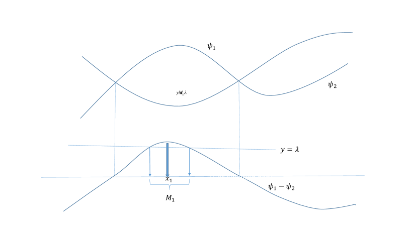
Figure 1: The optimal share $A_{1}$ of capacity $M_{1}$ is determined by the level line of $\psi_{1}-\psi_{2}\geq\lambda$, containing the maximal point $x_{1}$ of this function.

Example 2.2.

Suppose $\psi$ is a non-negative, continuous function on $X$ verifying $\mu(x;\psi(x)=r)=0$ for any $r\geq 0$. Let $\lambda_{N}>\lambda_{N-1}>\ldots\lambda_{1}>0$ be constants. We assume $\psi_{i}:=\lambda_{i}\psi$ verifies assumption 2.1.

From (3, 4) we obtain

$$A_{0}^{+}(\vec{p})\equiv\{x;\psi(x)<\min_{i\in I}\lambda_{i}^{-1}p_{i}\}\ ;\ \ A_{i}^{+}(\vec{p})\equiv\left\{x;\min_{j>i}\frac{p_{j}-p_{i}}{\lambda_{j}-\lambda_{i}}>\psi(x)>\max_{j<i}\frac{p_{j}-p_{i}}{\lambda_{j}-\lambda_{i}}\right\}-A_{0}^{+}(\vec{p})\ .$$

In particular, the partition $A_{i}^{+}(\vec{p})$ are consists of unions of level sets of the function $\psi$.

At optimal partition we observe that the share of the ”top agent” $N$ is just the level set

$$A_{N}:=A^{\bar{\lambda}_{N}}\equiv\left\{x\in X;\ \ \psi(x)\geq\bar{\lambda}_{N}\right\}\$$

where

$$\bar{\lambda}_{N}:=\sup\{\lambda;\mu(A^{\lambda})>M_{N}\}=\inf\{\lambda;\mu(A^{\lambda})<M_{N}\}\$$

(compare with (11, 12)). By induction we can proceed to find

$$A_{j}:=A^{\bar{\lambda}_{j+1},\bar{\lambda}_{{j}}}\equiv\left\{x\in X;\ \ \bar{\lambda}_{j+1}\geq\psi(x)\geq\bar{\lambda}_{j}\right\}\ ,$$ (13)

where $\bar{\lambda}_{j+1}$ is known by the induction step and

$$\bar{\lambda}_{j}:=\inf\{\lambda\geq 0;\mu(A^{\bar{\lambda}_{j+1},\lambda})<M_{j}\}\ .$$

An equivalent representation of the optimal partition is obtained as follows: Let $A_{s}:=\{x\in X;\psi(x)\leq s\}$, $f(s):=\mu(A_{s})$, $F(t):=\int_{0}^{t}f(s)ds$, $F^{*}(m):=\sup_{t\in\mathbb{R}}[mt-F(t)]$. Note that $F$ is a convex function and $F^{*}$ is its Legendre transform, which is convex as well and is defined on the interval $[0,\mu(X)]$. Moreover, by duality

$$F^{*}(\mu(A_{s}))\equiv\int_{A_{s}}\psi d\mu.$$

Given $\vec{M}\in\mathbb{R}^{N}_{+}$, let ${\cal M}_{N+1}:=\mu(X)$, ${\cal M}_{j}:=[{\cal M}_{j+1}-M_{j}]_{+}$ for $j=N,N-1,\ldots 1$. Then $\bar{\lambda}_{i}=F^{*}({\cal M}_{i})$, so (13) is written as

$$A_{i}:=\{x\in X;F^{*}({\cal M}_{i})<\psi(x)\leq F^{*}({\cal M}_{i+1})\}\ \ \ \ ;\ \ N\geq i\geq 1\ .$$

Note that the optimal partition does not depend on $\vec{\lambda}:=(\lambda_{1},\ldots,\lambda_{N})$, as there is no relation between $\lambda_{i}$ and $\bar{\lambda}_{i}$. However, the total profit $\Sigma_{\vec{\psi}}(\vec{M})$ does, of course, depend on $\vec{\lambda}$:

$$\Sigma_{\vec{\psi}}(\vec{M})=\sum_{i=1}^{N}\lambda_{i}\int_{A_{i}}\psi d\mu\equiv\sum_{i=1}^{N}\lambda_{i}(F^{*}({\cal M}_{i+1})-F^{*}\left({\cal M}_{i})\right)\ .$$ (14)

C.f Fig. 2.

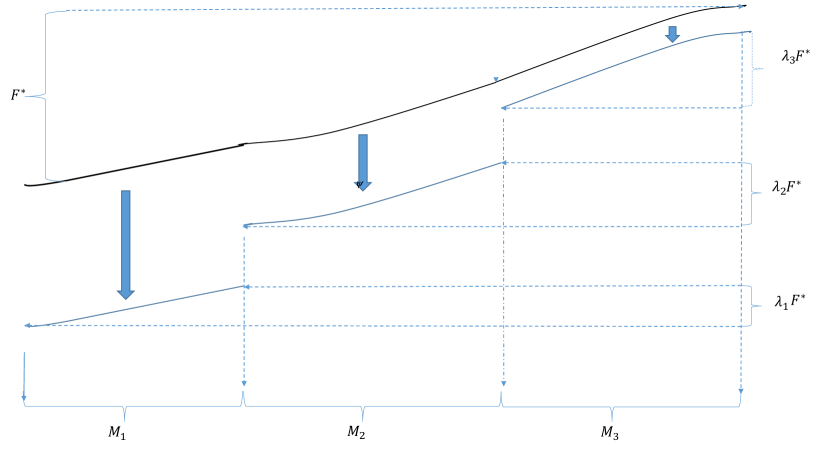
Figure 2: Representation of $s\mapsto F^{*}(s))$ corresponding to $\psi$, and optimal partition for $\psi_{i}=\lambda_{i}\psi$,$i=1,2,3$ subjected to capacities $\vec{M}=(M_{1},M_{2},M_{3})$ at saturation. Here $\lambda_{3}<1$.

3 Individual values

At the equilibrium price $\vec{p}_{0}$, the profit of agent $i$ is just $p_{0,i}\mu(A_{i}^{+}(\vec{p}_{0}))$. The profit gained by the set of her consumers $A_{i}^{+}(\vec{p}_{0})$ is

$$\int_{A^{+}_{i}(\vec{p}_{0})}\left(\psi_{i}(x)-p_{i,0}\right)d\mu\ .$$

The sum of the profits is

$$\bar{P}_{i}:=\int_{A_{i}^{+}(\vec{p}_{0})}\psi_{i}d\mu\ ,$$ (15)

which, by Theorem 1, equals the consumer’s part at the optimal partition $\bar{A}_{i}(\vec{M},\vec{\psi})$ in the ”Big Brother” paradigm given by (2). We denote $\bar{P}_{i}(\vec{M},\vec{\psi})$ as the individual value (i.v) of agent $i$, occasionally omitting its dependence on $\vec{M},\vec{\psi}$.

Assumption 3.1.

Let $(\vec{\psi},\vec{M})$ verify Assumption 2.1. Let $\tilde{\vec{\psi}}$ given by $\tilde{\psi_{i}}=\psi_{i}$ for $i\not=1$. In other words, the wisdom $\psi_{1}$ of agent 1 is replaced by $\tilde{\psi}_{1}$ while keeping $\psi_{i}$, $2\leq i\leq N$ and $\vec{M}$ unchanged. The new system $(\tilde{\vec{\psi}},\vec{M})$ verifies Assumption 2.1 as well. We denote $\tilde{P}_{1}$ the i.v of agent 1 after this change takes place.

Do wiser agents always get higher values?

Assuming a system of two agents in saturation and suppose that, after some education and training, agent $1$ improves her wisdom, so, in the notation of Assumption 3.1, $\tilde{\psi}_{1}\geq\psi_{1}$ on $X$. We expect that the i.v of the first agent $\bar{P}_{1}$ will increase under this change, so $\tilde{P}_{1}\geq\bar{P}_{1}$. Is it so, indeed?

Well, not necessarily! Suppose $M_{1}<<\mu(X)$ and let $x_{1}$ be a unique maximizer of $\psi_{1}-\psi_{2}$. According to Example 2.1, $\bar{P}_{1}\approx M_{1}\psi_{1}(x_{1})$. Let $\tilde{x}_{1}$ be a unique maximizer of $\tilde{\psi}_{1}-\psi_{2}$. Now, $\tilde{P}_{1}\approx M_{1}\tilde{\psi}_{1}(\tilde{x}_{1})$. But it may happen that $\tilde{\psi}_{1}(\tilde{x}_{1})<\psi_{1}(x_{1})$, even though $\tilde{\psi}_{1}>\psi_{1}$ everywhere!

Definitely, there are cases for which an increase in the wisdom of a given agent will increase her i.v, independently of her own capacity, as well as the wisdoms and capacity of the other agents. In particular, we can think about two cases where the above argument fails:

Case 1:  If $\tilde{\psi}_{1}=\psi_{1}+\lambda$, where $\lambda>0$ is a constant.

Case 2:  if $\tilde{\psi}_{1}=\beta\psi_{1}$, where $\beta\geq 2$ is a constant.

In the first case the ”gaps” $\psi_{1}-\psi_{2}$ and $\tilde{\psi}_{1}-\psi_{2}$ preserve their order, so if $x_{1}$ is a maximizer of the first, it is also a maximizer of the second. In particular the optimal partition $\bar{A}_{1},\bar{A}_{2}$ is unchanged, and we can even predict that $\tilde{P}_{1}=\bar{P}_{1}+\lambda M_{1}>\bar{P}_{1}$ (c.f Theorem 2 below).

In the second case the order of gaps may change. It is certainly possible that $\tilde{\psi}_{1}(\tilde{x}_{1})-\psi_{2}(\tilde{x}_{1})>\tilde{\psi}_{1}(x_{1})-\psi_{2}(x_{1})$ (where $x_{1}$, $\tilde{x}_{1}$ as above), but, if this is the case, an elementary calculation yields $\tilde{\psi}_{1}(\tilde{x}_{1})>\psi_{1}(x_{1})$, so the above argument fails. Indeed, if we assume both $\beta\psi_{1}(\tilde{x}_{1})-\psi_{2}(\tilde{x}_{1})>\beta\psi_{1}(x_{1})-\psi_{2}(x_{1})$ and $\beta\psi_{1}(\tilde{x}_{1})<\psi_{1}(x_{1})$, then $\psi_{1}(x_{1})-\psi_{2}(x_{1})<-\psi_{2}(\tilde{x}_{1})<\psi_{1}(\tilde{x}_{1})-\psi_{2}(\tilde{x}_{1})$ (since $\psi_{1}\geq 0$ and $\beta\geq 2$), so $x_{1}$ cannot be the maximizer of $\psi_{1}-\psi_{2}$ as assumed.

In fact, more can be said:

Theorem 2.

Under Assumption 3.1,

i) If $\tilde{\psi}_{1}=\beta\psi_{1}$ for a constant $\beta>0$ then $\tilde{P}_{1}\geq\beta\bar{P}_{1}$ if $\beta>1$, $\tilde{P}_{1}\leq\beta\bar{P}_{1}$ if $\beta<1$.

ii) In the saturation and under saturation cases, if $\tilde{\psi}_{1}=\psi_{1}+\lambda$ for a constant $\lambda>0$ then $\tilde{P}_{1}=\bar{P}_{1}+\lambda M_{1}$.

In Theorem 3 we expand on case (i) of Theorem 2 and obtain the following, somewhat surprising result:

Theorem 3.

Under Definition 3.1,

i) Suppose $\tilde{\psi}_{1}\geq\beta\psi_{1}$ where $\beta>1$ is a constant. Then

$$\tilde{P}_{1}\geq(\beta-1)\bar{P}_{1}\ .$$ (16)

ii) For any $\beta>2$, $s>\beta-1$ there exists such a system ($\vec{\psi},\vec{M}$) and $\tilde{\psi}_{1}\geq\beta\psi_{1}$ verifying Assumption 3.1 such that

$$\tilde{P}_{1}<s\bar{P}_{1}\ .$$

In particular, the inequality (16) is sharp in the case $\beta>2$.

Corollary 3.1.

The i.v of an agent cannot decrease if its wisdom $\psi_{i}$ is at least doubled ($\tilde{\psi}_{i}\geq 2\psi_{i}$).

In Theorem 4 we obtain sharp conditions for decrease of i.v, given an increase of the corresponding wisdom:

Theorem 4.

Under Assumption 3.1, in the under saturation/saturation cases:

i)If $1<\beta<2$, $\lambda\geq 0$ and

$$\beta\psi_{1}(x)\leq\tilde{\psi}_{1}(x)\leq\beta\psi_{1}(x)+\lambda\ ,$$ (17)

then

$$\tilde{P}_{1}\geq\bar{P}_{1}-\frac{M_{1}\lambda(2-\beta)}{\beta-1}\ .$$ (18)

ii) For any $1<\beta<2,\lambda>0,s<\lambda(2-\beta)/(\beta-1)$ there exists a system $(\vec{\psi},\vec{M})$ and
$\beta\psi_{1}\leq\tilde{\psi}_{1}\leq\beta\psi_{1}+\lambda$ verifying Assumption 3.1 such that

$$\tilde{P}_{1}<\bar{P}_{1}-M_{1}s\ \ .$$

In particular, the inequality (18) is sharp.

The proofs of Theorems 2-4 are given in Section 5.

4 Coalition/Partition games

4.1 Cartels and coalitions

Suppose that some agents $J\subset I$ decide to establish a cartel. In the free market interpretation it means that they coordinate the price of their services, i.e. $p_{i}:=p_{J}$ for some $p_{J}\in\mathbb{R}$ for any $i\in J$. In the big brother interpretation it means that $J$ is replaced by a single ”agent” whose capacity is

$$M_{J}:=\sum_{i\in J}M_{i}$$ (19)

and its wisdom is the maximal wisdom of its agents, namely

$$\psi_{J}(x):=\max_{i\in J}\psi_{i}(x)\ \ \ \forall x\in X\ \ .\$$ (20)

More generally, let ${\cal J}:=\{J_{1},\ldots J_{k}\}$ where $J_{i}\in 2^{I}$ a disjoint covering of $I$, that is

$$I=\cup_{i=1}^{k}J_{i}\ ,\ \ \ \ J_{i}\cap J_{l}=\emptyset\ \ \ \forall i\not=l\in\{1,\ldots k\}\$$

Let $M_{\cal J}:=\{M_{J_{1}},\ldots M_{J_{k}}\}$, $\psi_{\cal{J}}:=\{\psi_{J_{1}},\ldots\psi_{J_{k}}\}$. Let $\vec{1}^{(i)}\in\mathbb{R}^{N}$ given by $1^{(i)}_{j}=1$ if $j\in J_{i}$, $1^{(i)}_{j}=0$ if $j\not\in J_{i}$. Let $\mathbb{R}_{\cal{J}}:=\text{Span}\left\{\vec{1}^{(1)},\ \ldots\vec{1}^{(k)}\right\}\subset\mathbb{R}^{N}$. In analogy to (1) we set

$$\Sigma_{\psi_{\cal J}}(\vec{M}_{\cal J}):=\max_{\vec{A}\in{\cal P}_{\vec{M}_{\cal J}}}\sum_{J\in{\cal J}}P_{\psi_{J}}(A_{J})\ .\$$ (21)

$$\Xi^{0}_{\vec{\psi}_{\cal J}}(\vec{p}):=\int_{X}\max_{J\in{\cal J}}[\psi_{J}(x)-p_{J}]_{+}d\mu(x):\mathbb{R}^{k}\rightarrow\mathbb{R}\ .$$ (22)

Proposition 4.1.

Assume the conditions of Theorem 1. Given a partition $\cal{J}$ of $I$ as above, we get in the US,S cases

$$\Sigma_{\vec{\psi}_{\cal J}}(\vec{M}_{\cal J})=\min_{\vec{p}\in\mathbb{R}_{\cal{J}}}\Xi^{0}_{\vec{\psi}_{\cal J}}(\vec{p})+\vec{p}\cdot\vec{M}_{\cal J}\ .$$

where $\Xi^{0}_{\vec{\psi}_{J}}$ as defined in (22). In the OS case,

$$\Sigma_{\vec{\psi}_{\cal J}}(\vec{M}_{\cal J})=\max_{\vec{m}\leq\vec{M}}\min_{\vec{p}\in\mathbb{R}_{\cal{J}}}\Xi^{0}_{\vec{\psi}_{\cal J}}(\vec{p})+\vec{p}\cdot\vec{M}_{\cal J}\ .$$

In all cases there exists a unique equilibrium price vector $\vec{p}_{0}\in\mathbb{R}_{\cal J}$, and the corresponding partition is the unique partition verifying (21).

Proof.

First note that

$$\{x\in X;\psi_{J}(x)-\psi_{J^{{}^{\prime}}}(x)=r\}\subset\cup_{j\in J,i\in J^{{}^{\prime}}}\{x\in X;\psi_{j}(x)-\psi_{i}(x)=r\}$$

for any $J,J^{{}^{\prime}}\in\vec{J}$ so (6, 7) imply, for any $r\in\mathbb{R}$,

$$\mu(x;\psi_{J}(x)-\psi_{J^{{}^{\prime}}}(x)=r)=0\ \ ;\ \ \ \mu(x;\psi_{J}(x)=r)=0\ \ \forall\ J,\ J^{{}^{\prime}}\in{\cal J}\ .$$

Hence, the conditions of Theorem 1 hold for this modified setting. The only thing left to show is that for each $\vec{p}\in\mathbb{R}_{\cal{J}}$, the associated partition $\vec{A}^{+}(\vec{p})$ (c.f. 3, 4) is in ${\cal P}_{M_{\cal J}}$. This follows immediately from the following trivial identity: if $\vec{p}:=p_{J_{1}}\vec{1}^{(1)}+\ldots+p_{J_{k}}\vec{1}^{(k)}\in\mathbb{R}_{\cal{J}}$ then

$$\max_{j\in I}[\psi_{j}(x)-p_{j}]_{+}\equiv\max_{J\in{\cal J}}[\psi_{J}(x)-p_{J}]_{+}\ .$$

Thus, the Proposition follows from Theorem 1 applied to this modified system. ∎

Note that Proposition 4.1 does not say anything about the partition inside a coalition $J$. In fact, it determines only the set of consumers $\bar{A}^{+}_{J}$ of this coalition. In particular, the joint value of the coalition $J$ is

$$\bar{P}_{J}(\vec{M},\vec{\psi}):=\int_{\bar{A}^{+}_{J}}\psi_{J}d\mu\ .$$

Do the agents of this coalition benefit from their collaboration? A necessary condition for this is that the combined value of the coalition $J$ is, at least, not smaller than the sum of the values of its members standing alone, namely

$$\sum_{i\in J}\bar{P}_{\{i\}}(\vec{M},\vec{\psi})\leq\bar{P}_{J}(\vec{M},\vec{\psi})\ \ \ ?$$ (23)

where $\bar{P}_{\{i\}}(\vec{M},\vec{\psi})$ is the i.v of $i\in J$ determined by the assumption that the coalition $J$ is disintegrated and its members are competing as individuals. In order to test the inequality, suppose $N=3$ and $J_{1}=\{1,2\}$, $J_{2}=\{3\}$. Suppose further that $M_{2}$ is very small, so $\bar{P}_{2}(\vec{M},\vec{\psi})\approx 0$ while the i.v of agent 1, standing alone, is the same as her i.v if she competes with agent 3 only, and her wisdom is $\psi_{1}$.

On the other hand, the i.v. of the coalition $J$ is approximated by the i.v of agent 1 playing against agent 3, where now her wisdom is, by Proposition 4.1, $\psi_{1,2}:=\max(\psi_{1},\psi_{2})$. Hence (23) is reduced into

$$\bar{P}_{\{1\}}(M_{1},M_{3},\psi_{1},\psi_{3})\leq\bar{P}_{\{1\}}(M_{1},M_{3},\psi_{1,2},\psi_{3})\ \ ?$$ (24)

Since $\psi_{1,2}\geq\psi_{1}$ it raises the question of monotonicity of i.v with respect to their wisdom. We may question this intuition, based on Theorem 4 in Section 3.

4.2 Review on cooperative games

A cooperative game is a game where groups of players (”coalitions”) may enforce cooperative behavior, hence the game is a competition between coalitions of players, rather than between individual players.

This section is based on the monograph [12].

Definition 4.1.

A cooperative game (CG game) in $I:=\{1,\ldots N\}$ is given by a reward function $\nu$ on the subsets of $I$:

$$\nu:2^{I}\rightarrow\mathbb{R}\ \ ,\ \ \nu(\emptyset)=0\ .$$

Definition 4.2.

The core of a game $\nu:2^{I}\rightarrow\mathbb{R}_{+}$, $Core(\nu)$, is a set of vectors $\vec{x}:=(x_{1},\ldots x_{N})\in\mathbb{R}^{N}$ which satisfy the following conditions

$$\sum_{i\in I}x_{i}\leq\nu(I)$$ (25)

and

$$\forall J\subseteq I,\ \ \sum_{i\in J}x_{j}\geq\nu(J)\ .$$ (26)

The grand coalition $J=I$ is stable if the core is not empty.

Non-emptiness of the core guarantees that no sub-coalition $J$ of the grand coalition $I$ will be formed. Indeed, if such a sub-coalition $J$ is formed, its reward $\nu(J)$ is not larger than the sum of the rewards of its members, guaranteed by the grand coalition.

In many cases, however, the core is empty.

We can easily find a necessary condition for the core to be non-empty. Suppose we divide $I$ into a set of coalitions $J_{k}\subset I$ , $k=1,\ldots m$ such that $J_{k}\cap J_{k^{{}^{\prime}}}=\emptyset$ for $k\not=k^{{}^{\prime}}$ and $\cup_{k=1}^{m}J_{j}=I$.

Proposition 4.2.

For any such division, the condition

$$\sum_{k=1}^{m}\nu(J_{k})\leq\nu(I)$$ (27)

is necessary for the grand coalition to be stable.

Proof.

Suppose $\vec{x}\in Core(\nu)$. Let $\tilde{\nu}(J):=\sum_{i\in J}x_{i}$. Then $\tilde{\nu}(J)\geq\nu(J)$ for any $J\subseteq I$. If (27) is violated for some division $\{J_{1},\ldots J_{m}\}$, then $\sum_{k=1}^{m}\tilde{\nu}(J_{k})\geq\sum_{k=1}^{m}\nu(J_{k})>\nu(I)$. On the other hand, $\sum_{k=1}^{m}\tilde{\nu}(J_{k})=\sum_{i\in I}x_{i}\leq\nu(I)$, so we get a contradiction. ∎

Note that super-additivity

$$\nu(J_{1})+\nu(J_{2})\leq\nu(J_{1}\cup J_{2})\ \ \ \forall\ J_{1}\cap J_{2}=\emptyset$$ (28)

is a sufficient condition for (27). However, (28) by itself is not a sufficient condition for the stability of the grand coalition.

Example 4.1.

In case $N=3$ the game $\nu(1)=\nu(2)=\nu(3)=0$, $\nu(12)=\nu(23)=\nu(13)=3/4$, $\nu(123)=1$ is super-additive but its core is empty.

We may extend condition (27) as follows: A weak division is a function $\lambda:2^{I}\rightarrow\mathbb{R}$ which satisfies the following:

i)  For any $J\subseteq I$, $\lambda(J)\geq 0$.

ii)  For any $i\in I$, $\sum_{J\subseteq I;i\in J}\lambda(J)=1$.

A collection of such sets $\{J\subset I;\lambda(J)>0\}$ verifying (i,ii) is called a balanced collection [12].

We can think about $\lambda(J)$ as the probability of the coalition $J$. Note that any division $\{J_{1},\ldots J_{m}\}$ is, in particular, a weak division where $\lambda(J)=1$ if $J\in\{J_{1},\ldots J_{m}\}$, and $\lambda(J)=0$ otherwise.

It is not difficult to extend the necessary condition (27) to weak subdivisions as follows:

Proposition 4.3.

For any weak subdivision $\lambda$, the condition

$$\sum_{J\in 2^{I}}\lambda(J)\nu(J)\leq\nu(I)\$$ (29)

is necessary for the grand coalition to be stable.

The proof of Proposition 4.3 is a slight modification of the proof of Proposition 4.2.

However, (29) is also a sufficient condition for the stability of the grand coalition $I$. This is the content of Bondareva-Shapley Theorem [11], [26], [27]:

Theorem 5.

The grand coalition is stable if and only if it satisfies (29) for any weak division $\lambda$.

The condition of Theorem 5 is easily verified for super-additive game in case $N=3$.

Corollary 4.1.

A super additive cooperative game of 3 agents ($N=3$) admits a non-empty core iff

$$\nu(12)+\nu(13)+\nu(23)<2\nu(123)\ .$$ (30)

Indeed, it can easily be shown that all weak subdivision for $N=3$ are spanned by

$$\lambda(J)=1/2\ \ \text{if}\ \ J=(12),(13),(23)\ \ \ ;\ \ \ \lambda(J)=0\ \ \text{otherwise}\ ,$$

and the trivial ones.

4.3 Back to coalition/partition game

We define a cooperative game for the $N$ agents which is based on the following:

• Let $\vec{\psi}$ be a wisdom vector verifying Assumption 2.1, and $\vec{M}$ a capacity vector in saturation (i.e $\sum_{i\in I}M_{i}=\mu(X)$).

• Let $J\subseteq I$ be a coalition, and $J^{-}:=I-J$ is the complementary coalition.

• Consider the two superagents $J,J^{-}$ subjected to the capacities $M_{J},M_{J^{-}}$ and wisdoms $\psi_{J},\psi_{J^{-}}$ as defined in (19, 20).

• By Theorem 1 and Proposition 4.1 there exists a unique maximizer $\bar{A}_{J},\bar{A}_{J^{-}}$ of

  $$(A_{J},A_{J^{-}})\in{\cal P}_{M_{J},M_{J^{-}}}\mapsto\int_{A_{J}}\psi_{J}d\mu+\int_{A_{J^{-}}}\psi_{J^{-}}d\mu\ .$$

• Let $\bar{P}_{J}:=\int_{\bar{A}_{J}}\psi_{J}d\mu$ be the i.v of the coalition $J$ under optimal partition.

  Definition 4.3.

  A coalition/partition (CP) game is given by a function on the subsets of $I$:

  $$\nu:2^{I}\rightarrow\mathbb{R}_{+}\ \ ;\ \ \ \nu(J):=\bar{P}_{J}\ .$$

  In particular, $\nu(I)=\int_{X}\psi_{I}d\mu$, and $\nu(\emptyset)=0$.

Note that the CP game satisfies the following condition: For each $J\subset I$,

$$\nu(J)+\nu(J^{-})\leq\nu(I)\ \ \forall\ \ J\subset I\ ,$$ (31)

which is a necessary condition for super-additivity (28).

However, a CP game is not super-additive in general. In fact, the inequality (24) may be violated, as we know from Theorem 4.

There is a special case, introduced in Example 2.2, Section 2, for which we can guarantee super-additivity for PC game:

Assumption 4.1.

There exists non-negative $\psi:X\in C(X)$ satisfying $\mu(x;\psi(x)=r)=0$ for any $r\in\mathbb{R}$. The wisdoms $\psi_{i}$ are given by $\psi_{i}=\lambda_{i}\psi$ where $\vec{\lambda}:=(\lambda_{1},\ldots\lambda_{N})\in\mathbb{R}^{N}_{+}$ such that $0<\lambda_{1}<\ldots<\lambda_{N}$. We further assume the saturation case $\sum_{i=1}^{N}M_{i}=\mu(X)$.

Proposition 4.4.

Under assumption 4.1, for any $\vec{M}\in\mathbb{R}^{N}_{+}$, the corresponding CP game is super-additive.

Proof.

From Example 2.2 (in particular from (14)) we obtain that the i.v. of agent $i$ under optimal partition is

$$\bar{P}_{i}\equiv\lambda_{i}\left(F^{*}({\cal M}_{i+1})-F^{*}({\cal M}_{i})\right)\ .$$ (32)

Note that $F^{*}$ is convex on $[0,1]$ by Example 2.2. In addition, $F^{*}(0)=0$.

It follows that for any $\alpha,\beta>0$ such that $\alpha+\beta\leq 1$:

$$F^{*}(\alpha+\beta)\geq F^{*}(\alpha)+F^{*}(\beta)\ .$$ (33)

Indeed, since $F^{*}$ is convex

$$F^{*}(\alpha+\beta)\geq F^{*}(\alpha)+\beta(F^{*})^{{}^{\prime}}(\alpha)\ .$$ (34)

By the same argument

$$0=F^{*}(0)\geq F^{*}(\beta)-\beta(F^{*})^{{}^{\prime}}(\beta)\ .$$ (35)

Assuming, with no loss of generality, that $\alpha\geq\beta$, we get (33) from the convexity of $F^{*}$ which implies $(F^{*})^{{}^{\prime}}(\alpha)\geq(F^{*})^{{}^{\prime}}(\beta)$, together with (34, 35).

By the definition of the CP game and (32) we obtain that

$$\nu(J)=\lambda_{N}(F^{*}(\mu(X))-F^{*}(\mu(X)-M_{J}))\ \ \text{if}\ \ \{N\}\in J\ \ \ ;\ \ \\ \nu(J)=\lambda_{J}(F^{*}(M_{J})-F^{*}(0))\equiv\lambda_{J}F^{*}(M_{J})\ \ \text{if}\ \{N\}\not\in J\ .$$ (36)

where $\lambda_{J}:=\max_{i\in J}\lambda_{i}$.

Let now $J_{1},J_{2}\subset I$ such that $J_{1}\cap J_{2}=\emptyset$ (in particular, $M_{J_{1}}+M_{J_{2}}\leq\mu(X)$ since $\vec{M}$ is a saturated vector).

Assume first $\{N\}\not\in J_{1}\cup J_{2}$. Then from (36, 33)

$$\nu(J_{1}\cup J_{2})=\max(\lambda_{J_{1}},\lambda_{J_{2}})F^{*}(M_{J_{1}\cup J_{2}})=\max(\lambda_{J_{1}},\lambda_{J_{2}})F^{*}(M_{J_{1}}+M_{J_{2}})\\ \geq\lambda_{J_{1}}F^{*}(M_{J_{1}})+\lambda_{J_{2}}F^{*}(M_{J_{2}})=\nu(J_{1})+\nu(J_{2})\ .$$ (37)

Next, if, say, $\{N\}\in J_{1}$ then

$$\nu(J_{1}\cup J_{2})=\lambda_{N}(F^{*}(\mu(X))-F^{*}(\mu(X)-M_{J_{1}}+M_{J_{2}}))\ \ ,\ \ \nu(J_{1})=\lambda_{N}(F^{*}(\mu(X))-F^{*}(\mu(X)-M_{J_{1}}))\ \ ,$$

$$\nu(J_{2})=\lambda_{J_{2}}F^{*}(M_{J_{2}})\ ,$$

so

$$\nu(J_{1}\cup J_{2})-\nu(J_{1})-\nu(J_{2})\geq\lambda_{N}\left[F^{*}(1-M_{J_{1}})-F^{*}(M_{J_{2}})-F^{*}(1-(M_{J_{1}}+M_{J_{2}})\right]\geq 0\ ,$$

again, by (33). ∎

Under the assumption of Proposition 4.4 we may guess, intuitively, that the grand coalition is stable if the gap between the wisdoms of the agents is sufficiently large (so the other agents are motivated to join the smartest one), and the capacity of the wisest agent ($N$) is sufficiently small (so (s)he is motivated to join the others as well). Below we prove this intuition in the case $N=3$:

Proposition 4.5.

Under the assumption of Proposition 4.4 and $N=3$,

$$\frac{\lambda_{3}}{\lambda_{2}}>\frac{F^{*}(M_{1}+M_{2})}{F^{*}(M_{2})+F^{*}(M_{1})}$$

is a necessary and sufficient for the stability of the grand coalition (i.e the non-emptiness of a core). Here $F^{*}$ is as defined in Example 2.2 (Section 2).

Proof.

From Corollary 4.1 and Proposition 4.4 we have only to prove (30). Now,

$$\nu(123)=\lambda_{3}F^{*}(\mu(X))\ \ ,\nu(13)=\lambda_{3}(F^{*}(\mu(X))-F^{*}(M_{2})),\ \ \nu(23)=\lambda_{3}(F^{*}(\mu(X))-F^{*}(M_{1}))$$

and

$$\nu(12)=\lambda_{2}F^{*}(M_{1}+M_{2})\ .$$

The result follows from substituting the above in (30).

∎

5 Free Market vs. Big Brother: Duality

Here we verify the dual nature of the free-market/big brother formulation and prove Theorem 1. This duality is also the main tool for proving Theorems 3, 4. The key Lemmas for all these results are the following:

Lemma 5.1.

Let

$$\Xi_{\vec{\psi}}(\vec{p}):=\int_{X}\max_{i\in I}[\psi_{i}(x)-p_{i}]d\mu(x)\ .$$ (38)

where $\vec{\psi}:=\{\psi_{1},\ldots\psi_{N}\}$ satisfies (6). Then $\Xi_{\vec{\psi}}$ is convex on $\mathbb{R}^{N}$. Moreover, it is differentiable at any point and

$$\frac{\partial\Xi_{\vec{\psi}}}{\partial p_{i}}(\vec{p})=-\mu(A_{i}(\vec{p}))\ .\ \$$ (39)

Here

$$A_{i}(\vec{p}):=\{x\in X;\ \psi_{i}(x)-p_{i}<\psi_{j}(x)-p_{j}\ \ \forall j\not=i\}\ .$$ (40)

Proof.

Note that $A_{i}(\vec{p})$ are mutually disjoint and, by (6), $\mu(\cup_{i\in I}A_{i}(\vec{p}))=\mu(X)$.
Consider $\xi:X\times\mathbb{R}^{N}\rightarrow\mathbb{R}$ give by $\xi(x,\vec{p})=\max_{i\in I}[\psi_{i}(x)-p_{i}]$. Then $\xi$ is convex on $\mathbb{R}^{N}$ for any $x\in X$. Moreover,

$$\frac{\partial\xi}{\partial p_{i}}=\left\{\begin{array}[]{cc}-1\ if&x\in A_{i}(\vec{p})\\ 0\ if&\exists j\not=i,\ x\in A_{j}(\vec{p})\end{array}\right.\$$

In particular, the $\vec{p}$ derivatives of $\xi$ exists $\mu$ a.e in $X$, $\nabla_{\vec{p}}\xi\in\mathbb{L}_{1}(X)$ for any $\vec{p}\in\mathbb{R}^{N}$ and are uniformly integrable. Since $\Xi_{\vec{\psi}}:=\int_{X}\xi d\mu$ by definition, it is still convex in $\mathbb{R}^{N}$, its derivatives exists everywhere and $\nabla_{\vec{p}}\Xi_{\vec{\psi}}=\int\nabla_{\vec{p}}\xi(x,\vec{p})d\mu(x)$.

∎

Lemma 5.2.

Let $a>0$ and $\vec{\psi}:=\vec{\psi}(x,t):X\times[0,a]\rightarrow\mathbb{R}^{N}_{+}$ for any $t\in[0,a]$. Assume further that each component $t\mapsto\psi_{i}(x,t)$ is convex and differentiable for any $x\in\mathbb{R}^{N}$ and

$$\partial_{t}\psi_{i}:=\dot{\psi_{i}}\in\mathbb{L}^{\infty}(X\times[0,a])$$

for any $i\in I$. Then the functions

$$(\vec{p},t)\mapsto\Xi(\vec{p},t):=\int_{X}\max_{i\in I}[\psi_{i}(x,t)-p_{i}]d\mu(x)$$

is convex on $\mathbb{R}^{N}\times[0,a]$, and, if its $t$ derivative $\dot{\Xi}:=\partial_{t}\Xi$ exists at $(\vec{p},t)$ then

$$\dot{\Xi}(p,t)=\sum_{i\in I}\int_{A_{i}(\vec{p},t)}\dot{\psi}_{i}(x,t)d\mu$$ (41)

Here

$$A_{i}(\vec{p},t):=\{x\in X;\ \psi_{i}(x,t)-p_{i}>\psi_{j}(x,t)-p_{j}\ \ \forall j\not=i\}\ .$$ (42)

Proof.

The proof is basically the same as the proof of Lemma 5.1. Here we define $\xi:X\times\mathbb{R}^{N}\times[0,a]\rightarrow\mathbb{R}$ give by $\xi(x,\vec{p},t)=\max_{i\in I}[\psi_{i}(x,t)-p_{i}]$, and $\Xi(\vec{p},t):=\int_{X}\xi(x,\vec{p},t)d\mu(x)$. Again, $\xi$ is convex on $\mathbb{R}^{N}\times[0,a]$ for any $x\in X$ so $\Xi$ is convex on $\mathbb{R}^{N}\times[0,a]$ as well, while

$$\dot{\xi}=\left\{\begin{array}[]{cc}\dot{\psi}_{i}(x,t)\ \ \ if&x\in A_{i}(\vec{p},t)\\ 0\ \ \ if&\exists j\not=i,\ x\in A_{j}(\vec{p},t)\end{array}\right.\ \ \$$

implies (41). ∎

5.1 Proof of Theorem 1

Note the difference between $\Xi_{\vec{\psi}}$ (38) and $\Xi_{\vec{\psi}}^{0}$ (8). Observe that

$$\Xi_{\vec{\psi}}(\vec{p}+\alpha\vec{1})=\Xi_{\vec{\psi}}(\vec{p})-\alpha\mu(X)\ \ \ ;\ \ \ \vec{1}:=(1,\ldots 1)\in\mathbb{R}^{N}\ .$$ (43)

In particular $\nabla\Xi_{\vec{\psi}}(\vec{p})=\nabla\Xi_{\vec{\psi}}(\vec{p}+\gamma\vec{1})$ and, in the saturated case $\vec{M}\cdot\vec{1}=\mu(X)$:

$$\Xi_{\vec{\psi}}(\vec{p})+\vec{M}\cdot\vec{p}=\Xi_{\vec{\psi}}(\vec{p}+\gamma\vec{1})+\vec{M}\cdot(\vec{p}+\gamma\vec{1})$$

for any $\gamma\in\mathbb{R}$.

Remark 5.1.

In the saturation case it follows that $\vec{p}\mapsto\Xi_{\vec{\psi}}(\vec{p})+\vec{p}\cdot\vec{M}$ is invariant under the shift. In addition we observe that, for $-\gamma$ large enough, such that $A_{0}^{+}(\vec{p}+\gamma\vec{1})=\emptyset$,

$$\Xi^{0}_{\vec{\psi}}(\vec{p}+\gamma\vec{1})=\Xi_{\vec{\psi}}(\vec{p}+\gamma\vec{1})$$

(recall Remark 2.3). So, in the saturation case, we may replace $\Xi^{0}_{\vec{\psi}}$ by $\Xi_{\vec{\psi}}$ and restrict the domain of $\Xi_{\vec{\psi}}$ to

$$\vec{p}\in\mathbb{R}^{N}\ \ ,\ \ \vec{p}\cdot\vec{1}=0\ .$$ (44)

Remark 5.2.

We may actually unify the under-saturated and saturated cases (US+S). Indeed, in the under-saturated case we add the ”null agent” whose wisdom $\psi_{0}=0$ and whose capacity is $M_{0}:=\mu(X)-\sum_{i\in I}M_{i}$. In that case we restrict our domain $(p_{0},p_{1},\ldots p_{N})\in\mathbb{R}^{N+1}$ to $p_{0}=0$, and we get by definition (8, 38)

$$\Xi_{\vec{0,\psi}}(0,p_{1},\ldots p_{N})=\Xi_{\vec{\psi}}^{0}(p_{1},\ldots p_{N})\$$

Hence the proof of the first part (saturated case), given below, includes also the proof of the under-saturated case. The over-saturated case will be treated later on.

Let $\vec{A}$ be any partition in

$${\cal P}_{\vec{M}}:=\{\vec{A};\ \mu(A_{i})=M_{i}\ \ \text{and}\ \ \mu(A_{i}\cap A_{j})=0\ \ \text{if}\ \ i\not=j\in I\ .\}$$

Then

$$\Sigma_{\vec{\psi}}(\vec{A}):=\sum_{i\in I}\int_{A_{i}}\psi_{i}d\mu=\sum_{i\in I}\int_{A_{i}}(\psi_{i}-p_{i})d\mu+\vec{M}\cdot\vec{p}\\ \leq\sum_{i\in I}\int_{A_{i}}\max_{i\in i}(\psi_{i}-p_{i})d\mu+\vec{M}\cdot\vec{p}=\int_{X}\max_{i\in i}(\psi_{i}-p_{i})d\mu+\vec{M}\cdot\vec{p}:=\Xi_{\vec{\psi}}(\vec{p})+\vec{M}\cdot\vec{p}\ .$$ (45)

In particular

$$\bar{\Sigma}_{\vec{\psi}}(\vec{M}):=\sup_{\vec{A}\in{\cal P}_{\vec{M}}}\Sigma_{\vec{\psi}}(\vec{A})\leq\inf_{\vec{p}\in\mathbb{R}^{N}}\Xi_{\vec{\psi}}(\vec{p})+\vec{M}\cdot\vec{p}\ .$$ (46)

Suppose we prove the existence of a minimizer $\vec{p}_{0}$ to the right side of (46). Then, by Lemma 5.1 (39) we get

$$\frac{\partial\Xi_{\vec{\psi}}}{\partial p_{i}}(\vec{p}_{0})=-M_{i}\ \ \ i\in I.$$

Moreover, $\vec{A}(\vec{p}_{0})\in{\cal P}_{\vec{M}}$ is an optimal partition so there is an equality in (46). Conversely, if $\vec{A}\in{\cal P}_{\vec{M}}$ is an optimal partition then there is an equality in (45) so

$$\psi_{i}(x)-p_{0,i}=\max_{j\in I}(\psi_{j}(x)-p_{0,j})$$

for $\mu$ a.e. $x\in A_{i}$. Hence $A_{i}\subseteq A_{i}(\vec{p}_{0})$ (up to a negligible $\mu$ set). By (5) we know that $\mu(\cup_{i\in I}A_{i})=\mu(X)$ so $A_{i}=A_{i}(\vec{p}_{0})$, again up to a negligible $\mu$ set. In particular it follows that an optimal partition $\vec{\bar{A}}\in{\cal P}_{\vec{M}}$ for $\Sigma_{\vec{\psi}}$ is unique

We now prove the existence of such a minimizer $\vec{p}_{0}$. Let $\vec{p}_{n}$ be a minimizing sequence of $\vec{p}\mapsto\Xi_{\vec{\psi}}(\vec{p})-\vec{p}\cdot\vec{M}$, that is

$$\lim_{n\rightarrow\infty}\Xi_{\vec{\psi}}(\vec{p}_{n})+\vec{p}_{n}\cdot\vec{M}=\inf_{\vec{p}\in\mathbb{R}^{N}}\Xi_{\vec{\psi}}(\vec{p}_{n})+\vec{p}_{n}\cdot\vec{M}\ .$$

Let $\|\vec{p}\|_{2}:=(\sum_{i\in I}p^{2}_{i})^{1/2}$ be the Euclidian norm of $\vec{p}$. If we prove that for any minimizing sequence $\vec{p}_{n}$ the norms $\|\vec{p}_{n}\|_{2}$ are uniformly bounded, then there exists a converging subsequence whose limit is the minimizer $\vec{p}_{0}$, and we are done. This follows, in particular, since $\Xi_{\vec{\psi}}$ is a closed (lower-semi-continuous) function.

Assume there exists a subsequence along which $\|\vec{p}_{n}\|_{2}\rightarrow\infty$. Let $\hat{\vec{p}}_{n}:=\vec{p}_{n}/\|\vec{p}_{n}\|_{2}$. Then

$$\Xi_{\vec{\psi}}(\vec{p}_{n})+\vec{p}_{n}\cdot\vec{M}:=\left[\Xi_{\vec{\psi}}(\vec{p}_{n})-\vec{p}_{n}\cdot\nabla_{\vec{p}}\Xi_{\vec{\psi}}(\vec{p}_{n})\right]+\vec{p}_{n}\cdot\left(\nabla_{\vec{p}}\Xi_{\vec{\psi}}(\vec{p}_{n})+\vec{M}\right)\\ =\left[\Xi_{\vec{\psi}}(\vec{p}_{n})-\vec{p}_{n}\cdot\nabla_{\vec{p}}\Xi_{\vec{\psi}}(\vec{p}_{n})\right]+\|\vec{p}_{n}\|_{2}\hat{\vec{p}}_{n}\cdot\left(\nabla_{\vec{p}}\Xi_{\vec{\psi}}(\vec{p}_{n})+\vec{M}\right)\ .$$ (47)

Note that

$$\Xi_{\vec{\psi}}(\vec{p})-\vec{p}\cdot\nabla\Xi_{\vec{\psi}}(\vec{p})=\sum_{i\in I}\int_{A_{i}(\vec{p})}\psi_{i}d\mu\ ,$$ (48)

so, in particular

$$0\leq\int_{X}\min_{i\in I}\psi_{i}d\mu\leq\left[\Xi_{\vec{\psi}}(\vec{p})-\vec{p}\cdot\nabla_{\vec{p}}\Xi_{\vec{\psi}}(\vec{p})\right]=\sum_{i\in I}\int_{A_{i}(\vec{p})}\psi_{i}(x)d\mu\\ \leq\int_{X}\max_{i\in I}\psi_{i}d\mu<\infty\ .$$ (49)

By (47- 49) we obtain, for $\|\vec{p}_{n}\|_{2}\rightarrow\infty$,

$$\lim_{n\rightarrow\infty}\hat{\vec{p}}_{n}\cdot\left(\nabla_{\vec{p}}\Xi_{\vec{\psi}}(\vec{p}_{n})+\vec{M}\right)=0\ .$$ (50)

Since $\hat{\vec{p}}_{n}$ lives in the unit sphere $S^{N-1}$ (which is a compact set), there exists a subsequence for which $\hat{\vec{p}}_{n}\rightarrow\hat{\vec{p}}_{0}:=(\hat{p}_{0,1},\ldots\hat{p}_{0,N})\in S^{N-1}$. Let $P_{-}:=\min_{i\in I}\hat{p}_{i,0}$ and $J_{-}:=\{i\in I\ ;\hat{p}_{0,i}=P_{-}\}$.

Note that for $n\rightarrow\infty$ along such a subsequence, $p_{n,i}-p_{n,i\prime}\rightarrow\infty$ for $i\not\in J_{-},i\prime\in J_{-}$. It follows that $A_{i}(\vec{p}_{n})=\emptyset$ if $i\not\in J_{-}$ for $n$ large enough, hence $\mu(\cup_{i\in J_{-}}A_{i}(\vec{p}_{n}))=\mu(X)=\mu(X)$ for $n$ large enough. Let $\mu_{i}^{n}$ be the restriction of $\mu$ to $A_{i}(\vec{p}_{n})$. Then the limit $\mu^{n}_{i}\rightharpoonup\mu_{i}$ exists (along a subsequence) where $n\rightarrow\infty$. In particular, by Lemma 5.1

$$\lim_{n\rightarrow\infty}\frac{\partial\Xi_{\vec{\psi}}}{\partial p_{n,i}}(\vec{p}_{n})=-\lim_{n\rightarrow\infty}\int_{X}d\mu_{i}^{n}=-\int_{X}d\mu_{i}$$

while $\mu_{i}\not=0$ only if $i\in J_{-}$, and $\sum_{i\in J_{-}}\mu_{i}=\mu$. Since $\hat{\vec{p}}_{0,i}=P_{-}$ for $i\in J_{-}$ is the minimal value of the coordinates of $\hat{\vec{p}}_{0}$, it follows that

$$\lim_{n\rightarrow\infty}\hat{\vec{p}}_{n}\cdot\left(\nabla_{\vec{p}}\Xi_{\vec{\psi}}(\vec{p}_{n})+\vec{M}\right)=-\vec{M}\cdot\hat{\vec{p}}_{0}+P_{-}\sum_{i\in J_{-}}\int_{X}d\mu_{i}=-\vec{M}\cdot\hat{\vec{p}}_{0}+P_{-}\ .$$

Now, by definition, $\vec{M}\cdot\hat{\vec{p}}_{0}>P_{-}$ unless $J_{-}=I$. In the last case we obtain a contradiction of (44) since it implies $\hat{\vec{p}}_{0}=0$ which contradicts $\hat{\vec{p}}_{0}\in S^{N-1}$. So, if $J_{-}$ is a proper subset of $I$ we obtain a contradiction to (50). Hence $\|\vec{p}_{n}\|_{2}$ is bounded, and a minimizer $\vec{p}_{0}$ exists. This concludes the proof of the Theorem for the saturation and under saturation case (c.f. Remark 5.2).

To complete the proof for the over-saturation case we will show that the minimizer of (10) is unique. This follows from the strict concavity of the function $\vec{m}\mapsto\Sigma_{\vec{\psi}}(\vec{m})$ on the simplex

$$S_{N}:=\{\vec{m}\in\mathbb{R}^{N}_{+};\vec{m}\cdot\vec{1}\leq\mu(X)\}\ .$$ (51)

The proof of this strict concavity is given at the Appendix (Section 7). $\Box$

5.2 Individual values: Proof of Theorems 2, 3, 4

For these we will use Lemma 5.2 in addition to Lemma 5.1.

The proof of Theorem 2 is the easiest:

Proof.

of Theorem 2

i) Let $\vec{t}:=(t_{1},\ldots t_{N})\in\mathbb{R}^{N}$. Let $\vec{t}\otimes\vec{\psi}(x):=(t_{1}\psi_{1}(x),\ldots t_{N}\psi_{N}(x))$. Consider

$$\Xi(\vec{t},\vec{p}):=\Xi_{\vec{t}\otimes\vec{\psi}}(\vec{p})\ .$$ (52)

By Lemma 5.2, $(\vec{t},\vec{p})\mapsto\Xi$ is convex on $\mathbb{R}^{N}\times\mathbb{R}^{N}$ (in particular, convex in $\vec{p}$ for fixed $\vec{t}$ and convex in $\vec{t}$ for fixed $\vec{p}$). In addition

$$\partial_{t_{i}}{\Xi}(\vec{t},\vec{p})=\int_{A_{i}(\vec{p},\vec{t})}\psi_{i}d\mu\equiv t_{i}^{-1}P_{i}(\vec{t})$$ (53)

where

$$A_{i}(\vec{p},\vec{t}):=\{x\in X;\ t_{i}\psi_{i}(x)-p_{i}<t_{j}\psi_{j}(x)-p_{j}\ \ \forall j\not=1\}\ ,$$ (54)

whenever $\partial_{t_{i}}{\Xi}$ exists. Let

$$\Sigma(\vec{t},\vec{M}):=\min_{\vec{p}\in\mathbb{R}^{N}}\Xi(\vec{p},\vec{t})+\vec{M}\cdot\vec{p}\ .$$ (55)

Recall that $\Sigma(\vec{t},\vec{M})=-\infty$ unless $\vec{M}$ is saturated. Still, it is real valued, convex as a function of $\vec{t}$ for any saturated $\vec{M}$. If $\vec{M}$ is over-saturated then

$$\Sigma(\vec{t},\vec{M}):=\max_{\vec{m}\leq\vec{M}}\min_{\vec{p}\in\mathbb{R}^{N}}\Xi(\vec{p},\vec{t})+\vec{m}\cdot\vec{p}$$

is convex in $\vec{t}$ as well.

Then

$$\partial_{t_{i}}{\Sigma}=\int_{A_{i}(\vec{p}_{0},\vec{t})}\psi_{i}d\mu\equiv t_{i}^{-1}P(\vec{t})$$

holds, where $\vec{p}_{0}:=\vec{p}_{0}(\vec{M},\vec{t})$ is the unique equilibrium price vector (perhaps up to an additive constant) guaranteed by Theorem 1 for the utility vector $\vec{t}\otimes\vec{\psi}$. Since the derivative of a convex function on the line is monotone non-decreasing we get for $\vec{t}_{(\beta)}:=(\beta,1;\ldots 1)$, $\beta>1$

$$P_{1}(\vec{t}_{(\beta)})/\beta\equiv\partial_{\beta}{\Sigma}(\vec{t}_{(\beta)},\vec{M})\geq\partial_{s}{\Sigma}(\vec{t}_{(s=1)},\vec{M})\equiv\bar{P}_{1}$$

where $\tilde{P}_{1}\equiv P_{1}(\vec{t}_{(\beta)})$ by (53, 54). This completes the proof for saturated and over-saturated $\vec{M}$. The case of under-saturated $\vec{M}$ is included in the saturated case (c.f Remark 5.2).

ii) If $\psi_{1}\rightarrow\psi_{1}+\lambda$ then the optimal partition in the saturated and under saturated cases is unchanged. Then

$$\tilde{P}_{1}:=\int_{\bar{A}_{1}}(\psi_{1}+\lambda)d\mu=\int_{\bar{A}_{1}}\psi_{1}d\mu+\lambda\int_{\bar{A}_{1}}d\mu=\bar{P}_{1}+\lambda M_{1}\ .$$

∎

Proof.

of Theorem 3

i) Let $\sigma:=\tilde{\psi}_{1}-\beta\psi_{1}\geq 0$, $\alpha:=\beta-1\geq 0$ and a function $\phi:[0,1]\mapsto\mathbb{R}$ satisfying

$$\phi(0)=\dot{\phi}(0)=0\ \text{and}\ \ddot{\phi}\geq 0\ \ \text{for any}\ t\in[0,1]\ \ ,\ \phi(1)=1\ .$$ (56)

Define

$$\psi(x,t):=(1+\alpha t)\psi_{1}(x)+\sigma(x)\phi(t)\ .$$ (57)

So

$$\psi(x,1)=\tilde{\psi}_{1}(x)\$$ (58)

and $\psi$ is convex in $t\in[0,1]$ for any $x$. Also $\dot{\psi}(x,t)=\alpha\psi_{1}(x)+\sigma(x)\dot{\phi}(t)$. Let now $\delta>0$. Then

$$\psi(x,1)\geq\dot{\psi}(x,1)-\delta\|\sigma\|_{\infty}$$ (59)

provided

$$\sigma(x)\dot{\phi}(1)\leq\sigma(x)+\psi_{1}(x)+\delta\|\sigma\|_{\infty}\ .$$ (60)

Since $\psi_{1}$ and $\sigma$ are non-negative, the later is guaranteed if $\dot{\phi}(1)\leq 1+\delta$. So, we choose $\phi(t):=t^{1+\epsilon}$ for some $\epsilon\in(0,\delta]$. This meets (56,60).

Let now $\Sigma(\vec{M},t):=\Sigma_{\psi(,t),\psi_{2},\ldots\psi_{N}}(\vec{M})$. By Theorem 1,

$$\Sigma(\vec{M},t):=\inf_{\vec{p}\in\mathbb{R}^{N}}\Xi_{\vec{\psi}(\cdot,t)}(\vec{p})+\vec{p}\cdot\vec{M}$$

in the US, S cases and by Lemma 5.2, $(\vec{p},t)\mapsto\Xi_{\vec{\psi}(\cdot,t)}(\vec{p})$ is convex. So $\Sigma$ is convex in $t$. In the OS case

$$\Sigma(\vec{M},t):=\sup_{\vec{m}\leq\vec{M}}\inf_{\vec{p}\in\mathbb{R}^{N}}\Xi_{\vec{\psi}(\cdot,t)}(\vec{p})+\vec{p}\cdot\vec{m}$$

is convex (as maximum of convex functions) as well. By the same Lemma

$$\dot{\Sigma}(\vec{M},0)=\int_{\bar{A}_{1}(0)}\dot{\psi}(,0)d\mu=\alpha\int_{\bar{A}_{1}(0)}\psi_{1}d\mu\equiv\alpha\bar{P}_{1}$$ (61)

where $\bar{A}_{1}(0)$ is the first component in the optimal partition associated with $\vec{\psi}$, while, at $t=1$ we obtain from convexity and (59)

$$\dot{\Sigma}(\vec{M},1)=\int_{\bar{A}_{1}(1)}\dot{\psi}(x,1)d\mu\leq\int_{\bar{A}_{1}(1)}(\psi(x,1)+\delta\|\sigma\|_{\infty})d\mu\leq\int_{\bar{A}_{1}(1)}\psi(x,1)d\mu+\delta\|\sigma\|_{\infty}\$$ (62)

where $\bar{A}_{1}(1)$ is the first component in the optimal partition associated with
$\vec{\psi}(1):=(\psi(,1),\psi_{2},\ldots\psi_{N})$. Since $\tau\mapsto\phi(\tau)$ is convex, $\tau\mapsto\Sigma(\vec{M},\tau)$ is convex as well by Lemma 5.2 and we get

$$\dot{\Sigma}(\vec{M},1)\geq\dot{\Sigma}(\vec{M},0)\ .$$ (63)

From (62, 63)

$$\int_{\bar{A}_{1}(1)}\psi(x,1)d\mu\geq\alpha\bar{P}_{1}-\delta\|\sigma\|_{\infty}\ .$$

Now, recall $\beta:=1+\alpha$ and $\psi(x,1):=\tilde{\psi}_{1}$ by (58), so $\int_{\bar{A}_{1}(1)}\psi(x,1)d\mu\equiv\tilde{P}_{1}$. Since $\delta>0$ is arbitrary small, we obtain the result.

ii) Assume $N=2$, $M_{1}+M_{2}=\mu(X)$. We show the existence of non-negative, continuous $\psi_{1},\psi_{2}$, $x_{1},x_{2}\in X$ and $\lambda>0$ such that, for given $\delta>0$

a) $\Delta(x):=\psi_{1}(x)-\psi_{2}(x)<\Delta(x_{1})$ for any $x\in X-\{x_{1}\}$.

b) $\Delta_{\beta}(x):=\beta\psi_{1}(x)-\psi_{2}(x)<\Delta_{\beta}(x_{1})$ for any $x\in X-\{x_{1}\}$.

c) $\Delta_{\beta}(x_{2})+\lambda=\Delta_{\beta}(x_{1})+\delta$.

We show that (a-c) is consistent with

$$s\psi_{1}(x_{1})>\beta\psi_{1}(x_{2})+\lambda$$ (64)

for given $s>\beta-1$.

Suppose (64) is verified. Let

$$\theta_{0}:=\left\{\begin{array}[]{cc}1-\frac{|x-x_{2}|}{\epsilon}&\text{if}\ |x-x_{2}|\leq\epsilon\\ 0&\text{if}\ |x-x_{2}|>\epsilon\end{array}\right.$$ (65)

(assuming, for simplicity, that $X$ is a real interval). Set $\tilde{\psi}_{1}:=\beta\psi_{1}+\lambda\theta_{0}$. If $\epsilon$ is small enough then $\tilde{\psi}_{1}-\psi_{2}$ is maximized at $x_{2}$ by (b,c), while $\psi_{1}-\psi_{2}$ is maximized at $x_{1}$ by (a). Letting $M_{1}<<1$ we find, by Example 2.1, that $\bar{P}_{1}\approx M_{1}\psi_{1}(x_{1})$ and $\tilde{P_{1}}\approx M_{1}(\beta\psi_{1}(x_{2})+\lambda\theta_{0}(x_{2}))=M_{1}(\beta\psi_{1}(x_{2})+\lambda)$. By (64) we obtain the result.

So, we have only to prove that (64) is consistent with (a-c). We rewrite it as

$$\frac{s}{\beta-1}\left[\Delta_{\beta}(x_{1})-\Delta(x_{1})\right]>\frac{\beta}{\beta-1}\left[\Delta_{\beta}(x_{2})-\Delta(x_{2})\right]+\lambda\ .$$

From (c) we obtain

$$\frac{s}{\beta-1}\left[\Delta_{\beta}(x_{1})-\Delta(x_{1})\right]>\frac{\beta}{\beta-1}\left[\Delta_{\beta}(x_{2})-\Delta(x_{2})\right]+\Delta_{\beta}(x_{1})-\Delta_{\beta}(x_{2})+\delta\ ,$$

that is

$$(s-\beta+1)\Delta_{\beta}(x_{1})-\Delta_{\beta}(x_{2})>(s-\beta)\Delta(x_{2})+s(\Delta(x_{1})-\Delta(x_{2}))+\delta(\beta-1)\ .$$ (66)

We now set $\Delta_{\beta}(x_{1})$ and $\lambda$ large enough, keeping $\delta,\Delta_{\beta}(x_{2}),\Delta(x_{1}),\Delta(x_{2})$ fixed. Evidently, we can do it such that (c) is preserved. Since $s-\beta+1>0$ by assumption, we can get (66).

∎

Proof.

of Theorem 4.

i) Let $\beta=1+t$ where $t\in(0,1)$. We change (57) into

$$\psi(x,t):=(1+t)(\psi_{1}(x)+\gamma)+\sigma(x)\phi(t)$$ (67)

and

$$\tilde{\psi}_{1}:=(1+t)\psi_{1}+\sigma\phi(t)\$$ (68)

where $\gamma>0$ is a constant and $\sigma\geq 0$ on $X$. Then $\dot{\psi}(x,t)=\psi_{1}(x)+\gamma+\sigma(x)\dot{\phi}(t)$, and we obtain

$$\psi(x,t)\geq\dot{\psi}(x,t),\ \ t>0;\ \ \dot{\psi}(x,0)=\psi_{1}(x)+\gamma$$ (69)

provided

$$\sigma(x)\dot{\phi}(t)\leq\sigma(x)\phi(t)+t(\psi_{1}(x)+\gamma)\ ;\ \dot{\phi}(0)=0\ .$$ (70)

Since $\psi_{1},\sigma$ are non-negative, the later is guaranteed if

$$\dot{\phi}(t)\leq\phi(t)+\frac{t\gamma}{\|\sigma\|_{\infty}}\ ;\ \dot{\phi}(0)=0\ .$$ (71)

Since $t<1$, the choice $\phi(\tau):=\tau^{1+\epsilon}$ for $0\leq\tau\leq t$ and $\epsilon>0$ small enough (depending on $t$) verifies (71) provided

$$\|\sigma\|_{\infty}<\gamma t/(1-t)\ .$$ (72)

Hence we can let $\sigma$ to be any function verifying (72). Then (67, 68) imply

$$(1+t)\psi_{1}(x)\leq\tilde{\psi}_{1}(x)\leq(1+t)\psi_{1}(x)+\frac{\gamma t^{2+\epsilon}}{1-t}\ .$$ (73)

Now, we note from the second part of (69) that

$$\dot{\Sigma}(\vec{M},0)=\int_{\bar{A}_{1}(0)}\dot{\psi}(,0)d\mu=\int_{\bar{A}_{1}(0)}(\psi_{1}+\gamma)d\mu\equiv\bar{P}_{1}+\gamma M_{1}\$$ (74)

since $A_{1}(0)$ is independent of $\gamma$ in the S, US cases. In addition, (67, 68,71) imply

$$\dot{\Sigma}(\vec{M},t)=\int_{\bar{A}_{1}(t)}\dot{\psi}(,t)d\mu\leq\int_{\bar{A}_{1}(t)}\psi(\cdot,t)d\mu=\int_{\bar{A}_{1}(t)}(\tilde{\psi}_{1}+(1+t)\gamma)d\mu\equiv\tilde{P}_{1}+(1+t)\gamma M_{1}\ ,$$

where $\bar{A}_{1}(t)$ is the first component in the optimal partition associated with
$\vec{\psi}(t):=(\psi(,t),\psi_{2},\ldots\psi_{N})$. Since $\tau\mapsto\phi(\tau)$ is convex, $\tau\mapsto\Sigma(\vec{M},\tau)$ is convex as well by Lemma 5.2 and we get, as in (63)

$$\dot{\Sigma}(\vec{M},t)\geq\dot{\Sigma}(\vec{M},0)\ .$$ (75)

where, again, we used that $\bar{A}_{1}(t)$ is independent of $\gamma$ and $t>0$. Recalling $\beta:=1+t$, let $\lambda:=\gamma(\beta-1)^{2}/(2-\beta)$ and $\epsilon$ small enough we get (17, 18), using (73,74, 75).

ii) Assume $N=2$, $M_{1}+M_{2}=1$, that $\psi_{1}-\psi_{2}$ attains its maximum at $x_{1}$, and $x_{2}\not=x_{1}$. Let $\tilde{\psi}_{1}:=\beta\psi_{1}+\lambda\theta_{0}$ where $\theta_{0}$ as defined in (65). We assume, as in part (ii) of the proof of Theorem 3, that $x_{1}$ is a maximizer of $\beta\psi_{1}-\psi_{2}$ as well.

Next, assume

$$\beta\psi_{1}(x_{1})-\psi_{2}(x_{1})<\lambda+\beta\psi_{1}(x_{2})-\psi_{2}(x_{2})\$$ (76)

which implies, in particular, that $x_{2}$ is the maximizer of $\tilde{\psi}_{1}-\psi_{2}$ (see part (ii) of the proof of Theorem 3). If, in addition,

$$\psi_{1}(x_{1})-\beta\psi_{1}(x_{2})-\lambda-s>0\ ,$$ (77)

then, from Example 2.1,

$$\bar{P}_{1}\approx\psi_{1}(x_{1})M_{1}>M_{1}(\tilde{\psi}_{1}(x_{2})+s)\approx\tilde{P}_{1}+sM_{1}$$ (78)

if $M_{1}$ is small, and the proof is obtained.

From (76) and since $x_{1}$ is a maximizer of $\psi_{1}-\psi_{2}$:

$$\lambda>(\beta-1)(\psi_{1}(x_{1})-\psi_{1}(x_{2}))$$

so (77) and (76) are compatible provided

$$\lambda>(\beta-1)^{2}\psi_{1}(x_{2})+(\beta-1)\left[\lambda+s\right]\ ,$$

namely

$$\lambda\frac{2-\beta}{\beta-1}>(\beta-1)\psi_{1}(x_{2})+s\ .$$ (79)

Thus, if we assume further that, say, $\psi_{1}(x_{2})=0$ (which is consistent with the assumption that $\psi_{1},\psi_{2}\geq 0$) then (79) is verified for $s<\lambda(2-\beta)/(\beta-1)$.

∎

6 Conclusions and further study

We proved the existence of a unique, optimal partitions of a given set of consumers served by a finite set of agents of limited capacities, under certain conditions on their utilities (which were interpreted as the agent’s ”wisdoms”). This result enabled us to define an individual value of an agent and ask questions about the dependence of this individual value on her wisdom, where the capacities of all agents and wisdoms of all other agents are fixed.

Our definition of individual value can be questioned. In fact, the profit of an agent is just the price she charge per consumer, times the number of her consumers. Since, in our model, the capacity of agent $i$ is given by $M_{i}$ in the saturation and under saturation case, one may suggest to define her ”individual value” by

$$V^{a}_{i}:=M_{i}p^{0}_{i}$$

where $p_{i}^{0}$ is the price of her service at equilibrium. Another possible definition is the combined profit of her consumers, which is

$$V^{c}_{i}:=\int_{\bar{A}_{i}}(\psi_{i}(x)-p^{0}_{i})d\mu$$

where $\bar{A}_{i}$ is the share of agent $i$ under optimal partition. The individual value as defined in this paper is just the sum

$$\bar{P}_{i}=V^{a}_{i}+V^{c}_{i}\ .$$

More general definition of individual values can be obtained by different combination of these two values, such as

$$\bar{P}^{\alpha,\beta}_{i}:=\alpha V^{a}_{i}+\beta V^{b}_{i}\ ,$$

for given $\alpha,\beta\geq 0$.

However, the method used in this paper cannot be applied directly to the case $\alpha\not=\beta$. The reason is that all our results are strongly based on the convexity of $\Xi:=\Xi(\vec{t},\vec{p}):=\Xi_{\vec{t}\otimes\vec{\psi}}$ as a function of all it variables (see (52)). In fact, Theorems 2-4 are all based on the identity $\bar{P}_{i}:=P_{i}(\vec{1},\vec{M})$ for the individual value, where

$$P_{i}(\vec{t},\vec{M})=\frac{\partial\Sigma(\vec{t},\vec{M})}{\partial t_{i}}\$$

and $\Sigma(\vec{t},\vec{M}):=\min_{\vec{p}\in\mathbb{R}^{N}}\Xi(\vec{t},\vec{p})+\vec{p}\cdot\vec{M}$.

In order to extend our results to other definitions of individual value, say $V^{a}_{i}$, we my use the duality $p_{i}^{0}=\partial\Sigma/\partial M_{i}$ at $\vec{t}=\vec{1}$. Thus $V^{a}_{i}:=V_{i}^{a}(\vec{1},\vec{M})$ where

$$V_{i}^{a}(\vec{t},\vec{M}):=M_{i}\partial_{M_{i}}\Sigma(\vec{t},\vec{M})\$$

and $V^{b}_{i}:=V_{i}^{b}(\vec{1},\vec{M})$ where

$$V_{i}^{b}(\vec{t},\vec{M})=P_{i}(\vec{t},\vec{M})-V^{a}_{i}(\vec{t},\vec{M})\equiv\left(\partial_{t_{i}}-M_{i}\partial_{M_{i}}\right)\Sigma\ .$$

The dependence of $V^{a}_{i},V^{b}_{i}$ on the wisdom $\psi_{i}$ for prescribed capacities $\vec{M}$ is related to the behaviour of the functions $t_{i}\mapsto V_{i}^{a},V_{i}^{b}$ at fixed $\vec{M}$.

The difficulty in analyzing the dependence of either $V^{a}_{i}$ or $V^{c}_{i}$ on $\psi_{i}$ is originated from the fact that we do not have any general estimate on the dependence of the partial $M_{i}$ derivative of $\Sigma$ as functions of $t_{i}$. All we know about $\Sigma$ is that it is convex in $\vec{t}$ and concave in $\vec{M}$. On the other hand, the dependence of the individual value $\bar{P}_{i}$, as defined in this paper, is known due to the convexity of $\Sigma$ in the variables $\vec{t}$. Anyway, the analysis of the dependence of $V^{a}_{i},V^{b}_{i}$ on $\psi_{i}$ is worth studying, perhaps by numerical methods.

Acknowledgment: I would like to thank H. Brezis and R. Holtzmann for his helpful suggestion which contributed to the improvement of the results.

7 Appendix

We prove that the function $\vec{m}\mapsto\Sigma_{\vec{\psi}}(\vec{m})$ as defined in (10) is strictly concave on the simplex (51). To prove this we recall some basic elements form convexity theory (see, e.g. [16], [4]):

i)  If $F$ is a convex function on $\mathbb{R}^{N}$ (say), then the sub gradient $\partial F$ at point $p\in\mathbb{R}^{N}$ is defined as follows: $\vec{q}\in\partial F(\vec{p})$ if and only if

$$F(\vec{p}\prime)-F(\vec{p})\geq\vec{q}\cdot(\vec{p}\prime-\vec{p})\ \ \ \forall\vec{p}\prime\in\mathbb{R}^{N}\ .$$

ii) The Legendre transform of $F$:

$$F^{*}(\vec{q}):=\sup_{\vec{p}\in\mathbb{R}^{N}}\vec{p}\cdot\vec{q}-F(\vec{p})\ ,$$

and $Dom(F^{*})\subset\mathbb{R}^{N}$ is the set on which $F^{*}<\infty$.

iii) The function $F^{*}$ is convex (and closed), but $Dom(F^{*})$ can be a proper subset of $\mathbb{R}^{N}$ (or even an empty set).

iv) The subgradient of a convex function is non-empty (and convex) at any point in the proper domain of this function (i.e. at any point in which the function takes a value in $\mathbb{R}$).

v)  Young’s inequality

$$F(\vec{p})+F^{*}(\vec{q})\geq\vec{p}\cdot\vec{q}$$

holds for any pair of points $(\vec{p},\vec{q})\in\mathbb{R}^{N}\times\mathbb{R}^{N}$. The equality holds iff $\vec{q}\in\partial F(\vec{p})$, iff $\vec{p}\in\partial F^{*}(\vec{q})$.

vi)  The Legendre transform is involuting, i.e $F^{**}=F$ if $F$ is convex and closed.

Returning to our case, let $F(\vec{p}):=\Xi^{0}_{\vec{\psi}}(\vec{p})$. It is a convex function on $\mathbb{R}^{N}$ by Lemma 5.1. Moreover, its partial derivatives exists at any point in $\mathbb{R}^{N}$, which implies that its sub-gradient is s singleton. Recalling (9) with $\Xi_{\vec{\psi}}$ we get that

$$F^{*}(\vec{m})\equiv-\Sigma_{\vec{\psi}}(-\vec{m})$$

takes finite values only on the simplex (51). So, we only have to prove the existence of a unique minimizer (10) on the set $S_{N}\cap\{\vec{m}\leq\vec{M}\}$, which is a convex set as well. We prove below that $F^{*}$ is strictly convex on the simples. This implies the strict concavity of $\Sigma_{\vec{\psi}}$ on the same simplex.

Assume $F^{*}$ is not strictly convex. It means there exists $\vec{m}_{1}\not=\vec{m}_{2}\in S_{N}$ for which

$$F^{*}(\frac{\vec{m}_{1}+\vec{m}_{2}}{2})=\frac{F^{*}(\vec{m}_{1})+F^{*}(\vec{m}_{2})}{2}\ .$$ (80)

Let $\vec{m}:=\vec{m}_{1}/2+\vec{m}_{2}/2$, and $\vec{p}\in\partial F^{*}(\vec{m})$. Then, by (iv, v)

$$0=F^{*}(\vec{m})+F^{**}(\vec{p})-\vec{p}\cdot\vec{m}=F^{*}(\vec{m})+F(\vec{p})-\vec{p}\cdot\vec{m}\ .$$ (81)

By (80, 81):

$$\frac{1}{2}\left(F^{*}(\vec{m}_{1})+F(\vec{p})-\vec{p}\cdot\vec{m}_{1}\right)+\frac{1}{2}\left(F^{*}(\vec{m}_{2})+F(\vec{p})-\vec{p}\cdot\vec{m}_{2}\right)=0$$

while (v) also guarantees

$$F^{*}(\vec{m}_{i})+F(\vec{p})-\vec{p}\cdot\vec{m}_{i}\geq 0\ \ \ ,\ \ i=1,2\ .$$

It follows

$$F^{*}(\vec{m}_{i})-F(\vec{p})+\vec{p}\cdot\vec{m}_{i}=0\ \ \ ,\ \ i=1,2\ ,$$

so, by (v) again, $\{\vec{m}_{1},\vec{m}_{2}\}\in\partial F(\vec{p})$, and we get a contradiction since $\partial F(\vec{p})$ is a singleton.

References

- [1] L. Ambrosio: Lecture notes on optimal transport problems Mathematical Aspects of Evolving Interfaces, Lecture Notes in Math., Funchal, 2000, vol. 1812, Springer-Verlag, Berlin (2003), pp. 1-52
- [2] L. Ambrosio, L, N. Gigli and G. Savaré: Gradient flows in metric spaces and the Wasserstein spaces of probability measures, Lectures in Mathematics, ETH Zurich, Birkhauser, (2005).
- [3] Y. Brenier:, Polar factorization and monotone rearrangement of vector valued functions, Arch. Rational Mech &Anal., 122, (1993), 323-351
- [4] H.H Bauschke and P.L Combettes:, Convex Analysis and Monotone Operator Theory in Hilbert Spaces, Springer, (2011)
- [5] L.A. Caffarelli: The Monge-Ampere equation and optimal transportation, an elementary review, Optimal transportation and applications. Springer Berlin Heidelberg, 2003, 1-10
- [6] C Léonard: From the Schrödinger problem to the Monge-Kantorovich problem Journal of Functional Analysis Volume 262, Issue 4, 15 February (2012), 1879-1920
- [7] T. Champion and D.P. Luigi: On the twist condition and c-monotone transport plans, Discrete Contin. Dyn. Syst, 34, 4, (2012) 1339-1353,
- [8] P.A Chiappori , R. J. McCann, L. P. Nesheim:, Hedonic price equilibria, stable matching, and optimal transport: equivalence, topology, and uniqueness, Economic Theory 42.2 (2010): 317-354
- [9] G. Carlier:, Duality and existence for a class of mass transportation problems and economic applications , Advances in Mathematical Economics Volume 5, (2003), 1-21
- [10] S. Adams et al: Large deviations and gradient flows, Philosophical Transactions of the Royal Society A: Mathematical, Physical and Engineering Sciences 371.2005 (2013)
- [11] O. Bondareva, Certain applications of the methods of linear programming to the theory of cooperative games, Problemy Kibernetiki, 10 119-139 (in Russian), 1963
- [12] R. P. Gilles, The Cooperative Game Theory of Networks and Hierarchies, Series C: Game Theory, Mathematical programming and Operation research, V. 44, Springer 2010
- [13] T. Glimm and V. Oliker:, Optical design of single reflector systems and the Monge-Kantorovich mass transfer problem, Journal of Mathematical Sciences 117.3 (2003): 4096-4108
- [14] G. Monge: Mémoire sur la théorie des déblais et des remblais, In Histoire de lÁcadémie Royale des Sciences de Paris, 666-704, 1781
- [15] D.W Pentico:, Assignment problems: a golden anniversary survey, European J. Oper. Res. 176 (2007), no. 2, 774-793
- [16] H. Attouch: Variational Convergence for Functions and Operators, Pitman publishing limited, 1984
- [17] G. Carlier, A. Lachapelle: A Planning Problem Combining Calculus of Variations and Optimal Transport, Appl. Math. Optim. 63, , 1-9, 79-104. 2011
- [18] L.C Evans and W. Gangbo:, Differential equations methods for the Monge-Kantorovich mass transfer problem, Mem. Amer. Math. Soc. 137 (1999), no. 653, viii+66 pp
- [19] L.C. Evans:, Partial differential equations and Monge-Kantorovich mass transfer, Current Developments in Mathematics, Cambridge, MA, 1997, International Press, Boston, MA (1999), 65-126
- [20] W. Gangbo:, The Monge mass transfer problem and its applications, Monge Ampère equation: applications to geometry and optimization, (Deerfield Beach, FL, 1997), 79-104, Contemp. Math., 226, Amer. Math. Soc., Providence, RI, 1999
- [21] X.N. Ma, N. Trudinger and X.J. Wang:, Regularity of potential functions of the optimal transportation problem, Arch. Rational Mech. Anal., 177, 151-183, 2005
- [22] R. McCann and N. Guillen:, Five lectures on optimal transportation: Geometry, regularity and applications, http://www.math.cmu.edu/cna/2010CNASummerSchoolFiles/lecturenotes/mccann10.pdf
- [23] J. Rubinstein and G. Wolansky:, Intensity control with a free-form lens, J. Opt. Soc. Amer. A 24 (2007), no. 2, 463-469
- [24] J. Rubinstein and G. Wolansky: A weighted least action principle for dispersive waves, Ann. Physics 316 (2005), no. 2, 271-284
- [25] Y. Rubner, C. Tomasi and L. Guibas:, The Earth Mover’s Distance as a Metric for Image Retrieval, International Journal of Computer Vision, 40, 2, 99-121 (2000)
- [26] L.S. Shapley, On balanced sets and cores, Naval Research Logistics Quarterly, 14, 453-460, 1967
- [27] L.S. Shapley, Shapley, L. S. Cores of convex games, International Journal of Game Theory, 1, 11-26 1971
- [28] G. Wolansky: On Semi-discrete Monge Kantorovich and Generalized Partitions, to appear in JOTA
- [29] S. T. Rachev:, The Monge-Kantorovich Mass Transference Problem and Its Stochastic Applications, Theory of Probability & Its Applications, 1985, Vol. 29, 647-676
- [30] S.T Rachev and L.R Rüschendorf: , Mass Transportation Problems, Vol 1, Springer, 1998
- [31] C. Villani:, Topics in Optimal Transportation, Grad. Stud. Math., vol. 58 (2003)
- [32] C. Villani:, Optimal Transport: Old and New, Grundlehren der mathematischen Wissenschaften, (2008)