Geometrical measures of Non-Gaussianity generated from
single-field inflationary models

Abstract

We calculate the third-order moments of scalar curvature perturbations in configuration space for different inflationary models. We develop a robust numerical technique to compute the bispectrum for different models that have some features in the inflationary potential. From the bispectrum we evaluate moments analytically in the slow-roll regime while we devise a numerical mechanism to calculated these moments for non-slow-roll single-field inflationary models with a standard kinetic term that are minimally coupled to gravity. With the help of these third-order moments one can directly predict many non-Gaussian and geometrical measures of cosmic microwave background distributions in the configuration space. Thus, we devise a framework to calculate different third-order moments and geometrical measures, e.g. Minkowski functionals or the skeleton statistic, generated by different single-field models of inflation.

I Introduction

Recent results from ground- and balloon-based experiments as well as from WMAP and the Planck satellite have described the temperature anisotropies in the cosmic microwave background(CMB) with high precisionboom ; maxi ; cbi ; acbar ; wmap1 ; planck1 . This primordial CMB is close to being Gaussian however there are some features and anomalies that are unexplained as shown in Ref. planck4 and references therein. The study of non-Gaussian contributions in the cosmological perturbations is an ideal tool to study the inflationary dynamics. Among the most direct data sets for studies of inflation and non-Gaussianity are the CMB mapsplanck1 ; planck4 ; planck2 ; planck3 .

Inflation is the initial accelerated expansion of the early Universe. Inflationary expansion by more than $65$ $e$-folds is needed to explain the observed homogeneity and isotropy of the Universe. It is widely accepted that inflation is driven by the potential energy of a scalar inflaton field slowly rolling down the potential. Inflation also successfully describes the creation of small inhomogeneities, needed to seed observed structure in the Universe, as having been generated by quantum fluctuations in the inflaton field. The quantum fluctuations also got stretched and became imprinted on CMB maps and other observables on cosmological scales. Thus, inflation is able to explain not only why the Universe is so homogeneous and isotropic but also the origin of the structures in the Universe Guth1 ; Guth2 ; Linde3 ; mukhanov2 ; Bardeen2 ; starobinsky83 ; mukhanov . Alternatives to inflation have been proposed but no other scenario is as simple and elegant as inflation produced by scalar field(s)Linde1 ; Linde2 ; Kofman02 .

In single-field inflationary models generated inhomogeneities are described via a single scalar perturbation field $\zeta(\mathbf{x})$. The statistical properties of $\zeta(\mathbf{x})$ are the main observable signatures to distinguish inflationary models. We know that if the perturbations are exactly Gaussian then all odd $n$-point correlations functions vanish while all even $n$-point functions are related to the two-point function. Thus, in the momentum space the Gaussian field $\zeta$ is completely described by the power spectrum $P_{\zeta}(k)$,

$$\left\langle{\zeta}_{\mathbb{k}}{\zeta}_{\mathbb{k}^{\prime}}\right\rangle=(2\pi)^{3}\delta^{3}(\mathbb{k}+\mathbb{k}^{\prime})\frac{2\pi^{2}}{k^{3}}P_{\zeta}(k).$$ (1)

Inflation generally predicts that the power spectrum is nearly flat $P_{\zeta}(k)\propto k^{n_{s}-1}\approx\text{const}$ mukhanov2 ; starobinsky83 ; Bardeen2 . The fact that the observed scalar spectral index $n_{s}=0.9603\pm 0.0073$ planck2 is close to but not exactly unity is also considered by many to support the existence of inflation in the early Universe. However, many different kinds of inflationary models can be made compatible with observations of the power spectrum. Thus the study of the non-Gaussian signatures is important to reduce the degeneracy in inflationary models. Such signatures are contained in nontrivial higher-order correlations starting with the cubic ones.

Similar to the power spectrum, for three-point correlations one can calculate the bispectrum $B_{\zeta}(k_{1},k_{2},k_{3})$ as a measure of the non-Gaussianity of the initial perturbations

$$\left\langle\zeta_{\mathbb{k}_{1}}\zeta_{\mathbb{k}_{2}}\zeta_{\mathbb{k}_{3}}\right\rangle=(2\pi)^{3}\delta^{3}(\mathbb{k}_{1}+\mathbb{k}_{2}+\mathbb{k}_{3})B_{\zeta}(k_{1},k_{2},k_{3})~{}.$$ (2)

The bispectrum carries much more information than the power spectrum as it contains three different length scales. It is thought that for basic single-field slow-roll inflation with a standard kinetic term the non-Gaussian effects are small maldacena , there are many models of inflation that give large, potentially detectable, non-Gaussianity. Comparing non-Gaussian predictions with observations will help us to constrain or rule out different inflationary models and give us more insight about the physics of the early Universe.

In this paper we will focus on the study of non-Gaussianity through geometrical measures that describe visual properties of the initial perturbations viewed as a random field. Examples of standard measures of random fields are Minkowski functionals, extrema statistics and also more novel measures such as skeleton statistics. The simplest Minkowski functional is the Euler characteristic or genus density of excursion sets as a function of threshold. It has been shown that for mildly non-Gaussian field such local geometrical characteristics can be expressed as a series of higher order moments to the perturbation field and its derivatives Matsubara1 ; Bardeen3 ; PGP09 ; PPG11 ; Pogosyan1 ; Pogosyan2 . In particular for the Euler characteristic Matsubara1 ; PGP09

$$\chi_{\textsc{3D}}(\nu)\approx\left(\frac{\sigma_{1}}{\sqrt{3}\sigma}\right)^{3}\frac{e^{-\frac{\nu^{2}}{2}}}{(2\pi)^{2}}\Bigg{[}H_{2}(\nu)+\sigma\left(\frac{\left\langle\zeta^{3}\right\rangle}{6\sigma^{4}}H_{5}(\nu)\right.\Bigg{.}$$

$$\Bigg{.}\left.-\frac{3\left\langle\zeta^{2}\Delta\zeta\right\rangle}{4\sigma^{2}\sigma_{1}^{2}}H_{3}(\nu)-\frac{9\left\langle(\nabla\zeta)^{2}\Delta\zeta\right\rangle}{4\sigma_{1}^{4}}H_{1}(\nu)\right)\Bigg{]}\quad$$ (3)

In the above expression $\sigma^{2}=\left\langle\zeta^{2}\right\rangle$, $\sigma_{1}^{2}=\left\langle(\nabla\zeta)^{2}\right\rangle$, $\nu$ is the threshold in units of $\sigma$ and $H_{i}(\nu)$ are Hermite polynomials. The first term in the expansion denotes the Gaussian part that is proportional to $H_{2}(\nu)$ while other terms represent the first non-Gaussian correction in $\sigma$.

In this paper we have develop a robust mechanism to compute the third-order moments such as $\left\langle\zeta^{3}\right\rangle$, $\left\langle\zeta^{2}\Delta\zeta\right\rangle$ and $\left\langle(\nabla\zeta)^{2}\Delta\zeta\right\rangle$ for single-field models of inflation. This links the non-Gaussianity generated by inflation to the geometrical observables such as Euler characteristics and Minkowski functionals.

This paper is organized into six sections. In Sec. II, we review the theoretical framework of inflationary cosmology whereafter we will describe the calculation of the three-point correlation function in momentum space and the calculation of different third-order moments in configuration space. In Sec. III, we will present our numerical technique for the calculation of three-point function and briefly discuss different single-field models of inflation with some features in the inflationary potential. In Sec. IV, we will present the calculation of moments in configuration space while in Sec. V we present the geometrical Minkowski functionals. In the last section we will summarize our results and conclude with plans for future work.

II Theoretical Framework

single-field inflation driven by a scalar field $\phi$ is described by the following action in units of ($M_{pl}^{-2}=8\pi G=1$, $c=\hbar=1$)

$$S=\int d^{4}x\sqrt{-g}\left(\frac{1}{2}R-\frac{1}{2}g^{\mu\nu}\partial_{\mu}\phi\partial_{\nu}\phi-V(\phi)\right)$$ (4)

where $V(\phi)$ is the potential for the inflaton field. In Friedmann cosmology with homogeneous and isotropic background, the Friedmann equation for scale factor and Kline-Gordon equation for inflaton field are given by

$$H^{2}=\frac{1}{3}\left(\frac{1}{2}\dot{\phi}^{2}+V(\phi)\right)$$

$$\ddot{\phi}+3H\dot{\phi}+V_{,\phi}=0~{}.$$ (5)

One can define the following slow roll parameters and the corresponding slow roll conditions as

$$\epsilon=-\frac{\dot{H}}{H}\ll 1\text{, }\eta=\frac{\dot{\epsilon}}{\epsilon H}\ll 1~{}.$$ (6)

These slow roll conditions $\epsilon\ll 1,\eta\ll 1$ ensure that the inflaton field rolls slowly down the potential and the Universe inflates for significantly long period. These slow roll parameters depend on potential of the inflaton field and the model of inflation. For standard single-field inflation with quadratic potential $V(\phi)=\frac{1}{2}m^{2}\phi^{2}$ these slow roll parameters are of order $O(0.01)$ for inflaton field values $\phi>10M_{p}$.

II.1 Calculation of 2-point and 3-point Functions in Momentum Space

In this sections we will present the steps laid down by Maldacena to calculate the two-point and the three-point correlation function of the scalar perturbations maldacena . Firstly, one writes the action for the inflaton field given in Eq. 4 using the Arnowitt-Deser-Misner(ADM) formalism. Secondly, one expands the action to second order in perturbation theory for calculation of two-point function and to third-order for the calculation of three-point function. Thirdly, one quantizes the perturbations and imposes canonical commutation relations. Next, one can define the vacuum state by matching the mode function to Minkowski vacuum when the mode is deep inside the horizon that fixes the mode function completely. Following these steps one can find the power spectrum and the Bi-spectrum for scalar perturbations maldacena ; baumann1 .

In the ADM formalism the space-time is sliced into three-dimensional hyper-surfaces $\Sigma$, with three metric $g_{ij}$, at constant time. The line element of the space-time is given by

$$ds^{2}=-N^{2}dt^{2}+g_{ij}(dx^{i}+N^{i}dt)(dx^{j}+N^{j}dt)$$ (7)

where $N$ and $N^{i}$ and lapse and shift functions. In single-field inflation, we only have one physically independent scalar perturbation. Thus, we perturb the metric and matter part of the action and use the gauge freedom to choose the comoving gauge for the dynamical fields $\phi$ and $g_{ij}$

$$\delta\phi=0, g_{ij}=a^{2}(e^{2\zeta}\delta_{ij}+t_{ij})~{},$$ (8)

where $\zeta$ is the comoving curvature perturbation at constant density hyper-surface $\delta\phi=0$. In this gauge, the inflaton field is unperturbed and all scalar degrees of freedom are parameterized by the metric fluctuations $\zeta(t,x)$ while the tensor perturbations are parameterized by $t_{ij}$, that is both traceless and orthogonal $\partial_{i}t_{ij}=t^{i}_{i}=0$. The conditions in Eq. 8 fixes the gauge completely at non zero momentum maldacena . The shift and lapse functions are not dynamical variables in ADM formalism hence they can be derived from constraint equations in terms of $\zeta$. We shall only study scalar perturbations in this paper.

Linear perturbation results are obtained if one expand the action to second order in perturbation field $\zeta$

$$S_{(2)}=\int d^{4}xa^{3}\epsilon\left(\dot{\zeta}^{2}-a^{-2}(\partial\zeta)^{2}\right)$$ (9)

which gives the following equation of motion for scalar perturbations $v=z\zeta$ is Fourier space

$$v^{\prime\prime}_{\mathbb{k}}+\left(k^{2}-\frac{z^{\prime\prime}}{z}\right)v_{\mathbb{k}}=0.$$ (10)

where $z=a\dot{\phi}/H$ and momentum $k$ is in reduced Planck units $M_{pl}$. This is known as the Mukhanov equation for scalar perturbationsmukhanov3 . Now, one can calculate the 2-point function and the power spectrum

$$\left\langle\hat{\zeta}_{\mathbb{k}}\hat{\zeta}_{\mathbb{k}^{\prime}}\right\rangle=(2\pi)^{3}\delta^{3}(\mathbb{k}-\mathbb{k}^{\prime})\frac{2\pi^{2}}{k^{3}}P_{\zeta}(k)$$

$$P_{\zeta}(k)=\frac{k^{3}}{2\pi^{2}}|u_{k}|^{2}$$ (11)

where $u_{k}=v_{k}/z$ are the Fourier coefficients of $\zeta(x)$, the curvature perturbations.

To obtain next order results in perturbation theory and to calculate non-Gaussianity, one expands the action to third-order in scalar perturbations in comoving gaugemaldacena ; DSeery . After several integrations by parts and dropping the total derivatives one finds the following third-order action is often quoted in the literaturemaldacena ; DSeery

$$S_{(3)} = \int d^{4}x\bigg{(}a^{3}\epsilon^{2}\zeta\dot{\zeta}^{2}+a\epsilon^{2}\zeta(\partial\zeta)^{2}-2a\epsilon\dot{\zeta}(\partial_{i}\zeta)(\partial_{i}\chi)\bigg{.}$$ (12)

$$+ \frac{a^{3}}{2}\epsilon\dot{\eta}\zeta^{2}\dot{\zeta}+\frac{1}{2a}\epsilon(\partial_{i}\zeta)(\partial_{i}\chi)\partial^{2}\chi+\frac{1}{4a}\epsilon(\partial^{2}\zeta)(\partial^{2}\chi)^{2}$$

$$+ \left.2f(\zeta)\frac{\delta L}{\delta\zeta}\right)\quad$$

where the last term is variation of quadratic action is given by

$$\frac{\delta L}{\delta\zeta} = a\left(\frac{d\partial^{2}\chi}{dt}+H\partial^{2}\chi-\epsilon\partial^{2}\zeta\right)\text{, }\partial^{2}\chi=\epsilon a^{2}\dot{\zeta}$$

$$f(\zeta) = \frac{\eta}{4}\zeta^{2}+\text{terms with derivatives of }\zeta.$$ (13)

Now, the calculation of the three-point function from the above action involves integration over the time variable. But, if we use the action in Eq. 12 to calculate the three-point function, the integral over time does not converge to the end of inflation as pointed out by Arroja . However, it was shown inArroja ; Horner1 ; DSeery2 that this action can be converted into an equivalent form, that gives a convergent three-point function, by adding a total derivative term that is given by

$$-\frac{d}{dt}\left(\frac{\eta}{2}\epsilon a^{3}\zeta^{2}\dot{\zeta}\right)$$ (14)

which brings the action to the following form.

$$S_{(3)} = \int d^{4}x\bigg{(}a^{3}\epsilon(\epsilon-\eta)\zeta\dot{\zeta}^{2}+a\epsilon^{2}\zeta(\partial\zeta)^{2}-\frac{a}{2}\epsilon\eta\zeta^{2}\partial^{2}\zeta-2a\epsilon\dot{\zeta}(\partial_{i}\zeta)(\partial_{i}\chi)+\frac{1}{2a}\epsilon\partial^{2}\chi(\partial_{i}\zeta)(\partial_{i}\chi)+\frac{1}{4a}\epsilon(\partial^{2}\zeta)(\partial_{i}\chi)^{2}\bigg{.}$$ (15)

. $$+ 2g(\zeta)\frac{\delta L}{\delta\zeta}\bigg{)},\quad g(\zeta)=\zeta\dot{\zeta}/H+\frac{1}{4a^{2}H^{2}}\left[-(\partial\zeta)^{2}+\partial^{-2}(\partial_{i}\partial_{j}(\partial_{i}\zeta\partial_{j}\zeta))\right]+\frac{1}{4a^{2}H}\left[-(\partial\zeta)(\partial\chi)+\partial^{-2}(\partial_{i}\partial_{j}(\partial_{i}\zeta\partial_{j}\chi))\right]$$

Here the last term can be eliminated with a field redefinition $\zeta\rightarrow\zeta_{n}+g(\zeta)$ because $g(\zeta)$ is only a function of derivatives of scalar perturbations $\zeta(t,x)$ that vanish outside the horizon. The above third-order action is an exact result without any slow roll approximations thus it is even valid for models that deviate from slow roll conditions. Another feature of this action is that it contains only first two slow roll parameters $\epsilon$ and $\eta$ while it is independent of derivative terms such as $\eta^{\prime}$.

Finally, to calculate the 3-point function in momentum space we move to the interaction picture and write the Hamiltonian for the action in Eq. 4 as

$$H(\zeta)=H_{0}(\zeta)+H_{int}(\zeta)$$ (16)

where $H_{0}$ is the quadratic part of the Hamiltonian while $H_{int}$ represents all higher order terms in perturbation theorymaldacena . The three-point function in the interaction vacuum at some time $\tau$ near the end of inflation is given by

$$\left\langle\zeta_{\mathbb{k}_{1}}(\tau)\zeta_{\mathbb{k}_{2}}(\tau)\zeta_{\mathbb{k}_{3}}(\tau)\right\rangle=$$

$$-i\int_{\tau_{o}}^{\tau}d\tau^{\prime}a\left\langle\left[\zeta_{\mathbb{k}_{1}}(\tau)\zeta_{\mathbb{k}_{2}}(\tau)\zeta_{\mathbb{k}_{3}}(\tau),H_{int}(\tau^{\prime})\right]\right\rangle$$ (17)

To calculate 3-point function, the interaction Hamiltonian $H_{int}$ is just equal to $-S_{(3)}$ without the integral over time coordinate since the conjugate momenta vanish in the ADM formalism. Next, we quantize the perturbation field $\zeta(x)$ and define the vacuum state. For this we expand the $\zeta(x)$ field into creation and annihilation operators and use commutation relations of scalar field $\left[\hat{a}_{k},\hat{a}_{k^{\prime}}^{\dagger}\right]=\delta_{kk^{\prime}}$ to get the following result

$$\left\langle\zeta_{\mathbb{k}_{1}}\zeta_{\mathbb{k}_{2}}\zeta_{\mathbb{k}_{3}}\right\rangle=i(2\pi)^{3}\int_{-\infty}^{\tau_{end}}d\tau\left(-2a^{2}\epsilon^{2}u^{*}_{1}u^{\prime*}_{2}u^{\prime*}_{3}\frac{\mathbb{k}_{1}.\mathbb{k}_{2}}{k_{2}^{2}}\right.$$

$$\left.+2a^{2}\epsilon(\epsilon-\eta)u^{*}_{1}u^{\prime*}_{2}u^{\prime*}_{3}-a^{2}\epsilon(2\epsilon\mathbb{k}_{1}.\mathbb{k}_{2}+\eta k_{3}^{2})u^{*}_{1}u^{*}_{2}u^{*}_{3}\right.$$

$$+\frac{a^{2}}{2}\epsilon^{3}u^{*}_{1}u^{\prime*}_{2}u^{\prime*}_{3}k_{1}^{2}\frac{\mathbb{k}_{2}.\mathbb{k}_{3}}{k_{2}^{2}k_{3}^{2}}+\frac{a^{2}}{2}\epsilon^{3}u^{*}_{1}u^{\prime*}_{2}u^{\prime*}_{3}\frac{\mathbb{k}_{1}.\mathbb{k}_{2}}{k_{2}^{2}}+c.c.$$

$$\bigg{.}+\text{distinct permutations}\bigg{)}\left.\prod_{i=1}^{3}u_{i}(\tau_{end})\right.\delta^{3}(\sum_{j}\mathbb{k}_{j})\quad$$ (18)

The choice of the vacuum is specified by the choice of mode function $u_{k}$ selection. This is the main formula for the three-point function. This expression will be used in the sections to come for the exact numerical calculation of three-point function in momentum space.

II.2 Non-Gaussian parameters and $f_{\textsc{NL}}$

The integral relation for 3-point function given in Eq. 18 can be analytically evaluated in the slow roll limit. Ignoring $\epsilon^{3}$ terms in Eq. 18, gives us the following result that was first derived by Maldacenamaldacena .

$$\left\langle\zeta_{\mathbb{k}_{1}}\zeta_{\mathbb{k}_{2}}\zeta_{\mathbb{k}_{3}}\right\rangle=(2\pi)^{7}\delta^{3}(\mathbb{k}_{1}+\mathbb{k}_{2}+\mathbb{k}_{3})\frac{(P_{k}^{\zeta})^{2}}{\prod_{i}k_{i}^{3}}\mathcal{A}$$ (19)

$$\mathcal{A}=\frac{\eta^{*}-\epsilon^{*}}{8}\sum_{i}k_{i}^{3}+\frac{\epsilon^{*}}{8}\sum_{i\neq j}k_{i}k_{j}^{2}+\frac{\epsilon^{*}}{K}\sum_{i>j}k_{i}^{2}k_{j}^{2}\quad$$ (20)

where $*$ denotes the $\epsilon$ and $\eta$ values at horizon crossing. The quantity $\mathcal{A}$ is a convenient measure of non-Gaussianity in the perturbation field. The relationship between $\mathcal{A}$ and bispectrum is given by

$$B_{\zeta}(k_{1},k_{2},k_{3})=(2\pi)^{4}\frac{(P_{k}^{\zeta})^{2}}{\prod_{i}k_{i}^{3}}\mathcal{A}.$$ (21)

The bispectrum and $\mathcal{A}$ are general measures of non-Gaussianity however both these quantities are highly scale dependent. Thus, the three-point correlation is often described in terms of a local dimensionless non-linearity parameter $f_{\textsc{NL}}$. This non-linearity parameter $f_{\textsc{NL}}$ was first introduced as a measure of local non-Gaussianity described by

$$\zeta(x)=\zeta_{L}(x)-\frac{3}{5}f_{\textsc{NL}}\left(\zeta_{L}(x)^{2}-\left\langle\zeta_{L}(x)^{2}\right\rangle\right)~{},$$ (22)

where factor $\frac{3}{5}$ is a matter of convention. For local non-Gaussianity, the quantity $\mathcal{A}$ is expressed via the non linearity parameter $f_{\textsc{NL}}$ as

$$\mathcal{A}_{local}=-\frac{3}{10}f_{\textsc{NL}}\sum_{i}k_{i}^{3}~{}.$$ (23)

Beyond local model we can define a generalized $f_{\textsc{NL}}$ for general kind of non-Gaussianity by the following equation, that also has the advantage of being nearly scale independent.

$$f_{\textsc{NL}}\equiv-\frac{10B_{\zeta}(k_{1},k_{2},k_{3})\prod_{i}k_{i}^{3}}{3(2\pi)^{4}(P_{k}^{\zeta})^{2}\left(\sum_{i}k_{i}^{3}\right)}$$ (24)

In this paper we will be using this generalized definition of $f_{\textsc{NL}}$ instead of $\mathcal{A}$ or bispectrum that are both scale dependent quantities. The $f_{\textsc{NL}}$ depends on the shapes of three-point function triangles and it will depend upon scale of triangles if there are features in the inflaton potential. Over the recent years $f_{\textsc{NL}}$ has become a widely used measure of non-GaussianityKomatsu1 .

II.3 Introduction to Moments

Non-Gaussianity can also be studied through the higher order moments of the perturbation field in configuration space. Analysis of these moments provide a robust measures of non-Gaussianity and has also become an important field of investigationwmap2 ; Park . In this paper we will study how different inflationary models can predict different non-Gaussian and other geometrical parameters in configuration space. These moments can provide important information on the geometrical properties of the physical fields, e.g. CMB temperature fluctuations, and give us non-Gaussianity observables such as extrema counts, genus and skeletonPogosyan1 .

To calculate the third-order moments we have to take the inverse Fourier transform of three-point function in momentum space. These third-order moments also contain derivatives of the perturbation field $\partial_{i}\zeta$ and $\Delta\zeta$. The complete and independent set of moments that are needed to calculate the observables such Euler characteristic are given by

$$\left\langle\zeta^{3}(x)\right\rangle=\int\frac{dk_{1}^{3}dk_{2}^{3}dk_{3}^{3}}{(2\pi)^{9}}\left\langle\zeta_{\mathbb{k}_{1}}\zeta_{\mathbb{k}_{2}}\zeta_{\mathbb{k}_{3}}\right\rangle e^{i(\mathbb{k}_{1}+\mathbb{k}_{2}+\mathbb{k}_{3}).\mathbb{x}}$$ (25)

$$\left\langle\zeta^{2}(x)\Delta\zeta(x)\right\rangle=\int\frac{dk_{1}^{3}dk_{2}^{3}dk_{3}^{3}}{(2\pi)^{9}}\left\langle\zeta_{\mathbb{k}_{1}}\zeta_{\mathbb{k}_{2}}\zeta_{\mathbb{k}_{3}}\right\rangle$$

$$\times k_{3}^{2}e^{i(\mathbb{k}_{1}+\mathbb{k}_{2}+\mathbb{k}_{3}).\mathbb{x}}$$ (26)

$$\left\langle(\nabla\zeta(x))^{2}\Delta\zeta(x)\right\rangle=\int\frac{dk_{1}^{3}dk_{2}^{3}dk_{3}^{3}}{(2\pi)^{9}}\left\langle\zeta_{\mathbb{k}_{1}}\zeta_{\mathbb{k}_{2}}\zeta_{\mathbb{k}_{3}}\right\rangle$$

$$\times\mathbb{k}_{1}.\mathbb{k}_{2}k_{3}^{2}e^{i(\mathbb{k}_{1}+\mathbb{k}_{2}+\mathbb{k}_{3}).\mathbb{x}}~{}.$$ (27)

These moments are always scaled by the corresponding variances $\sigma$ and $\sigma_{1}$ in all physical observables like Minkowski functionals and Euler characteristics.

The details of calculating these moments for different inflationary models will be presented in section IV. However, one can the calculate these moments for local non-Gaussianity given by Eq. 22 in configuration space and there values are given by

$$\frac{\left\langle\zeta^{3}(x)\right\rangle_{local}}{\sigma^{4}}=-\frac{18}{5}f_{\textsc{NL}}$$ (28)

$$\frac{\left\langle\zeta^{2}(x)\Delta\zeta(x)\right\rangle_{local}}{\sigma^{2}\sigma_{1}^{2}}=\frac{24}{5}f_{\textsc{NL}}$$ (29)

$$\frac{\left\langle(\nabla\zeta(x))^{2}\Delta\zeta(x)\right\rangle_{local}}{\sigma_{1}^{4}}=\frac{8}{5}f_{\textsc{NL}}$$ (30)

The above values of moments are well known results for local non-Gaussianity that is independent of any model related study of inflation.

III Numerical Technique

III.1 Calculation of Mode Function and Power Spectrum

To calculate the power spectrum of scalar perturbations we need to solve the background equations of motion Eqs. 5 and the Mukhanov equation Eq. 10 written in terms of conformal time

$$a^{\prime\prime}=\frac{a}{6}\left(-\phi^{\prime 2}+4a^{2}V(\phi)\right)$$

$$\phi^{\prime\prime}=-2\frac{a^{\prime}}{a}\phi^{\prime}-a^{2}V_{,\phi}$$

$$v^{\prime\prime}_{k}=-\left(k^{2}-\frac{z^{\prime\prime}}{z}\right)v_{k}\text{, }z=a\sqrt{2\epsilon}$$ (31)

where primes ^′ donate derivatives with respect to conformal time. These are coupled differential equation with first two representing the background and last equation for scalar perturbations. Numerically, it is more convenient to work out the differential equation for $u_{k}$ rather then $v_{k}$ since we finally require $u_{k}=v_{k}/z$ to calculate the non-Gaussianity and power spectrum. Thus, we convert the Mukhanov equation to perturbation equation for $u_{k}$

$$u^{\prime\prime}_{k}=-k^{2}u_{k}-2\frac{z^{\prime}}{z}u^{\prime}_{k}.$$ (32)

We solved these equations for background and scalar perturbations using the Runge-Kutta method of order four. The initial condition for solving these differential equations are given by the following equations

$$a(\tau_{0}) = 1\text{, }\phi(\tau_{0})=\phi_{0}$$ (33)

$$v_{k}(\tau_{0}) = \sqrt{\frac{1}{2k}}\text{, }v^{\prime}_{k}(\tau_{0})=-i\sqrt{\frac{k}{2}}.$$ (34)

We chose initial value of inflaton field $\phi_{0}$ such that Universe expands for $70$ e-folds for quadratic potential. The mode functions originate deep inside the horizon that correspond to, our choice of vacuum, the Bunch-Davies vacuum.

The above equations of motion are for single-field inflation with standard kinetic term with any potential $V(\phi)$. However in this paper we will specifically study quadratic inflation $V(\phi)=\frac{1}{2}m^{2}\phi^{2}$ as our base model to check our numerics. We will also study two other models that have features added to the quadratic model that are known as the step and resonance models, details of which are given in the next section.

In Fig 1 we have presented the calculation of dimensionless power spectrum according to Eq. 11. The power spectrum is mildly dependent on $k$ for the quadratic potential with $\frac{d\ln P_{\zeta}}{d\ln k}=-2\epsilon^{*}-\eta^{*}$. On the other hand for the step potential, due to the breaking of the slow roll condition because of a sharp step in the potential, we see oscillating power spectrum near the step but as we move away from the step it follows the same behaviour of the quadratic potential (Fig. 1).

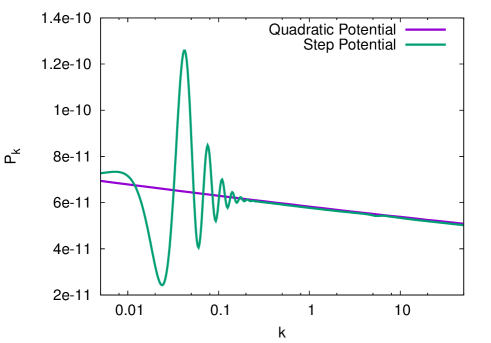
Figure 1: Power spectrum of scalar perturbations $P_{\zeta}(k)$ against momenta $k$ for quadratic potential and step potential with $c=0.002$, $d=0.02\;M_{pl}$ and $\phi_{s}=15.86\;M_{pl}$.

III.2 three-point function and Cesaro Sum

After numerically solving the background equations and the equation for scalar perturbations, we insert these solutions back into Eq. 18 to calculate the three-point function in momentum space. The three-point correlation function is numerically challenging task as it involves integrations that arise from equation (18). The integrands consist of three factors of $u_{k}$ or $u^{\prime}_{k}$ multiplied by the background factors of $a$, $\epsilon$ and $\eta$. The scalar perturbation function $u_{k}$ oscillates before horizon crossing at $\tau_{0}$, while after horizon it freezes out. Thus, the integration consists of two parts, before horizon crossing (BHC) part and after horizon crossing (AHC) part

$$\int_{-\infty}^{\tau_{end}}d\tau I(\tau)=\int_{-\infty}^{\tau_{0}}d\tau I(\tau)+\int_{\tau_{0}}^{\tau_{end}}d\tau I(\tau)$$ (35)

where $\tau_{0}$ is the horizon crossing point of the largest $k$ mode in the three-point correlation function and $I(\tau)$ is the integrand of the 3-point function given in Eq. 18 that contains background factors and product of three oscillating mode functions. The BHC and AHC parts of integration present different numerical challenges as the first has growing oscillations, as $\tau$ approaches negative infinity, while for the AHC part we have to regularize the three-point function by adding a total derivative term(Eq. 14) in the action. Without adding this term in the action, the AHC part of the integral is divergent as one of the term $a^{3}\epsilon\dot{\eta}\zeta^{2}\dot{\zeta}$ in the initial action grows as the scale factor Arroja ; Horner1 .

The contribution to the integral that arises from before horizon crossing poses significant technical challenges. In conformal time the initial big bag singularity is pushed back in conformal time to $\tau\rightarrow-\infty$. Thus, the scalar perturbations start deep inside the horizon and keep oscillating till horizon crossing point $\tau_{0}$ of the largest $k$ mode in the 3-point function. Now, there are different methods to numerically evaluate an oscillating integral over an infinite range. If we cutoff this infinite integral to some finite value, due to large oscillations this induces an spurious contribution of $O(1)$. Numerically it was shown that these kind of integrals can be evaluated by introducing an arbitrary damping factor into the integrand but this damping factor needs to be chosen carefullyXChen1 . Other techniques, such as boundary regularizaion, for evaluating such integrals are even more complex XChen3 ; Horner1 .

We have developed a different numerical technique, which is numerically more robust and elegant, using the Cesaro resummation of improper series. For oscillating integrand $I(\tau)$, the following expressions gives the definition of Cesaro integration

$$\int_{-\infty}^{\tau_{0}}d\tau I(\tau)\equiv\lim_{\tau\rightarrow-\infty}\frac{1}{\tau_{0}-\tau}\int_{\tau_{0}}^{\tau}d\tau^{\prime}\left(\int_{\tau_{0}}^{\tau^{\prime}}d\tau^{\prime\prime}I(\tau^{\prime\prime})\right)~{}.$$ (36)

This gives a specific definition to the improper integral on the left hand side whereas the right hand side is an average over the partial integrals that give convergent result for a wide range of improper integralscesa . However, we extended this method further and we defined a higher order Cesaro integral, with one additional average, to further improve the convergence as

$$\lim_{\tau\rightarrow-\infty}\frac{1}{\tau_{0}-\tau}\int_{\tau_{0}}^{\tau}d\tau^{\prime}\frac{1}{\tau_{0}-\tau^{\prime}}\int_{\tau_{0}}^{\tau^{\prime}}d\tau^{\prime\prime}\left(\int_{\tau_{0}}^{\tau^{\prime\prime}}d\tau^{\prime\prime\prime}I(\tau^{\prime\prime\prime})\right)~{}.$$ (37)

In our numerical program we have used this Cesaro integral with additional average Eq. (37) for faster convergence.

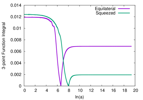
Figure 2: three-point correlation function, or generalized $f_{\textsc{NL}}$, integral plotted against the number of e-folds $N=\ln(a)$ for Equilateral and Squeezed triangles with horizon crossings at $6.5$ and $8$ e-folds. The generalized $f_{\textsc{NL}}$ is just the sum of the two asymptote(plateau) values at small and large e-folds corresponding to the two integrals in Eq 35.

This method quickly gives convergent results without introducing any artificial damping factors. This can be seen in Fig. 2 which shows the three-point function integral result plotted against the number of e-folds for an equilateral triangle and squeezed triangle cases. In this figure horizon crossings occur $\tau_{0}$ that corresponds to e-folds values of $6.5$ and $8$ for equilateral and squeezed triangle. This Fig 2 describe two different integration regimes BHC $\tau<\tau_{0}$ and AHC $\tau>\tau_{0}$. In BHC regime, we integrate in backward direction from the horizon crossing points using the Cesaro Integral Eq. 37. Our technique converges very quickly as can be seen that the integral plateaus as we go 5-6 e-folds before horizon crossing points. In the AHC regime, we integrate in the forward direction that also plateaus soon after horizon crossing. Thus, the three-point function integral, or generalized $f_{\textsc{NL}}$, is just the sum the two asymptote(plateau) values in the before and after horizon crossing regimes for each kind of triangle.

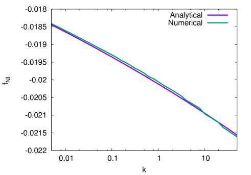
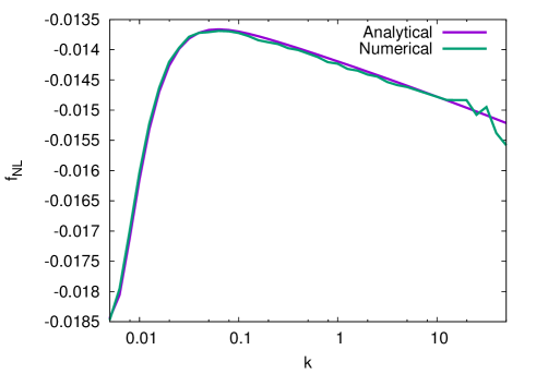
Figure 3: Numerical calculation of $f_{\textsc{NL}}$ for an equilateral triangle case($k=k_{1}=k_{2}=k_{3}$) alongside analytical result (Fig. a) for quadratic potential. Second plot show results for a squeezed triangle $k_{1}=0.005\;M_{pl}$ while $k=k_{2}=k_{3}$ are on the x-axis (Fig. b) for quadratic potential.

To test our procedure, we have calculated the three-point function numerically for $\frac{1}{2}m^{2}\phi^{2}$ potential and compared it with the corresponding analytical results given by Eq. 20. The numerical results when compared the analytical results are plotted in Fig. 3(a, b) for equilateral and squeezed triangles. As can be seen that our numerics follows very closely the analytical results for the quadratic potential. The Fig. 4 shows that our numerical technique is accurate to below one percent error for equilateral and squeezed triangles. In the extreme squeezed triangle limit $k\approx 5$ in Fig. 4 the errors are somewhat large as a compromise was made in the calculation due to the time and memory constraints.

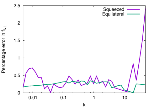
Figure 4: Percentage error in calculation of $f_{\textsc{NL}}$ for an equilateral triangle case when compared with analytical results plotted against $k=k_{1}=k_{2}=k_{3}$. While for squeezed triangle percentage error is plotted against $k=k_{2}=k_{3}$ while fixed $k_{1}=0.005\;M_{pl}$ for quadratic potential.

III.3 Application to Models with Significant Non-Gaussianity

Single field inflation with quadratic potential, $V(\phi)=\frac{1}{2}m^{2}\phi^{2}$, is categorized as chaotic inflation. The dynamics of inflation can be solved exactly in the slow roll limit for quadratic potential, thus we have used it as our base model for our study. However, it is was shown by Maldacena that single field slow roll models of inflation give rise to small non-Gaussianity of $O(\epsilon)$ as can seen in Fig. 3 and Eq. 20. In this paper we take the inflaton field mass to be $m=10^{-6}M_{p}$.

In single-field models of inflation significant non-Gaussianity can arise from different kinds of non trivial potentials, for example adding some features to quadratic potential. One such model consist of localized breaking of slow roll conditions. This can be achieved be adding a step in the quadratic potential as proposed by Adams

$$V_{step}(\phi)=\frac{1}{2}m^{2}\phi^{2}\left(1+c\tanh\frac{\phi-\phi_{s}}{d}\right).$$ (38)

where $c$ is the height of the step and $d$ the width of the step centred at $\phi_{s}$. This model has been used to improve the fit between LCDM and observed power spectrum and we have used the best fit parameters for the step potentialAdams . When inflation rolls down through this step it goes through a sharp acceleration in inflationary dynamics. The three-point correlation function is proportional to $\epsilon$ and $\eta$ parameters and deviation from slow roll gives rise to large interaction of modes near the step. This gives rise to large non-Gaussianity and generalized $f_{\textsc{NL}}\approx\frac{7c^{3/2}}{\epsilon d}$XChen1 . It important to mention here that $\epsilon$ does not change much by the step potential however $\eta\approx\frac{7c^{3/2}}{\epsilon d}$ gives dominant contribution to the 3-point function. Now, the three-point function integral Eq. 18 gets most of its contribution near the horizon crossing part of the modes. Thus, due to the step in the potential, the modes that cross the horizon near the step get a sharp kick that gives rise to large non-GaussianityXChen3 ; Amjad .

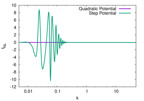
Figure 5: $f_{\textsc{NL}}$ for the step potential model plotted against $k=k_{1}=k_{2}=k_{3}$ for equilateral triangle case with step height and width given by $c=0.002$ and $d=0.02M_{pl}$ respectively while step is located at $\phi_{s}=15.86\;M_{pl}$.

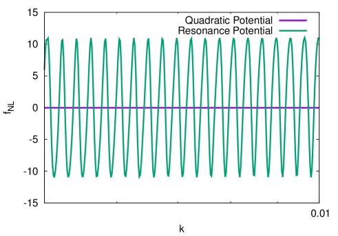
Figure 6: $f_{\textsc{NL}}$ for resonance model plotted against $k=k_{1}=k_{2}=k_{3}$ for equilateral triangle case for $c=5\times 10^{-7}$ and $0.0007$.

In Fig. 5 we present the calculation of $f_{\textsc{NL}}$ for equilateral triangle for the step potential model with parameters $c=0.002$, $d=0.02\;M_{pl}$ and $\phi_{s}=15.86\;M_{pl}$. The mode function $u_{k}$ that exits horizon at $\phi=\phi_{s}$ corresponds to $k_{s}\approx 0.01\;M_{pl}$. It is noted that peaks in $f_{\textsc{NL}}$ plot for the step potential are of $O(10)$ in amplitude that is about $500$ times the $f_{\textsc{NL}}$ of quadratic potential. However, if we move away from the step $k_{s}$, $k>0.5\;M_{pl}$ and $k<0.005\;M_{pl}$, the value of $f_{\textsc{NL}}$ for step potential tend to approach values for the quadratic potential.

The other kind of models that can give rise to large non-Gaussianity are models with global features in the potential like small oscillation on top of quadratic potential also know as Resonance modelXChen3

$$V_{res}(\phi)=\frac{1}{2}m^{2}\phi^{2}\left(1+c\sin(\phi/\Lambda)\right).$$ (39)

where $c$ is the amplitude of oscillation and $\Lambda$ is the frequency. In this model the non-Gaussianity is generated in the sub-horizon scales when modes are deep inside the horizon and they resonate, or interfere constructively, with the physical frequency $\omega\approx\frac{\dot{\phi}}{2\pi\Lambda}$. This model introduces a new scale $\Lambda$ into the quadratic potential as there small ripples in the entire plane of the potential. These ripples in the potential causes oscillation in $k$ space in the generalized $f_{\textsc{NL}}$ with amplitude $\frac{5c/4}{\Lambda^{2.5}\phi^{0.5}}$(see Fig. 6) while the power spectrum remains almost flat with tiny ripplesXChen3 . This kind of mechanism may be realized in brane inflation with duality cascadeBean ; Girma . Fig. 6 shows our computational technique works well for this kind of models as well.

IV Configuration Space Moments

Our goal is to develop a numerical technique for calculating the configuration space moments for perturbation $\zeta$ field in a general single-field model of inflation. For that we need to integrate three-point function in momentum space as given by Eqs. (25-27). As a starting point we shall consider slow roll models where these moments can be calculated analytically for the case of flat power spectrum $P_{k}^{\zeta}\approx const$ and then use the acquired insight to develop a general numerical procedure.

For instance, to calculate the $\left\langle\zeta^{3}(x)\right\rangle$, we substitute Eq. 19 into Eq. 25 to get

$$\left\langle\zeta^{3}\right\rangle=\int\prod_{i=1}^{3}\frac{dk_{i}^{3}}{k_{i}^{3}}\delta^{3}(\mathbf{k}_{1}+\mathbf{k}_{2}+\mathbf{k}_{3})\frac{(P_{k}^{\zeta})^{2}}{4\pi^{2}}\mathcal{A}_{\mathbf{k}_{1},\mathbf{k}_{2},\mathbf{k}_{3}}$$ (40)

where $\mathcal{A}$ is given by Eq. 20. For near flat spectra such integrals generally have both infrared and ultraviolet divergences, thus the correspondent moment is formally infinite. Ultraviolet divergences are regularized by the finite resolution of our measurements and should be studied in the context of a specific experiment. Infrared divergencies, on the other hand, seem of more conceptual nature since they come from contribution of the modes much larger than the observed Universe, which potentially reflect also less understood physics. To study them we introduce infrared $k_{min}$ and ultraviolet $k_{max}$ cutoffs and consider asymptotic behaviour as $z=k_{min}/k_{max}\to 0$. This procedure is somewhat ambiguous as to the order of imposing the cutoff and integrating over the $\delta$-function. This ambiguity does not, however, affect the coefficient of the leading infrared divergent term, which is, as we will see, what matters. It does affect subleading terms and this freedom can be used to minimize them in the numerical calculations. We suggest the procedure to use the $\delta$-function to eliminate in every term in the integral the least infrared divergent momentum and then integrate over the angles and the magnitudes of remaining two momenta in $k_{min}$ and $k_{max}$ limits.

Using the above mentioned procedure to evaluate the momentum space integrals, we also calculated the other two moments $\left\langle\zeta^{2}(x)\Delta\zeta(x)\right\rangle$, $\left\langle(\nabla\zeta(x))^{2}\Delta\zeta(x)\right\rangle$ by substituting Eq. 19 in to Eqs. 26 and 27. The asymptotic results are given below up to $z^{2}$ order

$$\left\langle\zeta^{3}(x)\right\rangle = (P_{k}^{\zeta})^{2}\left(\frac{3}{2}(\eta^{*}+2\epsilon^{*})\ln^{2}(z)-3\epsilon\ln(z)+\epsilon\left(15-24\ln(2)\right)+O(z^{2})\right),\quad$$ (41)

$$\left\langle\zeta^{2}(x)\Delta\zeta(x)\right\rangle = -(P_{k}^{\zeta})^{2}k_{max}^{2}\left((\eta^{*}+2\epsilon^{*})\ln(z)-\frac{\epsilon^{*}}{6}\left(\pi^{2}-28+32\ln(2)\right)+\mathcal{O}(z^{2})\right),$$ (42)

$$\left\langle(\nabla\zeta(x))^{2}\Delta\zeta(x)\right\rangle = -(P_{k}^{\zeta})^{2}k_{max}^{4}\left(\frac{1}{6}\eta^{*}+\epsilon^{*}\left(\frac{4}{3}\ln(2)-\frac{527}{900}\right)+O(z^{2})\right).$$ (43)

Evidently, the first two moments are divergent in $z\rightarrow 0$ limit, $\left\langle\zeta^{3}(x)\right\rangle\propto\ln^{2}(z)$ while $\left\langle\zeta^{2}(x)\Delta\zeta(x)\right\rangle\propto\ln(z)$. The modified regularization sequence retains the coefficients in the divergent terms but changes the constant ones. Here we note that the last moment with the most derivatives $\left\langle(\nabla\zeta(x))^{2}\Delta\zeta(x)\right\rangle$ is finite as $z\to 0$ and thus remains sensitive to regularization details.

Now, if we look at the expression for Euler characteristic (Eq. 3) or any other observables, the configuration space moments are always dividedPogosyan1 by the variances $\sigma^{2}$ and $\sigma_{1}^{2}$ given in Eqs. 45.

$$\sigma^{2}=\left\langle\zeta^{2}(x)\right\rangle=P_{k}^{\zeta}\ln\left(\frac{k_{max}}{k_{min}}\right)\quad$$ (44)

$$\sigma_{1}^{2}=\left\langle(\nabla\zeta(x))^{2}\right\rangle=P_{k}^{\zeta}\frac{k^{2}_{max}-k^{2}_{min}}{2}~{}.$$ (45)

Thus, even though the moments by themselves are divergent, the observed quantities are finite. Normalized or scaled by these variances the moments to leading order in slow roll are given by

$$S_{3} \equiv \frac{\left\langle\zeta^{3}(x)\right\rangle}{\sigma^{4}}\simeq\frac{3}{2}(\eta^{*}+2\epsilon^{*}),\quad$$ (46)

$$T_{3} \equiv \frac{\left\langle\zeta^{2}(x)\Delta\zeta(x)\right\rangle}{\sigma^{2}\sigma_{1}^{2}}\simeq-2(\eta^{*}+2\epsilon^{*}),$$ (47)

$$U_{3} \equiv \frac{\left\langle(\nabla\zeta(x))^{2}\Delta\zeta(x)\right\rangle}{\sigma_{1}^{4}}$$ (48)

$$\simeq -\frac{2}{3}\left(\eta^{*}+\epsilon^{*}\left(8\ln(2)-\frac{527}{150}\right)\right).$$

Note that the numerical coefficient in front of $\epsilon^{*}$ in $U_{3}$ is also equal to two with better than $2\%$ accuracy, thus all three normalized moments are determined by $\eta^{*}+2\epsilon^{*}$. From the above moments, we have found that the local non-Gaussianity parameter for single-field slow roll inflation is $f_{\textsc{NL}}=-\frac{5}{12}(\eta^{*}+2\epsilon^{*})$ which is independent of the shape and scale of the triangles.

For numerical calculation of momentum space integrals finite momentum space cutoff is unavoidable. The above analytical results guide us to the following numerical procedure for the general single-field model. We calculate the moments using the exact result of 3-point function Eq. 18, with the triangularity condition $\mathbb{k}_{1}+\mathbb{k}_{2}+\mathbb{k}_{3}=0$ applied to the least divergent momentum.To numerically obtain $z\to 0$ result we integrate the remaining two momenta in finite range $[k_{min}$,$k_{max}]$, then vary $\frac{k_{min}}{k_{max}}$ and find the asymptotic limit (plateau value) for the scaled moments $S_{3}$, $T_{3}$ and $U_{3}$. Procedure we follow is that we fix $k_{min}=0.005\;M_{pl}$ that corresponds to the mode that inflates $64$ e-folds after horizon crossing that is roughly the largest scales of the observed Universe and vary $k_{max}$ or $z$. As seen in Fig. 7, for quadratic potential the numerical calculation of $S_{3}$, $T_{3}$ and $U_{3}$ gives very stable result already by $k_{max}\approx 0.1\;M_{pl}$.

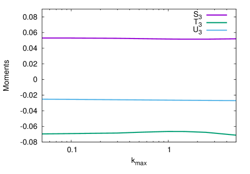
Figure 7: Moments plotted against $k_{max}$ with fixed $k_{min}=0.005\;M_{pl}$ for quadratic potential.

This fast convergence reflects smallness of the constant terms in Eqs. 41 and 42, $-1.6\epsilon$ and $0.8\epsilon$ correspondingly. Slight drop in values of moments in Fig. 7 is a numerical artifact as higher values of $k_{max}>2M_{pl}$ require very fine resolution $\Delta k$ in momenta integrations.

Thus we see that the infrared divergences for near flat spectra can be dealt with very efficiently during numerical momenta integration. It is sufficient to integrate over just a decade of wave-numbers to obtain a good approximation to the asymptotic values. The quadratic potential gives the values $S_{3}=0.0517$, $T_{3}=-0.0664$ and $U_{3}=-0.0264$ with at most $5\%$ error in the calculation of these moments.

For potential with features such as step potential, the answer for the moments depends on the range of k-integration in relation to the modes that give additional contribution to non-Gaussian signal. For the step potential, as Fig. 5 demonstrates, the support for correction to the $f_{\textsc{NL}}$ is finite, encompassing the range from $k\approx 0.01\;M_{pl}$ to $k\approx 0.2\;M_{pl}$ for the parameters used there. Fig. 8 shows the change in the moments if we fix $k_{min}=0.005\;M_{pl}$ but vary $k_{max}$.

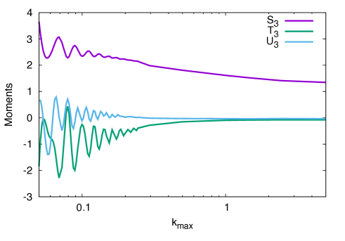
Figure 8: Moments plotted against $k_{max}$ with fixed $k_{min}=0.005\;M_{pl}$ for step potential with $c=0.002$, $d=0.02\;M_{pl}$ and $\phi_{s}=15.86\;M_{pl}$.

The asymptotic behaviour can be understood from the following consideration. Let us write

$$S_{3}^{step}(k_{min},k_{max})=S_{3}^{quad}+\frac{\Delta\left\langle\zeta^{3}\right\rangle}{\sigma^{4}(k_{min},k_{max})},$$ (49)

and correspondingly for the other moments, where $\Delta\left\langle\zeta^{3}\right\rangle$ signifies additional contribution to the momentum integral above the baseline quadratic values. In such a split the first term, $S_{3}^{quad}$ is practically independent on the $k_{min}$ or $k_{max}$, as we discussed above. The second correction term depends on the integration range. As soon as this range encompasses the support for the extra non-Gaussian contribution, it starts decreasing as the correspondent powers of the variances, i.e. as $1/\sigma^{4}\approx\ln^{-2}(k_{max}/k_{min})$ for $S_{3}$, $1/(\sigma^{2}\sigma_{1}^{2})\approx k_{max}^{-2}\ln^{-1}(k_{max}/k_{min})$ for $T_{3}$ and $1/\sigma_{1}^{4}\approx k_{max}^{-4}$ for $U_{3}$. This explains the quick convergens of $T_{3}$ and $U_{3}$ moments to their baseline values as $k_{max}>1\;M_{pl}$ and slow logarithimic decrease of $S_{3}$ exhibited in Fig. 8.

In cosmological applications the $k_{min}$ to $k_{max}$ range depends on observational setup or analysis choice. For large-scale structure studies the ratio of largest observable scale $\sim 10\;Gpc$ to the smallest presently mildly non-linear scale $\sim 10\;Mpc$ is of order of a thousand, which points to $k_{max}\sim 5\;M_{pl}$. This is the value that we adopt in the following sample calculations.

For the step potential we plot the moments against the parameters $c$ and $d$ as displayed in Figs. 9 and 10. The limit of the quadratic potential is reached as $c\to 0$ or $d\to\infty$. It can be seen that the magnitude of $S_{3}$ moment increases significantly as the height of the step $c$ increases (Fig 9) or the width $d$ decreases (Fig. 10). At the same time, the moments $T_{3}$ and $U_{3}$ remain practically unchanged from their small values in quadratic potential limit, as expected from our analysis of $k_{max}$ behaviour. The first moment $S_{3}$ is plotted against $c$ and $d$ in Fig. 11 which shows that sharper the step, smaller width and higher step, the higher the moment.

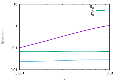
Figure 9: Absolute values of the moments for the step potential plotted against parameter $c$ for fixed $d=0.01\;M_{pl}$.

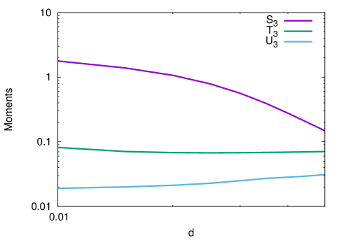
Figure 10: Absolute values of the moments for the step potential plotted against parameter $d$ for fixed $c=0.01$.

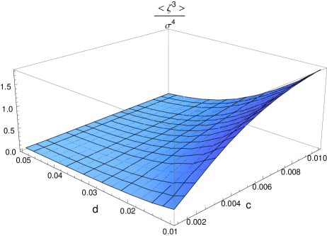
Figure 11: Moment $S_{3}=\frac{\left\langle\zeta^{3}\right\rangle}{\sigma^{4}}$ for the step potential plotted against parameters $c$ and $d$ showing that this moment peeks when the step is sharpest.

V Geometrical Statistics and Minkowski Functionals

Many geometrical statistics, including Minkowski functionals, of the mildly non-Gaussian fields can be expressed as series expansion in higher-order moments of the field and its derivatives with powers of $\sigma$ controlling the expansion order PGP09 . First order non-Gaussian corrections are linear in $\sigma$ and defined by cubic normalized moments that we have studied earlier. For the models with nearly flat power spectrum that we consider, we adopt the value of the variance $\sigma\approx\sqrt{P_{\zeta}\ln(k_{max}/k_{min})}\approx 1.2\times 10^{-4}$ with $P_{\zeta}=2.2\times 10^{-9}$ suggested by Planck data planck2 and $k_{max}/k_{min}=10^{3}$.

The simplest geometrical statistic or Minkowski functional is the filling factor $f_{V}=\int_{\nu\sigma}^{\infty}d\zeta P(\zeta)$, i.e. the fraction of volume above the threshold $\nu$. Its moment expansion gives

$$f_{V}(\nu)=\frac{1}{2}\mathrm{Erfc}\left(\frac{\nu}{\sqrt{2}}\right)+\frac{e^{-\frac{\nu^{2}}{2}}}{\sqrt{2\pi}}\sigma H_{2}(\nu)\frac{S_{3}}{6}+O(\sigma^{2}).$$ (50)

The first non-Gaussian correction only depends on $S_{3}$ multiplied by Hermite polynomial of order two. Thus, linear in $\sigma$ non-Gaussian part of $f_{V}(\nu)$ has a global shape that is independent of any model while its magnitude will depend on the magnitude of moment $S_{3}$. Thus for the step potential, the filling factor can be as large as $500$ times the $f_{V}$ for quadratic potential. In Fig. 12 a single curve shows the non-Gaussian part of the filling factor both for the model with quadratic potential with $f_{V}$ correction of order $\mathcal{O}(10^{-7})$ (as labeled on the left vertical axis) and for the step potential for which it is $\mathcal{O}(10^{-5})$ (the right vertical axis).

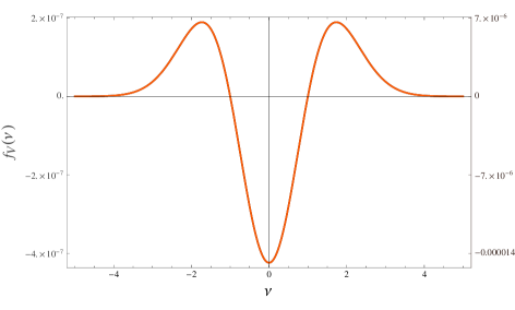
Figure 12: Non gaussian part of filling factor $f_{V}$ as the function of threshold $\nu$. Values on the left vertical axis are for quadratic potential while values on the right axis are for step potential with $c=0.01$ and $d=0.01\;M_{pl}$.

There are several advantages to use the value of the filling factor $f_{V}$ instead of $\nu$ as a variable in which to express all other statistics. Indeed, the fraction of volume occupied by a data set is often available even from the limited data, whereas specifying $\nu$ requires prior knowledge of the variance $\sigma$ which may not be easily obtainable. In some cases non-Gaussian analysis itself gives more robust way to determine the variance. Following Matsubara2 we introduce the effective threshold $\nu_{f}\equiv\sqrt{2}\mathrm{Erfc}^{-1}(2f_{V})$ be used as an observable alternative to $\nu$. To the first order correction in $\sigma$ we have the relation

$$\nu=\nu_{f}+\sigma\frac{S_{3}}{6}H_{2}(\nu_{f}).$$ (51)

Another Minkowski functional in 3D is the area (per unit volume) of isodensity contours $\mathcal{N}_{3}(\nu)$. Up to first non-Gaussian contribution, this quantity is expressed in terms of third-order moments as

$$\mathcal{N}_{3}(\nu)\approx\frac{2e^{-\frac{\nu^{2}}{2}}\sigma_{1}}{\sqrt{3}\pi\sigma}\Bigg{[}1+\sigma\left(\frac{S_{3}}{6}H_{3}(\nu)+\frac{T_{3}}{2}H_{1}(\nu)\right)\Bigg{]},~{}$$ (52)

depending on moments $S_{3}$ and $T_{3}$. In Fig. 13 we show the non-Gaussian $\mathcal{N}_{3}(\nu)$ for quadratic and step potential. Besides vastly different amplitudes, it exhibits different shape that distinguishes the two models. For quadratic potential $H_{3}$ contribution is small and $\mathcal{N}_{3}$ has just two measurable extrema with small secondary ones near the edges, while due to the large value of $S_{3}$ the $H_{3}$ part is prominent for the step potential, giving rise to four distinct extrema, as seen in Fig. 13.

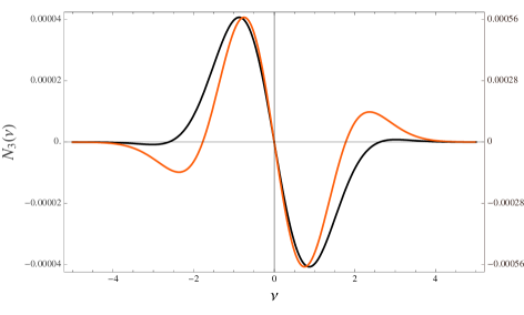
Figure 13: Non gaussian part of area of isodensity contours $\mathcal{N}_{3}(\nu)$ for quadratic potential in black with values on left vertical axis as a function of threshold $\nu$. Similarly, $\mathcal{N}_{3}(\nu)$ for step potential, for $c=0.01$ and $d=0.01\;M_{pl}$, is show in red(lighter colour) with values on right vertical axis as a function of threshold $\nu$.

As a function of $\nu_{f}$, i.e of the filling factor, the area of isodensity contours is

$$\mathcal{N}_{3}(\nu_{f})\approx\frac{2e^{-\frac{\nu_{f}^{2}}{2}}\sigma_{1}}{\sqrt{3}\pi\sigma}\Bigg{[}1-\sigma\left(S_{3}+\frac{T_{3}}{4}\right)H_{1}(\nu_{f})\Bigg{]},\quad$$ (53)

which demonstrates the general outcome of eliminating the highest order Hermite polynomial term when switching from $\nu$ to $\nu_{f}$. Because of that, in Fig. 14, the area of isodensity contours $\mathcal{N}_{3}(\nu_{f})$ has a model independent shape that is proportional to $e^{-\frac{\nu_{f}^{2}}{2}}H_{1}(\nu_{f})$. The $\mathcal{N}_{3}(\nu_{f})$ for the step potential has values of order $10^{-3}$ on right axis while for quadratic potential it has values of order $10^{-5}$ on the left axis.

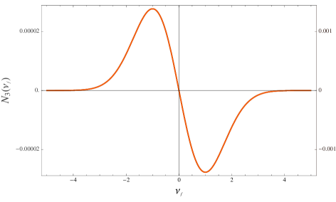
Figure 14: Non gaussian part of area of isodensity contours $\mathcal{N}_{3}(\nu_{f})$ for quadratic potential in black with values on left vertical axis as a function of filling factor $\nu_{f}$. Similarly, $\mathcal{N}_{3}(\nu_{f})$ for step potential, for $c=0.01$ and $d=0.01\;M_{pl}$, in red(lighter colour) with values on right vertical axis as a function of filling factor $\nu_{f}$.

An important Minkowski functional in cosmology is the Euler characteristic (or genus) that is used to characterize the topology of the isocontours of random fields. The definition generally used by cosmologists is that the genus is the number of holes minus the number of isolated regions above a threshold $\nu$ in a random field (thus, for one isolated region, the genus is just the number of holes minus one), while Euler characteristic of the excursion set is just minus genus, see Eq. 3. Euler characteristic density can be also considered as a function of filling-factor-deduced threshold $\nu_{f}$ rather than the threshold $\nu$.

$$\chi_{\textsc{3D}}(\nu_{f})\approx\frac{1}{(2\pi)^{2}}\left(\frac{\sigma_{1}}{\sqrt{3}\sigma}\right)^{3}e^{-\nu_{f}^{2}/2}\Bigg{[}H_{2}(\nu_{f})-\Bigg{.}$$

$$\Bigg{.}\sigma\left(S_{3}+\frac{3}{4}T_{3}\right)H_{3}(\nu_{f})-\sigma\left(S_{3}+\frac{9}{4}U_{3}\right)H_{1}(\nu_{f})\Bigg{]}\quad$$ (54)

We have calculated Euler characteristic $\chi_{\textsc{3D}}$ of the 3D perturbation field $\zeta$ for two models of inflation, the quadratic inflation and step potential model. For quadratic potential, the non-Gaussian part of $\chi_{\textsc{3D}}$ as a function of threshold $\nu$ is plotted in Fig. 15.

Figure 15: Non gaussian part of Euler characteristic $\chi_{\textsc{3D}}$ as a function of threshold $\nu$ for the quadratic potential. The shaded region shows the error bars coming from the error in calculation of moments that are roughly $5$ percent.

showing the small amplitude of the non-Gaussianity of order $10^{-7}$ and the presence of all three $H_{1},H_{3},H_{5}$ harmonics. Euler characteristic as a function of $\nu_{f}$ is given in Fig. 16.

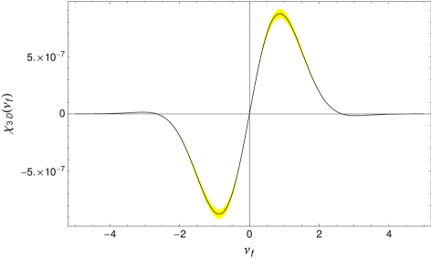
Figure 16: Non gaussian part of genus as a function of filling factor $\nu_{f}$ for the quadratic potential. The shaded region shows the error bars coming from the error in calculation of moments that are roughly $5$ percent.

For the quadratic inflation $S_{3}+3T_{3}/4\approx 0.002$ is notably smaller than $S_{3}+9U_{3}/4\approx-0.008$, hence the result is dominated by the $H_{1}$ term that has only one zero crossing at origin as can be seen in Fig. 16.

While the $\mathcal{O}(10^{-7})$ non-Gaussian correction to Euler characteristic for the quadratic potentialis small, as expected, and is hardly observable, for the step potential, it will have the magnitude $10$ to $500$ times larger. Fig. 17 shows $\chi_{\textsc{3D}}(\nu)$ curves for two different sets of $c$ and $d$ parameters, with magnitude of the effect differing by an order of magnitude, namely $\mathcal{O}(10^{-5})$ for $c=0.0018$ and $d=0.022\;M_{pl}$ and $\mathcal{O}(10^{-4})$ for $c=0.01$ and $d=0.01\;M_{pl}$. At the same time the shapes of the Euler characteristic curves are very similar dominated by $S_{3}H_{5}(\nu)$ term.

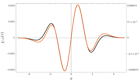
Figure 17: Non gaussian part of genus as a function of threshold $\nu$ for the step potential for two parameter sets ($c=0.0018$, $d=0.022\;M_{pl}$ in black on left axis) and ($c=0.01$, $d=0.01\;M_{pl}$ in red, lighter colour, on right axis).

This can be seen explicitly also when measuring Euler characteristic as a function of $\nu_{f}$ as shown in Fig. 18.

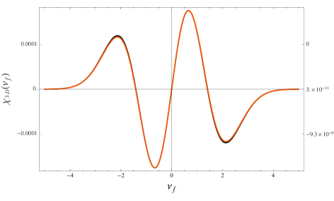
Figure 18: Non gaussian part of genus as a function of filling factor $\nu_{f}$ for the step potential for two parameter sets ($c=0.0018$, $d=0.022\;M_{pl}$ in black on left axis) and ($c=0.01$, $d=0.01\;M_{pl}$ in red, lighter colour, on right axis).

With $S_{3}$ dominant for all the values of step parameters $c$ and $d$ studied, the non-Gaussian part of Euler characteristic exhibits a universal form $\chi_{\textsc{3D}}\propto\sigma S_{3}\left(H_{1}(\nu_{f})+H_{3}(\nu_{f})\right)$ that is a distinguishing signature of this particular model of non-Gaussianity.

VI Results and Discussion

The main goal in this paper was to develop theoretical formalism that links early Universe inflationary models to the observable geometrical characteristics of the initial field of scalar adiabatic cosmological perturbations. The link to non-Gaussian features in such statistics as Minkowski functionals, extrema counts, and skeleton properties is provided by studying the higher order moments of the perturbation field and its derivatives in configuration space.

We have investigated from the first principles the third-order configuration space moments that give first non-Gaussian corrections. To calculate these moments we have to calculate the three-point bispectrum in momentum space and then integrate over the three momenta with appropriate combinations of derivative operators.

We presented a complete prescription for the calculation of three-point function, in momentum space, for general single-field models of inflation, improving on the computational procedures used in the previous literature. We have devised a method to precisely calculate the required time integral over products of perturbation mode functions in “before horizon crossing” as well as in “after horizon crossing” regimes. For that we stressed the necessity to use the action that gives stable three-point function integral result till the very end of inflation Arroja and we developed novel technique using modified Cesaro summation to integrate the highly oscillatory “before horizon crossing” part of the three-point function integral. Thus, we calculated the bispectrum in terms of generalized $f_{\textsc{NL}}$ that even works for models that break slow roll conditions and where there is significant variation in slow roll parameters.

In the configuration space we have studied infrared and ultraviolet divergences of the third-order perturbation moments. Analytical analysis of the slow-roll models allowed us to illuminate the role of the dominant infrared divergent logarithms in the moment calculations. These terms determine observable moments scaled by the appropriate powers of the variance of the field or its derivative. The moments that do not contain infrared divergence are found to be sensitive to ultraviolet smoothing prescription. We implemented this understanding in numerical procedure that transforms bispectrum results to the configuration space moments.

To calculate the moments we had to integrate out triangles of all shapes and sizes. We introduced the regularization in the momentum space integrals with both infrared $k_{min}$ and ultraviolet $k_{max}$ cuts. We observed that for the basic flat spectrum these moments do not depend on $k_{min}$, instead leading logarithmic terms depend on the ratio $z=\frac{k_{min}}{k_{max}}$ of the smallest the largest scales and can be robustly select relative to subdominant term by varying this ratio which is numerically easier to do by varying $k_{max}$. It was further noted that these moments divided by their corresponding variances are finite quantities and they reach a plateau for large values of $k_{max}$ hence they are also independent of physics of the smallest scales (see Figs. 7 and 8). For the step potential it was shown that the moment $S_{3}$ is the one that is affected the most while the other two moments $T_{3}$ and $U_{3}$ are very mildly affected by the step if the range of $k$ integration encompasses all the modes with enhanced non-Gaussian response.

The Minkowski functionals of the cosmological perturbation field generated on inflation depend on the balance between the moments of the field and its derivatives up to the second order. We have demonstrated typical behaviour of the non-Gaussian corrections to several Minkowski functionals of $\zeta$ field in the slow-roll quadratic model and the model with step potential. Such corrections show different signatures for different models of inflation. In particular step potential, as representative of the class of models with enhanced non-Gaussian response over limited wavelength range, leads to a characteristic universal form of the genus curve as function of the filling factor if measurements include a sufficiently large interval of scales.

VII Acknoledgements

This research has been supported by Natural Sciences and Engineering Research Council (NSERC) of Canada Discovery Grant. The computations were performed on the SciNet HPC Consortium. SciNet is funded by: the Canada Foundation for Innovation under the auspices of Compute Canada; the Government of Ontario; Ontario Research Fund - Research Excellence; and the University of TorontoSciNet .

References

- [1] W. C. Jones et al. A measurement of the angular power spectrum of the cmb temperature anisotropy from the 2003 flight of boomerang. ApJ, (astro-ph/0507494), 2005.
- [2] S. Hanany et al. Maxima-1: A measurement of the cosmic microwave background anisotropy on angular scales of 10 arcminutes to 5 degrees. Astrophys., J.(545):L5, 2000.
- [3] J. L. Sievers et al. Cosmological results from five years of 30 ghz cmb intensity measurements with the cosmic background imager. arXiv:0901.4540.
- [4] C. L. Reichardt et al. High resolution cmb power spectrum from the complete acbar data set. Astrophysical Journal, (694):1200–1219, 2009.
- [5] C. L. Bennett. Nine-year wilkinson microwave anisotropy probe (wmap) observations: Final maps and results. Astrophys.J.Suppl., 208:20, 2013.
- [6] P.A.R. Ade et al. Planck 2013 results. i. overview of products and scientific results. Astron.Astrophys., 571:A1, 2014.
- [7] P. A. R. Ade et al. Planck 2013 results. xxiii. isotropy and statistics of the cmb. arXiv:1303.5083 [astro-ph.CO].
- [8] P.A.R. Ade et al. Planck 2013 results. XVI. Cosmological parameters. Astron.Astrophys., 571:A16, 2014.
- [9] P.A.R. Ade et al. Planck 2015 results. xx. constraints on inflation. 2015.
- [10] Alan H. Guth. Inflationary universe: A possible solution to the horizon and flatness problems. D(23):347, 1981.
- [11] A. H. Guth and S. Y. Pi. Physical Review Letters, (49):1110, 1982.
- [12] A. D. Linde. Physics Letters, B(108):389, 1982.
- [13] V. F. Mukhanov and G. Chibisov. JETP Letters, (33):532, 1981.
- [14] James M. Bardeen, Paul J. Steinhardt, and Michael S. Turner. Spontaneous Creation of Almost Scale - Free Density Perturbations in an Inflationary Universe. Phys.Rev., D28:679, 1983.
- [15] A. A. Starobinskii. The Perturbation Spectrum Evolving from a Nonsingular Initially De-Sitter Cosmology and the Microwave Background Anisotropy. Soviet Astronomy Letters, 9:302–304, June 1983.
- [16] Viatcheslav Mukhanov. Physical Foundations of Cosmology. Cambridge University Press, 1st edition, 2005.
- [17] A. D. Linde. Particle Physics and Inflationary Cosmology. Harwood, Chur, Switzerland, 1990, hep-th/0503195 edition, 2005.
- [18] Andrei D. Linde. Inflationary Cosmology. Lect.Notes Phys., 738:1–54, 2008.
- [19] Lev Kofman, Andrei Linde, and V. Mukhanov. Inflationary theory and alternative cosmology. JHEP, 10(057), 2002.
- [20] J. M. Maldacena. Non-gaussian features of primordial fluctuations in single field inflationary models. JHEP, 05:013, 2003.
- [21] Takahiko Matsubara. Analytic expression of the genus in a weakly non-gaussian field induced by gravity. Astrophysical Journal, Part 2 - Letters, 434(2):L43–L46, 1994.
- [22] J. M. Bardeen, J. R. Bond, N. Kaiser, and A. S. Szalay. The statistics of peaks of gaussian random fields. Astrophysical Journal, Part 1, 304:15–61, May 1986.
- [23] D. Pogosyan, C. Gay, and C. Pichon. Invariant joint distribution of a stationary random field and its derivatives: Euler characteristic and critical point counts in 2 and 3D. Phys. Rev. D, 80(8):081301, 2009.
- [24] D. Pogosyan, C. Pichon, and C. Gay. Non-gaussian extrema counts for cmb maps. PRD, 84(8):083510, October 2011.
- [25] Christophe Gay, Christophe Pichon, and Dmitry Pogosyan. Non-Gaussian statistics of critical sets in 2 and 3D: Peaks, voids, saddles, genus and skeleton. Phys.Rev., D85:023011, 2012.
- [26] S. Codis, C. Pichon, D. Pogosyan, F. Bernardeau, and T. Matsubara. Non-Gaussian Minkowski functionals and extrema counts in redshift space. 435:531–564, October 2013.
- [27] Daniel Baumann. Tasi lectures on inflation. TASI Lectures, 2009.
- [28] V. F. Mukhanov. JETP Lett., (41):493, 1985.
- [29] David Seery and J. E. Lidsey. Primordial non-gaussianities in single field inflation. 2005.
- [30] Frederico Arroja and Takahiro Tanaka. A note on the role of the boundary terms for the non-Gaussianity in general k-inflation. JCAP, 1105:005, 2011.
- [31] Jonathan S. Horner and Carlo R. Contaldi. Non-Gaussian signatures of general inflationary trajectories. JCAP, 1409:001, 2014.
- [32] Clare Burrage, Raquel H. Ribeiro, and David Seery. Large slow-roll corrections to the bispectrum of noncanonical inflation. JCAP, 1107:032, 2011.
- [33] N. Bartolo, S. Matarrese E. Komatsu, and A. Riotto. Phys. Rept., 402:103, 2004.
- [34] J. Richard Gott, Wesley N. Colley, Chan-Gyung Park, Changbom Park, and Charles Mugnolo. Genus topology of the cosmic microwave background from the wmap 3-year data. Royal Astronomical Society, 377:1668, 2007.
- [35] Changbom Park, Yun-Young Choi, Michael Vogeley, J. Richard Gott III, Juhan Kim, Chiaki Hikage, Takahiko Matsubara, Myeong-Gu Park, Yasushi Suto, David H. Weinberg, and SDSS collaboration. Topology analysis of the sloan digital sky survey: I. scale and luminosity dependences.
- [36] Xingang Chen et al. Large non-gaussianities in single field inflation. JCAP, 0706(023), 2007.
- [37] Xingang Chen, Richard Easther, and Eugene A. Lim. Generation and characterization of large non-gaussianities in single field inflation. 01 2008.
- [38] E. Cesàro. Bull. Sci. Math., 14(1):114–120, 1890.
- [39] Jennifer Adams, Bevan Cresswell, and Richard Easther. Inflationary perturbations from a potential with a step. Phys. Rev. D, 64:123514, Nov 2001.
- [40] Amjad Ashoorioon, Axel Krause, and Krzysztof Turzynski. Energy transfer in multi field inflation and cosmological perturbations. 10 2008.
- [41] Rachel Bean, Xingang Chen, Girma Hailu, S.-H. Henry Tye, and Jiajun Xu. Duality cascade in brane inflation. 02 2008.
- [42] Girma Hailu and S. H. Henry Tye. Structures in the gauge/gravity duality cascade.
- [43] T. Matsubara. Statistics of smoothed cosmic fields in perturbation theory. i. formulation and useful formulae in second-order perturbation theory. ApJ, 584(1), 2003.
- [44] Chris Loken et al. Scinet: Lessons learned from building a power-efficient top-20 system and data centre. J. Phys., Conf. Ser.(256 012026), 2010.