Vacuum fluctuation inside a star and their consequences for neutron stars, a simple model

Abstract

Applying semi-classical Quantum Mechanics, the vacuum fluctuations within a star are determined, assuming a constant mass density and applying a monopole approximation. It is found that the density for the vacuum fluctuations does not only depend linearly on the mass density, as assumed in a former publication, where neutron stars up to 6 solar masses were obtained. This is used to propose a simple model on the dependence of the dark energy to the mass density, as a function of the radial distance $r$. It is shown that stars with up to 200 solar masses can, in principle, be obtained. Though, we use a simple model, it shows that in the presence of vacuum fluctuations stars with large masses can be stabilized and probably stars up to any mass can exist, which usually are identified as black holes.

1 Introduction

The theory of General Relativity (GR) [1] has passed up to now all observational tests. However, all these tests are for weak gravitational fields [2] (to which we also count the gravitational field in the Hulse-Taylor pulsar [3]), compared to the field strength near the Schwarzschild radius.

The standard GR predicts singularities, due to the black-hole solution. This solution has a singularity in the center and a coordinate singularity called the event horizon. No information below this event horizon can reach an external observer, even nearby.

In our philosophical understanding, no theory should have a singularity, not even a coordinate singularity of the type discussed above. The appearance of a singularity hints to the incompleteness of a theory. While this is generally accepted for the singularity at the center, the discussion is going on whether this also applies for the coordinate singularity.

In recent publications [4, 5] an algebraic extension of GR to pseudo-complex (pc) coordinates was proposed, denoted as pseudo-complex General Relativity (pc-GR). The pc-coordinates have the structure $X^{\mu}=x^{\mu}+Iy^{\mu}$, with $I^{2}=1$. Due to the property of $I^{2}=1$, variables with $x^{\mu}=\pm y^{\mu}$ have no inverse, thus the pc-variables form not a field but a ring. The absolute value squared $\mid X^{\mu}\mid$ = $X^{\mu*}X^{\mu}$ of these variables, with $X^{\mu*}=x^{\mu}-Iy^{\mu}$, are zero, though the variables themselves are different from zero. A modified variational principle was proposed, which states that the variation of the action, which is now pseudo-complex, has to be proportional to a function whose absolute value is zero, called also a generalized zero. As a consequence, the Einstein equations change and, in the limit of $y^{\mu}=0$, have the form

$$G_{\mu\nu} = -8\pi T^{\Lambda}_{\mu\nu}~{}~{}~{},$$ (1)

where the the gravitational constant and the velocity of light were set to 1. The $T^{\Lambda}_{\mu\nu}$ is the energy momentum tensor of the dark energy and the index $\Lambda$ denotes this association. The same equation is obtained, adding in the standard GR by hand an energy-momentum tensor on the right hand side of the Einstein equations.

Using semi-classical Quantum Mechanics (QM), where the background metric is fixed, it was shown that a mass changes the vacuum structure in its vicinity. The fluctuations increase toward the Schwarzschild radius and become infinite there [6].

Because a quantized theory of gravitation does not exist yet, one relies on semi-classical QM, which does not permit to include the back-reaction of the vacuum fluctuation in a consistent way and is not applicable for strong gravitational fields. Therefore, we proceeded to assume the presence of vacuum fluctuations, proposing a radial dependence such that for large distances, compared to the Schwarzschild radius, the corrections to standard GR can not be measured yet. For the dark energy a fluid model was chosen, leading to corrections of the metric in the order of $1/r^{3}$. (In [7] other radial dependencies were investigated with similar qualitative results). This did permit to include the back-reaction to the metric and to solve the Einstein equations.

The procedure reflects a general principle, namely: Mass not only curves the space but also modifies the vacuum structure, such that the metric itself changes. Because we used a fluid model, an additional parameter $B=bm^{3}$ was introduced, where $m$ is the mass in units of length and $b$ is the actual parameter, measuring the coupling between the central mass to the vacuum fluctuations outside the star. By an adequate choice of this parameter, namely that $g_{00}$ satisfies $\left(1-\frac{2m}{r}+\frac{B}{2r^{3}}\right)$ $>$ 0, the $b$ obtains a lower bound, such that there is no event horizon!

In [7] the consequences for the case of the Kerr-solution were investigated. It was shown that the orbital frequency of particles in a circular orbit exhibit a maximum in the frequency which from there on is decreasing again toward lower radial distances.

Observing Quasi Periodic Objects (QPO) in the accretion disk of galactic black holes [8, 9, 10, 11], assuming that they correspond to local bright spots in the disk following its orbital motion, one can deduce a radial distance using the prediction of the theory (GR or pc-GR). Measuring at the same time the redshift, using $K-\alpha$ lines, also has as a result a given radial distance. For a consistent theory, in both measurements the deduced radial distances have to be the same. And here is the problem: They agree in pc-GR but not in GR [12]. There is still a discussion going on if the QPO follows the orbital motion of the disk or are due to oscillations within the disk [13] provoked by the stellar partner, which would change the conclusions. Our argument that the QPO’s in accretions disks around galactic black holes correspond to local bright spots, following the motion of the disk, is based on their observation in the accretion disks around large masses in the center of galaxies, with no stellar partner nearby, and that the physics in both should be very similar.

Another prediction of pc-GR is that the accretion disk appears brighter and exhibits a dark ring [14]. A model of a thin, infinitely extended disk [15] was applied. This dark ring is due to the maximum of the orbital frequency of particles in a circular orbit. At the maximum shear forces between particles in two neighboring orbits is small and thus little heat is additionally created.

As one notes, pc-GR provides definite observable predictions, which will be observed in near future.

A further application of pc-GR is given in [16], where the question was investigated if due to the presence of dark energy, neutron stars with larger masses than 2-3 solar masses are possible. Due to the lack of knowledge on how the dark energy couples to the mass distribution within a star, a simple ansatz was used, namely that the dark energy density $\epsilon_{\Lambda}$ is proportional to the mass density $\epsilon_{m}$. The proposed coupling reads $\epsilon_{\Lambda}=\alpha\epsilon_{m}$, with $\alpha<0$. As a result neutron stars up to 6 solar masses were obtained and their stability was proven. Larger masses could not be realized, because the coupling turned out to be too strong near the surface. We attributed it to the proportionality between the two densities.

In order to get a better estimate of the coupling between the dark energy and the mass distribution, we are lead to consider semi-classical QM with mass present. It refers to the interior of normal stars and known neutron stars. The suggested coupling will be treated as a phenomenological model.

The outline of the paper is as follows. In Section 2 we present the main points and formulas in the semi-classical treatment, first outside a star and then within a star, using the monopole approximation which permits a simpler treatment. The Schwarzschild metric is considered as the background, i.e., we discuss non-rotating stars. Two different kinds of mass distributions are considered. The first is a constant mass density within the star and the second one is a density which falls off such that it simulates realistic density distributions, except near the surface of a star. We will show that the coupling between the dark energy and mass density in the interior region has to diminish toward the radius of the star, even for a constant mass density. The models discussed are simplistic but reveal the key properties.

In the same section, a simple radial dependence of the dark energy to the mass density is proposed and used in Section 3 to calculate the masses for the stars. We show that now up to 200 solar masses are possible. Higher masses could not be obtained due to numerical difficulties. The result indicates that it is a matter of the correct coupling that ”neutron stars” of arbitrary mass can be created, or in different words, that the large masses observed in the center of nearly every galaxy are ”neutron stars”, which are very black and rather simulate a black hole. The main motivation is to give a prove of principle that stars can acquire arbitrarily large masses, without forming a black hole. (Though, it is doubtful that such objects still resemble the neutron stars as we know them.)

In Section 4 conclusions are drawn.

2 Semi-classical Quantum Mechanics and Vacuum fluctuations

A very good introduction to semi-classical Quantum Mechanics is given in [17]. The main goal is to determine the vacuum fluctuations in a fixed background metric, for example a Schwarzschild metric. The physical quantity of interest is the expectation value of the energy-momentum tensor $T_{\mu\nu}$, which is a local quantity and is preferred versus the observation of particle numbers. The measure of particle numbers is observer dependent, while $T_{\mu\nu}$ transforms under a relativistic transformation, relating one system to another equivalent one in a well defined way. The energy-momentum tensor has to be regularized and renormalized, where the methods are explicitly presented in [17].

The regularization/renormalization of the energy-momentum tensor is still quite involved and approximate methods have to be applied in order to determine its expectation value in 4-space-time [6, 18]. A simpler approach is followed invoking the monopole approximation [17, 19]. The monopole approximation consists of assuming a spherical symmetry and restricting the length element squared to the time and radial component, i.e.

$$ds^{2} = e^{\nu}dt^{2}-e^{\lambda}dr^{2}~{}~{}~{},$$ (2)

with $g_{00}=e^{\nu}$ and $g_{11}=e^{\lambda}$. Defining the tortoise coordinate [19] via

$$d\xi^{2} = e^{\lambda-\nu}dr^{2}$$ (3)

leads to

$$ds^{2} = C(r)\left(dt^{2}-d\xi^{2}\right)~{}~{}~{},$$ (4)

with $C(r)=e^{\nu}=g_{00}$. Because we study a time-independent spherical metric, the factor $C$ depends on the radial distance only.

Defining further

$$x^{+}=t+\xi x^{-}=t-\xi~{}\rightarrow~{}t=\frac{1}{2}\left(x^{+}+x^{-}\right)~{},~{}\xi=\frac{1}{2}\left(x^{+}-x^{-}\right)~{}~{}~{},$$ , (5)

leads to the line element

$$ds^{2} = C(r)dx^{+}dx^{-}~{}~{}~{}.$$ (6)

In this 2-dimensional space the expectation value of $T_{\mu\nu}^{2D}$ can be determined readily [17, 19]:

$$\langle T_{\pm\pm}^{2D}\rangle = -\frac{1}{48\pi}C^{\frac{1}{2}}\partial_{\xi}^{2}c^{-\frac{1}{2}}$$

$$\langle T_{\pm\mp}^{2D}\rangle = \frac{C}{96\pi}R~{},~{}(R=-C^{-1}\partial_{\xi}^{2}{\rm ln}C)~{}~{}~{}.$$ (7)

Transforming the coordinates $x_{\pm}$ to $t$ and $r$, we obtain the alternative expression

$$\left\langle T_{t}^{t~{}2D}\right\rangle = -\frac{1}{384\pi}e^{-\lambda}\left(\nu^{\prime}\right)^{2}$$

$$\left\langle T_{r}^{r~{}2D}\right\rangle = -\frac{e^{-\lambda}}{192\pi}\left(2\nu^{\prime\prime}-\frac{1}{2}\left(\nu^{\prime}\right)^{2}-\nu^{\prime}\lambda^{\prime}\right)$$

$$\left\langle T_{r}^{t}\right\rangle = \left\langle T_{t}^{r}\right\rangle~{}=~{}0~{}~{}~{}.$$ (8)

Using the Tolman-Oppenheimer-Volkov (TOV) equation [20], which relates $\nu$, $\lambda$ and their derivatives in $r$ to the density, pressure and the derivative of the pressure, we obtain

$$\langle T_{t}^{t~{}2D}\rangle = -\frac{1}{96\pi}\frac{\left(m+4\pi p_{r}r^{3}\right)^{2}}{r^{3}\left(r-2m\right)}$$

$$\langle T_{r}^{r~{}2D}\rangle = -\frac{1}{96\pi}\left[16\pi\left(\varepsilon_{m}+p_{r}^{\prime}r+3p_{r}\right)\right.$$ (9)

$$\left.-\left(8r-10m-4m^{\prime}r+8\pi p_{r}r^{3}\right)\frac{m+4\pi p_{r}r^{3}}{r^{3}\left(r-2m\right)}\right]~{}~{}~{}.$$

The 4-dimensional result is approximated by

$$\langle T_{\mu\nu}^{4D}\rangle = \frac{1}{4\pi r^{2}}\langle T_{\mu\nu}^{2D}\rangle~{}~{}~{},$$ (10)

with $T_{\mu\nu}^{4D}=T_{\mu\nu}$. This is the monopole approximation. The advantage of it is its simplicity, but deviations from the exact result are to be expected.

For the Schwarzschild solution, in [19] the expectation value of the energy-momentum tensor components in the exterior region of a star was determined in two dimensions. After the transformation to the coordinates $t$ and $r$, one obtains for the 4-dimensional expectation values outside the mass distribution, defining $r_{s}=2m$ (the Schwarzschild radius) and skipping the index ”4D”,

$$\langle T_{t}^{t}\rangle = \varepsilon_{\Lambda}~{}=~{}-\frac{1}{1536\pi^{2}r_{s}^{4}}\left(\frac{r_{s}}{r}\right)^{6}\frac{1}{1-\frac{r_{s}}{r}}$$

$$\langle T_{r}^{r}\rangle = p^{\Lambda}_{r}~{}=~{}\frac{1}{96\pi^{2}r_{s}^{4}}\left(\frac{r_{s}}{r}\right)^{5}\frac{1-\frac{3}{8}\frac{r_{s}}{r}}{1-\frac{r_{s}}{r}}~{}~{}~{},$$ (11)

where we have transformed to the mixed components of the tensor (one component below and the other above), which permit a direct comparison to the density, e.g., $T_{t}^{t}=\varepsilon_{\Lambda}$. The index $\Lambda$ refers to its interpretation as dark energy. The result agrees in structure with [6], though the factors are not the same.

As can be seen, the fall-off of the density is in leading order proportional to $1/r^{6}$. This was also obtained in [6] but with a different factor, also in the correction terms. However, as can be noted in (11), a singularity appears at the Schwarzschild radius. There the vacuum fluctuations tend to infinity, rendering the semi-classical approach invalid. The qualitative conclusion drawn from this is an increase toward the central mass with some $1/r^{n}$ dependence. The origin of this coordinate singularity at the Schwarzschild radius is to neglect the back-reaction on the metric.

This observation leads to the proposal of the pseudo-complex General Relativity (pc-GR) [4, 5]. In this modified theory of General Relativity, an additional term on the right hand side of the Einstein equations is required, which we associate with the energy-momentum tensor of the vacuum fluctuations. For the energy-momentum tensor a model of an ideal asymmetric fluid is applied. The advantage of this is that the back-reaction of the vacuum fluctuations on the metric can be determined. However, due to its phenomenological nature, an additional parameter appears. In its first version [5] the density of the dark energy falls off as $1/r^{5}$ and leads to $g_{00}=\left(1-\frac{2m}{r}+\frac{bm^{3}}{2r^{3}}\right)$.

Another interest is to investigate the vacuum fluctuations within a star, which requires the knowledge of the coupling of the dark energy to the mass distribution. In [16] a simple coupling model was applied in which the ratio of the dark energy density to the mass density is a constant. In what follows we will estimate, using simple assumptions, the vacuum fluctuations as a function in the radial distance, which will lead to a better proposal for the coupling, finally applied in the next section.

For the ansatz of the mass distribution two models are considered: i) A constant mass distribution within the star, which is the easiest to treat, and ii) a density which simulates a realistic behavior. These distributions are implemented by hand and not derived from the Tolman-Oppenheimer-Volkoff (TOV) equations, required by a consistent approach. We are, however, not interested in an exact description but rather in obtaining an idea and motivation for a phenomenological ansatz of the dark energy density as a function in $r$. This will then be applied in the next section.

2.1 A constant mass distribution

The metric for a constant mass distribution $\varepsilon_{m}=\varepsilon_{0}$ is derived in [20], i.e.,

$$ds^{2} = \left[\frac{3}{2}\sqrt{1-\frac{R^{2}}{r_{0}^{2}}}-\frac{1}{2}\sqrt{1-\frac{r^{2}}{r_{0}^{2}}}\right]^{2}dt^{2}-\frac{dr^{2}}{1-\frac{r^{2}}{r_{0}^{2}}}$$ (12)

$$-r^{2}\left(d\vartheta^{2}-\sin^{2}(\vartheta)d\varphi^{2}\right)~{}~{}~{},$$

with $R$ as the radius of the star and $r_{0}^{2}=\frac{R^{3}}{2m}$.

With (8) and (9), using the monopole approximation (10), we obtain for the expectation value of the $T_{t}^{t}$ and $T_{r}^{r}$ component

$$\varepsilon_{\Lambda} = \frac{1}{4\pi r^{2}}\left\langle T_{~{}t}^{t~{}2D}\right\rangle~{}=~{}-\frac{1}{216}\frac{\left(\varepsilon_{0}+3p_{r}\right)^{2}}{1-\frac{8}{3}\varepsilon_{0}r^{2}}$$

$$p_{r}^{\Lambda} = -\frac{1}{4\pi r^{2}}\left\langle T_{~{}r}^{r~{}2D}\right\rangle~{}=~{}\frac{1}{72\pi r^{2}}\left(\varepsilon_{0}+3p_{r}^{\prime}r+3p_{r}\right.$$ (13)

$$\left.+2\pi\frac{r^{2}\left(\varepsilon_{0}-p_{r}\right)\left(\varepsilon_{0}+3p_{r}\right)}{1-\frac{8\pi}{3}\varepsilon_{0}r^{2}}\right)$$

The prime in $p_{r}^{\prime}$ of the matter pressure refers to a derivative in $r$. We do not present the part for the matter density and the derivative of its pressure, because we are interested in the dark energy density part only.

Suppose that inside the star the fluid is isotropic. Then $p_{r}=p$ and using the TOV equations (see [16]) for the case of a constant mass density, we obtain [20]

$$p_{r}= \varepsilon_{0}\frac{\sqrt{\frac{r_{0}^{2}-r^{2}}{r_{0}^{2}-R^{2}}}-1}{3-\sqrt{\frac{r_{0}^{2}-r^{2}}{r_{0}^{2}-R^{2}}}}~{}~{}~{}.$$ (14)

From now on, only $\varepsilon_{\Lambda}$ will be considered. Substituting (14) into (13) leads for the dark energy density

$$\varepsilon_{\Lambda} = -\frac{\frac{1}{216}\varepsilon_{0}^{2}}{\left[\frac{3}{2}\sqrt{1-\frac{R^{2}}{r_{0}^{2}}}-\frac{1}{2}\sqrt{1-\frac{r^{2}}{r_{0}^{2}}}\right]^{2}}~{}=~{}-\frac{\frac{1}{576\pi r_{0}^{2}}\varepsilon_{0}}{\left[\frac{3}{2}\sqrt{1-\frac{R^{2}}{r_{0}^{2}}}-\frac{1}{2}\sqrt{1-\frac{r^{2}}{r_{0}^{2}}}\right]^{2}}~{}~{}~{}.$$ (15)

The factor in the numerator was rewritten as follows: With $m=\frac{4\pi}{3}\varepsilon_{0}R^{3}$, resolving for $R^{3}$, we obtain with $r_{0}^{2}=\frac{R^{2}}{2m}$ (see the definition below (12)) the value $\varepsilon_{0}$ = $\frac{3}{8\pi r_{0}^{2}}$. In the factor $\varepsilon_{0}^{2}$ in (15), this is substituted only for one $\varepsilon_{0}$. In this manner we show the explicit dependence of $\varepsilon_{\Lambda}$ to $\varepsilon_{0}$.

The density, as given in (15) is expanded up to leading order in $r^{2}$. In Fig. 1 the quadratic approximation is compared to the exact relation (15). Note that the major differences only occur near the surface. However, the approximation gets worse for lower radii $R$.

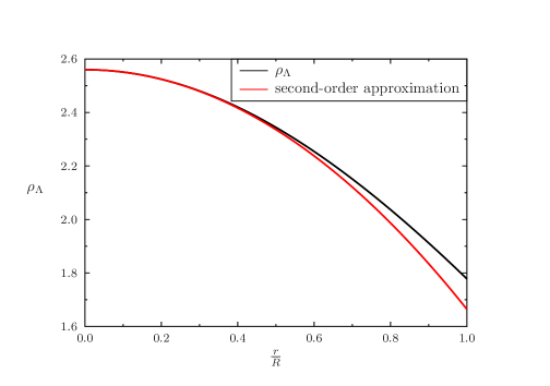
Figure 1: The figure compares the radial dependance of the dark energy density for a star with constant matter density (see eq (15)), radius $R$ = $\frac{32}{7}m\approx 4.6m$ and $\varepsilon_{0}=576\pi r_{0}^{2}$ with its second-order approximation.

In conclusion, the dark energy density $\varepsilon_{\Lambda}$ is not only proportional to the constant mass density with a constant factor, but there is an additional $r$-dependence, which can be approximated for $R$ not too small by a factor of the type $\left(1-\beta r^{2}\right)$. The constant $\beta$ depends in (15) on the constant energy density and on the radius of the star. Assuming that the same relation of the coupling is valid for a matter density which also does depend on $r$, the coupling according to (15) should acquire an even more complicated $r$-dependence. However, in order to keep the matter simple, the ansatz which depends on $r^{2}$, should suffice for a start.

To resume, the considerations in this section suggests the following ansatz for the coupling of the dark energy to the matter density:

$$\varepsilon_{\Lambda} = \alpha\varepsilon_{m}\left[1-\left(\frac{r}{r_{0}}\right)^{2}\right]~{}~{}~{},$$ (16)

where $\alpha$ is a factor as used in [16] and $r_{0}$ is an additional parameter, not to be confused with the parameter used in the model of a constant mass density.

2.2 A non-constant mass distribution

Let us assume that the mass density varies as

$$\varepsilon_{m} = \varepsilon_{0}\left[1-b_{1}\left[\frac{r}{R}\right]^{2}\right]~{}~{}~{},$$ (17)

which simulates realistic calculations [16]. As a length element squared we use

$$ds^{2} = e^{\nu}dt^{2}-e^{\lambda}dr^{2}-r^{2}\left(d\vartheta^{2}+{\rm sin}^{2}\vartheta d\varphi^{2}\right)~{}~{}~{},$$ (18)

where the metric for the interior of the star is proposed to behave as

$$e^{\nu} = \left(1-\frac{r_{s}}{R}\right)e^{\frac{r_{s}}{2\left(R^{3}-r_{s}R^{2}\right)\left(r^{2}-r_{0}^{2}\right)}}$$

$$e^{-\lambda} = 1-\frac{8\pi}{3}\varrho_{0}r^{2}\left(1-b_{1}\frac{3r^{2}}{5R^{2}}\right)~{}~{}~{}.$$ (19)

In order that this connects smoothly to the Schwarzschild metric outside the star, the following condition has to be fulfilled:

$$\frac{8\pi}{3}\varrho_{0}\left(1-\frac{3}{5}b_{1}\right) = \frac{2m}{R^{3}}$$ (20)

Following the same steps as described further above, we arrive for the dark energy density at

$$\varepsilon_{\Lambda}=-\frac{m}{288\pi R^{3}}\frac{1-\frac{3}{5}b_{1}}{\left(1-\frac{2m}{R}\right)^{2}}\varepsilon_{0}\left[1-\frac{2mr^{2}}{\left(1-\frac{3}{5}b_{1}\right)R^{3}}\left(1-\frac{3}{5}b_{1}\frac{r^{2}}{R^{2}}\right)\right]~{}~{}~{}.$$ (21)

The obtained $r$-dependence of the dark energy density on the matter density is now, as expected, more complicated. Nevertheless, the main $(1-br^{2})$-dependence is reproduced, with the correction factor proportional to $b_{1}\frac{r^{2}}{R^{2}}$. Only near the surface ($r$ approximately $R$), this correction is large and may be attributed to the ansatz of the matter density, i.e., it is expected to be not very good there

Again, we arrive at the structure similar to the ansatz (16). Thus, in the next section we use this ansatz to investigate if stars with larger masses than those obtained in [16].

3 Large mass stars

The theory of neutron stars within the pseudo-complex General Relativity is published in [16], assuming a purely linear coupling between the dark energy density $\varepsilon_{\Lambda}$ and the corresponding quantity for the baryonic counterpart $\varepsilon_{m}$:

$$\varepsilon_{\Lambda}=\alpha\varepsilon_{m}$$ (22)

The coupling parameter was chosen to lie in the range $(-1,0)$ and under such conditions, stable solutions were obtained having masses for the baryonic component of up to $[6-7]M_{\odot}$. In the present work, we repeat such calculations using instead of (22) the new coupling relation (16).

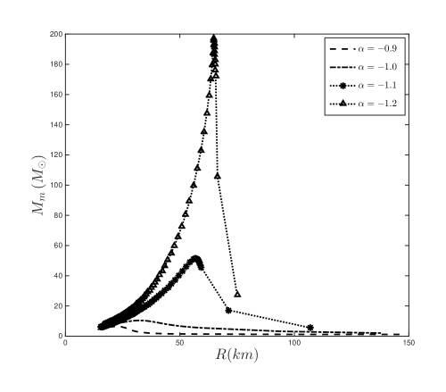
Figure 2: Mass of the baryonic component vs. radius for different values of the coefficient $\alpha$. The central $\Lambda$-term pressure $p_{\Lambda c}$ has been fixed to $P_{\varepsilon_{mc}=10^{-2}\varepsilon_{0}}$, the $r_{0}$ parameter to $100\;km$ and the central baryonic energy density $\varepsilon_{mc}$ between $[4\cdot 10^{-2}-10]\varepsilon_{0}$.

As can be appreciated from Fig. 2, the new coupling relation allows the study of solutions with values of $\alpha<-1$ whose masses can acquire considerable high values of up to 200 solar masses, in comparison with the previous work. This can be understood as a consequence of the stronger fall-off of the new relation toward the radius of the star that causes the dark energy repulsion near the surface to be weaker than the pure linear model (22), while it remains strong near the center. Thus, larger stellar masses can be maintained without collapsing and the repulsion is not strong enough to evaporate the surface.

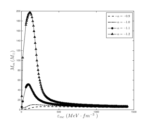
Figure 3: Mass of the baryonic component vs. its central energy density for different values of the coefficient $\alpha$. The central $\Lambda$-term pressure $p_{\Lambda c}$ has been fixed to $P_{\varepsilon_{mc}=10^{-2}\varepsilon_{0}}$, the $r_{0}$ parameter to $100\;km$ and the central baryonic energy density $\varepsilon_{mc}$ between $[4\cdot 10^{-2}-10]\varepsilon_{0}$. Stability can be proven, as explained in [16], investigating how the curve bends for large central density. However, we could not proceed because data on the baryonic properties were not available for that region.

The presence of these more massive solutions can be appreciated in Fig. 3 where already one can identify those which have $\frac{dM}{d\varepsilon_{c}}<0$ and therefore are unstable against small perturbations. Unfortunately, the stability of the solutions with $\frac{dM}{d\varepsilon_{c}}>0$ cannot be completely assured by simple criteria as those employed in [16] and a full perturbative method needs to be carried out. Numerical instabilities inhibited a more profound study. Checking the previous, necessary condition however tells us that at least such massive objects could in principle exist.

Figure 4: Mass of the baryonic component vs. radius for different values of the parameter $r_{0}$. The central $\Lambda$-term pressure $p_{\Lambda c}$ has been fixed to $P_{\varepsilon_{mc}=10^{-2}\varepsilon_{0}}$, the coupling parameter $\alpha$ to $-1.2$ and the central baryonic energy density $\varepsilon_{mc}$ between $[4\cdot 10^{-2}-10]\varepsilon_{0}$.

Within the current study, an additional parameter $r_{0}$ is introduced. As can be seen in Figs. 4 and 5, larger values of $r_{0}$ translate into larger values of the mass corresponding to the baryonic component. The value of $r_{0}$ cannot be a priori determined and therefore four values covering the whole range in which the radii of the solutions lie have been chosen.

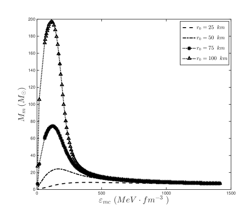
Figure 5: Mass of the baryonic component vs. its central energy density for different values of the parameter $r_{0}$. The central $\Lambda$-term pressure $p_{\Lambda c}$ has been fixed to $P_{\varepsilon_{mc}=10^{-2}\varepsilon_{0}}$, the coupling parameter $\alpha$ to $-1.2$ and the central baryonic energy density $\varepsilon_{mc}$ between $[4\cdot 10^{-2}-10]\varepsilon_{0}$.

4 Conclusions

Using semi-classical Quantum Mechanics, the mass-induced vacuum fluctuations outside and inside a mass distribution were determined within a monopole approximation. Outside a mass distribution the dominant part of the dark energy density falls off as $\frac{1}{r^{6}}$, which is in qualitative agreement to calculations in four dimensions [6]. This finding justifies the ansatz for the dark energy density, as used in the pc-GR [4, 5].

Inside the mass distribution similar calculations lead to a deviation of the linear coupling, as assumed in [16]. The encountered dependence of the coupling between the dark energy density and the mass density includes an extra factor, depending on the radial distance $r$. This finding permits a new, phenomenological ansatz for the coupling, which allows a large dark energy density in the center of a star, therefore sustaining a large mass, and a low density near the surface, thus not evaporating the outer layers of the star, as found in [16].

The discussion presented is a prove of principle that arbitrary large masses of stars are possible, which indicates that the so called black holes may be in fact large stars, though due to the strong gravitational field the physics at the surface and in its interior is expected to change significantly, compared to known neutron stars.

5 Acknowledgement

Peter O. Hess acknowledges the financial support from DGAPA-PAPIIT (IN100315). Isaac Rodríguez acknowledges the financial support from the Alexander von Humboldt Stiftung and FIAS. Gunther Caspar acknowledges financial support from FIAS.

References

- [1] C. W. Misner, K. S. Thorne, J. A. Wheeler, GRAVITATION, (W. H. Freeman and Company, San Francisco, 1973).
- [2] C. M. Will, Living Rev. Relativ. 9 (2006), 3.
- [3] R. A. Hulse and J. H. Taylor, Ap. J. 195 (1975), L51.
- [4] Peter O. Hess und Walter Greiner, Int. J. Mod. Phys. E18 (2009), 51.
- [5] G. Caspar. T. Schönenbach, P. O. Hess, M. Schäfer and W. Greiner, Int. J. Mod. Phys. E 21 (2012), 1250015.
- [6] M. Visser, Phys. Rev. D 54 (1996), 5116.
- [7] T. Schönenbach, G. Caspar, P. O. Hess, T. Boller, A. Müller, M. Schäfer and W. Greiner, MNRAS 430 (2013), 2999.
- [8] T. M. Belloni, A. Sanna, and M. Mendz, MNRAS, 426 (2012), 1701.
- [9] R. I. Hynes, D. Steeghs, J. Casares, P. A. Charles, and K. O’Brian, ApJ, 609 (2004), 317.
- [10] R. C. Reis, A. C. Fabian, R. R. Ross, G. Miniutti, J. M. Miller and C. Reynolds, MNRAS 387 (2008), 1489.
- [11] J. Steiner, J. McClintock, and G. Jeffrey et al., 38th COSPAR Scientific Assembly, 18-15 July, Bremen, Germany, (2010).
- [12] T. Boller and A. Müller, Nuclear Physics: Present and Future, Boppard Proceedings, FIAS Lecture Notes, edt. W. Greiner, (Springer, Heidelberg, 2015), p. 245.
- [13] D. Lai, W. Fu, D. Tsang, J. Horak and C. Ya, Proceedings of the International Astronomical Union, 290 (2012), 57.
- [14] T. Schönenbach, G. Caspar, P. O. Hess, T. Boller, A. Müller, M. Schäfer and W. Greiner, MNRAS 442 (2014), 121.
- [15] D. N. Page und K. S. Thorne, The Astrophys. Jour. 191 (1974), 499.
- [16] I. Rodríguez, P. O. Hess, S. Schramm and W. Greiner, J. Phys. G 41 (2014), 105201.
- [17] N. D. Birrell and P. C. W. Davies. Quantum Fields in Curved Space, (Cambridge University Press, The Edinbugh Building, Cambridge, 1994).
- [18] D. N. Page, Phys. Rev. D 25 (1982), 1499.
- [19] T. Padmanabhan, Phys. Rep. 406 (2005), 49.
- [20] R. Adler, M. Bazin, and M. Schiffer, Introduction to General Relativity, (McGraw-Hill, N.Y., 1975).
- [21] V. Dexheimer and S. Schramm, 2008 Astrophys. J. 683 (2008), 943.
- [22] J. M. Bardeen, K. S. Thorne and D. W. Meltzer, Astrophys. J. 145 (1966), 505.
- [23] K. S. Thorne, Proc. Int. School of Physics ‘Enrico Fermi’ ed L Gratton (New York: Academic) (1966), 166.