Recovering a tree from the lengths of subtrees spanned by a randomly chosen sequence of leaves

Abstract.

Given an edge-weighted tree $\mathbf{T}$ with $n$ leaves, sample the leaves uniformly at random without replacement and let $W_{k}$, $2\leq k\leq n$, be the length of the subtree spanned by the first $k$ leaves. We consider the question, “Can $\mathbf{T}$ be identified (up to isomorphism) by the joint probability distribution of the random vector $(W_{2},\ldots,W_{n})$?” We show that if $\mathbf{T}$ is known a priori to belong to one of various families of edge-weighted trees, then the answer is, “Yes.” These families include the edge-weighted trees with edge-weights in general position, the ultrametric edge-weighted trees, and certain families with equal weights on all edges such as $(k+1)$-valent and rooted $k$-ary trees for $k\geq 2$ and caterpillars.

1. Introduction

1.1. Background and motivation

What features of an edge-weighted tree identify it uniquely up to isomorphism, perhaps within some class of such trees? Here an edge-weighted tree is a connected, acyclic finite graph $\mathbf{T}$ with vertex set $\mathbf{V}(\mathbf{T})$ and edge set $\mathbf{E}(\mathbf{T})$ which is equipped with a function $\mathbf{W}_{\mathbf{T}}:\mathbf{E}(\mathbf{T})\to\mathbb{R}_{++}:=(0,\infty)$. The value of $\mathbf{W}_{\mathbf{T}}(e)$ for an edge $e\in\mathbf{E}(\mathbf{T})$ is called the weight or the length of $e$. Two such trees $\mathbf{T}^{\prime}$ and $\mathbf{T}^{\prime\prime}$ are isomorphic if there is a bijection $\sigma:\mathbf{V}(\mathbf{T}^{\prime})\to\mathbf{V}(\mathbf{T}^{\prime\prime})$ such that:

• $\{u,v\}\in\mathbf{E}(\mathbf{T}^{\prime})$ if and only if $\{\sigma(u),\sigma(v)\}\in\mathbf{E}(\mathbf{T}^{\prime\prime})$,

• $\mathbf{W}_{\mathbf{T}^{\prime}}(\{u,v\})=\mathbf{W}_{\mathbf{T}^{\prime\prime}}(\{\sigma(u),\sigma(v)\})$ for all $\{u,v\}\in\mathbf{E}(\mathbf{T}^{\prime})$.

The question above is, more formally, one of asking for a given class of edge-weighted trees $\mathbb{T}$ about the possible sets $\mathbb{U}$ and functions $\Phi:\mathbb{T}\to\mathbb{U}$ such that for all $\mathbf{T}^{\prime},\mathbf{T}^{\prime\prime}\in\mathbb{T}$ we have $\Phi(\mathbf{T}^{\prime})=\Phi(\mathbf{T}^{\prime\prime})$ if and only if $\mathbf{T}^{\prime}$ and $\mathbf{T}^{\prime\prime}$ are isomorphic. If the class $\mathbb{T}$ consists of edge-weighted trees for which all edges have length $1$ (we will call such objects combinatorial trees for the sake of emphasis), then determining whether two trees in $\mathbb{T}$ are isomorphic is just a particular case of the standard graph isomorphism problem. The general graph isomorphism problem has been the subject of a large amount of work in combinatorics and computer science – [RC77] already speaks of the “graph isomorphism disease” – and, in particular, there are many results on reconstructing the isomorphism type of a graph from the isomorphism types of subgraphs of various sorts (see, for example, the review [Bon91]). There is also a substantial volume of somewhat parallel research on graph isomorphism in computational chemistry (see, for example, [Diu13] for a review). There seems to be considerably less work on determining isomorphism (in the obvious sense) of edge-weighted graphs; of course, in order for two edge-weighted graphs to be isomorphic the underlying combinatorial graphs must be isomorphic, but this does not imply that the best way for checking that two edge-weighted graphs are isomorphic proceeds by first determining whether the underlying combinatorial graphs are isomorphic and then somehow testing whether some isomorphism of the combinatorial graphs is still an isomorphism when the edge-weights are considered.

We begin with a discussion of previous results that address various aspects of the problem of determining when two edge-weighted or combinatorial trees are isomorphic.

A result in [Bed74] gives the following criterion for a bijection $\sigma:\mathbf{V}(\mathbf{T}^{\prime})\to\mathbf{V}(\mathbf{T}^{\prime\prime})$, where $\mathbf{T}^{\prime}$ and $\mathbf{T}^{\prime\prime}$ are combinatorial trees, to be an isomorphism:
if $v_{0},v_{1},\ldots,v_{m}$ is any sequence from $\mathbf{V}(\mathbf{T}^{\prime})\sqcup\mathbf{V}(\mathbf{T}^{\prime\prime})$ such that $v_{0}=v_{m}$ and

$$\{v_{i},v_{j}\}\in\mathbf{E}(\mathbf{T}^{\prime})\sqcup\mathbf{E}(\mathbf{T}^{\prime\prime})\sqcup\{\{u,\sigma(u)\}:u\in\mathbf{V}(\mathbf{T}^{\prime})\}\Longleftrightarrow i-j\equiv\pm 1\mod m,$$

then $m=4$.

The above result is elegant, but, of course, one does not need to apply it to all possible bijections to determine whether two combinatorial trees are isomorphic: there is a much more explicit and efficient procedure, which we now describe for the sake of completeness. First of all, suppose that $\mathbf{T}^{\prime}$ and $\mathbf{T}^{\prime\prime}$ have distinguished vertices $\rho^{\prime}$ and $\rho^{\prime\prime}$ and, in addition to the requirements in the above definition of an isomorphism $\sigma$, we require that $\sigma$ maps $\rho^{\prime}$ to $\rho^{\prime\prime}$; that is, we have rooted trees and we require that an isomorphism maps the root of one tree to the root of the other. The presence of a root allows us to think of a combinatorial tree as a directed graph, where the head of an edge is the vertex that is closer to the root and the tail is the vertex farther from the root. The children of a vertex are the adjacent vertices that are farther from the root and, more generally, the descendants of a vertex $u$ are those vertices $v$ such that the path from the root to $v$ passes through $u$. The subtree spanned by a vertex $u$ and its descendants contains no other vertices and can be thought of as a combinatorial tree rooted at $u$, and we call this subtree the subtree below $u$. Then, two rooted, combinatorial trees $\mathbf{T}^{\prime}$ and $\mathbf{T}^{\prime\prime}$ are isomorphic if the two roots have the same number of children, say $m$, and there is an ordering of these children for each tree such that the subtree below the $i^{\mathrm{th}}$ child of the root of $\mathbf{T}^{\prime}$ is isomorphic (as a rooted, combinatorial tree) to the subtree below the $i^{\mathrm{th}}$ child of the root of $\mathbf{T}^{\prime\prime}$. This observation can be turned into an efficient algorithm (see, for example, [AHU75, Example 3.2]). Now, two combinatorial trees are isomorphic if there is some choice of roots such the resulting rooted, combinatorial trees are isomorphic. A center of a combinatorial tree is a vertex $c$ such that

$$\max_{v\in\mathbf{V}(\mathbf{T})}r_{\mathbf{T}}(c,v)=\min_{u\in\mathbf{V}(\mathbf{T})}\max_{v\in\mathbf{V}(\mathbf{T})}r_{\mathbf{T}}(u,v),$$

where $r_{\mathbf{T}}(u,v)$ is the number of edges in he unique path between $u$ and $v$ for $u,v\in\mathbf{V}(\mathbf{T})$, and a combinatorial tree has either a unique center or two centers that are adjacent. It is therefore possible to determine if two combinatorial trees are isomorphic by rooting each of them at their various centers and checking if any two such rooted, combinatorial trees are isomorphic.

We, however, are interested in whether there are “statistics” of a more numerical character that can be used to decide tree isomorphism. For combinatorial trees, one somewhat obvious possibility is the multiset of eigenvalues of some matrix associated with the tree such as the adjacency matrix or the distance matrix. Unfortunately, the results of [Sch73, BM93, SF83, FGM97, ME11, BES12] show that not only is the isomorphism type of a tree not uniquely determined by the spectrum of its adjacency matrix but for various ensembles of combinatorial trees if one picks a tree uniformly at random from those in the ensemble with $n$ vertices, then the probability there is another tree in the ensemble with an adjacency matrix that has the same spectrum converges to one as $n\to\infty$. The results of [ME11] can be used to show that an analogous phenomenon is present when one considers the spectrum of the matrix of leaf-to-leaf distances.

Two trees have adjacency matrices with the same spectrum if and only if the characteristic polynomials of the adjacency matrices are equal. Given some irreducible representation of the symmetric group on the number of letters equal to the dimension of a square matrix, the immanantal polynomial of the matrix is constructed in the same manner as the characteristic polynomial except that the determinant is replaced by a similarly defined object for which the sign character is replaced by the character of the representation. One might hope that the immanantal polynomials are more successful at deciding isomorphism of combinatorial trees, but a result of [BM93] shows that if the adjacency matrices of two combinatorial trees have the same characteristic polynomials, then they have the same immanantal polynomials for every irreducible representation. We note that [Tur68] already contains an example of two combinatorial trees with adjacency matrices that are explicitly shown to have the same immanantal polynomial.

The greedoid Tutte polynomial of a combinatorial tree $\mathbf{T}$ encodes for each $i$ and $\ell$ the number of subtrees of $\mathbf{T}$ that have $i$ internal vertices and $\ell$ leaves. It was conjectured in [GMOY95] that this information identifies the isomorphism type of a combinatorial tree. However, it was shown in [EG06] that there are infinitely many pairs of nonisomorphic caterpillars that share the same greedoid Tutte polynomial: a caterpillar is a combinatorial tree that consists of some number of internal vertices along a single path and leaves that are each adjacent to one of the internal vertices. This contrasts with the situation for rooted, combinatorial trees; it is shown in [GM89] that there is a two-variable polynomial defined for all rooted, directed graphs (and hence, in particular, for rooted, combinatorial trees) such that two rooted, combinatorial trees have the same polynomial if and only if they are isomorphic. The polynomial in [GM89] is defined recursively, but it is not hard to see that it encodes in a compact manner the total number of vertices in the tree, the number of children of the root, the number of vertices in each of the subtrees below the children of the root, and so on.

The chromatic symmetric function of a graph was introduced in [Sta95]. A proper coloring of a finite graph is a function $\kappa$ from the vertices of the graph to $\mathbb{N}$ such that adjacent vertices are assigned different values. We can introduce an equivalence relation on the proper colorings by declaring that two colorings $\kappa^{\prime}$ and $\kappa^{\prime\prime}$ are equivalent if there is a bijection $\pi:\mathbb{N}\to\mathbb{N}$ such that $\kappa^{\prime\prime}=\pi\circ\kappa^{\prime}$. For a graph with $m$ vertices, each equivalence class gives rise to a partition $\lambda_{1}\geq\lambda_{2}\geq\ldots\geq\lambda_{k}>0$ of $m$ by taking, for any $\kappa$ in the equivalence class, $\lambda_{i}$ to be the $i^{\mathrm{th}}$ largest of the cardinalities $\#\{v:\kappa(v)=j\}$ as $j$ ranges over $\mathbb{N}$. The chromatic symmetric function encodes for each partition of $m$ the number of equivalence classes of colorings that give rise to that partition. It was conjectured in [Sta95] that nonisomorphic combinatorial trees have distinct chromatic symmetric functions. It was shown in [MMW08] that this conjecture is true for caterpillars and that paper also reports on computational results verifying that the conjecture holds for the class of trees with at most $23$ vertices. Further work related to the conjecture for the special case of trees with a single centroid is contained in [OS14].

Our point of departure in this paper is the well-known fact [Zar65, SP69, Bun71, Bun74] that an edge-weighted tree can be reconstructed from its matrix of leaf-to-leaf distances (see [Fel04] for an indication of the importance of this observation in the statistical reconstruction of phylogenetic trees). In fact, an edge-weighted tree with $n$ leaves can be reconstructed from the collection of total lengths of subtrees spanned by all subsets of $m$ leaves provided $n\geq 2m-1$ [PS04]. We remark that the total length of the subtree spanned by a set of leaves is an important quantity in phylogenetics where it is called the phylogenetic diversity of the corresponding set of taxa [HS07].

Given these results, one might imagine that the multiset of leaf-to-leaf distances suffices to identify the isomorphism type of an edge-weighted tree. This is certainly not the case. For example, consider the two combinatorial caterpillars $\mathbf{T}^{\prime}$ and $\mathbf{T}^{\prime\prime}$ with $28$ leaves each, where $\mathbf{T}^{\prime}$ has $3$ internal vertices $a^{\prime},b^{\prime},c^{\prime}$ in order along a path that are adjacent respectively to $2,11,12$ leaves, and $\mathbf{T}^{\prime\prime}$ has $3$ internal vertices $a^{\prime\prime},b^{\prime\prime},c^{\prime\prime}$ in order along a path that are adjacent respectively to $3,14,8$ leaves. Taking the $\binom{25}{2}$ pairs of distinct leaves in $\mathbf{T}^{\prime}$, we see that the distance $2$ appears $\binom{2}{2}+\binom{11}{2}+\binom{12}{2}=122$ times, the distance $3$ appears $2\times 11+11\times 12=154$ times, and the distance $4$ appears $2\times 12=24$ times. Similarly, taking the $\binom{25}{2}$ pairs of distinct leaves in $\mathbf{T}^{\prime\prime}$, we see that the distance $2$ appears $\binom{3}{2}+\binom{14}{2}+\binom{8}{2}=3+91+28=122$ times, the distance $3$ appears $3\times 14+14\times 8=154$ times, and the distance $4$ appears $3\times 18=24$ times. Probabilistically, we have just shown that if we pick two leaves uniformly at random without replacement from an edge-weighted tree, then the isomorphism type of the tree is not uniquely identified by the probability distribution of the distance between the two leaves.

Note in this last example that if we looked at the multisets of lengths of subtrees spanned by three leaves, then we would see the length $3$ appearing $\binom{11}{3}+\binom{12}{3}=335$ times for $\mathbf{T}^{\prime}$ and $\binom{3}{3}+\binom{14}{3}+\binom{8}{3}=421$ times for $\mathbf{T}^{\prime\prime}$, and hence the probability distribution of the length of the subtree spanned by three leaves chosen uniformly at random is not the same for the two trees.

In order to proceed further, we need to introduce some more notation. Write $\mathbf{L}(\mathbf{T})$ for the set of leaves of an edge-weighted tree $\mathbf{T}$. Given a subset $K$ of $\mathbf{L}(\mathbf{T})$, let $\mathbf{W}_{\mathbf{T}}(K)$ be the length of the subtree spanned by $K$; that is, $\mathbf{W}_{\mathbf{T}}(K)$ is the sum of the lengths of the edges in the smallest connected subgraph of $\mathbf{T}$ with a vertex set that contains $K$.

It is possible to calculate the total length of $\mathbf{T}$, that is, $\mathbf{W}_{\mathbf{T}}(\mathbf{L}(\mathbf{T}))$, using the following result from [SS04] that extends one for the special case of $3$-valent trees in [Pau00]. Write $d_{\mathbf{T}}(v)$ for the degree of an interior vertex $v$ of $\mathbf{T}$ (that is, $v\in\mathbf{V}(\mathbf{T})\setminus\mathbf{L}(\mathbf{T})$). For distinct leaves $x,y\in\mathbf{L}(\mathbf{T})$ denote by $I_{\mathbf{T}}(x,y)$ the set of interior vertices on the unique path in $\mathbf{T}$ between $x$ and $y$ and put

$$h_{\mathbf{T}}(x,y):=\prod_{v\in I_{\mathbf{T}}(x,y)}((d_{\mathbf{T}}(v)-1)!)^{-1}.$$

Let $r_{\mathbf{T}}(x,y)$ be the sum of the lengths of the edges in the path between $x$ and $y$. Then,

$$\mathbf{W}_{\mathbf{T}}(\mathbf{L}(\mathbf{T}))=\sum_{\{x,y\}\subseteq\mathbf{L}(\mathbf{T}),x\neq y}h_{\mathbf{T}}(x,y)r_{\mathbf{T}}(x,y).$$

Of course, a similar formula gives $\mathbf{W}_{\mathbf{T}}(K)$ for any $K\subseteq\mathbf{L}(\mathbf{T})$; the path between a pair of leaves of the subtree is the same as the path between them in $\mathbf{T}$, the length of this path is the same in the subtree as it is in $\mathbf{T}$, but the degree of an interior vertex of the subtree can be less than its degree as an interior vertex of $\mathbf{T}$.

Suppose that $\#\mathbf{L}(\mathbf{T})=n$ and $Y_{1},\ldots,Y_{n}$ is a uniformly distributed random listing of $\mathbf{L}(\mathbf{T})$; that is, $Y_{1},\ldots,Y_{n}$ is the result of sampling the leaves of $\mathbf{T}$ uniformly at random without replacement. Set $W_{k}:=\mathbf{W}_{\mathbf{T}}(\{Y_{1},\ldots,Y_{k}\})$ for $2\leq k\leq n$; that is, the random variable $W_{k}$ is the length of the subtree spanned by the first $k$ of the randomly chosen leaves. We write $\mathcal{W}_{\mathbf{T}}$ for the $(n-1)$-dimensional random vector $(W_{2},\ldots,W_{n})$ and call this random vector the random length sequence of $\mathbf{T}$.

In this paper we address the following question.

Question 1.1.

Can we reconstruct the edge-weighted tree $\mathbf{T}$ up to isomorphism from the joint probability distribution of the random length sequence $\mathcal{W}_{\mathbf{T}}$?

Another way of framing this question is the following. Write $y_{1},\ldots,y_{n}$ for the leaves of $\mathbf{T}$ and let $\mathcal{J}_{\mathbf{T}}$ be the multiset with cardinality $n!$ that results from listing the $(n-1)$-dimensional vectors

$$(\mathbf{W}_{\mathbf{T}}(\{y_{\pi(1)},y_{\pi(2)}\}),\mathbf{W}_{\mathbf{T}}(\{y_{\pi(1)},y_{\pi(2)},y_{\pi(3)}\}),\ldots,\mathbf{W}_{\mathbf{T}}(\{y_{\pi(1)},\ldots,y_{\pi(n)}\}))$$

as $\pi$ ranges of the permutations of $[n]:=\{1,\ldots,n\}$. We stress that $\mathcal{J}_{\mathbf{T}}$ is a multiset; that is, we do not know which increasing sequences of lengths go with which ordered listings of the leaves.

Question 1.2.

Can we reconstruct the edge-weighted tree $\mathbf{T}$ up to isomorphism from the multiset of length sequences $\mathcal{J}_{\mathbf{T}}$?

We end this section with some remarks about the problem of reconstructing trees from various so-called decks, as this subject has some similarities to the questions we consider. In [Ula60], Ulam asked whether it is possible to reconstruct the isomorphism type of a graph with at least $3$ vertices from the isomorphism types of the subgraphs obtained by deleting each of the vertices. This question was resolved in the affirmative for combinatorial trees in [Kel57]. Moreover, later results established that it is not necessary to know the forests obtained by deleting every vertex. For example, it was shown in [HP66] that it suffices to know the subtrees obtained by deleting leaves. This latter result was strengthened in [Man70], where it was found that it is only necessary to know which nonisomorphic forests are obtained and not what the multiplicity of each isomorphism type is, and in [Bon69], where it was shown that it suffices to take only those leaves $p$ that are peripheral in the sense that

$$\max_{v\in\mathbf{V}(\mathbf{T})}r_{\mathbf{T}}(p,v)=\max_{v\in\mathbf{V}(\mathbf{T})}\max_{v\in\mathbf{V}(\mathbf{T})}r_{\mathbf{T}}(u,v).$$

Along the same lines, it was established in [Lau83] that it is enough to take only the nonleaf vertices, provided that there are at least three of them. The line of inquiry in [KS85] is the most similar to ours: an example was presented of two trees for which the respective sets of vertices may be paired up in such a way that for each pair the sizes of the trees in the forests produced by removing each element of the pair from its tree are the same, and a necessary and sufficient condition was given for a tree to be uniquely reconstructible from this sort of data, which the authors of [KS85] call the number deck of the tree.

1.2. Overview of the main results

We will answer Question 1.1 in the affirmative for a few different classes of trees. Some classes will have general edge-weights and some classes will be combinatorial trees. It is clear that in the case of general edge-weights we must restrict to trees that have no vertices with degree $2$ because otherwise we can subdivide any edge into arbitrarily many edges with the same total length and the joint probability distribution of the random length sequence will be unchanged – see Figure 1.1. We call such trees simple. The terms irreducible or homomorphically irreducible are also used in the literature.

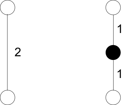
Figure 1.1. Two non-isomorphic edge-weighted trees that cannot be distinguished by the joint probability distribution of their random length sequences.

Our first result is for the the class of stars; that is, edge-weighted trees with $n\geq 3$ leaves that have a single interior vertex. Note that such trees are simple. For any edge-weighted tree with $n$ leaves, $W_{n}$ is a constant (the total length of the tree) and $W_{n}-W_{n-1}$ is a uniformly distributed random pick from the lengths of the $n$ edges that are adjacent to one of the leaves. The following simple result is immediate from this observation.

Theorem 1.3.

For $n\geq 3$ the isomorphism type of a star is uniquely determined by the joint probability distribution of its random length sequence.

The simple trees with two leaves all consist of a single edge and have a random length sequence $(W_{2})$, where $W_{2}$ is the length of that edge, and so the isomorphism type of such a tree is uniquely determined by the joint probability distribution of its random length sequence. The simple trees with three leaves are stars, and it follows from Theorem 1.3 that the isomorphism type of such a tree is uniquely determined by the the joint probability distribution of its random length sequence.

We next consider simple, edge-weighted trees with four leaves.

Theorem 1.4.

For $2\leq n\leq 4$, the isomorphism type of a simple, edge-weighted tree $\mathbf{T}$ with $n$ leaves is uniquely determined by the joint probability distribution of its random length sequence.

The proof of this result is via consideration of possible cases. Similar proofs could be attempted for larger numbers of leaves, but the main reason we include the result is to show how such a proof for even a small number of leaves leads to quite a few cases and because we will need the case of four leaves later.

It is well-known that any simple, combinatorial tree with labeled leaves can be reconstructed from the simple, combinatorial trees spanned by each subset of four leaves (the so-called quartets) [SS03, Theorem 6.3.7]. With this and Theorem 1.4 in mind, one might imagine that the isomorphism type of simple, edge-weighted tree can be determined from the joint probability distribution of $(W_{2},W_{3},W_{4})$. However, putting such a strategy into practice would seem to be rather complicated because there can be two sets of leaves $\{y_{1}^{\prime},y_{2}^{\prime},y_{3}^{\prime},y_{4}^{\prime}\}$ and $\{y_{1}^{\prime\prime},y_{2}^{\prime\prime},y_{3}^{\prime\prime},y_{4}^{\prime\prime}\}$ such that $\{y_{1}^{\prime},y_{2}^{\prime},y_{3}^{\prime},y_{4}^{\prime}\}\neq\{y_{1}^{\prime\prime},y_{2}^{\prime\prime},y_{3}^{\prime\prime},y_{4}^{\prime\prime}\}$ but $\mathbf{W}_{\mathbf{T}}(\{y_{1}^{\prime},y_{2}^{\prime}\})=\mathbf{W}_{\mathbf{T}}(\{y_{1}^{\prime\prime},y_{2}^{\prime\prime}\})$, $\mathbf{W}_{\mathbf{T}}(\{y_{1}^{\prime},y_{2}^{\prime},y_{3}^{\prime}\})=\mathbf{W}_{\mathbf{T}}(\{y_{1}^{\prime\prime},y_{2}^{\prime\prime},y_{3}^{\prime\prime}\})$, and $\mathbf{W}_{\mathbf{T}}(\{y_{1}^{\prime},y_{2}^{\prime},y_{3}^{\prime},y_{4}^{\prime}\})=\mathbf{W}_{\mathbf{T}}(\{y_{1}^{\prime\prime},y_{2}^{\prime\prime},y_{3}^{\prime\prime},y_{4}^{\prime\prime}\})$. One way of ruling out such annoying algebraic coincidences is to assume that the edge-weighted tree $\mathbf{T}$ has edge-weights in general position, by which we mean that the sums of the lengths of any two different (not necessarily disjoint) subsets of edges of $\mathbf{T}$ are not equal.

Theorem 1.5.

The isomorphism type of a simple, edge-weighted tree $\mathbf{T}$ with edge-weights in general position is uniquely determined by the joint probability distribution of its random length sequence.

The last family of edge-weighted trees with general edge-weights whose elements we can identify up to isomorphism from the joint probability distributions of their random length sequences is the class of ultrametric trees. For the sake of completeness, we now define this class. Recall that for leaves $i,j\in\mathbf{L}(\mathbf{T})$ we denote by $r_{\mathbf{T}}(i,j)$ the distance between them; that is, $r_{\mathbf{T}}(i,j)$ is the sum of the lengths of the edges on the unique path between $i$ and $j$. The edge-weighted tree $\mathbf{T}$ is ultrametric if for any leaves $i,j,k\in\mathbf{L}(\mathbf{T})$ we have

$$r_{\mathbf{T}}(i,k)\leq r_{\mathbf{T}}(i,j)\vee r_{\mathbf{T}}(j,k),$$

from which it follows that for any leaves $i,j,k\in\mathbf{L}(\mathbf{T})$ at least two of the distances $r_{\mathbf{T}}(i,j)$, $r_{\mathbf{T}}(i,k)$, and $r_{\mathbf{T}}(j,k)$ are equal while the third is no greater than that common value. Equivalently, an edge-weighted tree $\mathbf{T}$ is ultrametric if, when it is thought of as a real tree (that is, a metric space where the edges are treated as real intervals of varying lengths given by their edge-weights – see, for example, [Eva08]), then there is a (unique) point $\rho$ called the root (which may be in the interior of an edge) such that the distance from $\rho$ to a leaf is the same for all leaves. We will make use of both definitions. It is immediate from the former definition that the subtree of an ultrametric tree spanned of a subset of leaves is itself ultrametric.

Theorem 1.6.

The isomorphism type of an ultrametric, simple, edge-weighted tree $\mathbf{T}$ is uniquely determined by the joint probability distribution of its random length sequence.

Remark 1.7.

The proof of Theorem 1.6 establishes an even stronger result. Namely, the isomorphism type of an ultrametric, simple, edge-weighted tree $\mathbf{T}$ is uniquely determined by the minimal element of $\mathcal{J}_{\mathbf{T}}$ in the lexicographic order.

Remark 1.8.

We call attention to a subtle point in the statements of Theorem 1.5 and Theorem 1.6. Both results say that if we are given the joint probability distribution of the random length sequence of an edge-weighted tree $\mathbf{T}$ – information that certainly includes the number of leaves of $\mathbf{T}$ – and we know, a priori, that $\mathbf{T}$ has a certain extra property (edge-weights in general position or ultrametricity), then we can determine the isomorphism type of $\mathbf{T}$. The theorems do not, however, say whether it is possible to determine from the joint probability distribution of its random length sequence whether a simple, edge-weighted tree $\mathbf{T}$ has its edge-weights in general position or is ultrametric. We do not have results that settle this question, but we say some more about it in 4.1 and believe it is an interesting area for future research.

Observe that if $\mathbf{T}$ is an edge-weighted tree, $a$ is any vertex of $\mathbf{T}$, and $c$ is a constant such that $c\geq\max\{r_{\mathbf{T}}(a,i):i\in\mathbf{L}(\mathbf{T})\}$, then $\tilde{r}_{\mathbf{T}}:\mathbf{L}(\mathbf{T})\times\mathbf{L}(\mathbf{T})\to\mathbb{R}_{+}$ defined by

$$\tilde{r}_{\mathbf{T}}(i,j):=c+\frac{1}{2}(r_{\mathbf{T}}(i,j)-r_{\mathbf{T}}(a,i)-r_{\mathbf{T}}(a,j)),\quad i\neq j,$$

and

$$\tilde{r}_{\mathbf{T}}(i,i):=0,$$

is an ultrametric on $\mathbf{L}(\mathbf{T})$ that arises from suitable edge-weights on $\mathbf{T}$. The metric $\tilde{r}_{\mathbf{T}}$ is often called the Farris transform of $r_{\mathbf{T}}$ – see [DHM07] for a review of the many appearances of this object in various areas from phylogenetics to metric geometry. It might be hoped that an affirmative answer to 1.1 for general edge-weighted trees will follow from Theorem 1.6. However, we have been unable to find an argument which shows that the joint probability distribution of the random length sequence of the tree $\mathbf{T}$ equipped with the new edge-weights is determined by the joint probability distribution of the random length sequence for the original edge-weights.

Suppose that $\mathbf{T}$ is a rooted, simple combinatorial tree with root $\rho$. We can define a partial order on $\mathbf{V}(\mathbf{T})$ by declaring that that $x\leq y$ if $x$ is on the unique path from $\rho$ to $y$. Two vertices $x,y\in\mathbf{V}(\mathbf{T})$ have a unique greatest lower bound in this partial order that we write as $x\wedge y$ and call the most recent common ancestor of $x$ and $y$. The map $\hat{r}_{\mathbf{T}}:\mathbf{L}(\mathbf{T})\times\mathbf{L}(\mathbf{T})\to\mathbb{R}_{+}$ defined by

$$\hat{r}_{\mathbf{T}}(i,j):=\#\{k\in\mathbf{L}(\mathbf{T}):i\wedge j<k\}$$

is an ultrametric on $\mathbf{L}(\mathbf{T})$ and hence it arises from a collection of edge-weights $\hat{\mathbf{W}}_{\mathbf{T}}$ on $\mathbf{T}$. A directed edge $(x,y)$ in $\mathbf{T}$ with $x\leq y$ is necessarily of the form $x=i\wedge j=i\wedge k$ and $y=j\wedge k$ for some $i,j,k\in\mathbf{L}(\mathbf{T})$. If $e=\{x,y\}$ is the corresponding undirected edge, then

$$\begin{split}\hat{\mathbf{W}}_{\mathbf{T}}(e)&=\frac{1}{2}(\hat{r}_{\mathbf{T}}(i,j)-\hat{r}_{\mathbf{T}}(j,k))\\ &=\frac{1}{2}(\#\{\ell\in\mathbf{L}(\mathbf{T}):x<\ell\}-\#\{\ell\in\mathbf{L}(\mathbf{T}):y<\ell\}).\\ \end{split}$$

Therefore, if $\mathbf{T}^{\prime}$ is a subtree of $\mathbf{T}$ spanned by some set of leaves $K\subseteq\mathbf{L}(\mathbf{T})$ and $\mathbf{D}(\mathbf{T}^{\prime})$ is the set of directed edges of $\mathbf{T}^{\prime}$, then we have that the length of $\mathbf{T}^{\prime}$ is

$$\begin{split}\hat{\mathbf{W}}_{\mathbf{T}}(K)&=\frac{1}{2}\sum_{(x,y)\in\mathbf{D}(\mathbf{T}^{\prime})}\left(\sum_{\ell\in\mathbf{L}(\mathbf{T})}\mathbbold{1}\{x<\ell\}-\mathbbold{1}\{y<\ell\}\right)\\ &=\frac{1}{2}\#\{((x,y),\ell)\in\mathbf{D}(\mathbf{T}^{\prime})\times\mathbf{L}(\mathbf{T}):x<\ell,\,y\not<\ell\}.\\ \end{split}$$

The following result is immediate from Theorem 1.6 and 1.7.

Corollary 1.9.

The isomorphism type of a simple, combinatorial tree $\mathbf{T}$ is uniquely determined by the minimal element of the set $\mathcal{J}_{\mathbf{T}}$ of length sequences obtained after designating a root for $\mathbf{T}$ and equipping $\mathbf{T}$ with the edge-weights $\hat{\mathbf{W}}_{\mathbf{T}}$.

We now turn our focus to combinatorial trees and drop the assumption of simplicity. That is, all edge-weights are equal to one and there may be vertices with degree two. We answer Question 1.1 in the affirmative for two families of combinatorial trees.

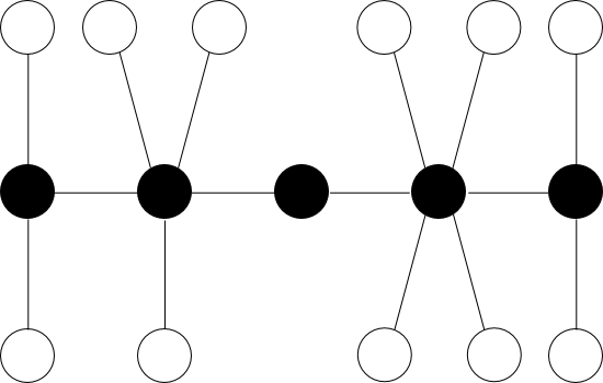
Figure 1.2. A caterpillar tree. Removing the leaves (white vertices) results in a path of length $5$ (black vertices).

First, a combinatorial tree $\mathbf{T}$ is a caterpillar if the deletion of the leaves along with the edges adjacent to them results in a path with $\ell+1$ vertices (and hence $\ell$ edges) – see, for example, Figure 1.2. Choose some direction for the path and number from $0$ to $\ell$ the vertices on the path encountered successively in that direction and write $n_{i}$ for the number of leaves adjacent to the vertex numbered $i$. Note that $n_{0}\geq 1$ and $n_{\ell}\geq 1$. Two sequences $n_{0}^{\prime},\ldots,n_{\ell^{\prime}}^{\prime}$ and $n_{0}^{\prime\prime},\ldots,n_{\ell^{\prime\prime}}^{\prime\prime}$ correspond to isomorphic trees if and only if $\ell^{\prime}=\ell^{\prime\prime}=\ell$, say, and either $n_{i}^{\prime}=n_{i}^{\prime\prime}$, $0\leq i\leq\ell$ or $n_{i}^{\prime}=n_{\ell-i}^{\prime\prime}$, $0\leq i\leq\ell$.

Theorem 1.10.

The isomorphism type of a caterpillar is uniquely determined by the joint probability distribution of its random length sequence. Furthermore, it is possible to determine from the joint probability distribution of the random length sequence of a combinatorial tree whether the tree is a caterpillar.

Our final results are for the classes of (unrooted) $(k+1)$-valent and rooted $k$-ary combinatorial trees. For $k\geq 2$, a $(k+1)$-valent combinatorial tree is a combinatorial tree for which all vertices have degree either $k+1$ (the internal vertices) or $1$ (the leaves). For $k\geq 2$, a rooted $k$-ary combinatorial tree is a combinatorial tree for which one internal vertex (the root) has degree $k$ and the remaining internal vertices have degree $k+1$; the leaves, of course, have degree $1$. When $k=2$ we refer to a rooted $2$-ary combinatorial tree as a rooted binary combinatorial tree. Attaching an extra vertex via and edge to the root of a rooted $k$-ary tree produces a $(k+1)$-valent combinatorial tree.

Theorem 1.11.

The isomorphism type of a $(k+1)$-valent combinatorial tree (respectively, a $k$-ary tree) is uniquely determined by the joint probability distribution of its random length sequence.

In fact, our proof of Theorem 1.11 leads us to a stronger conclusion.

Theorem 1.12.

Fix $n>1$. Let $\mathcal{T}$ be a random $(k+1)$-valent combinatorial tree (respectively, a random $k$-ary combinatorial tree) with $n$ leaves. Then, the probability distribution of the isomorphism type of $\mathcal{T}$ is uniquely determined by the joint probability distribution of its random length sequence.

Note that in Theorem 1.12 there are two sources of randomness in the construction of the random length sequence: we first choose a realization of the random $\mathcal{T}$ and then take an independent uniform random listing of the leaves to build the increasing sequence of subtrees and their lengths.

The rest of the paper consists primarily of proofs of the above results in the order we have presented them. In Section 7 we briefly discuss further open questions related to Question 1.1.

2. Trees with up to $n=4$ leaves: Proof of Theorem 1.4

We begin by looking at Question 1.1 for edge-weighted trees with a small number of leaves and give a proof of Theorem 1.4 that answers Question 1.1 in the affirmative for general, simple edge-weighted trees with $n=2,3$ or $4$ leaves.

The case of Theorem 1.4 for simple trees with $n=2$ leaves is trivial, as all such trees have two leaves and one edge, $\mathcal{W}_{\mathbf{T}}=(W_{2})$ in this case, and $W_{2}$ is the length of the edge.

The case of $n=3$ leaves is only slightly more complicated, as all such trees are star-shaped. Thus, determining $\mathbf{T}$ from $\mathcal{W}_{\mathbf{T}}$ consists of determining its three edge weights. These can be inferred easily from $\mathcal{W}_{\mathbf{T}}$ by looking at the distribution of $W_{3}-W_{2}$, which, since $W_{3}$ is constant (equal to the total length of $\mathbf{T}$), is distributed as a uniform random choice from the three edge weights.

Finally, we give a proof of Theorem 1.4 in the case when $n=4$.

Proof.

For $n=4$ leaves, there are two possible simple combinatorial trees, and hence two possibilities for the shape of $\mathbf{T}$. The first is the star-shaped tree with four edges and one interior vertex. The second is the $3$-valent tree with two interior vertices and one interior edge. See Figure 2.1.

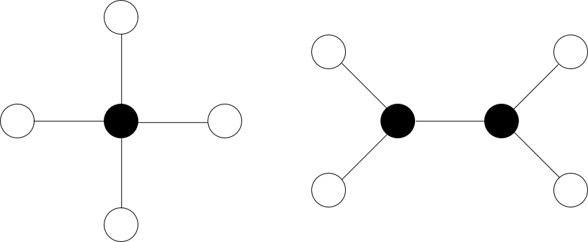
Figure 2.1. The two possible simple combinatorial trees with $n=4$ leaves.

To determine which possibility $\mathbf{T}$ is, we first look at the distribution of $W_{4}-W_{3}$ to find the lengths of the four edges connecting directly to the four leaves. Call these edges pendent. If the sum of the four pendent edge lengths equals $W_{4}$, then $\mathbf{T}$ is star shaped and we have determined $\mathbf{T}$ up to isomorphism. If not, then $\mathbf{T}$ is $3$-valent and the difference between $W_{4}$ and the sum of the pendent edge lengths is the length $e$ of the interior edge. All that is left to determine $\mathbf{T}$ up to isomorphism in this second case is determining how the pendent edges pair on each side of the interior edge.

First, if the multiset of the lengths of pendent edges is of the form $\{a,a,a,a\}$ or $\{a,a,a,b\}$, then $\mathbf{T}$ is already uniquely determined.

Next, if the multiset is of the form $\{a,a,b,b\}$, then we need to distinguish between the case where the leaves with pendent edges of length $a$ are siblings (and thus so are the leaves with pendent edge length $b$) and the case where leaves with pendent edge lengths $a$ and $b$ are paired. In the former case the possible values of $W_{2}$ are $a+a,b+b,a+b+e$ with respective probabilities $\frac{4}{24},\frac{4}{24},\frac{16}{24}$, whereas in the latter case the possible values of $W_{2}$ are $a+b,a+b+e,a+a+e,b+b+e$ with respective probabilities $\frac{8}{24},\frac{8}{24},\frac{4}{24},\frac{4}{24}$, and we can certainly distinguish between the two cases.

If the multiset of pendent edge lengths is of the form $\{a,a,b,c\}$, then there are the following two possibilities:

• the two leaves with pendent edge length $a$ are siblings and the two leaves with pendant edge lengths $b$ and $c$ are siblings, in which case the possible values of $W_{2}$ are $a+a,a+b+e,a+c+c,b+c$ with respective probabilities $\frac{4}{24},\frac{8}{24},\frac{8}{24},\frac{4}{24}$;

• a leaf with pendent edge length $a$ is the sibling of the one with pendent edge length $b$ and the other leaf with pendent edge length $a$ is the sibling of the one with pendent edge length $c$, in which case the possible values of $W_{2}$ are $a+b,a+e,a+a+e,a+b+e,a+c+c,b+c+e$ with respective probabilities $\frac{4}{24},\frac{4}{24},\frac{4}{24},\frac{4}{24},\frac{4}{24},\frac{4}{24}$.

Suppose without loss of generality that $b<c$. If $a<b<c$, then $\mathbb{P}\{W_{2}=a+a\}$ is $\frac{4}{24}$ for (P1) and $0$ for (P2). If $b<a<c$ or $b<c<a$, then $\mathbb{P}\{W_{2}=a+c+e\}$ is $\frac{8}{24}$ for (P1) and $\frac{4}{24}$ for (P2). In all cases we can distinguish between (P1) and (P2).

Finally, if the multiset of pendent edge lengths is of the form $\{a,b,c,d\}$, then there are the following two possibilities:

• the leaf with pendent edge length $a$ is paired with the one with pendent edge length $b$ and the leaf with pendent edge length $c$ is paired with the one with pendent edge length $d$, in which case the possible values of $W_{2}$ are $a+b,c+d,a+c+e,a+d+e,b+c+e,b+d+e$ with common probability $\frac{4}{24}$;

• the leaf with pendent edge length $a$ is paired with the one with pendent edge length $c$ and the leaf with pendent edge length $b$ is paired with the one with pendent edge length $d$, in which case the possible values of $W_{2}$ are $a+c,b+d,a+b+e,a+d+e,b+c+e,c+d+e$ with common probability $\frac{4}{24}$;

• the leaf with pendent edge length $a$ is paired with the one with pendent edge length $d$ and the leaf with pendent edge length $b$ is paired with the one with pendent edge length $c$, in which case the possible values of $W_{2}$ are $a+d,b+c,a+c+e,a+b+e,c+d+e,b+d+e$ with common probability $\frac{4}{24}$;

Suppose without loss of generality that $a<b<c<d$. Then possibility (P3) holds if and only if $\mathbb{P}\{W_{2}=a+b\}>0$ and possibility (P5) holds if and only if $\mathbb{P}\{W_{2}=a+b\}=0$ and $\mathbb{P}\{W_{2}=b+d+e\}>0$, so we can distinguish between (P3), (P4) and (P5). ∎

The argument in the proof of Theorem 1.4 seems rather ad hoc and it does not suggest a systematic approach to obtaining the analogous result for trees with an arbitrary numbers of leaves. The number of simple combinatorial trees with $n$ leaves grows so rapidly with $n$ (see, for example, [Fel04]) that even for trees with a relatively small fixed number of leaves a case-by-case argument seems rather forbidding. Nonetheless, we do conjecture that an affirmative answer to Question 1.1 holds more generally.

3. Trees in general position: Proof of Theorem 1.5

Recall that the edge-weights of a simple, edge-weighted tree $\mathbf{T}$ are in general position if the sum of the lengths of any two distinct subset of edges of $\mathbf{T}$ are not equal.

Proof.

By assumption, if $\{y_{1}^{\prime},\ldots,y_{k}^{\prime}\}$ and $\{y_{1}^{\prime\prime},\ldots,y_{k}^{\prime\prime}\}$ are two subsets of $\mathbf{L}(\mathbf{T})$ such that $\mathbf{W}_{\mathbf{T}}(\{y_{1}^{\prime},\ldots,y_{k}^{\prime}\})=\mathbf{W}_{\mathbf{T}}(\{y_{1}^{\prime\prime},\ldots,y_{k}^{\prime\prime}\})$, then $\{y_{1}^{\prime},\ldots,y_{k}^{\prime}\}=\{y_{1}^{\prime\prime},\ldots,y_{k}^{\prime\prime}\}$. Consequently, if $\{y_{1}^{\prime},\ldots,y_{k}^{\prime}\}$ and $\{y_{1}^{\prime\prime},\ldots,y_{k}^{\prime\prime}\}$ are two subsets of $\mathbf{L}(\mathbf{T})$ such that $\mathbf{W}_{\mathbf{T}}(\{y_{1}^{\prime},\ldots,y_{j}^{\prime}\})=\mathbf{W}_{\mathbf{T}}(\{y_{1}^{\prime\prime},\ldots,y_{j}^{\prime\prime}\})$ for $2\leq j\leq k$, then $\{y_{1}^{\prime},y_{2}^{\prime}\}=\{y_{1}^{\prime\prime},y_{2}^{\prime\prime}\}$ and $y_{j}^{\prime}=y_{j}^{\prime\prime}$ for $3\leq j\leq k$.

Recall that $Y_{1},\ldots,Y_{n}$ are the successive randomly chosen leaves used in the construction of $\mathcal{W}_{\mathbf{T}}=(W_{2},\ldots,W_{n})$.

Because $W_{n}-W_{n-1}$ is the length of the pendent edge attaching $Y_{n}$ to the rest of $\mathbf{T}$, it follows that the set $C:=\{\ell>0:\mathbb{P}\{W_{n}-W_{n-1}=\ell\}>0\}$ has $n$ elements and $\mathbb{P}\{W_{n}-W_{n-1}=\ell\}=\frac{1}{n}$ for each $\ell\in P$. There are at least two leaves of $\mathbf{T}$ that are siblings, and so there exist $\ell^{\prime},\ell^{\prime\prime}\in C$ such that $\mathbb{P}\{W_{2}=\ell^{\prime}+\ell^{\prime\prime}\}>0$. Fix such a pair of lengths and write $x_{1}$ and $x_{2}$ for the (unique) leaves of $\mathbf{T}$ with pendent edges having respective lengths $\ell^{\prime}$ and $\ell^{\prime\prime}$. We have $\mathbb{P}\{W_{2}=\ell^{\prime}+\ell^{\prime\prime}\}=\frac{1}{\binom{n}{2}}$, and the event $\{W_{2}=\ell^{\prime}+\ell^{\prime\prime}\}$ coincides with the event $\{\{Y_{1},Y_{2}\}=\{x_{1},x_{2}\}\}$.

By assumption, the set $D:=\{\ell>0:\mathbb{P}\{W_{3}-W_{2}=\ell\,|\,W_{2}=\ell^{\prime}+\ell^{\prime\prime}\}>0\}$ has $n-2$ elements and $\mathbb{P}\{W_{3}-W_{2}=\ell\,|\,W_{2}=\ell^{\prime}+\ell^{\prime\prime}\}=\frac{1}{n-2}$ for each $\ell\in D$. Index the values of $D$ as $\ell_{3},\ldots,\ell_{n}$ and write $x_{k}$, $3\leq k\leq n$, for the unique leaf of $\mathbf{T}$ that is distance $\ell_{k}$ from the unique vertex of $\mathbf{T}$ that is adjacent to both of the sibling leaves $x_{1}$ and $x_{2}$. We will show that it is possible to determine the leaf-to-leaf distances $r_{\mathbf{T}}(x_{i},x_{j})$, $1\leq i,j\leq n$. As we recalled in the Introduction, this information uniquely identifies the isomorphism type of $\mathbf{T}$.

Again by assumption, the set $E:=\{\ell>0:\mathbb{P}\{W_{4}=\ell\,|\,W_{2}=\ell^{\prime}+\ell^{\prime\prime}\}>0\}$ has $\binom{n-2}{2}$ elements and $\mathbb{P}\{W_{4}=\ell\,|\,W_{2}=\ell^{\prime}+\ell^{\prime\prime}\}=\frac{1}{\binom{n-2}{2}}$ for each $\ell\in E$. For a given $\ell\in E$ there is a unique ordered pair $(x_{i},x_{j})$, $3\leq i\neq j\leq n$, and a unique $e\geq 0$ such that

$$\mathbb{P}\{W_{3}-W_{2}=\ell_{i},\,W_{4}-W_{3}=\ell_{j}-e\,|\,W_{2}=\ell^{\prime}+\ell^{\prime\prime},\,W_{4}=\ell\}>0$$

and

$$\mathbb{P}\{W_{3}-W_{2}=\ell_{j},\,W_{4}-W_{3}=\ell_{i}-e\,|\,W_{2}=\ell^{\prime}+\ell^{\prime\prime},\,W_{4}=\ell\}>0,$$

in which case the two conditional probabilities in question are both $\frac{1}{2}$. Moreover, every ordered pair $(x_{i},x_{j})$, $3\leq i\neq j\leq n$, corresponds to some unique $\ell\in E$ and $e\geq 0$ in this way. The event $\{W_{2}=\ell^{\prime}+\ell^{\prime\prime},\,W_{3}-W_{2}=\ell_{i},W_{4}-W_{3}=\ell_{j}-e,\,W_{4}=\ell\}$ coincides with the event $\{\{Y_{1},Y_{2}\}=\{x_{1},x_{2}\},\,Y_{3}=x_{i},\,Y_{4}=x_{j}\}$ and the event $\{W_{2}=\ell^{\prime}+\ell^{\prime\prime},\,W_{3}-W_{2}=\ell_{j},W_{4}-W_{3}=\ell_{i}-e,\,W_{4}=\ell\}$ coincides with the event $\{\{Y_{1},Y_{2}\}=\{x_{1},x_{2}\},\,Y_{3}=x_{j},\,Y_{4}=x_{i}\}$. Considering the subtree of $\mathbf{T}$ spanned by $\{x_{1},x_{2},x_{3},x_{4}\}$ and ignoring the vertices with degree two to produce a simple tree, the leaves $x_{i}$ and $x_{j}$ are siblings in this simple tree (as are $x_{1}$ and $x_{2}$), and the quantity $e$ is the distance between the vertex in the subtree to which $x_{i}$ and $x_{j}$ are adjacent and the vertex to which $x_{1}$ and $x_{2}$ are adjacent; the lengths of the pendent edges connecting $x_{i}$ and $x_{j}$ to the rest of the subtree are $\ell_{i}-e$ and $\ell_{j}-e$. Thus, if the ordered pair $(x_{i},x_{j})$ corresponds to $\ell\in E$ and $e\geq 0$, then, recalling the notation $r_{\mathbf{T}}$ for the path length distance in $\mathbf{T}$, $r_{\mathbf{T}}(x_{1},x_{2})=\ell^{\prime}+\ell^{\prime\prime}$, $r_{\mathbf{T}}(x_{1},x_{i})=\ell^{\prime}+\ell_{i}$, $r_{\mathbf{T}}(x_{1},x_{j})=\ell^{\prime}+\ell_{j}$, $r_{\mathbf{T}}(x_{2},x_{i})=\ell^{\prime\prime}+\ell_{i}$, $r_{\mathbf{T}}(x_{2},x_{j})=\ell^{\prime\prime}+\ell_{j}$, and $r_{\mathbf{T}}(x_{i},x_{j})=\ell_{i}+\ell_{j}-e$.

Therefore, the joint probability distribution the random length sequence $\mathcal{W}_{\mathbf{T}}$ uniquely determines the matrix of leaf-to-leaf distances in $\mathbf{T}$ and hence the isomorphism type of $\mathbf{T}$.

∎

4. Ultrametric trees: Proof of Theorem 1.6

Recall that $\mathcal{J}_{\mathbf{T}}$ is the set of sequences $(\ell_{2},\ldots,\ell_{n})$ such that $\mathbb{P}\{W_{k}=\ell_{k},\,2\leq k\leq n\}>0$. Write $\prec$ for the usual lexicographic total order on $\mathcal{J}_{\mathbf{T}}$ (that is $\ell^{\prime}\prec\ell^{\prime\prime}$ if in the first coordinate where the two sequences differ the entry of the $\ell^{\prime}$ is smaller than the entry of $\ell^{\prime\prime}$). Equivalently, $\ell^{\prime}\prec\ell^{\prime\prime}$ if either $\ell_{2}^{\prime}<\ell_{2}^{\prime\prime}$ or $\ell_{2}^{\prime}=\ell_{2}^{\prime\prime}$ and for the smallest $k\geq 2$ such that $\ell_{k+1}^{\prime}-\ell_{k}^{\prime}\neq\ell_{k+1}^{\prime\prime}-\ell_{k}^{\prime\prime}$ we have $\ell_{k+1}^{\prime}-\ell_{k}^{\prime}<\ell_{k+1}^{\prime\prime}-\ell_{k}^{\prime\prime}$. In this section we prove Theorem 1.6 by showing that that the tree $\mathbf{T}$ is determined up to isomorphism by the minimal element of $\mathcal{J}_{\mathbf{T}}$.

We use a similar technique (but with a different total order) to establish Theorem 1.11 for $k+1$-valent and rooted $k$-ary combinatorial trees in Section 6.

Proof.

Let $(\ell_{2},\ell_{3},\ldots,\ell_{n})$ be the minimal element of $\mathcal{J}_{\mathbf{T}}$. Write $x_{1},x_{2},\ldots,x_{n}$ for an ordering of $\mathbf{L}(\mathbf{T})$ such that $\ell_{k}=\mathbf{W}_{\mathbf{T}}(\{x_{1},x_{2},\ldots,x_{k}\})$ for $k=2,\ldots,n$.

We will establish by induction that for $2\leq k\leq n$ the ultrametric real tree spanned by the leaves $\{x_{1},x_{2},\ldots,x_{k}\}$ can be reconstructed from $(\ell_{2},\ell_{3},\ldots,\ell_{k})$ and, moreover, if we adopt the convention that we draw ultrametric real trees in the plane with the root at the top and leaves along the bottom, then this particular real tree can be embedded in the plane with the leaves $x_{1},x_{2},\ldots,x_{k}$ in order from left to right.

The claim is certainly true when $k=2$. Suppose the claim is true for $2,3,\ldots,k$.

Write $\mathbf{T}_{k}$ for the ultrametric real tree spanned by $\{x_{1},x_{2},\ldots,x_{k}\}$ and denote the height of $\mathbf{T}_{k}$ by $h_{k}$; that is, $h_{k}$ is the common distance from each of the leaves of $\mathbf{T}_{k}$ to the root $\rho_{k}$ of $\mathbf{T}_{k}$. We can, of course, suppose that $\mathbf{T}_{2}\subset\mathbf{T}_{3}\subset\ldots\subset\mathbf{T}_{n}$.

If $\ell_{k+1}-\ell_{k}\geq h_{k}$, then the ultrametric real tree $\mathbf{T}_{k+1}$ spanned by $\{x_{1},x_{2},\ldots,x_{k},x_{k+1}\}$ must consist of an arc of length

$$h_{k+1}=\frac{1}{2}(\ell_{k+1}-\ell_{k}+h_{k})$$

from the root $\rho_{k+1}$ of $\mathbf{T}_{k+1}$ to the leaf $x_{k+1}$ and an arc of length $\frac{1}{2}(\ell_{k+1}-\ell_{k}-h_{k})$ from “new root” $\rho_{k+1}$ to the “old root” $\rho_{k}$. In this case we can, by the inductive hypothesis, certainly embed $\mathbf{T}_{k+1}$ in the plane with the leaf $x_{k+1}$ to the right of the leaves $x_{1},x_{2},\ldots,x_{k}$.

Assume, therefore, that $\ell_{k+1}-\ell_{k}<h_{k}$. Then the ultrametric real tree $\mathbf{T}_{k+1}$ must consist of $\mathbf{T}_{k}$ and an arc of length $\ell_{k+1}-\ell_{k}$ joining $x_{k+1}$ to a point $y\in\mathbf{T}_{k}$. It will suffice to show that $y$ must be on the arc $[\rho_{k},x_{k}]$ that connects $\rho_{k}$ to $x_{k}$ because there is a unique ultrametric real tree consisting of $\mathbf{T}_{k}$ and an arc of length $\ell_{k+1}-\ell_{k}$ joining a new leaf to a point on the arc $[\rho_{k},x_{k}]$ (this tree must have root $\rho_{k}$ and the point where the arc of length $\ell_{k+1}-\ell_{k}$ attaches to $[\rho_{k},x_{k}]$ must be at distance $h_{k}-(\ell_{k+1}-\ell_{k})$ from $\rho_{k}$) and, moreover, such a tree can be embedded in the plane with the new leaf to the right of the leaves $\{x_{1},x_{2},\ldots,x_{k}\}$.

Suppose, then, that $y$ is not on the arc $[\rho_{k},x_{k}]$. Let $j$ be the maximum of the indices $i<k$ such that $y$ is on the arc connecting $x_{i}$ to $\rho_{k}$. Write $u$ for the point that is closest to $x_{j+1}$ in the subtree spanned by $\{x_{1},x_{2},\ldots,x_{j}\}$ and $\rho_{k}$. Write $v$ for the point that is closest to $x_{j+1}$ in the subtree spanned by $\{x_{1},x_{2},\ldots,x_{j}\}$. Equivalently, $v$ is the point in the subtree spanned by $\{x_{1},x_{2},\ldots,x_{j}\}$ that is closest to $u$. We may, of course, have $u=v$ (which occurs if and only if $h_{j+1}=h_{j}$). By the inductive hypothesis, $u$ and $v$ are on the arc connecting $x_{j}$ to $\rho_{k}$ and

$$r_{\mathbf{T}}(x_{j+1},u)+r_{\mathbf{T}}(u,v)=\ell_{j+1}-\ell_{j}.$$

By construction, $y$ is the point closest to $x_{k+1}$ in the subtree spanned by $\{x_{1},x_{2},\ldots,x_{j}\}$ and $\rho_{k}$. Write $w$ for the point closest to $x_{k+1}$ in the subtree spanned by $\{x_{1},x_{2},\ldots,x_{j}\}$. Equivalently, $w$ is the point in the subtree spanned by $\{x_{1},x_{2},\ldots,x_{j}\}$ that is closest to $y$. We have

$$\mathbf{W}_{\mathbf{T}}(\{x_{1},\ldots,x_{j},x_{k+1}\})-\ell_{j}=r_{\mathbf{T}}(x_{k+1},y)+r_{\mathbf{T}}(y,w).$$

By the definition of $j$, the points $y$ and $u$ are on the arc connecting $x_{j}$ to $\rho_{k}$ and $r_{\mathbf{T}}(u,x_{j})>r_{\mathbf{T}}(y,x_{j})$. This implies that $r_{\mathbf{T}}(u,v)\geq r_{\mathbf{T}}(y,w)$. It also implies, by ultrametricity, that

$$r_{\mathbf{T}}(x_{k+1},y)=r_{\mathbf{T}}(x_{j},y)<r_{\mathbf{T}}(x_{j},u).$$

Consequently,

$$\mathbf{W}_{\mathbf{T}}(\{x_{1},\ldots,x_{j},x_{k+1}\})-\ell_{j}<\ell_{j+1}-\ell_{j}.$$

This, however, contradicts the minimality of $(\ell_{2},\ldots,\ell_{n})$. ∎

Remark 4.1.

As we noted in 1.8, it is interesting to know whether it is possible to determine from the joint probability distribution of the random length sequence whether an edge-weighted tree is ultrametric. The preceding proof of Theorem 1.6 contains a procedure for reconstructing $\mathbf{T}$ from the minimal element of $\mathcal{J}_{\mathbf{T}}$ in the lexicographic order when $\mathbf{T}$ is an ultrametric tree. If $\mathbf{T}$ is an arbitrary edge-weighted tree and this procedure is applied to the minimal element of $\mathcal{J}_{\mathbf{T}}$ in the lexicographic order, then it will still produce an ultrametric tree and so a necessary condition for $\mathbf{T}$ to be ultrametric is that the joint probability distribution of the random length sequence of this ultrametric tree coincides with the joint probability distribution of $\mathcal{W}_{\mathbf{T}}$.

Along the same lines, suppose that $\mathbf{T}$ is an arbitrary edge-weighted tree and, thinking of $\mathbf{T}$ as a real tree, we root it at the unique point $\rho$ such that

$$\max_{v\in\mathbf{L}(\mathbf{T})}r_{\mathbf{T}}(\rho,v)=r^{*}:=\frac{1}{2}\max_{u\in\mathbf{L}(\mathbf{T})}\max_{v\in\mathbf{L}(\mathbf{T})}r_{\mathbf{T}}(u,v).$$

Then $\rho$ will have $k$ children for some $k$. Let $m_{i}$, $1\leq i\leq k$, be the number of leaves $v$ in the subtree below the $i^{\mathrm{th}}$ child of $\rho$ such that $r_{\mathbf{T}}(\rho,v)=r^{*}$. It is clear that $\mathbf{T}$ is ultrametric if and only if $m_{1}+\cdots+m_{k}=n$. Let $n_{1},\ldots,n_{\ell}$ be a listing of the nonzero terms in the list $m_{1},\ldots,m_{k}$. Note for $2\leq j\leq\ell$ that

$$\mathbb{P}\{W_{2}=2r^{*},\ldots,W_{j}=jr^{*}\}=j!\frac{1}{n(n-1)\cdots(n-j+1)}\sum_{1\leq h_{1}<\ldots<h_{j}\leq\ell}n_{h_{1}}\cdots n_{h_{j}}$$

and

$$\max\{j\geq 2:\mathbb{P}\{W_{2}=2r^{*},\ldots,W_{j}=jr^{*}\}>0\}=\ell.$$

Thus, the joint probability distribution of $\mathcal{W}_{\mathbf{T}}$ determines $\ell$ and the values of the elementary symmetric polynomials of degrees $2\leq j\leq\ell$ evaluated at $n_{1},\ldots,n_{\ell}$, and we want to know whether $n_{1}+\cdots+n_{\ell}$, the value of the elementary symmetric polynomial of degree $1$ evaluated at $n_{1},\ldots,n_{\ell}$, is $n$. The elementary symmetric polynomials of degrees $1,2,\ldots,\ell$ in $\ell$ real variables are algebraically independent over the reals, and so we cannot expect to recover $n_{1}+\cdots+n_{\ell}$ from the values of the other elementary symmetric polynomials. However, there are inequalities connecting the values of the various elementary symmetric polynomials that can be used to establish necessary conditions and sufficient conditions for $\mathbf{T}$ to be ultrametric. For example, set

$$p_{1}:=\frac{1}{\ell}(n_{1}+\cdots+n_{\ell})$$

and

$$\begin{split}p_{j}&:=\frac{1}{\binom{\ell}{j}}\sum_{1\leq h_{1}<\ldots<h_{j}\leq\ell}n_{h_{1}}\cdots n_{h_{j}}\\ &=\frac{1}{\binom{\ell}{j}}\frac{n(n-1)\cdots(n-j+1)}{j!}\mathbb{P}\{W_{2}=2r^{*},\ldots,W_{j}=jr^{*}\},\quad 2\leq j\leq\ell.\\ \end{split}$$

If $\alpha_{1},\ldots,\alpha_{\ell}$ and $\beta_{1},\ldots,\beta_{\ell}$ are positive constants such that

$$\alpha_{1}+2\alpha_{2}+\cdots+\ell\alpha_{\ell}=\beta_{1}+2\beta_{2}+\cdots+\ell\beta_{\ell}$$

and

(4.1) $$\alpha_{j}+2\alpha_{j+1}+\cdots+(\ell-j+1)\alpha_{\ell}\geq\beta_{j}+2\beta_{j+1}+\cdots+(\ell-j+1)\beta_{\ell},\quad 2\leq j\leq\ell,$$

then, by [HLP88, Theorem 77, Chapter II]

$$\prod_{j=1}^{\ell}p_{j}^{\alpha_{j}}\leq\prod_{j=1}^{\ell}p_{j}^{\beta_{j}}.$$

Thus, if $\alpha_{2},\ldots,\alpha_{\ell}$ and $\beta_{2},\ldots,\beta_{\ell}$ satisfy the inequalities (4.1) and

$$\gamma:=\sum_{j=2}^{\ell}j(\beta_{j}-\alpha_{j}),$$

then

$$p_{1}\leq\left(\prod_{j=2}^{\ell}p_{j}^{\beta_{j}-\alpha_{j}}\right)^{\frac{1}{\gamma}}$$

when $\gamma>0$, and the opposite inequality hold when $\gamma<0$. This observation leads to necessary conditions and sufficient conditions for $\mathbf{T}$ to be ultrametric.

Remark 4.2.

As we will see in Section 6.4 for $k+1$-valent and rooted $k$-ary combinatorial trees, a somewhat similar proof argument based on the consideration of length sequences that are minimal with respect to a suitable order leads to a stronger result in that case. There we can not only determine $\mathbf{T}$ from the joint probability distribution of its random length sequence, but if we have a random tree $\mathcal{T}$ with a fixed number of leaves, then it is possible to determine the distribution of $\mathcal{T}$ from the joint probability distribution of the random length sequence obtained by first picking a realization of $\mathcal{T}$ and then independently picking a random ordering of the leaves to build a random length sequence.

Formally, we have some space $\mathbb{T}$ of isomorphism types of trees, a corresponding space $\mathbb{S}$ of possible length sequences, and a probability kernel $\mu$ from $\mathbb{T}$ to $\mathbb{S}$, where, for $\mathbf{T}\in\mathbb{T}$, $\nu(\mathbf{T},\cdot)$ is the element of $\mathcal{P}(\mathbb{S})$, the space of probability measures on $\mathbb{S}$, that is the joint probability distribution of the random length sequence built from $\mathbf{T}$. An affirmative answer to 1.1 for a particular $\mathbb{T}$ means that the map $\mathbf{T}\mapsto\nu(\mathbf{T},\cdot)$ from $\mathbb{T}$ to $\mathcal{P}(\mathbb{S})$ is injective. Given an element $\mu$ of $\mathcal{P}(\mathbb{T})$, the space of probability measures on $\mathbb{T}$, let $\mu\nu\in\mathcal{P}(\mathbb{S})$ be defined as usual by $\mu\nu(B)=\int_{\mathbb{T}}\nu(\mathbf{T},B)\,\mu(d\mathbf{T})$ for $B\subseteq\mathcal{S}$. The stronger results obtained in Section 6.4 say that, in the situations considered there, the map $\mu\mapsto\mu\nu$ from $\mathcal{P}(\mathbb{T})$ to $\mathcal{P}(\mathbb{S})$ is injective.

One can ask if an analogous strengthening is also true for ultrametric trees. A proof along the lines of that given for Theorem 1.12 doesn’t appear to apply immediately in this situation where the relevant space $\mathbb{T}$ is uncountable rather than finite. We leave this as one of many open questions.

5. Caterpillar trees: Proof of Theorem 1.10

Recall that a caterpillar is a (not necessarily simple) combinatorial tree such that deleting the leaves of the tree results in a path consisting of $\ell+1$ vertices (and hence $\ell$ edges of length $1$).

Remark 5.1.

Choosing one end of the path, we can label the vertices on path consecutively with $0,1,\ldots,\ell$ and denote by $n_{r}$ the leaves that are attached to vertex $r$ on the path. Both $n_{0}$ and $n_{\ell}$ are non-zero, but the remaining $n_{i}$ may be zero.

The isomorphism types of caterpillars with $n$ leaves are thus seen to be in a bijective correspondence with equivalence classes of nonnegative integer sequences $(n_{0},n_{1},\ldots,n_{\ell-1},n_{\ell})$, where $n=n_{0}+\cdots+n_{\ell}$ and $n_{0},n_{\ell}\neq 0$, and we declare that $(n_{0},n_{1},\ldots,n_{\ell-1},n_{\ell})$ and $(n_{\ell},n_{\ell-1},\ldots,n_{1},n_{0})$ are equivalent.

The proof of the following, which establishes the first claim in Theorem 1.10, is straightforward and we omit it.

Proposition 5.2.

A combinatorial tree $\mathbf{T}$ with $n$ leaves is a caterpillar with an associated path of length $\ell$ if and only if

$$\max\{k:\operatorname{\mathbb{P}}\{W_{2}=k+2\}>0\}=\ell$$

and $W_{n}=\ell+n$ almost surely.

We now turn to the proof of the main claim in Theorem 1.10.

Proof.

Consider a box with $n$ tickets. Each ticket has a label belonging to $\{0,1,\ldots,\ell\}$ and there are $n_{i}$ tickets with label $i$ for $0\leq i\leq\ell$. Let $X_{1},X_{2},\ldots,X_{n}$ be the result of drawing tickets uniformly at random from the box without replacement and noting their labels. Set

$$K_{r}:=\max_{1\leq j\leq r}X_{j}-\min_{1\leq j\leq r}X_{j}.$$

It is clear that $(W_{2},W_{3},\ldots,W_{n})$ has the same joint probability distribution as $(K_{2}+3,K_{3}+3,\ldots,K_{n}+n)$, and so it suffices to show that it is possible to determine $\{(n_{0},n_{1},\ldots,n_{\ell-1},n_{\ell}),(n_{\ell},n_{\ell-1},\ldots,n_{1},n_{0})\}$ from a knowledge of the joint probability distribution of $\mathcal{K}:=(K_{2},\ldots,K_{n})$ (that is, it is possible to determine up to a reflection the vector that gives the number of tickets with each label).

To begin with, note that, as in 5.2,

$$\max\{k:\mathbb{P}\{K_{2}=k\}>0\}=\ell,$$

and so we can determine $\ell$ from the joint probability distribution of $\mathcal{K}$.

Observe next that

$$\begin{split}\mathbb{P}\{K_{2}=\ell\}&=\mathbb{P}\{(X_{1},X_{2})\in\{(0,\ell),(\ell,0)\}\}\\ &=2\frac{n_{0}n_{\ell}}{n(n-1)},\\ \end{split}$$

and

$$\max\{k:\mathbb{P}\{K_{2}=0,\ldots,K_{k}=0,\,K_{k+1}=\ell\}>0\}=n_{0}\vee n_{\ell}.$$

We can thus determine the multiset $\{n_{0},n_{\ell}\}$ and, in particular, $n_{0}+n_{\ell}$.

For $1\leq r<\frac{\ell}{2}$ we have

$$\begin{split}&\mathbb{P}\{K_{2}=r,\,K_{3}=\ell\}\\ &\quad=\mathbb{P}\{(X_{1},X_{2},X_{3})\in\{(0,r,\ell),(r,0,\ell),(\ell,\ell-r,0),(\ell-r,\ell,0)\}\}\\ &\quad=\frac{2n_{0}(n_{r}+n_{\ell-r})n_{\ell}}{n(n-1)(n-2)},\\ \end{split}$$

and so we can determine $n_{r}+n_{\ell-r}$. If $\ell$ is even, then

$$\begin{split}&\mathbb{P}\{K_{2}=\frac{\ell}{2},\,K_{3}=\ell\}\\ &\quad=\mathbb{P}\left\{(X_{1},X_{2},X_{3})\in\left\{\left(0,\frac{\ell}{2},\ell\right),\left(\frac{\ell}{2},0,\ell\right),\left(\ell,\frac{\ell}{2},0\right),\left(\frac{\ell}{2},\ell,0\right)\right\}\right\}\\ &\quad=\frac{4n_{0}n_{\frac{\ell}{2}}n_{\ell}}{n(n-1)(n-2)},\\ \end{split}$$

and so we can determine $n_{\frac{\ell}{2}}$.

Also,

$$\begin{split}\mathbb{P}\{K_{2}=0\}&=\sum_{i=0}^{\ell}\mathbb{P}\{X_{1}=r,X_{2}=r\}\\ &=\frac{\sum_{r=0}^{\ell}n_{r}(n_{r}-1)}{n(n-1)}\\ &=\frac{\sum_{r=0}^{\ell}n_{r}^{2}-n}{n(n-1)}\\ \end{split}$$

and, for $1\leq k\leq\ell$,

$$\begin{split}\mathbb{P}\{K_{2}=k\}&=\sum_{r=0}^{\ell-k}\mathbb{P}\{(X_{1},X_{2})\in\{(r,r+k),(r+k,r)\}\}\\ &=\frac{2\sum_{r=0}^{\ell-k}n_{r}n_{r+k}}{n(n-1)}.\\ \end{split}$$

We can therefore determine $\sum_{r=0}^{\ell-k}n_{r}n_{r+k}$ for $0\leq k\leq\ell$.

We claim that we the information we have just derived suffices to determine $\{(n_{0},n_{1},\ldots,n_{\ell-1},n_{\ell}),(n_{\ell},n_{\ell-1},\ldots,n_{1},n_{0})\}$. That is, if $n_{0}^{\prime},\ldots,n_{\ell}^{\prime}$ is a sequence with

$$n_{0}+\cdots+n_{\ell}=n_{0}^{\prime}+\cdots+n_{\ell}^{\prime}=n,$$

$$n_{r}+n_{\ell-r}=n_{r}^{\prime}+n_{\ell-r}^{\prime}$$

for $0\leq r\leq\ell$, and

$$\sum_{r=0}^{\ell-k}n_{r}n_{r+k}=\sum_{r=0}^{\ell-k}n_{r}^{\prime}n_{r+k}^{\prime}$$

for $0\leq k\leq\ell$, then either $n_{r}=n_{r}^{\prime}$ for $0\leq r\leq\ell$ or $n_{r}=n_{\ell-r}^{\prime}$ for $0\leq r\leq\ell$.

To see that this is so, introduce the Fourier transforms

$$g(z):=\sum_{k=0}^{\ell}n_{k}e^{izk}$$

and

$$g^{\prime}(z):=\sum_{k=0}^{\ell}n_{k}^{\prime}e^{izk}$$

for $z\in\mathbb{C}$. These are entire functions that uniquely determine $n_{0},\ldots,n_{\ell}$ and $n_{0}^{\prime},\ldots,n_{\ell}^{\prime}$. Note that

$$\sum_{k=0}^{\ell}n_{\ell-k}e^{izk}=e^{iz\ell}g(-z),$$

and a similar formula holds for $g^{\prime}$. It will thus suffice to show that either $g(z)=g^{\prime}(z)$ or $g(z)=e^{iz\ell}g^{\prime}(-z)$ (equivalently, $g^{\prime}(z)=e^{iz\ell}g(-z)$).

It follows from the assumption that

$$\sum_{r=0}^{\ell-k}n_{r}n_{r+k}=\sum_{r=0}^{\ell-k}n_{r}^{\prime}n_{r+k}^{\prime}$$

for $0\leq k\leq\ell$ that if we define $N:\mathbb{Z}\to\mathbb{Z}$ by

$$N(j)=\begin{cases}n_{j},&\quad 0\leq j\leq\ell,\\ 0,&\quad\text{otherwise,}\end{cases}$$

and define $N^{\prime}$ similarly, then

$$\sum_{\{r,j\in\mathbb{Z}:r-j=k\}}N(r)N(j)=\sum_{\{r,j\in\mathbb{Z}:r-j=k\}}N^{\prime}(r)N^{\prime}(j)$$

for all $k\in\mathbb{Z}$ and hence

$$g(z)g(-z)=g^{\prime}(z)g^{\prime}(-z)$$

for all $z\in\mathbb{C}$. By Theorem 2.2 in [RS82], there exist finitely supported functions $C:\mathbb{Z}\to\mathbb{Z}$ and $D:\mathbb{Z}\to\mathbb{Z}$ such that if we set

$$\phi(z):=\sum_{k\in\mathbb{Z}}C(k)e^{izk}$$

and

$$\psi(z):=\sum_{k\in\mathbb{Z}}D(k)e^{izk},$$

then

$$g(z)=\phi(z)\psi(z)$$

and

$$g^{\prime}(z)=\phi(z)\psi(-z).$$

It follows from the assumption that

$$n_{r}+n_{\ell-r}=n_{r}^{\prime}+n_{\ell-r}^{\prime}$$

for $0\leq r\leq\ell$ that

$$g(z)+e^{iz\ell}g(-z)=g^{\prime}(z)+e^{iz\ell}g^{\prime}(-z)$$

for all $z\in\mathbb{C}$. Therefore,

$$\phi(z)\psi(z)+e^{iz\ell}\phi(-z)\psi(-z)=\phi(z)\psi(-z)+e^{iz\ell}\phi(-z)\psi(z)$$

and hence

$$(\phi(z)-e^{iz\ell}\phi(-z))(\psi(z)-\psi(-z))=0$$

for all $z\in\mathbb{C}$. Because the functions $z\mapsto\phi(z)-e^{iz\ell}\phi(-z)$ and $z\mapsto\psi(z)-\psi(-z)$ are both entire, we must have either that $\phi(z)=e^{iz\ell}\phi(-z)$ for all $z\in\mathbb{C}$ or $\psi(z)=\psi(-z)$ for all $z\in\mathbb{C}$. If $\phi(z)=e^{iz\ell}\phi(-z)$ for all $z\in\mathbb{C}$, then

$$g^{\prime}(z)=\phi(z)\psi(-z)=e^{iz\ell}\phi(-z)\psi(-z)=e^{iz\ell}g(-z)$$

and $n_{i}=n_{\ell-i}^{\prime}$ for $0\leq i\leq\ell$. If $\psi(z)=\psi(-z)$ for all $z\in\mathbb{C}$, then

$$g^{\prime}(z)=\phi(z)\psi(-z)=\phi(z)\psi(z)=g(z)$$

and $n_{r}=n_{r}^{\prime}$ for $0\leq r\leq\ell$. ∎

6. $k+1$-valent and rooted $k$-ary trees

We now turn our focus to the cases of $(k+1)$-valent and $k$-ary trees. Recall that a $(k+1)$-valent tree is a tree with all vertices of degree either $k+1$ or $1$. For $k\geq 2$ a rooted $k$-ary tree is a tree with one vertex of degree $k$ and the rest of degrees either $k+1$ or $1$. We refer to the rooted $2$-ary tree as a rooted binary tree. Note that any $k$-ary tree is obtained by removing one leaf of a suitable $(k+1)$-valent trees.

Our general proof methodology for these families of trees is similar to that used in Section 4 for ultrametric trees. We first define a particular class of sequences that can appear as elements of $\mathcal{J}_{\mathbf{T}}$ (the down-split sequences) and a total order on such sequences. We then show that the minimal down-split sequence in $\mathcal{J}_{\mathbf{T}}$ uniquely identifies $\mathbf{T}$.

The idea of the proof is the same for all $k$ and depends on the following fact.

Lemma 6.1.

Let $\mathbf{T}$ be a $(k+1)$-valent tree or a rooted $k$-ary tree and let $\SS$ be a subtree of $\mathbf{T}$. Then $\SS$ is a rooted $k$-ary tree if and only if

$$\#\mathbf{E}(\SS)=\frac{k}{k-1}(\#\mathbf{L}(\SS)-1).$$

Proof.

Because $\SS$ is a subtree of $\mathbf{T}$, every interior vertex of $\SS$ has degree at most $k+1$. Write $d_{1}:=\#\mathbf{L}(\SS),d_{2},\ldots,d_{k+1}$ for the number of vertices of $\SS$ of degrees $1,2,\ldots,k+1$. We need to show that $d_{j}=0$ for $1<j\leq k-1$ and $d_{k}=1$, or, equivalently, that $d_{k}=1$ and $d_{k+1}=\sum_{j=2}^{k+1}d_{j}-1=\#\mathbf{V}(\SS)-d_{1}-1=\#\mathbf{E}(\SS)-d_{1}$. This is in turn equivalent to showing that

$$\sum_{j=2}^{k+1}jd_{j}=k+(k+1)(\#\mathbf{E}(\SS)-d_{1}),$$

which, by the “handshaking identity”

$$2\#\mathbf{E}(\SS)=\sum_{j=1}^{k+1}jd_{j},$$

becomes

$$2\#\mathbf{E}(\SS)-d_{1}=k+(k+1)(\#\mathbf{E}(\SS)-d_{1})$$

or, upon rearranging,

$$\#\mathbf{E}(\SS)=\frac{k}{k-1}(d_{1}-1)=\frac{k}{k-1}(\#\mathbf{L}(\SS)-1).$$

∎

For simplicity of notation we present the details of the proof for the case of (unrooted) $3$-valent trees and rooted binary trees (that is, $k=2$). We end in Section 6.4 with a discussion of the extension to general $k$.

6.1. $3$-valent and rooted binary trees

Our proof of Theorem 1.11 begins with an analysis of random length sequences for marked (also known as planted) $3$-valent trees. A marked $3$-valent tree $(\mathbf{T},v)$ is an $3$-valent tree $\mathbf{T}$ and a distinguished leaf $v$ of $\mathbf{T}$. We define the modified random length sequence $\mathcal{W}_{(\mathbf{T},v)}$ of $(\mathbf{T},v)$ to be the random length sequence $\mathcal{W}_{\mathbf{T}}$ of $\mathbf{T}$ conditioned on $Y_{1}=v$.

6.2. Down-split sequences

We need to distinguish some particular sequences that appear in the support of $\mathcal{W}_{(\mathbf{T},v)}$.

Remark 6.2.

As usual, we can define a partial order on $\mathbf{V}(\mathbf{T})$ by declaring that $x$ precedes $y$ if $x\neq y$ is on the path between $v$ and $y$, and we can extend this partial order to a total order $<$ such that if $w,x,y,z$ are such that $w$ and $x$ are not comparable in the partial order but $w<x$, $w$ precedes $y$ in the partial order, and $x$ precedes $z$ in the partial order, then $y<z$. Such a total order corresponds to embedding $\mathbf{T}$ in the plane and listing the elements of $\mathbf{V}(\mathbf{T})$ in the order they are encountered as one walks around $\mathbf{T}$ starting from $v$.

Suppose that $v=y_{1}<y_{2}<\ldots<y_{n}$ is the ordered listing of $\mathbf{L}(\mathbf{T})$. Set $s_{k}=\mathbf{W}_{\mathbf{T}}(\{y_{1},\ldots,y_{k}\})$, $2\leq k\leq n$. If $s_{k}=2k-2$, then the subtree spanned by the $k$ leaves $\{y_{1},\ldots,y_{k}\}$ has $2k-2$ edges and hence, by Lemma 6.1, this subtree is a binary tree. If we write $o$ for the vertex adjacent to the marked leaf $v$, denote by $v^{\prime},v^{\prime\prime}$ the other two vertices adjacent to $o$, and suppose that $v^{\prime}<v^{\prime\prime}$, then it must be the case that $\{y_{2},\ldots,y_{k_{s}}\}=\{y\in\mathbf{L}(\mathbf{T}):v^{\prime}\leq y\}$. Write $\mathbf{T}^{\prime}$ (respectively, $\mathbf{T}^{\prime\prime}$) for the subtree of $\mathbf{T}$ consisting of $w$ and the vertices $u$ such that $v^{\prime}$ (respectively, $v^{\prime\prime}$) is on the path from $o$ to $u$. The sequence $(s_{2}^{\prime},\ldots,s_{n^{\prime}}^{\prime}):=(s_{2}-1,\ldots,s_{k_{s}}-1)$ satisfies $s_{k}^{\prime}=\mathbf{W}_{\mathbf{T}^{\prime}}(o,y_{2},\ldots,y_{k})$ for $2\leq k\leq n^{\prime}=k_{s}$. The sequence $(s_{2}^{\prime\prime},\ldots,s_{n^{\prime\prime}}^{\prime\prime}:=(s_{k_{s}+1}-(2k_{s}-2),\ldots,s_{n}-(2k_{s}-2))$ satisfies $s_{k}^{\prime\prime}=\mathbf{W}_{\mathbf{T}^{\prime\prime}}(o,y_{k_{s}+1},\ldots,y_{k_{s}+k-1})$ for $2\leq k\leq n^{\prime\prime}=n-k_{s}+1$.

Definition 6.3.

A down-split sequence is an element of the class of increasing sequences of positive integers defined recursively as follows. The sequence

$$s=(1)$$

is a down-split sequence.

A sequence $s=(s_{2},\ldots,s_{n})$, $n>2$, is down-split if

$$\{2\leq k<n\colon s_{k}=2k-2\}\neq\emptyset$$

and, setting

$$k_{s}=\inf\{2\leq k<n\colon s_{k}=2k-2\},$$

• $(s_{2}-1,\ldots,s_{k_{s}}-1)$ is down-split,

• $(s_{k_{s}+1}-(2k_{s}-2),\ldots,s_{n}-(2k_{s}-2))$ is down-split.

The index $k_{s}$ is the splitting index of $s$.

Example 6.4.

For $n=3$, the sequence $s=(s_{2},s_{3})=(2,3)$ is a down-split sequence. Here $k_{s}=2$, $(s_{2}-1,\ldots,s_{k_{s}}-1)=(1)$ and $(s_{k_{s}+1}-(2k_{s}-2),\ldots,s_{n}-(2k_{s}-2))=(1)$.

The following result is immediate from 6.2.

Lemma 6.5.

For every marked $3$-valent tree $(\mathbf{T},v)$ there is at least one down-split sequence $s$ with

$$\operatorname{\mathbb{P}}\{\mathcal{W}_{(\mathbf{T},v)}=s\}>0.$$

We record the following fact for later use.

Lemma 6.6.

If $s=(s_{2},\ldots,s_{n})$ is a down-split sequence then $s_{n}=2n-3$.

Proof.

This follows easily by induction. If $s$ splits at $k_{s}$, then, as

$$(s_{2}^{\prime},\ldots,s_{n^{\prime}}^{\prime})=(s_{k_{s}+1}-(2k_{s}-2),\ldots,s_{n}-(2k_{s}-2))$$

is a down-split sequence with $n^{\prime}=n-k_{2}+1$, we have by the inductive hypothesis that

$$s_{n}-(2k_{s}-2)=2(n-k_{s}+1)-3$$

and the claim follows. ∎

Example 6.7.

Given any down-split sequence $s$, it is possible to reverse the argument in 6.2 and construct a marked $3$-valent tree with a suitable total ordering on its vertices such that $s$ is the corresponding down-split sequence. However, a marked $3$-valent tree $(\mathbf{T},v)$ is not uniquely identified by an arbitrary down-split sequence in the support of $\mathcal{W}_{(\mathbf{T},v)}$, as the example in Figure 6.1 shows.

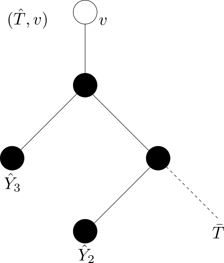
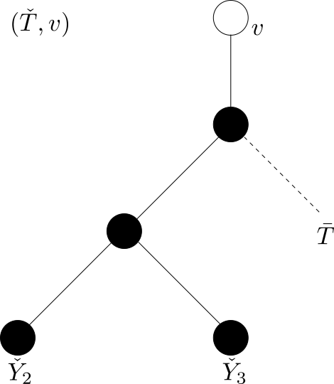
Figure 6.1. Two marked binary trees $(\hat{\mathbf{T}},v)$ and $(\check{\mathbf{T}},v)$ with particular realizations of the random selection of leaves.

Write $(\hat{Y}_{1},\ldots,\hat{Y}_{n})$ and $(\check{Y}_{1},\ldots,\check{Y}_{n})$ for the random selections of the leaves of $\hat{\mathbf{T}}$ and $\check{\mathbf{T}}$. Suppose that the realizations are such that $\hat{Y}_{k}=\check{Y}_{k}\in\bar{\mathbf{T}}$ for $4\leq k\leq n$ and that these leaves of the subtree $\bar{\mathbf{T}}$ appear in an order of the type discussed in 6.2. The corresponding realizations for the modified random length sequences are equal. The common value $(3,4,\ldots)$ is a down-split sequence with splitting index $3$. Thus, two non-isomorphic marked $3$-valent trees can have a common down-split sequence in the supports of their modified random length sequences. Note that the common down-split sequence results from taking the leaves of $\check{\mathbf{T}}$ according to an order of the type described in 6.2, but this is not the case for $\hat{\mathbf{T}}$.

With 6.7 in mind we see that it would be useful to have a way of recognizing down-split sequences in the support of $\mathcal{W}_{(\mathbf{T},v)}$ that result from realizations where the leaves are selected in an order that arises from a suitable total order on the vertices of $\mathbf{T}$. The key is the following total order on down-split sequences. We re-use the notation $\prec$ that was used in Section 4 for the lexicographic order.

Definition 6.8.

Define a total order $\prec$ on the set of down-split sequences of a given length recursively as follows. Firstly, $(1)\prec(1)$ does not hold. Next, let $s,r$ be down-split sequences indexed by $\{2,\ldots,n\}$ with respective splitting indices $k_{s}$ and $k_{r}$. Set

$$s^{\prime}=(s_{2}-1,\ldots,s_{k_{s}}-1),\quad r^{\prime}=(r_{2}-1,\ldots,r_{k_{r}}-1),$$

and

$$s^{\prime\prime}=(s_{k_{s}+1}-(2k_{s}-2),\ldots,s_{n}-(2k_{s}-2)),\quad r^{\prime\prime}=(r_{k_{r}+1}-(2k_{r}-2),\ldots,r_{n}-(2k_{r}-2)).$$

Declare that

$$s\prec r$$

if

$$k_{s}<k_{r}$$

or

$$k_{s}=k_{r}\quad\text{and}\quad s^{\prime}\prec r^{\prime}$$

or

$$k_{s}=k_{r}\quad\text{and}\quad s^{\prime}=r^{\prime}\quad\text{and}\quad s^{\prime\prime}\prec r^{\prime\prime}.$$

The next result follows easily by induction.

Lemma 6.9.

The binary relation $\prec$ is a total order on the set of down-split sequences of a given length.

Definition 6.10.

The minimal down-split sequence for a marked $3$-valent tree $(\mathbf{T},v)$ is the minimal element (with respect to the total order $\prec$) of the set

$$\{s\text{ down-split }\colon\operatorname{\mathbb{P}}\{\mathcal{W}_{(\mathbf{T},v)}=s\}>0\}.$$

We now proceed to establish some results that culminate in showing that $(\mathbf{T},v)$ is determined by its minimal down-split sequence.

Lemma 6.11.

Let $(\mathbf{T},v)$ be a marked $3$-valent tree, with modified random length sequence $\mathcal{W}_{(\mathbf{T},v)}=(W_{2},\ldots,W_{n})$ constructed from the random sequence of leaves $(Y_{1},\ldots,Y_{n})$ with $Y_{1}=v$. Denote by $o$ the vertex adjacent to the marked leaf $v$ and denote by $v^{\prime},v^{\prime\prime}$ the other two vertices adjacent to $o$. Write $\mathbf{T}^{\prime}$ (respectively, $\mathbf{T}^{\prime\prime}$) for the subtree of $\mathbf{T}$ consisting of $o$ and the vertices $u$ such that $v^{\prime}$ (respectively, $v^{\prime\prime}$) is on the path from $o$ to $u$. Set

$$m:=\inf\{k\colon\operatorname{\mathbb{P}}\{W_{k}=2k-2\}>0\}.$$

Then $W_{m}=2m-2$ if and only if

$$Y_{2},\ldots,Y_{m}\in\mathbf{L}(\mathbf{T}^{\prime})\text{ and }Y_{m+1},\ldots,Y_{n}\in\mathbf{L}(\mathbf{T}^{\prime\prime}),$$

or vice versa.

Proof.

If $Y_{2},\ldots,Y_{m}\in\mathbf{L}(\mathbf{T}^{\prime})$ and $Y_{m+1},\ldots,Y_{n}\in\mathbf{L}(\mathbf{T}^{\prime\prime})$, then the subtree spanned by $\{v,Y_{2},\ldots,Y_{m}\}$ consists of the leaf $v$ adjoined to $\mathbf{T}^{\prime}$ via an edge to the vertex $o$. This subtree is a rooted binary tree with root $o$. It follows from Lemma 6.1 that $W_{m}=2m-2$.

For the other direction, assume that $W_{m}=2m-2$. By Lemma 6.1, the subtree $\SS$ spanned by $\{v,Y_{2},\ldots,Y_{m}\}$ is a rooted binary tree with $m$ leaves. We have $\mathbf{L}(\SS)\subseteq\mathbf{L}(\mathbf{T})$, $v\in\mathbf{L}(\SS)$, and $\mathbf{L}(\SS)\setminus\{v\}\subseteq(\mathbf{L}(\mathbf{T}^{\prime})\setminus\{o\})\cup(\mathbf{L}(\mathbf{T}^{\prime\prime})\setminus\{o\})$. We need to show that $\SS$ consists of the leaf $v$ adjoined to either $\mathbf{T}^{\prime}$ or $\mathbf{T}^{\prime\prime}$ via an edge to the vertex $o$ that is common to both $\mathbf{T}^{\prime}$ and $\mathbf{T}^{\prime\prime}$.

By the construction prior to the statement of Lemma 6.5 we know that

$$m\leq\#\mathbf{L}(\mathbf{T}^{\prime})\wedge\#\mathbf{L}(\mathbf{T}^{\prime\prime})$$

and so if $\mathbf{L}(\mathbf{T}^{\prime})\setminus\{o\}\subseteq\mathbf{L}(\SS)\setminus\{v\}$, then $\mathbf{L}(\mathbf{T}^{\prime\prime})\cap\mathbf{L}(\SS)=\mathbf{L}(\mathbf{T}^{\prime\prime})\setminus\{o\}\cap\mathbf{L}(\SS)\setminus\{v\}=\emptyset$ and similarly with the roles of $\mathbf{T}^{\prime}$ and $\mathbf{T}^{\prime\prime}$ reversed.

We can rule out the possibility that $\mathbf{L}(\SS)$ intersects both $\mathbf{L}(\mathbf{T}^{\prime})$ and $\mathbf{L}(\mathbf{T}^{\prime\prime})$ as follows. If $\mathbf{L}(\mathbf{T}^{\prime})\cap\mathbf{L}(\SS)\neq\emptyset$ and $\mathbf{L}(\mathbf{T}^{\prime\prime})\cap\mathbf{L}(\SS)\neq\emptyset$, then $\mathbf{L}(\mathbf{T}^{\prime})\cap\mathbf{L}(\SS)$ must be a proper subset of $\mathbf{L}(\mathbf{T}^{\prime})\setminus\{o\}$ and $\mathbf{L}(\mathbf{T}^{\prime\prime})\cap\mathbf{L}(\SS)$ must be a proper subset of $\mathbf{L}(\mathbf{T}^{\prime\prime})\setminus\{o\}$. If $\mathbf{L}(\mathbf{T}^{\prime})\cap\mathbf{L}(\SS)$ is a proper, nonempty subset of $\mathbf{L}(\mathbf{T}^{\prime})\setminus\{o\}$, then $\SS$ must have a degree $2$ vertex that belongs to $\mathbf{V}(\mathbf{T}^{\prime})\setminus\{o\}$, and similarly for $\mathbf{T}^{\prime\prime}$. However, $\SS$ is a rooted binary tree and cannot have two or more vertices of degree $2$.

Finally, we need to rule out the possibility of $\mathbf{L}(\SS)\setminus\{v\}$ is a proper subset of $\mathbf{L}(\mathbf{T}^{\prime})\setminus\{o\}$ or $\mathbf{L}(\mathbf{T}^{\prime\prime})\setminus\{o\}$. However, if $\mathbf{L}(\SS)\setminus\{v\}$ is a proper subset of $\mathbf{L}(\mathbf{T}^{\prime})\setminus\{o\}$, then $\SS$ would have at least one degree $2$ vertex in that belongs to $\mathbf{V}(\mathbf{T}^{\prime})\setminus\{o\}$ as well as the degree $2$ vertex $o$, which contradicts $s$ being a rooted binary tree. The same argument holds with $\mathbf{T}^{\prime\prime}$ in place of $\mathbf{T}^{\prime}$. ∎

Corollary 6.12.

Let $(\mathbf{T},v)$ be a marked $3$-valent tree with modified random length sequence $\mathcal{W}_{(\mathbf{T},v)}=(W_{2},\ldots,W_{n})$. Then

$$m:=\inf\{k\colon\operatorname{\mathbb{P}}\{W_{k}=2k-2\}>0\}$$

is the splitting index for the minimal down-split sequence for $(\mathbf{T},v)$.

Proof.

If $k_{s}$ is the splitting index of any down-split sequence $s$ in the support of $\mathcal{W}_{(\mathbf{T},v)}$, then $s_{k_{s}}=2k_{s}-2$ by definition. Thus $\operatorname{\mathbb{P}}\{W_{k_{s}}=2k_{s}-2\}>0$ and hence $m\leq k_{s}$.

On the other hand, let $o,v^{\prime},v^{\prime\prime},\mathbf{T}^{\prime},\mathbf{T}^{\prime\prime}$ be as in the statement of Lemma 6.11. It follows from that result that $m=\#\mathbf{L}(\mathbf{T}^{\prime})\wedge\#\mathbf{L}(\mathbf{T}^{\prime\prime})$. By the construction in 6.2 if $m=\#\mathbf{L}(\mathbf{T}^{\prime})$ or the analogous one with the roles of $\mathbf{T}^{\prime}$ and $\mathbf{T}^{\prime\prime}$ reversed if $m=\#\mathbf{L}(\mathbf{T}^{\prime\prime})$, we may construct a down-split sequence for $(\mathbf{T},v)$ that has splitting index $m$. By the definition of the total order $\prec$, the splitting index for the minimal down-split sequence for $(\mathbf{T},v)$ is at most $m$. ∎

Proposition 6.13.

Let $s$ be the minimal down-split sequence for a marked $3$-valent tree $(\mathbf{T},v)$. There is no other marked $3$-valent tree for which $s$ is the minimal down-split sequence.

Proof.

We will prove this by induction. The claim is clearly true for the down-split sequence $s=(1)$.

Let $(\mathbf{T},v)$ be a marked $3$-valent tree and $s$ the minimal down-split sequence for $(\mathbf{T},v)$. Define $o,v^{\prime},v^{\prime\prime},\mathbf{T}^{\prime},\mathbf{T}^{\prime\prime}$ as in the statement of Lemma 6.11. Let $k_{s}$ be the splitting index of $s$. Let $y_{1},\ldots,y_{n}$ be an ordered listing of $\mathbf{L}(\mathbf{T})$ such that $\mathbf{W}_{(\mathbf{T},v)}(\{y_{1},\ldots,y_{k}\})=s_{k}$ for $2\leq k\leq n$. By 6.12 and Lemma 6.11 we must either have $\{y_{2},\ldots,y_{k_{s}}\}=\mathbf{L}(\mathbf{T}^{\prime})\setminus\{o\}$ and $\{y_{k_{s}+1},\ldots,y_{n}\}=\mathbf{L}(\mathbf{T}^{\prime\prime})\setminus\{o\}$ or the analogous conclusion with the roles of $\mathbf{T}^{\prime}$ and $\mathbf{T}^{\prime\prime}$ interchanged holds (if $\#\mathbf{L}(\mathbf{T}^{\prime})\neq\mathbf{L}(\mathbf{T}^{\prime\prime})$, then only one alternative is possible). We may suppose without loss of generality that the choice of $v^{\prime}$ and $v^{\prime\prime}$ is such that the first alternative holds.

Set

$$s^{\prime}:=(s_{2}-1,\ldots,s_{k_{s}}-1),\quad s^{\prime\prime}:=(s_{k_{s}+1}-(2k_{s}-2),\ldots,s_{n}-(2k_{s}-2)).$$

By definition, $s^{\prime}$ and $s^{\prime\prime}$ are down-split sequences. Because $\operatorname{\mathbb{P}}\{\mathcal{W}_{(\mathbf{T},v)}=s\}>0$, we have

$$\operatorname{\mathbb{P}}\{\mathcal{W}_{(\mathbf{T}^{\prime},o)}=s^{\prime}\}>0$$

and

$$\operatorname{\mathbb{P}}\{\mathcal{W}_{(\mathbf{T}^{\prime\prime},o)}=s^{\prime\prime}\}>0.$$

We claim that $s^{\prime}$ must be the minimal down-split sequence for $(\mathbf{T}^{\prime},o)$. To see this, note that if there was a down-split sequence $\tilde{s}^{\prime}$ with $\tilde{s}^{\prime}\prec s^{\prime}$ such that

$$\operatorname{\mathbb{P}}\{\mathcal{W}_{(\mathbf{T}^{\prime},o)}=\tilde{s}^{\prime}\}>0,$$

then, writing

$$\bar{m}:=(m,\ldots,m)$$

for a positive integer $m$ we would have

$$\operatorname{\mathbb{P}}\{\mathcal{W}_{(\mathbf{T},v)}=(\tilde{s}^{\prime}+\overline{1},s^{\prime\prime}+\overline{2k_{s}-2})\}>0$$

and, by definition of the total order $\prec$,

$$(\tilde{s}^{\prime}+\overline{1},s^{\prime\prime}+\overline{2k_{s}-2})\prec(s^{\prime}+\overline{1},s^{\prime\prime}+\overline{2k_{s}-2})=s.$$

This, however, contradicts the minimality of $s$. Similarly, $s^{\prime\prime}$ is the minimal down-split sequence for $(\mathbf{T}^{\prime\prime},o)$. By induction, $(\mathbf{T}^{\prime},o)$ and $(\mathbf{T}^{\prime\prime},o)$ are uniquely determined.

Since $(\mathbf{T},v)$ is obtained by gluing $(\mathbf{T}^{\prime},o)$ and $(\mathbf{T}^{\prime\prime},o)$ together at the shared vertex $o$ and attaching the marked leaf $v$ to $o$ by an edge, we see that $(\mathbf{T},v)$ is also determined by $s$. ∎

While the proof of 6.13 is not in the form of an explicit reconstruction procedure, the argument clearly leads to an algorithm for building a marked $3$-valent tree $(\mathbf{T},v)$ from the corresponding minimal down-split sequence. Namely, $(\mathbf{T},v)$ is simply the recursion tree that results from parsing $s$ as a down-split sequence as in 6.3, with leaves corresponding to edges that terminate in the sequence $(1)$.

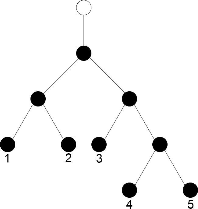
Figure 6.2. A marked $3$-valent tree with its leaves ordered minimally and the corresponding parse tree for the minimal down-split sequence.

6.2.1. Proof of Theorem 1.11 and Theorem 1.12

From 6.13 we are able to easily prove Theorem 1.11 for (unmarked) $3$-valent trees.

Proof.

Let $\mathbf{T}$ be a fixed (unknown) $3$-valent tree with $n$ leaves and let $\mathcal{W}_{\mathbf{T}}$ be its random length sequence. Conditional on $Y_{1}$, $\mathcal{W}_{\mathbf{T}}$ is the modified random length sequence of the marked binary tree $(\mathbf{T},Y_{1})$. Thus, if

$$\operatorname{\mathbb{P}}\{\mathcal{W}_{\mathbf{T}}=s\}>0,$$

then there must be some leaf $v\in\mathbf{T}$ such that

$$\operatorname{\mathbb{P}}\{\mathcal{W}_{(\mathbf{T},v)}=s\}>0.$$

Let $s^{*}$ be the minimal element of the set

$$\{s\text{ down-split }\colon\operatorname{\mathbb{P}}\{\mathcal{W}_{\mathbf{T}}=s\}>0\}.$$

Then $s^{*}$ must be the minimal down-split sequence for $(\mathbf{T},v)$ for at least one leaf $v$ of $\mathbf{T}$. By 6.13 we can reconstruct $(\mathbf{T},v)$ and hence $\mathbf{T}$ from $s^{*}$. ∎

The above argument can be pushed further to prove Theorem 1.12 for $\mathcal{T}$ a random $3$-valent tree.

Proof.

Let $\mathcal{T}$ be a random $3$-valent tree with $n$ leaves and random length sequence $\mathcal{W}_{\mathcal{T}}$.

Given a $3$-valent tree $\mathbf{T}$ with $n$ leaves, let $s^{\mathbf{T}}$ be the minimal element of the set of down-split sequences of the marked $3$-valent trees $(\mathbf{T},v)$ as $v$ ranges over $\mathbf{L}(\mathbf{T})$. We equip the set of $3$-valent tree with $n$ leaves with a total order that, with a slight abuse of notation, we denote by $\prec$ by declaring that $\mathbf{T}^{\prime}\prec\mathbf{T}^{\prime\prime}$ if $s^{\mathbf{T}^{\prime}}\prec s^{\mathbf{T}^{\prime\prime}}$. Note that if $\mathbf{T}^{\prime}\prec\mathbf{T}^{\prime\prime}$, then $\mathbb{P}\{\mathcal{W}_{\mathbf{T}^{\prime}}=s^{\mathbf{T}^{\prime}}\}>0$ and $\mathbb{P}\{\mathcal{W}_{\mathbf{T}^{\prime\prime}}=s^{\mathbf{T}^{\prime}}\}=0$. Now, for each choice of $\mathbf{T}$ we have

$$\mathbb{P}\{\mathcal{W}_{\mathcal{T}}=s^{\mathbf{T}}\}=\sum_{\mathbf{T}^{\prime}}\mathbb{P}\{\mathcal{T}=\mathbf{T}^{\prime}\}\mathbb{P}\{\mathcal{W}_{\mathbf{T}^{\prime}}=s^{\mathbf{T}}\}=\sum_{\mathbf{T}^{\prime}\preceq\mathbf{T}}\mathbb{P}\{\mathcal{T}=\mathbf{T}^{\prime}\}\mathbb{P}\{\mathcal{W}_{\mathbf{T}^{\prime}}=s^{\mathbf{T}}\},$$

and the conclusion that we can recover $\mathbb{P}\{\mathcal{T}=\mathbf{T}\}$ as $\mathbf{T}$ ranges over the $3$-valent trees with $n$ leaves follows simply from the observation that if $b$ is a row vector of length $N$ and $A$ is an $N\times N$ matrix that has all entries below the diagonal zero and all entries on the diagonal strictly positive, then there is a unique row vector $x$ of length $N$ such that $b=xA$. ∎

6.3. Up-split sequences

We now prove Theorem 1.11 and Theorem 1.12 for rooted binary trees. Analogous to the objects we introduced for marked $3$-valent trees, we begin with a definition of a class of sequences that will appear in the support of the random length sequence of a rooted binary tree.

Definition 6.14.

An up-split sequence is an element of the class of increasing sequences of nonnegative integers defined recursively as follows.

The sequence

$$s=(0)$$

is an up-split sequence.

a sequence $s=(s_{1},\ldots,s_{n})$, $n>1$, is an up-split sequence if

$$\{1\leq k<n\colon s_{k}=2k-2\}\neq\emptyset$$

and, setting

$$k_{s}:=\sup\{1\leq k<n\colon s_{k}=2k-2\},$$

• $(s_{1},\ldots,s_{k_{s}})$ is an up-split sequence,

• $(s_{k_{s}+1}-(2k_{s}-1),\ldots,s_{n}-(2k_{s}-1))$ is a down-split sequence.

The index $k_{s}$ is the splitting index of $s$.

Example 6.15.

Suppose that $\mathbf{T}$ is a rooted binary tree with root $o$. In a manner similar to the construction in 6.2 we can order a partial order on $\mathbf{V}(\mathbf{T})$ by declaring that $x$ precedes $y$ if $x\neq y$ is on the path between $\rho$ and $y$, and we can extend this partial order to a total order $<$ such that if $w,x,y,z$ are such that $w$ and $x$ are not comparable in the partial order but $w<x$, $w$ precedes $y$ in the partial order, and $x$ precedes $z$ in the partial order, then $y<z$. Suppose that $y_{1}<y_{2}<\ldots<y_{n}$ is the ordered listing of $\mathbf{L}(\mathbf{T})$. Set $s_{1}:=0$ and $s_{k}:=\mathbf{W}_{\mathbf{T}}(\{y_{1},\ldots,y_{k}\})$, $2\leq k\leq n$. Then $(s_{1},\ldots,s_{n})$ is an up-split sequences. The leaves $y_{1},\ldots,y_{k_{s}}$ and $y_{k_{s}+1},\ldots,y_{n}$ respectively span the two binary subtrees $\mathbf{T}^{\prime}$ and $\mathbf{T}^{\prime\prime}$ that are rooted at the two children of the root $o$. The subtree spanned by $o$ and $y_{k_{s}+1},\ldots,y_{n}$ is a $3$-valent tree.

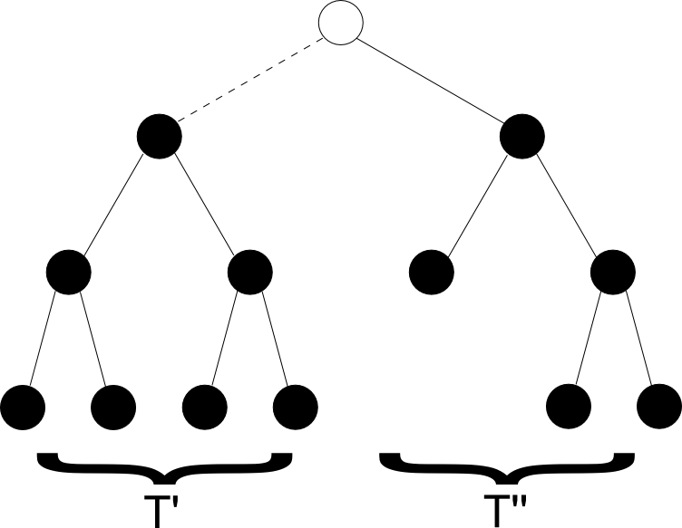
Figure 6.3. A rooted binary tree split as a rooted binary subtree $\mathbf{T}^{\prime}$ and a marked $3$-valent tree $(\mathbf{T}^{\prime\prime},o)$.

The following analogue of Lemma 6.5 is clear from Figure 6.3.

Lemma 6.16.

For every rooted binary tree $\mathbf{T}$, there is at least one up-split sequence $s$ with

$$\operatorname{\mathbb{P}}\{(0,\mathcal{W}_{\mathbf{T}})=s\}>0.$$

The following analogue of Lemma 6.6 can be established using a similar inductive proof.

Lemma 6.17.

If $s=(s_{1},\ldots,s_{n})$ is an up-split sequence then $s_{n}=2n-2$.

Definition 6.18.

Define a total order $\ll$ on the set of up-split sequences of a given length recursively as follows. Firstly, $(0)\ll(0)$ does not hold. Next, let $s$ and $r$ be two up-split sequences indexed by $\{1,\ldots,n\}$ with respective splitting indices $k_{s}$ and $k_{r}$. Set

$$s^{\prime}=\left(s_{1},\ldots,s_{k}\right),\quad r^{\prime}=\left(r_{1},\ldots,r_{k}\right)$$

and

$$s^{\prime\prime}=\left(s_{k+1}-(2k-1),\ldots,s_{n}-(2k-1)\right),\quad r^{\prime\prime}=\left(r_{k+1}-(2k-1),\ldots,r_{n}-(2k-1)\right).$$

Declare that

$$s\ll r$$

if

$$k_{s}>k_{r}$$

or

$$k_{s}=k_{r}\quad\text{and}\quad s^{\prime}\ll r^{\prime}$$

or

$$k_{s}=k_{r}\quad\text{and}\quad s^{\prime}=r^{\prime}\quad\text{and}\quad s^{\prime\prime}\prec r^{\prime\prime}.$$

Remark 6.19.

Note for up-split sequences $s$ and $r$, that $s\ll r$ implies that the splitting index of $s$ is greater than or equal to the splitting index of $r$. For down-split sequences $u$ and $t$, $u\prec t$ implies that the splitting index of $u$ is less than or equal to the splitting index of $t$. This change in the direction of the inequalities matches the switch in the definition of the splitting index from an infimum for down-split sequences to a supremum for up-split sequences.

The next result follows easily by induction.

Lemma 6.20.

The binary relation $\ll$ is a total order on the set of up-split sequences of a given length.

Definition 6.21.

The minimal up-split sequence for a rooted binary tree $\mathbf{T}$ is the minimal element (with respect to the total order $\ll$) of the set

$$\{s\text{ up-split }\colon\operatorname{\mathbb{P}}\{\mathcal{W}_{\mathbf{T}}=s\}>0\}.$$

The up-split sequence analogues of Lemma 6.11 and 6.12 are the following and they are proved in essentially the same manner.

Lemma 6.22.

Given a binary tree $\mathbf{T}$ with root $o$, let $\mathbf{T}^{\prime}$ and $\mathbf{T}^{\prime\prime}$ be the binary subtrees rooted at the two children of $o$. Set

$$m:=\sup\{1\leq k<n\colon\operatorname{\mathbb{P}}\{W_{k}=2k-2\}>0\}.$$

Then $W_{m}=2m-2$ if and only if $Y_{1},\ldots,Y_{m}\in\mathbf{T}^{\prime}$ and $Y_{m+1},\ldots,Y_{n}\in\mathbf{T}^{\prime\prime}$ or vice versa.

Corollary 6.23.

Let $\mathbf{T}$ be a rooted binary tree with random length sequence $\mathcal{W}_{\mathbf{T}}=(W_{2},\ldots,W_{n})$. Then

$$m:=\sup\{1\leq k<n\colon\operatorname{\mathbb{P}}\{W_{k}=2k-2\}>0\}$$

is the splitting index for the minimal up-split sequence for $\mathbf{T}$.

The following analogue of 6.13 for up-split sequences follows from Lemma 6.22 and 6.23 in essentially the same manner that 6.13 followed from Lemma 6.11 and 6.12.

Proposition 6.24.

Let $s$ be the minimal up-split sequence for a rooted binary tree $\mathbf{T}$. There is no other rooted binary tree for which $s$ is the minimal up-split sequence.

Clearly, 6.24 completes the proof of Theorem 1.11. To establish Theorem 1.12 in the case of $\mathcal{T}$ a random rooted binary tree, we need only repeat the argument of the proof of Theorem 1.12 given in Section 6.2.1 for $3$-valent trees.

6.4. $(k+1)$-valent and rooted $k$-ary combinatorial trees

The proof of the extension Theorem 1.11 and Theorem 1.12 to $(k+1)$-valent and rooted $k$-ary combinatorial trees for $k\geq 3$ is very similar to the $k=2$ case and involves the introduction of suitable notion of down-split and up-split sequences along with appropriate total orders on these sets of sequences. The only difference is that both types of split sequences are now split into $k$ smaller sequences, instead of just two. We leave the details to the reader.

7. Open problems

The original conjecture Question 1.1 remains open in general, both for simple trees with arbitrary edge weights (not in general position), and for combinatorial trees. An even more general question is suggested by Theorem 1.12.

Question 7.1.

Let $\mathcal{T}$ be a random tree with probability distribution supported either on the set of simple trees with $n$ leaves and general edge weights or the set of combinatorial trees with $n$ leaves. Can the probability distribution of $\mathcal{T}$ be determined uniquely from the joint probability distribution of the random length sequence $\mathcal{W}_{\mathcal{T}}$?

Even if the answer to Question 7.1 is “no”, the answer may still be “yes” if the probability distribution of $\mathcal{T}$ is known a priori to belong to some particular family of probability distributions. There are, of course, many families of probability models for with random trees with $n$ leaves that are described by a small number of parameters (for example, conditioned Galton-Watson models, the various preferential attachment models), and perhaps the value of these parameters can be determined from the joint probability distribution of the random length sequence of a random tree that is known a priori to be distributed according to a member of one of these families.

Question 7.2.

What are the necessary and sufficient conditions on a vector for there to be an edge-weighted tree $\mathbf{T}$ such that the vector is in the support of $\mathcal{W}_{\mathbf{T}}$?

We remarked in the Introduction that the focus of this paper is superficially similar to that in [KS85], where the problem of reconstructing a combinatorial tree from its number deck (the sizes of the subtrees in the forests produced by deleting each vertex) was studied. The lists of lists that are the number deck of some combinatorial tree are characterized in [KEM86].

Question 7.3.

Are there more parsimonious quantities derived from the joint probability distribution of the random length sequence that still carry a lot of information about $\mathbf{T}$? For example, how much information about $\mathbf{T}$ is contained in the expectation $(\mathbb{E}[W_{2}],\ldots,\mathbb{E}[W_{n}])$ of the random length sequence and is it possible to characterize those vectors which can arise as the expectation of the random length sequence?

References

- [AHU75] Alfred V. Aho, John E. Hopcroft, and Jeffrey D. Ullman, The design and analysis of computer algorithms, Addison-Wesley Publishing Co., Reading, Mass.-London-Amsterdam, 1975, Second printing, Addison-Wesley Series in Computer Science and Information Processing. MR 0413592 (54 #1706)
- [Bed74] A. R. Bednarek, A note on tree isomorphisms, J. Combinatorial Theory Ser. B 16 (1974), 194–196. MR 0332540 (48 #10867)
- [BES12] Shankar Bhamidi, Steven N. Evans, and Arnab Sen, Spectra of large random trees, J. Theoret. Probab. 25 (2012), no. 3, 613–654. MR 2956206
- [BM93] Phillip Botti and Russell Merris, Almost all trees share a complete set of immanantal polynomials, J. Graph Theory 17 (1993), no. 4, 467–476. MR MR1231010 (94g:05053)
- [Bon69] J. A. Bondy, On Kelly’s congruence theorem for trees, Proc. Cambridge Philos. Soc. 65 (1969), 387–397. MR 0260614 (41 #5238)
- [Bon91] by same author, A graph reconstructor’s manual, Surveys in combinatorics, 1991 (Guildford, 1991), London Math. Soc. Lecture Note Ser., vol. 166, Cambridge Univ. Press, Cambridge, 1991, pp. 221–252. MR 1161466 (93e:05071)
- [Bun71] Peter Buneman, The recovery of trees from measures of dissimilarity, Mathematics in the archaeological and historical sciences (F.R. Hodson, D.G. Kendall, and P. Tautu, eds.), Edinburgh University Press, Edinburgh, 1971, pp. 387–395.
- [Bun74] by same author, A note on the metric properties of trees, J. Combinatorial Theory Ser. B 17 (1974), 48–50. MR 0363963 (51 #218)
- [DHM07] A. Dress, K. T. Huber, and V. Moulton, Some uses of the Farris transform in mathematics and phylogenetics—a review, Ann. Comb. 11 (2007), no. 1, 1–37. MR 2311928 (2008a:05072)
- [Diu13] Mircea V. Diudea, Hosoya-Diudea polynomials revisited, MATCH Commun. Math. Comput. Chem. 69 (2013), no. 1, 93–100. MR 3052391
- [EG06] David Eisenstat and Gary Gordon, Non-isomorphic caterpillars with identical subtree data, Discrete Math. 306 (2006), no. 8-9, 827–830. MR 2234989 (2006m:05057)
- [Eva08] Steven N. Evans, Probability and real trees, Lecture Notes in Mathematics, vol. 1920, Springer, Berlin, 2008, Lectures from the 35th Summer School on Probability Theory held in Saint-Flour, July 6–23, 2005. MR MR2351587
- [Fel04] J. Felsenstein, Inferring phylogenies, Sinauer Press, Sunderland, MA, 2004.
- [FGM97] Philippe Flajolet, Xavier Gourdon, and Conrado Martínez, Patterns in random binary search trees, Random Structures Algorithms 11 (1997), no. 3, 223–244. MR 1609509 (98m:68042)
- [GM89] Gary Gordon and Elizabeth McMahon, A greedoid polynomial which distinguishes rooted arborescences, Proc. Amer. Math. Soc. 107 (1989), no. 2, 287–298. MR 967486 (90a:05046)
- [GMOY95] Gary Gordon, Eleanor McDonnell, Darren Orloff, and Nen Yung, On the Tutte polynomial of a tree, Proceedings of the Twenty-sixth Southeastern International Conference on Combinatorics, Graph Theory and Computing (Boca Raton, FL, 1995), vol. 108, 1995, pp. 141–151. MR 1369283 (96j:05036)
- [HLP88] G. H. Hardy, J. E. Littlewood, and G. Pólya, Inequalities, Cambridge Mathematical Library, Cambridge University Press, Cambridge, 1988, Reprint of the 1952 edition. MR 944909 (89d:26016)
- [HP66] Frank Harary and Ed Palmer, The reconstruction of a tree from its maximal subtrees, Canad. J. Math. 18 (1966), 803–810. MR 0200190 (34 #89)
- [HS07] Klaas Hartmann and Mike Steel, Phylogenetic diversity: from combinatorics to ecology, Reconstructing evolution, Oxford Univ. Press, Oxford, 2007, pp. 171–196. MR 2359353
- [Kel57] Paul J. Kelly, A congruence theorem for trees, Pacific J. Math. 7 (1957), 961–968. MR 0087949 (19,442c)
- [KEM86] I. Krasikov, M. N. Ellingham, and Wendy Myrvold, Legitimate number decks for trees, Ars Combin. 21 (1986), 15–17. MR 846676 (87j:05067)
- [KS85] I. Krasikov and J. Schönheim, The reconstruction of a tree from its number deck, Discrete Math. 53 (1985), 137–145, Special volume on ordered sets and their applications (L’Arbresle, 1982). MR 786484 (86d:05088)
- [Lau83] J. Lauri, Proof of Harary’s conjecture on the reconstruction of trees, Discrete Math. 43 (1983), no. 1, 79–90. MR 680306 (83k:05080)
- [Man70] Bennet Manvel, Reconstruction of trees, Canad. J. Math. 22 (1970), 55–60. MR 0256926 (41 #1581)
- [ME11] Frederick A Matsen and Steven N Evans, Ubiquity of synonymity: almost all large binary trees are not uniquely identified by their spectra or their immanantal polynomials., Algorithms for molecular biology: AMB 7 (2011), no. 1, 14–14.
- [MMW08] Jeremy L. Martin, Matthew Morin, and Jennifer D. Wagner, On distinguishing trees by their chromatic symmetric functions, J. Combin. Theory Ser. A 115 (2008), no. 2, 237–253. MR 2382514 (2008m:05115)
- [OS14] Rosa Orellana and Geoffrey Scott, Graphs with equal chromatic symmetric functions, Discrete Math. 320 (2014), 1–14. MR 3147202
- [Pau00] Yves Pauplin, Direct calculation of a tree length using a distance matrix, Journal of Molecular Evolution 51 (2000), no. 1, 41–47.
- [PS04] L. Pachter and D. Speyer, Reconstructing trees from subtree weights, Appl. Math. Lett. 17 (2004), no. 6, 615–621. MR 2064171 (2005b:05066)
- [RC77] Ronald C. Read and Derek G. Corneil, The graph isomorphism disease, J. Graph Theory 1 (1977), no. 4, 339–363. MR 0485586 (58 #5412)
- [RS82] Joseph Rosenblatt and Paul D. Seymour, The structure of homometric sets, SIAM Journal on Algebraic Discrete Methods 3 (1982), no. 3, 343–350.
- [Sch73] Allen J. Schwenk, Almost all trees are cospectral, New Directions in the Theory of Graphs, Academeic Press, New York, 1973, pp. 275–307.
- [SF83] Jean-Marc Steyaert and Philippe Flajolet, Patterns and pattern-matching in trees: an analysis, Inform. and Control 58 (1983), no. 1-3, 19–58. MR 750401 (86h:68070)
- [SP69] J. M. S. Simões Pereira, A note on the tree realizability of a distance matrix, J. Combinatorial Theory 6 (1969), 303–310. MR 0237362 (38 #5650)
- [SS03] Charles Semple and Mike Steel, Phylogenetics, Oxford Lecture Series in Mathematics and its Applications, vol. 24, Oxford University Press, Oxford, 2003. MR 2060009 (2005g:92024)
- [SS04] by same author, Cyclic permutations and evolutionary trees, Adv. in Appl. Math. 32 (2004), no. 4, 669–680. MR 2053839 (2005g:05042)
- [Sta95] Richard P. Stanley, A symmetric function generalization of the chromatic polynomial of a graph, Adv. Math. 111 (1995), no. 1, 166–194. MR 1317387 (96b:05174)
- [Tur68] James Turner, Generalized matrix functions and the graph isomorphism problem, SIAM J. Appl. Math. 16 (1968), 520–526. MR 0228370 (37 #3951)
- [Ula60] S. M. Ulam, A collection of mathematical problems, Interscience Tracts in Pure and Applied Mathematics, no. 8, Interscience Publishers, New York-London, 1960. MR 0120127 (22 #10884)
- [Zar65] K.A. Zaretskii, Constructing trees from the set of distances between pendant vertices, Uspehi Matematiceskih Nauk. 20 (1965), 90–92.