A Convex Optimization Approach to Smooth Trajectories
for Motion Planning with Car-Like Robots

Abstract

In the recent past, several sampling-based algorithms have been proposed to compute trajectories that are collision-free and dynamically-feasible. However, the outputs of such algorithms are notoriously jagged. In this paper, by focusing on robots with car-like dynamics, we present a fast and simple heuristic algorithm, named Convex Elastic Smoothing (CES) algorithm, for trajectory smoothing and speed optimization. The CES algorithm is inspired by earlier work on elastic band planning and iteratively performs shape and speed optimization. The key feature of the algorithm is that both optimization problems can be solved via convex programming, making CES particularly fast. A range of numerical experiments show that the CES algorithm returns high-quality solutions in a matter of a few hundreds of milliseconds and hence appears amenable to a real-time implementation.

I Introduction

The problem of planning a collision-free and dynamically-feasible trajectory is fundamental in robotics, with application to systems as diverse as ground, aerial, and space vehicles, surgical robots, and robotic manipulators [1]. A common strategy is to decompose the problem in steps of computing a collision-free, but possibly highly-suboptimal or not even dynamically-feasible trajectory, smoothing it, and finally reparameterizing the trajectory so that the robot can execute it [2]. In other words, the first step provides a strategy that explores the configuration space efficiently and decides “where to go,” while the subsequent steps provide a refined solution that specifies “how to go.”

The first step is often accomplished by running a sampling-based motion planning algorithm [1], such as PRM [3] or RRT [4]. While these algorithms are very effective for quickly finding collision-free trajectories in obstacle-cluttered environments, they often return jerky, unnatural paths [5]. Furthermore, sampling-based algorithms can only handle rather simplified dynamic models, due to the complexity of exploring the state space while retaining dynamic feasibility of the trajectories. The end result is that the trajectory returned by sampling-based algorithms are characterized by jaggedness and are often dynamically-infeasible, which requires the subsequent use of algorithms for trajectory smoothing and reparametrization.

Accordingly, the objective of this paper is to design a fast and simple heuristic algorithm for trajectory smoothing and reparametrization that is amenable to a real-time implementation, with a focus on mobile robots, in particular robotic cars. Specifically, we seek an algorithm that within a few hundreds of milliseconds can turn a jerky trajectory returned by a sampling-based motion planner into a smooth, speed-optimized trajectory that fulfills strict dynamical constraints such as friction, bounded acceleration, or turning radius limitations.

I-A Literature Review

The problem of smoothing a trajectory returned by a sampling-based planner is not new and has been studied since the introduction of sampling-based algorithms [6]. For planning problems that do not involve the fulfillment of dynamic constraints (e.g., limited turning radius), efficient smoothing algorithms are already available. In this case, the most widely applied method is the Shortcut heuristic, because of its effectiveness and simple implementation [7]. In a typical implementation, this algorithm considers two random configurations along the trajectory. If these two configurations can be connected with a new shorter trajectory (as computed via a local planner), then the original connection is replaced with the new one.

For planning problems with dynamic constraints, however, the situation is more contentious. While several works have studied sampling-based algorithms for kinodynamic planning [4, 8, 9, 10, 11, 12], relatively few works have addressed the issues of trajectory smoothing with dynamic constraints. Broadly speaking, current techniques can be classified into two categories [5], namely shortcut methods and optimization-based methods. Shortcut methods strive to emulate the Shortcut algorithm in a kinodynamic context. Specifically, jerky portions of a path are replaced with curve segments such as parabolic arcs [13], clothoids [14], Bézier curves [15], Catmull-Rom splines [16], cubic B-splines [5], or Dubins curves [17]. Such methods are rather fast (they usually complete in a few seconds), but handle dynamic constraints only implicitly, for example, by constraining the curvature of the trajectories and/or ensuring $C^{2}$ continuity. Also, they usually do not involve speed optimization along the computed trajectory. Notably, two of the main teams in the DARPA Grand Challenge, namely team Stanford [18] and team CMU [19], applied shortcut methods as their smoothing procedure.

In contrast, optimization-based methods handle dynamic constraints explicitly, as needed, for example, for high-performance mobile vehicles. Two common approaches are gradient-based methods [20] and elastic bands or elastic strip planning [21, 22, 23], which model a trajectory as an elastic band. These works, however, are mostly geared toward robotic manipulators [22], may still require several seconds to find a solution [20], and generally do not address speed optimization along the trajectory.

I-B Statement of Contributions

In this paper, leveraging recent strides in the field of convex optimization [24], we design a novel algorithm, named Convex Elastic Smoothing (CES) algorithm, for trajectory smoothing and speed optimization. The focus is on mobile robots with car-like dynamics. Our algorithm is inspired by the elastic band approach [23], in that we identify a collision-free “tube” around the trajectory returned by a sampling-based planner, within which the trajectory is “stretched” and speed is optimized. The stretching and speed optimization steps rely on convex optimization. In particular, the stretching step draws inspiration from [25], while the speed optimization step is essentially an implementation of the algorithm in [26]. In contrast with [23], our algorithm uses convex optimization for the stretching process, performs speed optimization, and handles a variety of constraints (e.g., friction) that were not considered in [23]. As compared to [25], our algorithm handles more general workspaces and removes the assumption of a constant speed.

Specifically, the CES algorithm divides the trajectory smoothing process into two steps: (1) given a fixed velocity profile along a reference trajectory, optimize the shape of the trajectory, and (2) given a fixed shape for the trajectory, optimize the speed profile along the trajectory. We show that each of the two steps can be readily solved as a convex optimization problem. The two steps are then repeated until a termination criterion is met (e.g., timeout). In this paper, the initial reference trajectory is computed by running the differential FMT^∗ algorithm [27], a kinodynamic variant of the FMT^∗ algorithm [28]. Numerical experiments on a variety of scenarios show that in a few hundreds of milliseconds the CES algorithm outputs a “high-quality” trajectory, where the jaggedness of the original trajectory is eliminated and speed is optimized. Coupled with differential FMT^∗, the CES algorithm is able to find high-quality solutions to rather complicated planning problems in well under a second, which appears promising for a real-time implementation.

We mention that the reference trajectory used as an input to the CES algorithm can be the output of any sampling-based motion planner, and indeed of any motion planning algorithm. In particular, the CES algorithm appears to perform well even when the reference trajectory is not collision-free or does not fulfill some of the dynamic constraints (see Section IV for more details). Also, while in this paper we mostly focus on vehicles with second-order, car-like dynamics, the CES algorithm can be generalized to a variety of other mobile systems such as aerial vehicles and spacecraft.

I-C Organization

This paper is structured as follows. In Section II we formally state the problem we wish to solve. In Section III we present the CES algorithm, a novel algorithm for trajectory smoothing that relies on convex optimization and runs in a few hundreds of milliseconds. In Section IV we present results from numerical experiments highlighting the speed of the the CES algorithm and the quality of the returned solutions. Finally, in Section V, we draw some conclusions and discuss directions for future work.

II Problem Statement

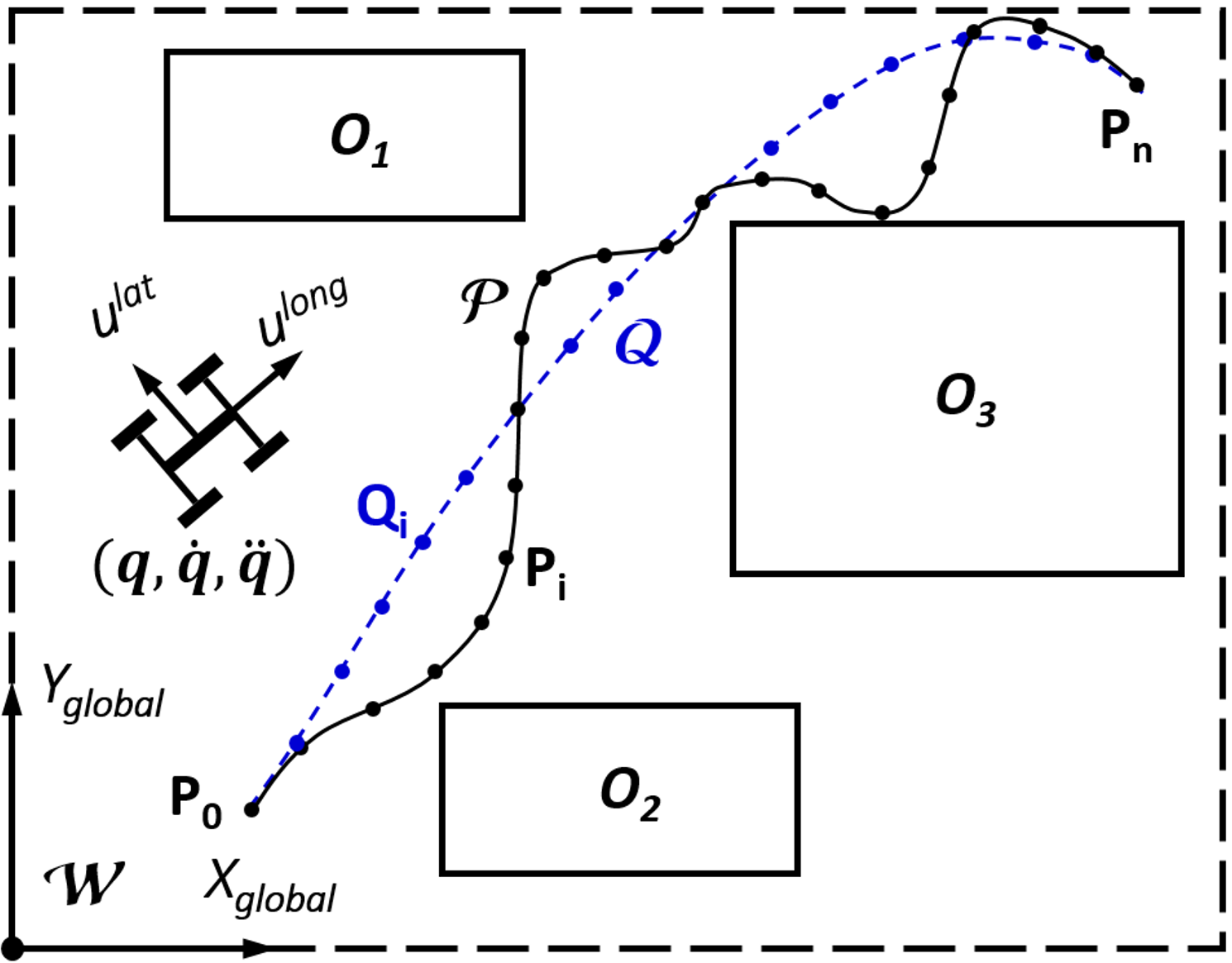
Let $\mathcal{W}\subset{\mathbb{R}}^{2}$ denote the two-dimensional work space for a car-like vehicle. Let $\mathcal{O}=\{O_{1},O_{2},\ldots,O_{m}\}$, with $O_{i}\subset\mathcal{W}$, $i=1,\ldots,m$, denote the set of obstacles. For simplicity, we assume that the obstacles have polygonal shape. In this paper we primarily focus on a unicycle dynamic model for the vehicle. Extensions to more sophisticated car-like models are discussed in Section IV. Specifically, following [26], let $\mathbf{q}\in\mathcal{W}$ represent the position of the vehicle, and $\mathbf{\dot{q}}$ and $\mathbf{\ddot{q}}$ its velocity and acceleration, respectively. We consider a non-drifting and non-reversible car model so that the heading of the vehicle is the same as the direction of the instantaneous velocity vector, and we denote by $\phi(\mathbf{\dot{q}})$ the mapping from vehicle’s speed to its heading. The control input $\mathbf{u}=[u^{\mathrm{long}},u^{\mathrm{lat}}]$ is two-dimensional, with the first component, $u^{\mathrm{long}}$, representing longitudinal force and the second component, $u^{\mathrm{lat}}$, representing lateral force. The dynamics of the vehicle are given by

$$m\,\mathbf{\ddot{q}}=\begin{bmatrix}\cos\phi(\mathbf{\dot{q}})&-\sin\phi(\mathbf{\dot{q}})\\[3.00003pt] \sin\phi(\mathbf{\dot{q}})&\cos\phi(\mathbf{\dot{q}})\end{bmatrix}\,\mathbf{u},$$ (1)

where $m$ is the vehicle’s mass, see Figure 1. We consider a friction circle constraint for $\mathbf{u}$, namely

$$\|\mathbf{u}\|\leq\mu\,m\,g,$$ (2)

where $\mu$ is the friction coefficient and $g$ is the gravitational acceleration (in this paper, norms should be interpreted as 2-norms). The longitudinal force is assumed to be upper bounded as

$$u^{\mathrm{long}}\leq\bar{U}^{\mathrm{long}},$$ (3)

where $\bar{U}^{\mathrm{long}}\in{\mathbb{R}}_{>0}$ encodes the force limit from the wheel drive. Finally, we assume a minimum turning radius $R_{\mathrm{min}}$ for the vehicle, which, in turn, induces a constraint on the lateral force according to

$$u^{\mathrm{lat}}\leq m\frac{\|\mathbf{\dot{q}}\|^{2}}{R_{\mathrm{min}}}.$$ (4)

The minimum turning radius ($R_{\mathrm{min}}$) depends on specific vehicle parameters such as wheelbase and maximum steering angle for steering wheels.

Some comments are in order. First, the unicycle model assumes that the heading of the vehicle is the same as the direction of the instantaneous velocity vector. This is a reasonable assumption in most practical situations, but becomes a poor approximation at high speeds when significant under-steering takes place, or at extremely low speeds when the motion is determined by Ackermann steering geometry. We will show, however, that the results presented in this paper can be extended to more complex car models, e.g., half-car models, by leveraging differential flatness of the dynamics. Second, we assume that the actual control inputs such as steering and throttle opening angles can be mapped to $\mathbf{u}$ via a lower-level control algorithm. This is indeed true for most ground vehicles, see, e.g., [29]. Third, the friction circle model captures the dependency between lateral and longitudinal forces in order to prevent sliding. Fourth, constraint (3) might yield unbounded speeds. This issue could be addressed by conservatively choosing a smaller value of $\bar{U}^{\mathrm{long}}$ that guarantees an upper bound of the achievable speed within the planning distance. An alternative formulation is to set a limit on the total traction power $u^{\mathrm{long}}\ \|\mathbf{\dot{q}}\|\leq W$, where $W$ denotes the maximum power provided by the engine. This form is closer to the real constraint on traction force, but it makes the constraint non-convex – this is a topic left for future research. Finally, the model (1)-(4), with minor modifications, can be applied to a variety of other vehicles and robotic systems, e.g., spacecraft, robotic manipulators, and aerial vehicles [26]. Hence, the algorithm presented in this paper may be applied to a rather large class of systems – this is a topic left for future research.

We are now in a position to state the problem we wish to solve in this paper. Consider a collision-free reference trajectory computed, for example, by running a sampling-based motion planner [1]. Let this trajectory be discretized into a set of waypoints $\mathcal{P}:=\{P_{0},P_{1},\ldots,P_{n}\}$, where, by construction, $P_{i}\in\mathcal{W}\setminus\mathcal{O}$ for $i=1,\ldots,n$. The goal is to design a heuristic smoothing algorithm that uses the information about the vehicle’s model (1)-(4), obstacle set $\mathcal{O}$, and (discretized) reference trajectory $\mathcal{P}$ to compute a dynamically-feasible (with respect to model (1)-(4)), collision-free, and smooth trajectory that goes from $P_{0}$ to $P_{n}$ and has an optimized speed profile, see Figure 1. Our proposed algorithm is named CES and is presented in the next section.

Figure 1: The goal of this paper is to design a fast algorithm to locally optimize the output of a motion planner, with a focus on car models. Specifically, the smoothing algorithm takes as input a reference trajectory $\mathcal{P}$ and returns a smoothed trajectory $\mathcal{Q}$ with an optimized speed profile.

III The CES Algorithm

At a high level, the CES algorithm performs the following operations. First, a sequence of “bubbles” is placed along the reference trajectory in order to identify a region of the workspace that is collision free. Such a region can be thought of as a collision-free “tube” within which the reference trajectory, imagined as an elastic band, can be stretched so as to obtain a smoother trajectory. Assuming that a speed profile along the reference trajectory is given, such stretching procedure can be cast as a convex optimization problem, as it will be shown in Section III-B. Furthermore, optimizing the speed profile along a stretched trajectory can also be cast as a convex optimization problem. However, jointly stretching a trajectory and optimizing the speed profile is a non-convex problem. Hence, the CES algorithm proceeds by alternating trajectory stretching and speed optimization. Simulation results, presented in Section IV, show that such a procedure is amenable to a real-time implementation and yields suboptimal, yet high-quality trajectories. Our CES algorithm is inspired by the elastic band and bubble method [23]. The work in [23], however, mostly focuses on geometric (i.e., without differential constraints) planning, and does not consider speed optimization, as opposed to our problem setup.

In the remainder of this section we present the different steps of the CES algorithm, namely, bubble generation, elastic stretching and speed optimization. Finally the overall CES algorithm is presented.

III-A Bubble Generation

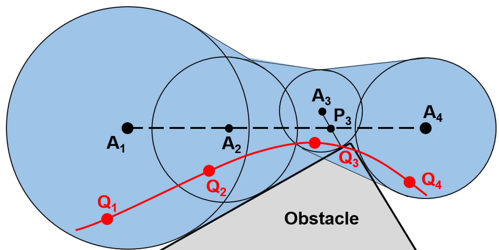
The first step is to compute a sequence of bubbles, one for each waypoint $P_{i}$, so as to identify a collision-free tube along the reference trajectory for subsequent optimization. Since the problem is two-dimensional, each bubble is indeed a circle. As discussed, extensions to systems in higher dimensions (e.g., airplanes or quadrotors) are possible, but are left for future research. The bubble generation algorithm is shown in Algorithm 1.

Algorithm 1 Bubble generation

0  Reference trajectory $\mathcal{P}$, obstacle set $\mathcal{O}$, bubble bounds $r_{l}$ and $r_{u}$

1  for  $i=2:(n-1)$  do

2     if $\|P_{i}-A_{i-1}\|<0.5\cdot r_{i-1}$ then

3        $\mathcal{B}_{i}\leftarrow\mathcal{B}_{i-1}$

4        $A_{i}\leftarrow A_{i-1}$

5        $r_{i}\leftarrow r_{i-1}$

6        $\bf{continue}$

7     end if

8     $\mathcal{B}_{i}\leftarrow\texttt{GenerateBubble}(P_{i})$

9     $r_{i}\leftarrow$ Radius of $\mathcal{B}_{i}$

10     $A_{i}\leftarrow P_{i}$

11     if $r_{i}<r_{l}$ then

12        $\mathcal{B}_{i}\leftarrow\texttt{TranslateBubble}(A_{i},r_{i})$

13        $r_{i}\leftarrow$ Radius of $\mathcal{B}_{i}$

14        $A_{i}\leftarrow$ Center of $\mathcal{B}_{i}$

15     end if

16  end for

Let $\mathcal{B}_{i}$ denote the bubble associated with waypoint $P_{i}$, $i=1,\ldots,n$, and $A_{i}$ and $r_{i}$ denote, respectively, its center and radius. According to this notation, $\mathcal{B}_{i}=\{x\in\mathcal{W}\,|\,\|x-A_{i}\|\leq r_{i}\}$. For each waypoint $P_{i}$, Algorithm 1 attempts to compute a bubble such that: (1) its radius is upper bounded by $r_{u}\in{\mathbb{R}}_{>0}$, (2) whenever possible, its radius is no less than $r_{l}\in{\mathbb{R}}_{>0}$, and (3) its center is as close as possible to $P_{i}$. The role of the upper bound $r_{u}$ is to limit the smoothing procedure within a relatively small portion of the workspace, say 10% (in other words, to make the optimization “local”). In turn, the minimum bubble radius $r_{l}$ is set according to the maximum distance between adjacent waypoints, so that every bubble overlaps with its neighboring bubbles and the placement of new waypoints for trajectory stretching (see Section III-B) does not have any “gaps”.

First, in lines (2)-(7), the algorithm checks whether $P_{i}$ is “too close” to the center of bubble $\mathcal{B}_{i-1}$. If this is the case, bubble $\mathcal{B}_{i}$ is made equal to bubble $\mathcal{B}_{i-1}$. Otherwise, the algorithm considers as candidate center for bubble $\mathcal{B}_{i}$ the waypoint $P_{i}$ (that is collision-free) and computes, via function GenerateBubble($P_{i}$), the largest bubble centered at $P_{i}$ that is collision-free (with maximum radius $r_{u}$), see lines (8)-(10). For rectangular-shaped obstacles, this is a straightforward geometrical procedure. If the obstacles have more general polygonal shapes, a bisection search is performed with respect to the bubble radius. Should the resulting radius be lower than the threshold $r_{l}$, an attempt is made to translate $A_{i}$ so that a larger (collision-free) bubble can be placed, lines (11)-(15). Specifically, function $\texttt{TranslateBubble}(A_{i},r_{i})$ first identifies the edge of the obstacle closest to $A_{i}$ (recall that the obstacles are assumed of polygonal shape). Then, the outward normal direction to the edge is computed and the center of the bubble is moved along such direction until a ball of radius $r_{l}$ can be placed. Should this not be possible, then $\texttt{TranslateBubble}(A_{i},r_{i})$ returns the ball of largest radius among the balls whose centers lie on the aforementioned normal direction.

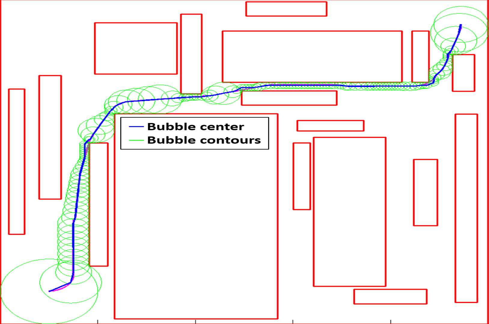
Figure 2 shows an example application of the bubble generation algorithm. The centers $A_{1}$, $A_{2}$ and $A_{4}$ coincide with their corresponding waypoints, while center $A_{3}$ is translated away from waypoint $P_{3}$ to allow for a larger bubble radius. Figure 3 shows a typical output of Algorithm 1.

By construction, the bubble regions are collision-free and represent the feasible space for the placement of new optimized waypoints during the elastic stretching process. Note that in some cases trajectories connecting points in adjacent bubbles may be in collision with obstacles, as shown in Figure 2. This issue is mitigated in practice by considering a “large enough” number of reference waypoints (possibly adding them iteratively) and/or inflating the obstacles. A principled way to select the number of waypoints would rely on a reachability analysis for the unicycle model (1)-(4). However, to minimize computation time, we rely on a heuristic choice for the waypoint number. Specifically, the spacing between the waypoints is roughly equal to a quarter of the car length.

Figure 2: Example application of the bubble generation procedure, Algorithm 1.

Figure 3: Typical output of Algorithm 1 for an environment with rectangular-shaped obstacles.

III-B Elastic Stretching (aka Shape Optimization)

Figure 4: Artificial tensile forces and balance force for a sequence of points placed in bubbles $k-1$, $k$, $k+1$.

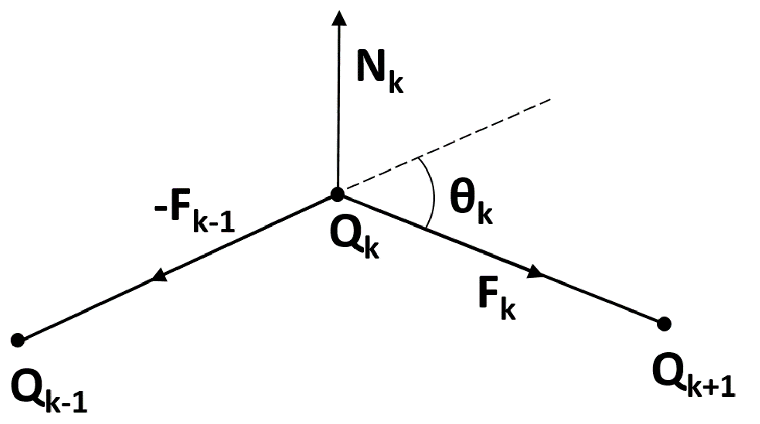
The key insight of the elastic stretching procedure is to view a trajectory as an elastic band, with $n$ nodal points whose positions can be adjusted within the respective (collision-free) bubbles. Such nodal points represent the new waypoints for the smoothed trajectory, which replace the original waypoints in $\mathcal{P}$. Within this perspective, the dynamic constraints on the shape of a trajectory are mimicked by the bending stiffness of the band.

Specifically, consider Figure 4. Let $Q_{k}$ and $Q_{k+1}$ be points, respectively, in bubbles $k$ and $k+1$, with $k=1,\ldots,n-1$. We consider an artificial tensile force $\mathbf{F}_{k}$ between $Q_{k}$ and $Q_{k+1}$ given by

$$\vspace{-.5em}\mathbf{F}_{k}:=Q_{k+1}-Q_{k}.\vspace{-.2em}$$

Accordingly, the balancing force at point $Q_{k}$, $k=1,\ldots,n$ is

$$\vspace{-.5em}\mathbf{N}_{k}:=\mathbf{F_{k-1}}-\mathbf{F_{k}}.$$ (5)

As in [23], the physical interpretation is a series of springs between the bubbles. From a geometric standpoint, the balancing force $\mathbf{N}_{k}$ captures curvature information along a trajectory. Note that if all balance forces are equal to zero, the trajectory is a straight line, which, clearly, has “ideal smoothness.” To smooth a trajectory, the goal is then to place new waypoints $Q_{1},\ldots,Q_{n}$ within the bubbles so as to minimize the sum of the norms of the balance forces subject to constraints due to the vehicle’s dynamics. In this way, the trajectory is “bent” as little as possible in order to avoid collisions with obstacles.

The constraints for the placement of the new waypoints rely on a number of approximations to ensure convexity of the optimization problem. Specifically, assume the longitudinal force $u^{\mathrm{long}}_{k}$ and velocity $\mathbf{v_{k}}$ are given at each waypoint in $\mathcal{P}$ (their optimization will be discussed in the next section). We define $R_{k}$ as the instantaneous turning radius for the car at the $k$th waypoint. The lateral acceleration $\mathbf{a}^{\mathrm{lat}}$ for waypoints $Q_{k}$, $k=2,\ldots,n-1$ can be upper bounded as

$$\mathbf{a}^{\mathrm{lat}}=\frac{\|\mathbf{v_{k}}\|^{2}}{R_{k}}\leq\sqrt{\left(\mu\,g\right)^{2}-\left(\frac{u^{\mathrm{long}}_{k}}{m}\right)^{2}}:=\alpha_{k},$$ (6)

where the inequality follows from the friction circle constraint (2). Hence, $1/R_{k}\leq\alpha_{k}/\|\mathbf{v_{k}}\|^{2}$. To relate $R_{k}$ with $\|\mathbf{N}_{k}\|$, we make use of the following approximations, valid when the waypoints are uniformly spread over a trajectory and dense “enough”: (1) $\|\mathbf{F}_{k}\|\cong\|\mathbf{F}_{k-1}\|$, (2) $\theta_{k}$ is small, and (3) $\theta_{k}\cong\|Q_{k+1}-Q_{k}\|/R_{k}$. Then one can write

$$\begin{split}\|\mathbf{N}_{k}\|&=\|\mathbf{F}_{k-1}-\mathbf{F}_{k}\|\cong 2\cdot\|\mathbf{F}_{k}\|\cdot\sin(\theta_{k}/2)\\ &\cong\|Q_{k+1}-Q_{k}\|\,\theta_{k}\cong\|Q_{k+1}-Q_{k}\|^{2}/R_{k}\\ \ &\leq\|Q_{k+1}-Q_{k}\|^{2}\,\alpha_{k}/\|\mathbf{v_{k}}\|^{2}.\end{split}$$ (7)

Lastly, to make the above inequality a quadratic constraint in the $Q_{k}$’s variables, we approximate the length of each band $Q_{k+1}-Q_{k}$ as the average length $d$ along the reference trajectory, i.e.,

$$d:=\frac{\sum_{k=1}^{n-1}\|P_{k+1}-P_{k}\|}{n-1}.$$

Note that the minimization of $\|\mathbf{N}_{k}\|$ as the optimization objective inherently reduces the non-uniformity of the lengths of each band, which justifies the above approximation.

In summary, we obtain the friction constraint

$$\|\mathbf{N}_{k}\|\leq\alpha_{k}\,\left(\frac{d}{||\mathbf{v}_{k}||}\right)^{2}.$$ (8)

Also, again leveraging equation (7), we obtain the turning radius constraint

$$\|\mathbf{N}_{k}\|\leq\frac{d^{2}}{R_{\mathrm{min}}}.$$ (9)

To constrain the initial and final endpoints of the trajectory, one simply imposes $Q_{1}=P_{1}$ and $Q_{n}=P_{n}$. In turn, to constrain the initial and final heading angles, one can use the constraints $Q_{2}=P_{1}+d\cdot\frac{\mathbf{v}_{1}}{\|\mathbf{v}_{1}\|}$ and $Q_{n-1}=P_{n}-d\cdot\frac{\mathbf{v_{n-1}}}{\|\mathbf{v_{n-1}}\|}$. Noting that $\mathbf{N}_{k}=2Q_{k}-Q_{k-1}-Q_{k+1}$, the elastic stretching optimization problem is:

$$\min_{Q_{3},\ldots,Q_{n-2}} \sum_{k=2}^{n-1}\|2Q_{k}-Q_{k-1}-Q_{k+1}\|^{2}$$

$$\mathrm{s.t.}\qquad \mkern-36.0muQ_{1}=P_{1},\ Q_{2}=P_{1}+d\cdot\frac{\mathbf{v}_{1}}{\|\mathbf{v}_{1}\|}$$

$$\mkern-36.0muQ_{n}=P_{n},\ Q_{n-1}=P_{n}-d\cdot\frac{\mathbf{v}_{n-1}}{\|\mathbf{v}_{n-1}\|}$$

$$\mkern-36.0muQ_{k}\in\mathcal{B}_{k},\quad k=3,\ldots,n-1$$

$$\mkern-36.0mu{\small\|2Q_{k}-Q_{k-1}-Q_{k+1}\|\leq\min\left\{\frac{d^{2}}{R_{\mathrm{min}}},\,\alpha_{k}\left(\frac{d}{\mathbf{v}_{k}}\right)^{2}\right\}}$$

$$\qquad\text{for }k=2,\ldots,n-1.$$

This is a convex optimization problem with quadratic objective and quadratic constraints (QCQP), where the decision variables are the intermediate waypoints $Q_{k}$, $k=3,\ldots,n-2$, which can be placed anywhere within the collision-free regions $\{\mathcal{B}_{3},\ldots,\mathcal{B}_{n-2}\}$,

Note that any feasible solution to the above QCQP, output as a sequence of discrete waypoints, represents a continuous-time trajectory satisfying the unicycle model (1)-(4). This full trajectory may be recovered by interpolating between adjacent waypoints $Q_{k}$,$Q_{k+1}$ using circular arcs centered at the intersection of $\mathbf{v}_{k}^{\perp},\mathbf{v}_{k+1}^{\perp}$, or a straight line if the two velocity vectors are parallel. The speed profile along this continuous trajectory may be taken as piecewise linear, and the discrete constraints (8) and (9) ensure that the continuous constraints (2)-(4) are satisfied. The quality of such trajectories will be investigated in Section IV.

III-C Speed Optimization

The speed optimization over a fixed trajectory relies on the convex optimization algorithm presented in [26]. The inputs to this algorithm are (1) a sequence of waypoints $\{Q_{1},\ldots,Q_{n}\}$ (representing the trajectory to be followed), (2) the friction coefficient $\mu$ for the friction circle constraint in equation (2), and (3) the maximum traction force $\bar{U}^{\mathrm{long}}$ defined in equation (3). The outputs are (1) the sequence of velocity vectors $\{\mathbf{v}_{1},\ldots,\mathbf{v}_{n}\}$ and (2) the sequence of longitudinal control forces $\{u^{\mathrm{long}}_{1},\ldots,u^{\mathrm{long}}_{n}\}$, one for each waypoint $Q_{k}$, $k=1,\ldots,n$. We refer the reader to [26] for details about the algorithm.

III-D Overall Algorithm

The CES algorithm alternates between elastic stretching (Section III-B) and speed optimization (Section III-C), until a given tolerance on length reduction, traversal time reduction, or a timeout condition are met. Note that at iteration $i\geq 2$, the elastic stretching algorithm should use as estimate for the average band length the quantity

$$d^{[i]}:=\frac{\sum_{k=1}^{n-1}\left\|Q^{[i-1]}_{k+1}-Q^{[i-1]}_{k}\right\|}{n-1},$$

where the $Q_{k}^{[i-1]}$’s are the waypoints computed at iteration $i-1$. According to our discussion in Section III-B, at iteration $i=1$ one should set $Q_{k}^{[0]}=P_{k}$, for $k=1,\ldots,n$.

IV Numerical Experiments

In this section we investigate the effectiveness of the CES algorithm along two main dimensions: (1) quality of the smoothed trajectory, measured in terms of traversal time reduction with respect to the reference trajectory, and (2) computation time. We consider three sets of experiments. In the first set, we consider 24 random mazes with rectangular-shaped obstacles, similar to the example in Figure 3. The reference trajectory is computed by running the differential FMT^∗ algorithm [27]. In the second set, to test the robustness of the algorithm, we consider a scenario where the reference trajectory is computed disregarding the vehicle’s dynamics. This could be the case when, to minimize computation time as much as possible, the use of a motion planner is avoided. Finally, we consider a scenario where a robotic car is modeled according to a more sophisticated bicycle (equivalently, half-car) model. The reference trajectory is computed by running differential FMT^∗ on the unicycle model (1)-(4). By leveraging the differential flatness of the bicycle model, the CES algorithm is then applied to the trajectory returned by differential FMT^∗ (computed on a different model). This scenario represents the typical case whereby one seeks to run a motion planner on a simpler model of a vehicle, and then a smoothing algorithm on a more refined model. Furthermore, this scenario shows how to apply the CES algorithms to vehicle models more general than (1)-(4). For all scenarios, the algorithm is stopped whenever the traversal time at the current iteration is no longer reduced with respect to the previous iteration. For the bubble generation method, we chose $r_{u}=10\ m$ and $r_{l}=1\ m$, consistent with the workspace dimensions discussed below.

All numerical experiments were performed on a computer with an Intel(R) Core(TM) i7-3632QM, 2.20GHz processor and 12GB RAM. The CES algorithm was implemented in Matlab with an interface to FORCES Pro [30] for elastic stretching and MTSOS [26] for speed optimization.

IV-A Random Mazes

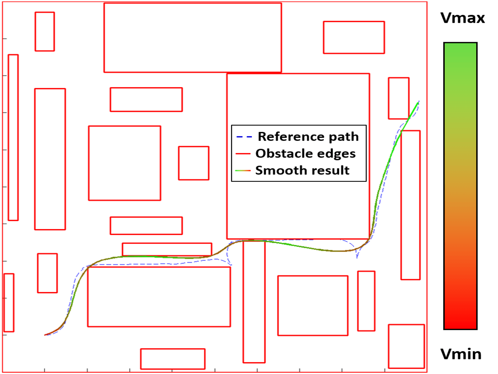
In this scenario the workspace is a $100m\times 100m$ square with rectangular-shaped obstacles randomly placed within (the obstacle coverage was roughly 50%). The parameters for the model in equations (1)-(4) are $m=833$ $kg$, $\mu=0.8$, and $\bar{U}^{\mathrm{long}}=0.5$ $\mu mg$. The reference trajectories, computed via differential FMT^∗ by using 1,000 samples, were discretized into 257 waypoints with an average segment length equal to $0.56$ $m$. On average, each iteration (consisting of bubble generation, shape optimization, and speed optimization) required 119 ms, with a standard deviation of 14 ms. Specifically, the bubble generation algorithm required, on average, 26ms. The shape optimization algorithm required 74 ms. Finally, the speed optimization required 19 ms. A typical smoothed trajectory is portrayed in Figure 5. The traversal time reduction, which is computed according to the formula $\frac{t_{\mathrm{initial}}-t_{\mathrm{final}}}{t_{\mathrm{initial}}}\cdot 100\%$, ranges from a minimum of 0.2% to a maximum of 18%, with the average value being $3.54\%$. Figure 5 shows the smoothed trajectory for one of the 24 random mazes. We note that, apart from the benefit of reduction of traversal time, a smoothed trajectory may be easier to track for a lower-level controller.

Figure 5: A typical smoothed trajectory for the random maze scenario. In this case, the traversal time reduction is $9.12\%$.

IV-B Lane Changing

For this scenario, we consider a road lane 50 $m$ long with rectangular-shaped obstacles in it. The parameters for the model in equations (1)-(4) are $m=1,725$ $kg$, $\mu=0.5$, and $\bar{U}^{\mathrm{long}}=0.3$ $\mu mg$. The reference trajectory is generated by simply computing the center line of the collision-free “tube” along the road. This corresponds to the case where, to minimize computation time as much as possible, a reference trajectory is computed disregarding vehicle’s dynamics. Figure 6 shows the smoothed trajectory and speed profile. The computation time was $100$ ms. This scenario illustrates that algorithm CES can also smooth reference trajectories that are not dynamically-feasible. Of course, in this case the traversal time for the smoothed trajectory is longer, due to the dynamic constraints.

Figure 6: Smoothed trajectory for the lane changing scenario.

IV-C Smoothing with Bicycle Model

In this scenario, we assume a more sophisticated model for the vehicle, namely a half-car (or bicycle) model, see Figure 7. This model is widely used when local vehicle states such as sideslip angle and yaw rate are of primary interest [29]. In Figure 7, $\mathbf{p}_{cg}$ denotes the center of gravity (CG) of the car, $\psi$ denotes vehicle’s orientation, and $v_{x}$ and $v_{y}$ denote components of speed $\mathbf{v}$ in a body-fixed axis system. Also, $l_{f}$ and $l_{r}$ denote the distances from the CG to the front and rear wheels, respectively. Finally, $F_{\alpha\beta}$, with $\alpha\in\{f,r\},\beta\in\{x,y\}$ denotes the frictional forces of front and rear wheels. The control input is represented by the triple $\zeta=[\delta,s_{fx},s_{rx}]$, where $\delta$ denotes the steering angle of the front wheel, and $s_{fx}$ and $s_{rx}$ denote the longitudinal slip angles of the front and rear tires, respectively. See [31] for more details. Referring to Figure 7, the position $\mathbf{p}_{co}$ can be used as a differentially flat output [32]. Specifically, let $m$ be the mass of the vehicle, $I_{z}$ the yaw moment of inertia, and $l_{co}:=I_{z}/ml_{r}$. One can show that

$$m\ \mathbf{\ddot{p}_{co}}=m\ R(\psi)\begin{bmatrix}\dot{v_{x}}-v_{y}\dot{\psi}-l_{co}\dot{\psi}^{2}\\[3.00003pt] \dot{v_{y}}+v_{x}\dot{\psi}+l_{co}\ddot{\psi}\end{bmatrix}:=R(\psi)\mathbf{u},$$

where $R(\cdot)$ is the 2D rotation matrix and $\mathbf{u}=[u^{\mathrm{long}},u^{\mathrm{lat}}]$ is the flat input comprising longitudinal force $u^{\mathrm{long}}$ and latitudinal force $u^{\mathrm{lat}}$. Note that the flat dynamics are formally identical to those of the unicycle model (1)-(4). By leveraging differential flatness, the idea is then to smooth a trajectory in the flat output space and then map the flat input $\mathbf{u}$ to the input $\zeta=[\delta,s_{fx},s_{rx}]$. Constraints for the flat input $\mathbf{u}$ take the same form as in equations (2)-(4) – the details can be found in [31]. When mapping $\mathbf{u}$ into $[\delta,s_{fx},s_{rx}]$, under a no-drift assumption, only two real inputs can be uniquely determined, while the third is effectively a “degree of freedom,” see [31, Section II]. In this paper, we consider as degree of freedom the real input $s_{rx}$. Its value is set equal to the solution of an optimization problem aimed at minimizing the tracking error with respect to the trajectory obtained with the flat input $\mathbf{u}$ (the tracking error is due to the no-drift assumption).

Figure 7: Definition of variables for bicycle model (adapted from [31]).

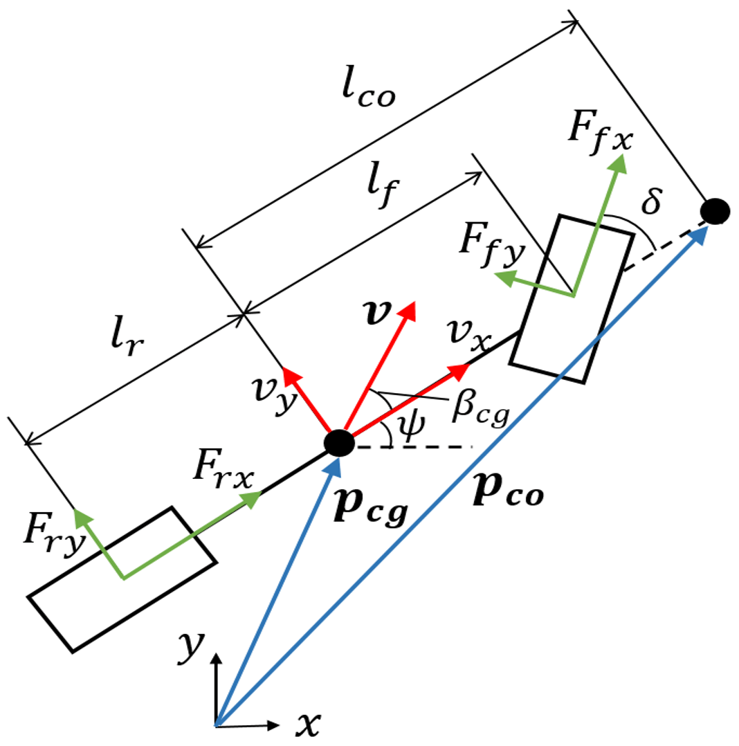
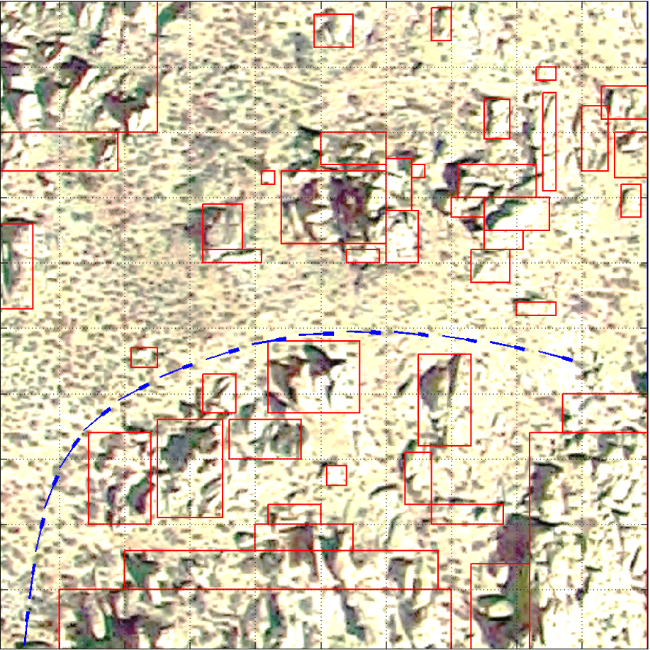
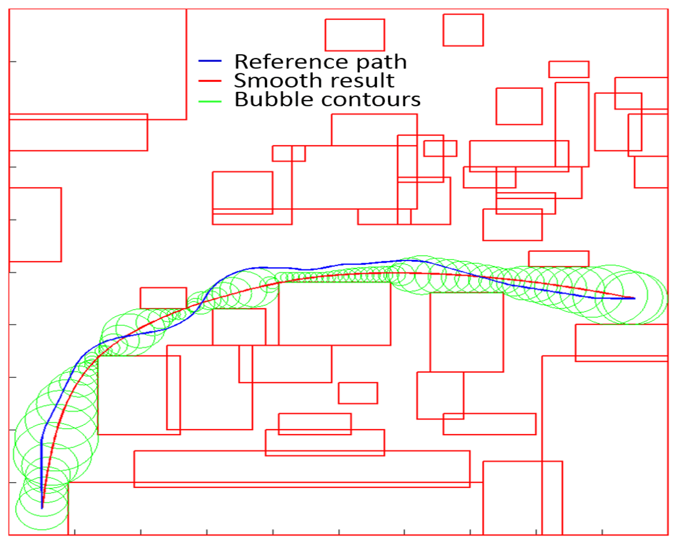
Figure 9 shows the application of the CES algorithm to a $100m\times 100m$ rocky terrain portrayed in Figure 8. The parameters of the bicycle model are $m=1,725$ $kg$, $I_{z}=1,300$ $kg\cdot m^{2}$, $l_{f}=1.35$ $m$, $l_{r}=1.15$ $m$, and $h=0.3$ $m$. In this case, the reference trajectory is computed by running differential FMT^∗ with 1,000 samples on a unicycle model, as defined in equations (1)-(4). The reference trajectory is discretized into 257 waypoints. The CES algorithm is then applied by using the aforementioned bicycle model and differential flatness transformation. Interestingly, in this example the smoothing algorithm is applied to a reference trajectory generated with a different (simpler) model – this, again, shows the robustness of the proposed approach. The length reduction was 4.19%, while the traversal time reduction was 39.74%. Computation times are reported in Table I. Considering two iterations, the total smoothing time is 798 ms. Specifically, about 30% of the time is taken by differential FMT^∗, 20% by the shape optimization algorithm, and the remaining time by the bubble generation, the speed optimization, and the mapping via differential flatness to a bicycle model. Remarkably, this result appears compatible with the real-time requirements of autonomous driving. Indeed, we note that the example in Figure 9 is rather extreme in that a very long trajectory is planned amid several obstacles. In practical scenarios (e.g., urban driving), the planning problem may be simpler, implying that the computation times would be even lower.

IV-D Elastic Stretching Moose Test

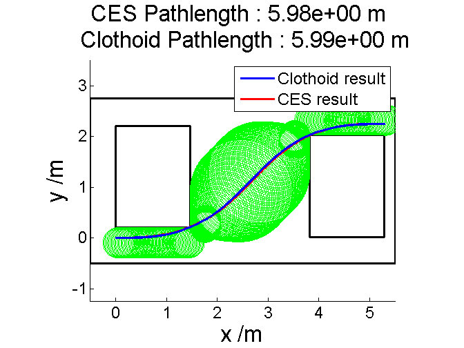
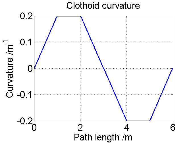
In order to study in isolation the behavior of the Elastic Stretching algorithm, which is one of the main contributions of this paper, we compare our result with a trajectory consisting of clothoid splines. We note that the objective in the shape optimization step is not simply minimum length (which, for a unicycle model, produces paths consisting only of segments with maximum or zero curvature [33]), but instead encodes a notion of minimum overall curvature more compatible with dynamic considerations and speed optimization. To simplify the problem for finding a optimal solution with clothoid splines, we assume a constant vehicle speed along the trajectory. Fig. 10(a) illustrates a scenario of a simple Moose test (S shape turn). Here we consider a turning radius lower bound of $5m$, and an upper bound on the path curvature rate of change of $1m^{-1}s^{-1}$. Fig. 10(b) shows the piecewise linear curvature profile for the clothoid trajectory. The results of the Elastic Stretching approach and the clothoid trajectory are very close in this illustrative example, with an error of $0.17\%$ on the total path length.

IV-E Discussion

Overall, the above numerical experiments show three major trends. First, the smoothed trajectory often results in a noticeable length and traversal time reduction and, in general, a sequence of waypoints that may be easier to track for a lower-level controller. Second, the CES algorithm appears robust with respect to the model used to generate the initial reference trajectory. This is a fundamental property, as in practice one would use a motion planner on a simpler model (e.g., unicycle), and then run a smoothing algorithm with a more sophisticated model. Third, computation times are consistently below one second and in general appear compatible with a real-time implementation.

Figure 8: Smoothed trajectory in a rocky terrain with bicycle model (obstacles in work space)

Figure 9: Smoothed trajectory in a rocky terrain with bicycle model (obstacles inflated in configuration space)

	Time [ms]
Global Planner	$357$
Bubble Generation	$93$ (2 iterations)
Shape Optimization	$203$ (2 iterations)
Speed Optimization	$31$ (2 iterations)
Mapping to Half-Car Model	$114$
Total	$798$

TABLE I: Computation times for planning and smoothing with a bicycle model.

(a) Moose test simulation

(b) Curvature profile of the clothoid trajectory

Figure 10: Comparison of CES output and a clothoid trajectory.

V Conclusions

In this paper we presented a novel algorithm, Convex Elastic Smoothing, for trajectory smoothing which alternates between shape and speed optimization. We showed that both optimization problems can be solved via convex programming, which makes CES particularly fast and amenable to a real-time implementation.

This paper leaves numerous important extensions open for further research. First, it is of interest to extend the CES algorithm to other dynamic systems, such as aerial vehicles or spacecraft. Second, we plan to investigate more thoroughly (1) the robustness of the algorithm when the reference trajectory is not collision-free or dynamically-feasible and (2) the “typical” factor of suboptimality for a number of representative scenarios. Third, for shape optimization, this paper considered smoothness as the objective function. It is of interest to consider alternative objectives, which, for example, could reproduce the trajectories performed by race car drivers (such trajectories may involve significant curvature variations). Fourth, in an effort to make the proposed algorithm “trustworthy,” we plan to characterize upper bounds for computation times under suitable assumptions on the obstacle space. Finally, we plan to deploy the CES algorithm on real self-driving cars.

References

- [1] S. M. LaValle, Planning Algorithms. Cambridge University Press, 2006.
- [2] ——, “Motion planning: Wild frontiers,” IEEE Robotics Automation Magazine, vol. 18, no. 2, pp. 108–118, 2011.
- [3] L. E. Kavraki, P. Švestka, J. C. Latombe, and M. H. Overmars, “Probabilistic roadmaps for path planning in high-dimensional spaces,” IEEE Transactions on Robotics and Automation, vol. 12, no. 4, pp. 566–580, 1996.
- [4] S. M. LaValle and J. J. Kuffner, “Randomized kinodynamic planning,” International Journal of Robotics Research, vol. 20, no. 5, pp. 378–400, 2001.
- [5] J. Pan, L. Zhang, and D. Manocha, “Collision-free and curvature-continuous path smoothing in cluttered environments,” Robotics: Science and Systems, vol. 17, p. 233, 2012.
- [6] D. Hsu, “Randomized single-query motion planning in expansive spaces,” Ph.D. dissertation, Stanford University, 2000.
- [7] R. Geraerts and M. H. Overmars, “Creating high-quality paths for motion planning,” International Journal of Robotics Research, vol. 26, no. 8, pp. 845–863, 2007.
- [8] S. Karaman and E. Frazzoli, “Optimal kinodynamic motion planning using incremental sampling-based methods,” in Proc. IEEE Conf. on Decision and Control, 2010, pp. 7681–7687.
- [9] A. Perez, R. Platt, G. Konidaris, L. Kaelbling, and T. Lozano-Perez, “LQR-RRT*: Optimal sampling-based motion planning with automatically derived extension heuristics,” in Proc. IEEE Conf. on Robotics and Automation, 2012, pp. 2537–2542.
- [10] G. Goretkin, A. Perez, R. Platt Jr., and G. Konidaris, “Optimal sampling-based planning for linear-quadratic kinodynamic systems,” in Proc. IEEE Conf. on Robotics and Automation, 2013, pp. 2429–2436.
- [11] S. Karaman and E. Frazzoli, “Sampling-based optimal motion planning for non-holonomic dynamical systems,” in Proc. IEEE Conf. on Robotics and Automation, 2013, pp. 5041–5047.
- [12] D. J. Webb and J. van den Berg, “Kinodynamic RRT*: Optimal motion planning for systems with linear differential constraints,” in Proc. IEEE Conf. on Robotics and Automation, 2013, pp. 5054–5061.
- [13] P. Jacobs and J. Canny, “Planning smooth paths for mobile robots,” in Nonholonomic Motion Planning. Springer, 1993, pp. 271–342.
- [14] S. Fleury, P. Soueres, J.-P. Laumond, and R. Chatila, “Primitives for smoothing mobile robot trajectories,” IEEE Transactions on Robotics and Automation, vol. 11, no. 3, pp. 441–448, Jun 1995.
- [15] K. Yang and S. Sukkarieh, “An analytical continuous-curvature path-smoothing algorithm,” IEEE Transactions on Robotics, vol. 26, no. 3, pp. 561–568, June 2010.
- [16] S. Lin and X. Huang, Eds., Smooth Path Algorithm Based on A* in Games, ser. Communications in Computer and Information Science. Springer, 2011, vol. 214, pp. 1–34.
- [17] F. Lamiraux and J.-P. Lammond, “Smooth motion planning for car-like vehicles,” IEEE Transactions on Robotics and Automation, vol. 17, no. 4, pp. 498–501, Aug 2001.
- [18] S. Thrun, M. Montemerlo, H. Dahlkamp, D. Stavens, A. Aron, J. Diebel, P. Fong, J. Gale, M. Halpenny, G. Hoffmann, K. Lau, C. Oakley, M. Palatucci, V. Pratt, P. Stang, S. Strohband, C. Dupont, L.-E. Jendrossek, C. Koelen, C. Markey, C. Rummel, J. van Niekerk, E. Jensen, P. Alessandrini, G. Bradski, B. Davies, S. Ettinger, A. Kaehler, A. Nefian, and P. Mahoney, “Stanley: The robot that won the DARPA Grand Challenge,” Journal of Robotic Systems, vol. 23, no. 9, pp. 661–692, 2006.
- [19] C. Urmson et al., “Tartan racing: A multi-modal approach to the darpa urban challenge,” Robotics Institute, http://archive.darpa.mil/grandchallenge/, Tech. Rep. CMU-RI-TR-, April 2007.
- [20] N. Ratliff, J. A. Zucker, M.and Bagnell, and S. Srinivasa, “Chomp: Gradient optimization techniques for efficient motion planning,” in Proc. IEEE Conf. on Robotics and Automation, 2009, pp. 489–494.
- [21] J. Biggs and W. Holderbaum, “Planning rigid body motions using elastic curves,” Mathematics of Control, Signals, and Systems, vol. 20, no. 4, pp. 351–367, 2008.
- [22] O. Brock and O. Khatib, “Elastic strips: A framework for motion generation in human environments,” International Journal of Robotics Research, vol. 21, no. 12, pp. 1031–1052, 2002.
- [23] S. Quinlan and O. Khatib, “Elastic bands: Connecting path planning and control,” in Proc. IEEE Conf. on Robotics and Automation, vol. 2, Atlanta, GA, May 1993, pp. 802–807.
- [24] S. Boyd and L. Vandenberghe, Convex Optimization. Cambridge University Press, 2004.
- [25] S. Erlien, S. Fujita, and J. C. Gerdes, “Safe driving envelopes for shared control of ground vehicles,” in Advances in Automotive Control, vol. 7, no. 1, 2013, pp. 831–836.
- [26] T. Lipp and S. Boyd, “Minimum-time speed optimisation over a fixed path,” International Journal of Control, vol. 87, no. 6, pp. 1297–1311, 2014.
- [27] E. Schmerling, L. Janson, and M. Pavone, “Optimal sampling-based motion planning under differential constraints: the driftless case,” in Proc. IEEE Conf. on Robotics and Automation, 2015, pp. 2368–2375.
- [28] L. Janson, E. Schmerling, A. Clark, and M. Pavone, “Fast marching tree: A fast marching sampling-based method for optimal motion planning in many dimensions,” International Journal of Robotics Research, vol. 34, no. 7, pp. 883–921, 2015.
- [29] D. Milliken, Race Car Vehicle Dynamics: Problems, Answers, and Experiments. SAE International, 2003.
- [30] A. D. and J. Jerez, “Forces professional,” embotech GmbH (http://embotech.com/FORCES-Pro), Jul. 2014.
- [31] J. Hwan Jeon, R. V. Cowlagi, S. C. Peters, S. Karaman, E. Frazzoli, P. Tsiotras, and K. Iagnemma, “Optimal motion planning with the half-car dynamical model for autonomous high-speed driving,” in American Control Conference, 2013, pp. 188–193.
- [32] J. Ackermann, “Robust decoupling, ideal steering dynamics and yaw stabilization of 4WS cars,” Automatica, vol. 30, no. 11, pp. 1761–1768, 1994.
- [33] L. E. Dubins, “On curves of minimal length with a constraint on average curvature and with prescribed initial and terminal positions and tangents,” American Journal of Mathematics, vol. 79, pp. 497–516, 1957.