Towards the statistical detection of the warm-hot intergalactic medium in inter-cluster filaments of the cosmic web

Abstract

Modern analyses of structure formation predict a universe tangled in a ‘cosmic web’ of dark matter and diffuse baryons. These theories further predict that at low-$z$, a significant fraction of the baryons will be shock-heated to $T\sim 10^{5}-10^{7}$ K yielding a warm-hot intergalactic medium (WHIM), but whose actual existence has eluded a firm observational confirmation. We present a novel experiment to detect the WHIM, by targeting the putative filaments connecting galaxy clusters. We use HST/COS to observe a remarkable QSO sightline that passes within $\Delta d=3$ Mpc from the $7$ inter-cluster axes connecting $7$ independent cluster-pairs at redshifts $0.1\leq z\leq 0.5$. We find tentative excesses of total H i, narrow H i (NLA; Doppler parameters $b<50$), broad H i (BLA; $b\geq 50$) and O vi absorption lines within rest-frame velocities of $\Delta v\lesssim 1000$from the cluster-pairs redshifts, corresponding to $\sim 2$, $\sim 1.7$, $\sim 6$ and $\sim 4$ times their field expectations, respectively. Although the excess of O vi likely comes from gas close to individual galaxies, we conclude that most of the excesses of NLAs and BLAs are truly intergalactic. We find the covering fractions, $f_{c}$, of BLAs close to cluster-pairs are $\sim 4-7$ times higher than the random expectation (at the $\sim 2\sigma$ c.l.), whereas the $f_{c}$ of NLAs and O vi are not significantly enhanced. We argue that a larger relative excess of BLAs compared to those of NLAs close to cluster-pairs may be a signature of the WHIM in inter-cluster filaments. By extending the present analysis to tens of sightlines our experiment offers a promising route to detect the WHIM.

1 Introduction

Perhaps the most distinctive feature of the cosmic web is its intricate pattern of filamentary structures. Cosmological simulations in a $\Lambda$ cold dark matter ($\Lambda$CDM) paradigm predict that these filaments account for $\sim 40\%$ of all mass in the Universe at $z=0$ and occupy roughly $\sim 10\%$ of the volume (e.g. Aragón-Calvo et al., 2010). When gas and hydrodynamical effects are included in these simulations, a remarkable conclusion is reached: $\sim 30-50\%$ of baryons at low-$z$ should reside in dense filaments, primarily in the form of a diffuse gas phase with temperatures $T\sim 10^{5}-10^{7}$ K, which would be very difficult to detect (e.g. Cen & Ostriker, 1999; Davé et al., 2001). This material is usually referred to as the WHIM, and indeed is currently the best candidate to host a significant fraction of the so-called ‘missing baryons’ at $z<1$ (Persic & Salucci, 1992; Fukugita et al., 1998; Bregman, 2007; Prochaska & Tumlinson, 2009; Shull et al., 2012, and references therein). According to these models, the physical origin of the WHIM is through gravitational shocks from the collapse of matter into the large scale structure (LSS) of the Universe.

One well-studied example of gravitational shock-heating is the so-called intracluster medium (ICM) of galaxy clusters, where the virial temperatures typically reach $T\sim 10^{7}-10^{8}$ K. A plasma at these temperatures mostly cools through Bremsstrahlung (a.k.a. free-free) thermal radiation, emitting $X$-rays at $\sim$ keV energies that may be observed with modern satellites (e.g. Kravtsov & Borgani, 2012, and references therein). $X$-ray spectroscopy has also revealed the presence of high-ionization state metal emission lines in the ICM, consistent with these large temperatures (e.g. Sanders et al., 2008). Thereby one constrains the density, chemical abundances and morphology of the ICM. Several decades of research have revealed a highly enriched medium ($\sim\frac{1}{3}$ solar) with a total mass consistent with the cosmic ratio of baryons to dark matter (e.g. Allen et al., 2008).

In the $\Lambda$CDM paradigm, galaxy clusters correspond to the nodes of the cosmic web, i.e., they mark the intersection of several filamentary threads. These models further predict that matter flows through the filamentary structures, driving the growth of the galaxy clusters. Ideally, one would image these filaments in a similar manner to the ICM to reveal their structure and physical properties as tests of the cosmic web paradigm. Unfortunately, once at the outskirts of galaxy clusters, the densities and temperatures are too low for viable $X$-ray detection in emission (e.g. Bremsstrahlung radiation is proportional to the density squared of the emitting gas). To study this dominant component of the cosmic web and its putative relationship to a WHIM, one must pursue alternate strategies.

In principle, one may scour the volumes surrounding galaxy clusters for signatures of cosmic filaments. A random search, however, would be compromised by the fact that their volume filling factor is predicted to be low, even in this environment. To raise the probability of isolating a cosmic filament, researchers have turned to pairs of neighbouring clusters on the expectation that these massive structures will be preferentially connected. Indeed, cosmological dark matter simulations find high probabilities of having a coherent filamentary structure between close ($<20$ Mpc) and massive ($>10^{14}$ M_☉) galaxy clusters (e.g. Colberg et al., 2005; González & Padilla, 2010; Aragón-Calvo et al., 2010). This probability is mostly a function of the galaxy cluster masses and the separation between them: the larger the masses and the shorter the separation, the higher the probability. Therefore, the volume between close pairs of galaxy clusters is a natural place to search for signatures of filaments and an associated WHIM.

Inter-cluster filaments (i.e. filaments between galaxy cluster pairs) have been inferred from galaxy distributions, either individually from spectroscopic galaxy surveys (e.g. Pimbblet et al., 2004), or by stacking analysis from photometric galaxy surveys (e.g. Zhang et al., 2013). While these studies confirm the strategy to focus on cluster pairs, they provide limited information into the nature of cosmic filaments; these luminous systems represent $\lesssim 10\%$ of the baryonic matter, their distribution and motions need not trace the majority of the gas, and they offer no insight into the presence of a WHIM.

Table 1: Properties of the observed QSO Q1410.

QSO Name	R.A.	Dec.	$z_{\rm QSO}$	Magnitudes
	(hr min sec)	(deg min sec)		$r$	NUV	FUV
(1)	(2)	(3)	(4)	(5)	(6)	(7)
SDSS J141038.39+230447.1	14 10 38.39	$+$23 04 47.18	0.7958	17.0	17.4	18.7

(1) Name of the QSO. (2) Right ascension (J2000). (3) Declination (J2000). (4) Redshift of the QSO. (5) Apparent $r$ (visual) magnitude from Sloan Digital Sky Survey (SDSS). (6) Apparent near- ultra-violet (UV) magnitude from GALEX. (7) Apparent far-UV magnitude from GALEX.

Promising results from stacking multiple inter-cluster regions have found an excess of $X$-ray counts in such regions with respect to the background (Fraser-McKelvie et al., 2011). In contrast to galaxies, one would be truly observing the bulk of baryonic matter. Unfortunately, the geometry of the emission and the actual origin of the detected photons was not well constrained by this original work. Remarkable detection of individual inter-cluster filaments have also been reported from gravitational weak lensing signal (Dietrich et al., 2012), and $X$-ray emission (Kull & Böhringer, 1999; Werner et al., 2008). Despite their indisputable potential for characterizing cosmological filaments, these techniques are currently limited to the most massive systems with geometries maximizing the observed surface densities, i.e. filaments almost aligned with the line-of-sight (LOS).

To complement these and other relevant studies to address the ‘missing baryons’ problem (e.g. Nevalainen et al., 2015; Planck Collaboration et al., 2015; Hernández-Monteagudo et al., 2015), we have designed a program to detect the putative filaments connecting cluster pairs in absorption. This technique has several advantages over attempts to detect the gas in emission. First, absorption-line spectroscopy is linearly proportional to the density of the absorbing gas, offering much greater sensitivity to a diffuse medium. Second, the absorption lines encode the kinematic characteristics of the gas, including constraints on the temperature, turbulence, and LOS velocity. Third, one may assess the chemical enrichment and ionization state of the gas through the analysis of multiple ions. The obvious drawback to this technique is that one requires the fortuitous alignment of a bright background source with these rare cluster pairs, to probe a greatly reduced spatial volume: in essence a single pinprick through a given filament. However, with a large enough survey one may also statistically map the geometry/morphology of the filaments.

Here we focus on far ultra-violet (FUV) spectroscopy leveraging the unprecedented sensitivity of the Cosmic Origins Spectrograph (COS) onboard the Hubble Space Telescope (HST), to greatly increase the sample of inter-cluster filaments probed. With such UV capabilities we can directly access H i —the strongest and most common transition for probing the intergalactic medium (IGM). Having direct coverage of H i independent of the presence of metals is of great value for detecting the WHIM (e.g. Richter et al., 2006; Danforth et al., 2010), because this medium may remain metal poor. Neutral hydrogen generally traces cool and photoionized gas, but it may also trace collisionally ionized gas in the WHIM through broad (Doppler parameters $b\gtrsim 50$) lines (e.g. Tepper-García et al., 2012). Although the circumgalactic medium (CGM) surrounding galaxies is responsible for producing H i absorption lines (especially at column densities $\gtrsim 10^{15}$ cm^-2; e.g. Tumlinson et al., 2013), the majority of them must arise in the diffuse IGM (e.g. Prochaska et al., 2011; Tejos et al., 2012, 2014). FUV spectroscopy also allows the detection of the O vi doublet, a common highly ionized species. The physical origin of O vi absorption lines is controversial, including scenarios of photoionized and/or collisionally ionized gas in the CGM of individual galaxies and/or galaxy groups (e.g. Tripp et al., 2008; Thom & Chen, 2008; Wakker & Savage, 2009; Stocke et al., 2014; Savage et al., 2014). Thus, a collisionally ionized component could well be present, some of which may come from a WHIM (although see Oppenheimer & Davé, 2009; Tepper-García et al., 2011).

In a more general context, H i and O vi offer an optimal approach to study filamentary gas in absorption. As mentioned, this pair of diagnostics correspond to the most common transitions observed in the low-$z$ Universe (e.g. Danforth & Shull, 2008; Tripp et al., 2008; Danforth et al., 2014), allowing a good characterization of the background signal against which one may search for signatures of WHIM in filamentary gas. Such signatures could include an elevated/suppressed incidence, covering fractions, and/or unique distributions in the strengths or widths of the absorption features. In contrast to studies where absorption systems could be associated with filaments on an individual basis (e.g. Aracil et al., 2006; Narayanan et al., 2010), our methodology is statistical in nature and a large sample of independent structures must be collected.

The current advent of big extragalactic surveys makes our approach feasible. For instance, the SDSS (Ahn et al., 2014) provides large samples of LSS traced by galaxies and known QSOs in the same volume. In particular, by using the galaxy cluster catalog of Rykoff et al. (2014) we have constructed a cluster-pair sample and found that, on average, a random sightline extending between $0.1\leq z\leq 0.5$ intersects $1\pm 1$ independent cluster-pairs with projected separations of $\leq 3$ Mpc to the inter-cluster axis (defined as the line segment joining the centers of the two galaxy clusters of a pair; see Figure 1 for an illustration, and Section 3 for further details), with a very skewed distribution towards zero (see Section 3.4). In order to enhance the efficiency however, we have cross-matched such cluster-pair sample with known FUV luminous QSOs from the Schneider et al. (2010) catalog, and identified particular sightlines intersecting more than one of these structures. Our approach is highly complementary to that of Wakker et al. (2015), where a single galaxy filament is targeted with multiple QSO sightlines.

In this paper we present HST/COS FUV observations of a single bright QSO at $z\approx 0.8$ (namely SDSS J$141038.39$+$230447.1$, hereafter referred to as Q1410; see Table 1), whose unique sightline intersects $7$ independent cluster-pairs within $3$ Mpc from their inter-cluster axes. This sightline is highly exceptional; the random expectation of finding such a number of cluster-pairs is $\lesssim 0.01\%$ (see Section 3.4). With this one dataset, we offer a first statistical assessment of the presence of diffuse gas close to cluster-pairs. Although we are only reporting tentative results ($\sim 1-2\sigma$ c.l.), the primary focus of this manuscript is to establish the experimental design and methodology. Future work will extend the present study to tens of sightlines, eventually leading towards the statistical detection of the WHIM in inter-cluster filaments of the cosmic web.

Our paper is structured as follows. In Section 2 we present both the galaxy cluster catalog used to create our cluster-pair sample and our HST/COS observations of Q1410. In Section 3 we characterize the volume around the Q1410 sightline in terms of known clusters and cluster-pairs, quantifying how unusual the Q1410 field is. In Section 4 we provide a full characterization of the Q1410 HST/COS FUV spectrum in terms of absorption line systems, regardless of the presence of known intervening structures. In Section 5 we present our methodology to cross-match the information provided by the cluster-pair sample and absorption line systems, while in Section 6 we present our observational results for the Q1410 field. A discussion of these results is presented in Section 7, and a summary of the paper is presented in Section 8. Supplementary material is presented in the Appendix. All distances are in co-moving coordinates assuming $H_{0}=67.3$Mpc^-1, $\Omega_{\rm m}=0.315$, $\Omega_{\rm\Lambda}=0.685$, $k=0$ (unless otherwise stated), where $H_{0}$, $\Omega_{\rm m}$, $\Omega_{\rm\Lambda}$ and $k$ are the Hubble constant, mass energy density, ‘dark energy’ density and spatial curvature, respectively (Planck Collaboration et al., 2014).

2 Data

2.1 Galaxy clusters

In this section we briefly describe the cluster catalog used in the present paper. We used red-sequence Matched-filter Probabilistic Percolation (redMaPPer) (Rykoff et al., 2014) applied to the SDSS Eighth Data Release (DR8) (Aihara et al., 2011). This is one of the largest galaxy cluster catalogs currently available, containing $\sim 25\,000$ rich galaxy clusters ($>20$ galaxies having luminosities $L\geq 0.2L^{*}$) at $0.08\leq z\leq 0.55$.

The redMaPPer catalog is very well suited for statistical analysis: it defines clusters properties in terms of probabilities (e.g. position, richness, redshift, galaxy members), with a well understood selection function; it adopts an optimal mass-richness relationship (Rykoff et al., 2012); and it has high completeness and purity levels compared to others cluster catalogs (Rykoff et al., 2014; Rozo & Rykoff, 2014; Rozo et al., 2014).

In this paper we used an extension of the published redMaPPer catalog, including galaxy clusters with richness below $20$ but larger than $10$. The mass–richness relation relevant to the redMaPPer catalog is,

$$\ln\left(\frac{M_{200}}{h^{-1}_{70}\,10^{14}M_{\odot}}\right)=1.72+1.08\ln\left(\frac{\lambda}{60}\right)\ \rm{,}$$ (1)

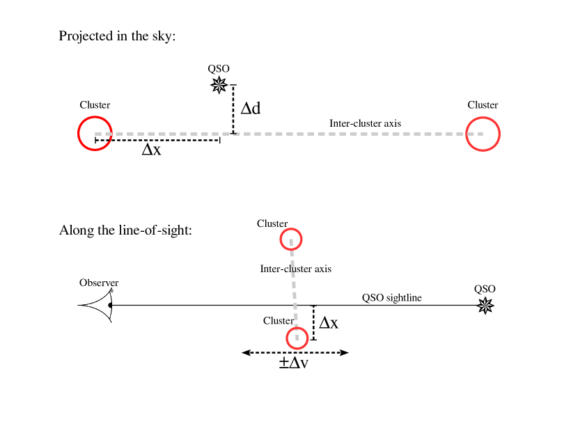
Figure 1: Schematic representation of our survey geometry projected in the sky (top) and along the line-of-sight (bottom), for a single cluster-pair. Galaxy clusters are represented by red circles, while the inter-cluster axis is represented by the grey dashed lines. The QSO itself is represented by a eight-pointed star. The impact parameter between the QSO sightline and the inter-cluster axis is defined as $\Delta d$, while the distance to the closest cluster of the pair along the projected inter-cluster axis is defined as $\Delta x$. A rest-frame velocity window around the position of the cluster-pair is defined as $\pm\Delta v$.

with a typical scatter of $\sim 0.25$ in $\ln(M)$ (Rykoff et al., 2012), where $M_{200}$ is the total mass enclosed within an overdensity of $200$ times the critical density of the Universe,$\rho_{\rm crit}$; $h_{70}$ is the dimensionless Hubble parameter $h_{70}\equiv H_{0}/(70$  km s^-1 Mpc${}^{-1})$; $M_{\odot}$ is the mass of the sun; and $\lambda$ is the richness of galaxies with luminosities $L\geq 0.2L^{*}$ (corrected for incompleteness). Extrapolating this relation to $\lambda=10$ we get a minimum mass $M_{200}(\lambda=10)\approx 0.8\times 10^{14}M_{\odot}$ in our assumed cosmology (see end of Section 1). Therefore, our adopted limit should still ensure a reasonable large minimum mass limit. We also computed an estimate of the virial radius, $R_{200}$, simply defined as the radius at which the $M_{200}$ is enclosed,

$$R_{200}\equiv\left(\frac{M_{200}}{\frac{4}{3}\pi 200\rho_{\rm crit}}\right)^{1/3}\ \rm{.}$$ (2)

We note that because we are only using these clusters as tracers of high density regions in the cosmic web, the exact mass of the clusters will not be particularly relevant, making potential systematic uncertainties in the mass-richness calibration and its extrapolation to lower values not a critical issue. Moreover, low richness cluster samples suffer more from impurity and incompleteness (Rykoff et al., 2014), but such issues should not create a fake signal in differentiating the properties of absorption line systems in environments traced by these cluster-pairs with respect to the field, in the presence of real inter-cluster filaments. On the contrary, our approach is conservative in the sense that impurity and incompleteness would dilute such a signal, if present.

For the purposes of this paper, we also required the clusters to lie between $0.1\leq z\leq 0.5$, yielding a total of $162\,144$ clusters (see Section 3.1 and Appendix A for further details).

Although the redMaPPer catalog is mostly based on photometry, the spectroscopic redshift of the most likely centre is also given when available (typically from its brightest cluster galaxy (BCG)). This is advantageous for our experiment; a high precision in the cluster redshifts is needed for a reliable association with the gas observed in absorption with inter-cluster filaments (if any). About $44\%$ ($71\,701/162\,144$) of the redMaPPer clusters have spectroscopic redshifts, yielding velocity precision of $\approx 30$ in those clusters’ rest frames. We note that for the subsample of clusters most relevant to our paper (i.e. within $20$ Mpc of the Q1410), such fraction increases to $\sim 70\%$ ($40/57$; see Section 3.1 for further details).

2.2 Q1410 absorption lines

2.2.1 Specific selection of Q1410

In this section we describe in detail the selection criteria of our targeted QSO, Q1410. We emphasize that the original selection of Q1410 was done using the galaxy cluster catalog published by Hao et al. (2010) instead of the redMaPPer catalog (Rykoff et al., 2014) used here.

The Gaussian Mixture Brightest Cluster Galaxy (GMBCG) catalog (Hao et al., 2010) is based on data from the Seventh Data Release (DR7) of the SDSS (Abazajian et al., 2009), and similar to redMaPPer, it is mainly based on photometry. From the GMBCG catalog we searched for cluster-pairs where at least one member has a spectroscopic redshift and where the redshift difference between them is less than $3\times$ the combined redshift uncertainty, and over clusters having GMBCG richness $>15$. We then measured the transverse co-moving separation between clusters at the redshift of the cluster with spectroscopic identification (if both clusters had spectroscopic redshifts we used the average redshift), and kept the ones separated by $<25$ Mpc.

Table 2: Properties of the redMaPPer clusters at $0.1\leq z\leq 0.5$ and within $20$ Mpc from the Q1410 sightline.

Cluster ID	R.A.	Dec.	$z_{\rm spec}$	$z_{\rm photo}$	Richness	Mass	$R_{200}$	Impact parameter
	(degrees)	(degrees)				($10^{14}\ M_{\sun}$)	( Mpc)	(degrees)	(Mpc)	($R_{200}$)
(1)	(2)	(3)	(4)	(5)	(6)	(7)	(8)	(9)	(10)	(11)
1	212.994666	21.418861	0.1335	0.150 $\pm$ 0.006	11.0	0.92	0.9	1.6895	16.9	18.5
2	213.481691	22.808351	0.1376	0.147 $\pm$ 0.005	20.4	1.80	1.1	0.8039	8.3	7.3
3	214.114059	23.256258	0.1381	0.138 $\pm$ 0.005	33.0	3.03	1.4	1.3484	13.9	10.3
4	213.817562	24.020988	0.1386	0.152 $\pm$ 0.006	16.5	1.43	1.1	1.4184	14.7	13.9
5	213.014763	22.125043	0.1413	0.141 $\pm$ 0.006	18.3	1.60	1.1	1.0093	10.6	9.7
6	213.223623	22.319874	0.1417	0.150 $\pm$ 0.005	20.3	1.79	1.1	0.9208	9.7	8.6
7	213.330826	22.510559	…	0.143 $\pm$ 0.005	17.9	1.56	1.1	0.8405	9.0	8.3
8	213.664909	22.216942	0.1535	0.171 $\pm$ 0.007	10.9	0.91	0.9	1.2667	14.5	16.0
9	212.712357	23.086999	0.1580	0.157 $\pm$ 0.006	13.0	1.11	1.0	0.0487	0.6	0.6
10	212.162442	21.946327	0.1596	0.145 $\pm$ 0.006	11.3	0.95	0.9	1.2231	14.5	15.9
11	212.999309	24.435343	0.1612	0.171 $\pm$ 0.006	16.1	1.39	1.0	1.3907	16.6	16.1
12	212.674015	22.495683	0.1733	0.179 $\pm$ 0.006	23.0	2.05	1.2	0.5842	7.5	6.4
13	212.895979	23.605206	0.1787	0.167 $\pm$ 0.007	11.4	0.96	0.9	0.5684	7.5	8.3
14	213.557346	22.914918	0.1918	0.195 $\pm$ 0.007	12.4	1.05	0.9	0.8423	11.9	12.8
15	212.123899	22.560692	0.2220	0.241 $\pm$ 0.012	11.2	0.94	0.9	0.7167	11.6	13.1
16	211.805856	23.845513	0.2359	0.233 $\pm$ 0.008	21.4	1.90	1.1	1.0955	18.8	16.8
17	213.277561	24.079481	0.2392	0.234 $\pm$ 0.012	10.6	0.89	0.9	1.1488	20.0	23.1
18	213.029395	23.923686	0.2424	0.254 $\pm$ 0.010	24.9	2.23	1.2	0.9094	16.0	13.6
19	212.319446	22.314272	0.2914	0.482 $\pm$ 0.021	11.4	0.96	0.9	0.8275	17.3	19.8
20	212.415280	22.627699	0.3127	0.306 $\pm$ 0.020	11.4	0.96	0.9	0.5052	11.3	13.0
21	213.395595	23.114057	…	0.327 $\pm$ 0.020	12.2	1.03	0.9	0.6775	15.8	17.9
22	212.831535	22.621344	0.3382	0.368 $\pm$ 0.017	30.0	2.73	1.2	0.4849	11.6	9.6
23	212.723980	22.929555	0.3412	0.357 $\pm$ 0.017	28.1	2.54	1.2	0.1614	3.9	3.3
24	213.000928	22.437411	…	0.345 $\pm$ 0.018	23.6	2.10	1.1	0.7152	17.5	15.7
25	212.293470	23.265859	0.3465	0.349 $\pm$ 0.019	21.2	1.88	1.1	0.3849	9.4	8.8
26	212.684410	23.402739	0.3506	0.358 $\pm$ 0.024	11.4	0.96	0.9	0.3237	8.0	9.4
27	212.770942	23.232412	0.3508	0.357 $\pm$ 0.022	10.4	0.87	0.8	0.1836	4.6	5.5
28	213.066601	23.075991	0.3511	0.378 $\pm$ 0.021	20.6	1.82	1.1	0.3741	9.3	8.8
29	212.600828	23.822434	0.3520	0.358 $\pm$ 0.020	15.0	1.29	0.9	0.7446	18.5	19.7
30	212.854438	22.531418	…	0.365 $\pm$ 0.021	13.5	1.15	0.9	0.5769	14.8	16.5
31	212.861147	22.341353	0.3718	0.385 $\pm$ 0.016	22.8	2.03	1.1	0.7614	19.9	18.3
32	213.011303	23.110255	0.3722	0.395 $\pm$ 0.019	13.6	1.16	0.9	0.3246	8.5	9.4
33	212.737954	23.677308	0.3725	0.379 $\pm$ 0.017	18.4	1.61	1.0	0.6018	15.8	15.7
34	213.115594	22.812719	0.3725	0.400 $\pm$ 0.022	16.9	1.46	1.0	0.4973	13.0	13.4
35	212.604626	23.277634	…	0.376 $\pm$ 0.018	22.2	1.98	1.1	0.2043	5.4	5.0
36	212.538462	23.376505	…	0.384 $\pm$ 0.019	17.6	1.53	1.0	0.3170	8.5	8.7
37	212.800638	23.052477	0.4138	0.426 $\pm$ 0.015	20.0	1.76	1.0	0.1323	3.8	3.7
38	212.609281	22.997888	0.4159	0.425 $\pm$ 0.015	10.6	0.89	0.8	0.0942	2.7	3.4
39	212.177450	22.994366	0.4188	0.424 $\pm$ 0.015	25.4	2.28	1.1	0.4522	13.1	11.9
40	213.120494	22.548543	…	0.420 $\pm$ 0.014	38.4	3.57	1.3	0.6800	19.8	15.4
41	211.935365	23.227769	0.4199	0.416 $\pm$ 0.019	10.7	0.90	0.8	0.6825	19.9	24.5
42	212.374306	22.818205	…	0.420 $\pm$ 0.019	17.3	1.50	1.0	0.3710	10.8	11.2
43	212.420269	23.093511	…	0.428 $\pm$ 0.018	14.5	1.24	0.9	0.2209	6.6	7.3
44	212.593164	22.699892	…	0.430 $\pm$ 0.017	12.1	1.02	0.8	0.3848	11.5	13.6
45	211.957129	23.106715	…	0.434 $\pm$ 0.014	28.6	2.59	1.1	0.6471	19.4	16.9
46	212.999005	22.821469	0.4358	0.443 $\pm$ 0.019	12.5	1.06	0.9	0.4052	12.2	14.3
47	212.607221	22.800250	…	0.440 $\pm$ 0.018	13.0	1.10	0.9	0.2837	8.6	10.0
48	212.115194	23.041513	0.4397	0.442 $\pm$ 0.016	11.1	0.94	0.8	0.5027	15.3	18.7
49	212.968630	22.717594	…	0.441 $\pm$ 0.021	11.0	0.92	0.8	0.4604	14.0	17.3
50	212.980494	22.615241	…	0.441 $\pm$ 0.018	15.6	1.34	0.9	0.5505	16.7	18.2
51	212.172529	23.471857	…	0.445 $\pm$ 0.018	15.6	1.35	0.9	0.5952	18.3	19.8
52	212.710891	23.162554	…	0.452 $\pm$ 0.017	11.4	0.96	0.8	0.0951	3.0	3.6
53	212.336805	22.647284	…	0.454 $\pm$ 0.019	15.5	1.34	0.9	0.5251	16.4	18.0
54	212.658634	23.039911	0.4582	0.437 $\pm$ 0.014	37.2	3.44	1.3	0.0399	1.3	1.0
55	212.346270	23.242090	0.4585	0.449 $\pm$ 0.016	15.6	1.35	0.9	0.3310	10.4	11.4
56	213.213654	22.988852	0.4603	0.477 $\pm$ 0.013	47.9	4.52	1.4	0.5176	16.4	11.9
57	213.210168	23.112030	0.4615	0.469 $\pm$ 0.013	48.9	4.62	1.4	0.5071	16.1	11.7

(1) Cluster ID. (2) Right ascension (J2000). (3) Declination (J2000). (4) Spectroscopic redshift. (5) Photometric redshift. (6) Richness of galaxies having $L\geq 0.2L^{*}$, corrected for incompleteness (hence non-integer). (7) Inferred mass using Equation 1; typical scatter of $\sim 0.25$ in $\ln(M)$ (Rykoff et al., 2012). (8) Inferred virial radii of the cluster using Equation 2. (9) Projected separation to the Q1410 sightline in degrees. (10) Projected separation to the Q1410 sightline in  Mpc. (11) Projected separation to the Q1410 sightline in units of our $R_{200}$ estimation.

We selected our target from the QSO catalog published by Schneider et al. (2010), which is also based on SDSS DR7 data. This catalog comprises $\gtrsim 100\,000$ QSOs with well known magnitudes and spectroscopic redshifts. We looked for QSOs having redshifts greater than individual cluster-pairs and located inside their sky-projected cylinder areas as defined above. We imposed a magnitude limit of $r<17.5$ mag to select relatively bright QSOs. We gave priority to QSOs $z>0.3$, ensuring large redshift path coverage. We also searched in the Galaxy Evolution Explorer (GALEX) (Martin et al., 2005) database and prioritized those QSOs with high FUV fluxes to ensure no higher-$z$ Lyman Limit Systems (LLS) were present, enabling a signal-to-noise ratio (S/N) $S/N\sim 10$ spectra to be observed in a relatively short exposure time (no larger than $15$ orbits). For each of these QSOs we counted the number of independent cluster-pairs (defined as those which were separated by more than $1000$ km s^-1 from another, and by more than $5000$ km s^-1 from the background QSO in rest-frame velocity space) at impact parameters $\Delta d\leq 2$ Mpc from the QSO sightline (see Figure 1 for an illustration). We note that in this paper we adopted a larger limit of $3$ Mpc as the fiducial minimum impact parameter (see Section 3), motivated by the results obtained in Section 6. We finally selected the sightline that maximized the number of independent cluster-pair structures, for the mininum observing time. Table 1 presents a summary of the properties of the targeted QSO, Q1410.

2.2.2 HST/COS observations and data reduction of Q1410

In this paper we present FUV spectroscopic data of Q1410 (see Table 1 for a summary of its main properties) from HST/COS (Green et al., 2012) taken under program General Observer (GO) 12958 (PI Tejos).

The QSO Q1410 was observed in August 2013 using both G130M and G160M gratings centred at $1318$ and $1611$ Å respectively, using the four fixed-pattern noise positions available for each configuration. These settings provided medium-resolution ($R\equiv\frac{\lambda}{\Delta\lambda}\sim 16\,000-21\,000$ or $FWHM\sim 0.07-0.09$Å) over the FUV wavelength range of $\sim 1160-1790$ Å, but having two $\sim 20$ Å gaps around each central wavelength. We chose this approach rather than a continuous wavelength coverage to increase the S/N at spectral regions where we expected to find H i absorption line systems associated with inter-cluster filaments. Having multiple FP-POS (as in our observations) is crucial, however, to minimize the effect of fixed-pattern noise present in COS (see Osterman et al., 2011; Green et al., 2012, for more details on the technical aspects of COS).

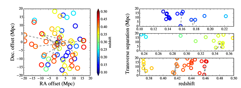
Figure 2: Representation of the LSSs within $20$ Mpc around the Q1410 sightline at redshifts $0.1\leq z\leq 0.5$, as traced by the $57$ galaxy clusters from the redMaPPer catalog (see Section 3 and Table 2). Galaxy clusters are represented by coloured circles according to redshift, as given by the colour bar scale. Cluster-pairs at impact parameters $\Delta d\leq 3$ Mpc of the Q1410 sightline are represented by dashed grey lines. The left panel shows to the projected in the sky distributions in co-moving  Mpc, where the Q1410 sightline is represented by the yellow star at the origin. The right panel shows the distribution along the line-of-sight in terms of total transverse separation (in co-moving  Mpc) as a function of redshift (note that inter-cluster axes appear as hyperbolas in these coordinates). See Section 3 for further details.

Table 3: Clusters-pairs around Q1410.

Pair ID	Cluster IDs	$z$	Separation between clusters		$\Delta d$	$\Delta x$	Both spec-$z$?	Grouped ID
			Transverse (Mpc)	LOS (km s-1)	(Mpc)	(Mpc)
(1)	(2)	(3)	(4)	(5)	(6)	(7)	(8)	(9)
1	9,10	0.1588	14.7	419	0.48	0.31	y	1
2	12,13	0.1760	14.7	1378	1.54	7.33	y	2
3	23,25	0.3439	12.7	1189	1.85	3.43	y	3
4	25,28	0.3488	18.1	1021	2.29	9.00	y	4
5	34,35	0.3726	17.3	771	2.76	4.63	n	5
6	37,42	0.4139	13.2	1365	2.59	2.79	n	6
7	37,38	0.4149	5.3	435	1.86	1.99	y	6
8	37,39	0.4163	16.7	1043	1.16	3.62	y	6
9	37,41	0.4169	23.6	1284	0.03	3.80	y	6
10	54,55	0.4584	11.1	68	1.05	0.69	y	7
11	54,57	0.4599	16.2	682	1.24	0.21	y	7

(1) Cluster-pair ID. (2) IDs of clusters defining the cluster-pair as given in Table 2. (3) Redshift of the cluster-pair. (4) Transverse separation between clusters in  Mpc. (5) Along the line-of-sight separation between the clusters in rest-frame . (6) Impact parameter to the Q1410 sightline. (7) Projected on the sky distance to the closest cluster of the pair, along the inter-cluster axis. (8) Whether both clusters have spectroscopic redshifts. (9) Grouped ID for independent cluster-pairs.

Data reduction was performed in the same fashion as presented in Finn et al. (2014) and Tejos et al. (2014), for the G130M and G160M COS gratings. In summary, we used the calcos v2.18.5 pipeline with extraction windows of $25$ and $20$ pixels for the G130M and G160M gratings, respectively. We applied a customized background estimation smoothing (boxcar) over $1000$ and $500$ pixels for the FUVA and FUVB stripes, respectively, while masking out and linearly interpolating over regions close to geocoronal emission lines and pixels flagged as having bad quality. The uncertainty was calculated in the same manner as in calcos but using our customized background. The co-alignment was performed using strong Galactic interstellar medium (ISM) features as reference. We finally binned the original spectra having dispersions of $\sim 0.010$ and $\sim 0.012$ Å  pixel^-1 for the G130M and G160M gratings respectively, into a single linear wavelength scale of $0.0395$ Å  pixel^-1 (roughly corresponding to two pixels per resolution element). Due to the difficulties in assessing the degree of geocoronal contamination in the final reduced Q1410 spectrum, we opted to mask out the spectral regions close to rest-frame N i, H i  and O i (namely $1300.0-1307.5$, $1198.5-1201.0$ and $1213.5-1217.8$ Å, respectively).

Our pseudo-continuum fit was modelled as in Tejos et al. (2014), but also introducing the presence of three partial LLS breaks at $\approx 1232$, $1401$ and $1637$ Å. Figure 14 shows the reduced Q1410 spectrum (black line), its corresponding uncertainty (green lines) and our adopted pseudo-continuum fit (blue dotted line).

3 Characterization of large-scale structures around the Q1410 sightline

3.1 Galaxy clusters

From the redMaPPer catalog described in Section 2.1, we define a subsample of clusters according to the following criteria:

• the redshift has to lie between $0.1\leq z\leq 0.5$; and,

• the impact parameter to the Q1410 sightline has to be no larger than $20$ Mpc.

There are a total of $57$ clusters from the redMaPPer catalog satisfying the aforementioned criteria, whose relevant information is presented in Table 2. We also show their distribution around the Q1410 sightline in LABEL:{fig:field} (coloured circles).

The redshift range of $0.1\leq z\leq 0.5$ was chosen to ensure simultaneous coverage of both H i and O vi transitions from our COS data, while the impact parameter of $20$ Mpc (arbitrary) was chosen to cover scales expected to be relevant for inter-cluster filaments (e.g. Colberg et al., 2005; González & Padilla, 2010).

In Appendix A we show how our subsample of clusters compares to appropriate control samples drawn from the full redMaPPer catalog. We found no statistically significant differences for the mass (richness) and redshift distributions between our subsample and the control samples, implying that no noticeable bias is present in the subsample close to the Q1410 sightline.

3.2 Cluster-pairs

From the subsample of clusters around the Q1410 sightline presented in Table 2, we define a sample of cluster-pairs according to the following criteria:

• the rest-frame velocity difference between the clusters redshifts has to be $<2000$;

• at least one of the two members has to have a spectroscopic redshift determination (typically from a BCG), and the other has to have a redshift uncertainty no larger than $0.05$.

• the transverse separation between the cluster centres has to be no larger than $25$ Mpc; and,

• the impact parameter between the inter-cluster axis and the Q1410 sightline has to be $\Delta d\leq 3$ Mpc.

When these criteria are satisfied, we assign the cluster-pair redshift to be the average between the two cluster members. There are a total of $11$ cluster-pairs satisfying these criteria around the Q1410 sightline (see the grey dashed lines in LABEL:{fig:field}), and whose relevant information is presented in Table 3.

We chose $2000$(arbitrary) for the rest-frame velocity difference limit for the clusters in a cluster-pair, in order to account for the typical velocity dispersion of galaxy clusters ($\sim 600$) and a contribution from a cosmological redshift difference. We note however that the majority of the clusters in a given cluster-pair have rest-frame velocity differences $<1000$and that all of them have $<1400$(see the fifth column of Table 3). The need for relatively small redshift uncertainties for the clusters is necessary to minimize the dilution of a real signal due to unconstrained positions for the cluster-pairs along the line-of-sight. The $25$ Mpc (arbitrary) maximum separation between clusters in a cluster-pair was motivated by theoretical results from $N$-body simulations in $\Lambda$CDM universes. These studies indicate that at $<25$ Mpc there is relatively high probability of having coherent filamentary structures between galaxy clusters (e.g. Colberg et al., 2005; González & Padilla, 2010). We stress that the majority of cluster-pairs in our sample have projected separations $\sim 10-15$ Mpc (see the fourth column of Table 3). The choice for the maximum impact parameter between the cluster-pair inter-cluster axis and the Q1410 sightline of $\Delta d=3$ Mpc was directly motivated by one of our observational results (see Section 6), and is in good agreement with the typical scales for the radii of inter-cluster filaments inferred from $N$-body simulations (e.g. Colberg et al., 2005; González & Padilla, 2010; Aragón-Calvo et al., 2010).

3.3 Independent cluster-pairs

As expected from the clustering of galaxy clusters, many cluster-pairs are grouped together and hence might not be tracing independent structures. We therefore have grouped cluster-pairs if they are within $1000$from one another and we treat them as independent. There are a total of $7$ independent cluster-pairs; a unique identifier is given for each of these in the last column of Table 3. We can clearly see these structures in the right panel of Figure 2 at $z\sim 0.16,0.18,0.34,0.35,0.37,0.41$ and $0.46$.

Again, this velocity limit of $1000$is arbitrary and chosen to account for the typical velocity dispersion of galaxy clusters and a contribution from a cosmological redshift difference. As reference, if $3000$is used instead, then there are $6$ independent structures rather than $7$ (i.e. the structures at $z\sim 0.34-0.35$ are joined together). We note however that in our subsequent analysis of associating IGM absorption lines with cluster-pairs, we will only use the impact parameter to the closest cluster-pair independently of the group it belongs to (see Section 6). Therefore, the velocity limit for grouping cluster-pairs is irrelevant for the main results of this paper. Still, this definition allows us to quantify how many independent cluster-pairs the Q1410 sightline is probing, making sure that our results are not dominated by a single coherent structure spanning a large redshift range.

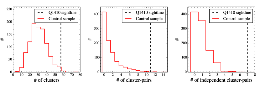
Figure 3: Comparison between our observed (dashed black vertical lines) number of redMaPPer clusters (left panel), cluster-pairs (middle panel) and independent cluster-pairs (right panel) in the Q1410 sightline satisfying our criteria (see Section 3.1, Section 3.2 and Section 3.3, respectively), and the distributions from control samples (solid red histograms; see Section 3.4). The Q1410 sightline is highly exceptional in terms of number of LSS traced by galaxy clusters close to it.

3.4 How unusual is the Q1410 field?

As explained in Section 2.2.1, the field around Q1410 was selected to maximize the presence of cluster-pairs close to the QSO sightline. Therefore, it is by no means a randomly selected sightline. To quantify how unusual the sightline is, we have performed the same search for clusters, cluster-pairs and independent cluster-pairs in $1000$ randomly selected sightlines having coordinates R.A. $\in[140,222]$ degrees and Dec. $\in[4,56]$ degrees (i.e. well within the SDSS footprint), using the same set of criteria used to characterize the Q1410 field (see Section 3.1, Section 3.2 and Section 3.3).

In Figure 3 we compare our observed (dashed black vertical lines) number of redMaPPer clusters (left panel), cluster-pairs (middle panel) and independent cluster-pairs (right panel), to the distributions from our control samples (solid red histograms). There are a total of $57$ clusters at redshifts $0.1\leq z\leq 0.5$ satisfying the condition of being at impact parameter of $<20$ Mpc from the Q1410 sightline, whereas the average random expectation is $32\pm 10$ with median of $32$. Likewise, the actual number of cluster-pairs and independent cluster-pair within our constraints are $11$ and $7$ respectively, whereas the average random expectations are $1.6\pm 2.2$ and $1\pm 1$, with medians of $1$ and $1$, respectively. These last two distributions are very skewed towards zero.

Although the number of clusters around Q1410 exceeds that from the random expectation at only the $2-3\sigma$ confidence level (c.l.), the excesses of total and independent cluster-pairs are highly significant ($>5\sigma$), making Q1410 a very exceptional sightline. We take this fact into account when comparing the incidences of absorption line systems close to cluster-pairs and the field as estimated from the Q1410 sightline itself (see Section 5.2).

4 Characterization of absorption lines in the Q1410 spectrum

We performed a full characterization of absorption lines in the HST/COS FUV spectrum of Q1410. This approach is more time consuming than just restricting ourselves to spectral regions associated with the redshifts where known structures exist (e.g. clusters, cluster-pairs; see Section 3), but is necessary to avoid potential biases and systematic effects. In particular, our approach allows us to: (i) identify absorption lines independently of the presence of known structures; (ii) quantify how the rest of the redshift path unassociated with these known structures compares to the field expectation in terms of absorption features (see Section 5.2); and (iii) assess the extent of contamination by blended unassociated lines in a given redshift. This last point is crucial to minimize misidentification of lines, but some ambiguous cases are unavoidable. In this section we present our methodology for the identification and characterization of absorption lines in the Q1410 spectrum, and how we handled ambiguity.

4.1 Absorption line identification

We searched for individual absorption line components in the continuum normalized QSO spectrum manually (i.e. eyeballing), based on an iterative algorithm described as follows:

Table 4: Absorption lines in the Q1410 sightline.

Component ID	Ion	Obs. wavelength	$z$	$\log(N/$cm${}^{-2})$	$b$	$W_{r}$	$\langle S/N\rangle_{\rm res}$	Label
		(Å)			(km s-1)	(Å)
(1)	(2)	(3)	(4)	(5)	(6)	(7)	(8)	(9)
1	C iv	1547.8	-0.00024 $\pm$ 0.00013	13.98 $\pm$ 0.82	18 $\pm$ 35	0.205 $\pm$ 0.383	14 $\pm$ 1	a
2	Si iv	1393.4	-0.00024 $\pm$ 0.00003	13.38 $\pm$ 0.82	15 $\pm$ 22	0.134 $\pm$ 0.231	12 $\pm$ 1	a
3	Al ii	1670.5	-0.00018 $\pm$ 0.00100	14.13 $\pm$ 40.72	11 $\pm$ 131	0.268 $\pm$ 2.683	11 $\pm$ 1	a
4	N v	1238.6	-0.00018 $\pm$ 0.00011	13.55 $\pm$ 0.53	23 $\pm$ 55	0.064 $\pm$ 0.105	15 $\pm$ 1	a
5	Si iv	1393.6	-0.00014 $\pm$ 0.00008	13.73 $\pm$ 0.38	35 $\pm$ 14	0.304 $\pm$ 0.203	12 $\pm$ 1	a
6	Si iii	1206.4	-0.00012 $\pm$ 0.00003	16.24 $\pm$ 1.53	16 $\pm$ 10	0.534 $\pm$ 1.077	14 $\pm$ 1	a
7	C iv	1548.0	-0.00011 $\pm$ 0.00011	14.09 $\pm$ 0.66	18 $\pm$ 29	0.227 $\pm$ 0.340	15 $\pm$ 1	a
8	Si ii	1260.3	-0.00010 $\pm$ 0.00001	16.58 $\pm$ 0.08	17 $\pm$ 1	0.700 $\pm$ 0.057	16 $\pm$ 1	a
9	C ii	1334.4	-0.00010 $\pm$ 0.00003	18.32 $\pm$ 1.65	23 $\pm$ 9	0.824 $\pm$ 1.500	11 $\pm$ 1	a
10	Al ii	1670.7	-0.00006 $\pm$ 0.00107	14.07 $\pm$ 66.61	9 $\pm$ 204	0.222 $\pm$ 2.217	11 $\pm$ 1	a
11	C ii*	1335.6	-0.00006 $\pm$ 0.00007	14.11 $\pm$ 0.38	24 $\pm$ 32	0.164 $\pm$ 0.188	12 $\pm$ 1	a
12	Si iii	1206.7	0.00019 $\pm$ 0.00004	13.28 $\pm$ 3.99	11 $\pm$ 41	0.121 $\pm$ 0.894	14 $\pm$ 1	a
13	Si iii	1207.2	0.00056 $\pm$ 0.00016	12.37 $\pm$ 0.92	17 $\pm$ 88	0.043 $\pm$ 0.169	13 $\pm$ 1	a
14	H i	1222.7	0.00579 $\pm$ 0.00003	12.86 $\pm$ 0.17	19 $\pm$ 17	0.036 $\pm$ 0.019	13 $\pm$ 1	c
15	H i	1224.7	0.00744 $\pm$ 0.00002	12.90 $\pm$ 0.12	12 $\pm$ 11	0.037 $\pm$ 0.020	14 $\pm$ 1	c
16	H i	1225.0	0.00771 $\pm$ 0.00002	12.92 $\pm$ 0.30	7 $\pm$ 14	0.034 $\pm$ 0.032	14 $\pm$ 1	c
17	H i	1250.5	0.02865 $\pm$ 0.00001	13.49 $\pm$ 0.06	18 $\pm$ 5	0.115 $\pm$ 0.022	16 $\pm$ 1	b
18	H i	1250.9	0.02894 $\pm$ 0.00001	13.57 $\pm$ 0.05	32 $\pm$ 7	0.155 $\pm$ 0.023	16 $\pm$ 1	b
19	H i	1259.4	0.03594 $\pm$ 0.00001	13.74 $\pm$ 0.05	27 $\pm$ 4	0.197 $\pm$ 0.025	16 $\pm$ 1	b
20	H i	1268.9	0.04375 $\pm$ 0.00001	13.49 $\pm$ 9.56	4 $\pm$ 26	0.044 $\pm$ 0.441	15 $\pm$ 1	c
21	H i	1269.4	0.04418 $\pm$ 0.00004	12.93 $\pm$ 0.16	30 $\pm$ 19	0.043 $\pm$ 0.017	15 $\pm$ 1	c
22	H i	1292.0	0.06277 $\pm$ 0.00001	13.32 $\pm$ 0.08	21 $\pm$ 7	0.089 $\pm$ 0.019	14 $\pm$ 1	b
23	H i	1295.9	0.06599 $\pm$ 0.00004	12.86 $\pm$ 0.17	21 $\pm$ 16	0.036 $\pm$ 0.017	14 $\pm$ 1	c
24	H i	1298.3	0.06800 $\pm$ 0.00077	14.32 $\pm$ 6.43	25 $\pm$ 76	0.300 $\pm$ 3.003	14 $\pm$ 1	c
25	H i	1324.8	0.08981 $\pm$ 0.00002	13.29 $\pm$ 0.10	22 $\pm$ 10	0.087 $\pm$ 0.025	10 $\pm$ 1	b
26	H i	1372.7	0.12920 $\pm$ 0.00002	13.55 $\pm$ 0.06	44 $\pm$ 8	0.159 $\pm$ 0.023	12 $\pm$ 1	b
27	H i	1410.9	0.16058 $\pm$ 0.00005	13.40 $\pm$ 0.11	59 $\pm$ 22	0.123 $\pm$ 0.033	14 $\pm$ 1	b
28	H i	1416.4	0.16515 $\pm$ 0.00006	12.80 $\pm$ 0.28	23 $\pm$ 26	0.032 $\pm$ 0.026	14 $\pm$ 1	c
29	H i	1419.3	0.16748 $\pm$ 0.00005	12.76 $\pm$ 0.17	30 $\pm$ 19	0.030 $\pm$ 0.013	16 $\pm$ 2	c
30	H i	1424.7	0.17192 $\pm$ 0.00004	12.88 $\pm$ 0.13	34 $\pm$ 16	0.039 $\pm$ 0.013	19 $\pm$ 2	b
31	H i	1429.4	0.17580 $\pm$ 0.00004	12.86 $\pm$ 0.15	31 $\pm$ 17	0.037 $\pm$ 0.014	22 $\pm$ 2	c
32	H i	1433.2	0.17894 $\pm$ 0.00002	13.07 $\pm$ 0.09	23 $\pm$ 8	0.057 $\pm$ 0.013	21 $\pm$ 4	b
33	H i	1441.1	0.18543 $\pm$ 0.00002	13.00 $\pm$ 0.07	22 $\pm$ 6	0.048 $\pm$ 0.009	24 $\pm$ 1	b
34	H i	1444.1	0.18794 $\pm$ 0.00007	13.41 $\pm$ 0.08	112 $\pm$ 28	0.133 $\pm$ 0.026	23 $\pm$ 2	b
35	H i	1449.9	0.19267 $\pm$ 0.00002	12.91 $\pm$ 0.09	24 $\pm$ 9	0.041 $\pm$ 0.009	23 $\pm$ 2	b
36	C ii	1613.5	0.20904 $\pm$ 0.00001	14.53 $\pm$ 1.73	6 $\pm$ 6	0.096 $\pm$ 0.135	8 $\pm$ 2	a
37	Si ii	1523.9	0.20905 $\pm$ 0.00002	12.54 $\pm$ 0.10	11 $\pm$ 8	0.046 $\pm$ 0.016	16 $\pm$ 1	a
38	H i	1469.8	0.20908 $\pm$ 0.00001	16.15 $\pm$ 1.03	11 $\pm$ 3	0.257 $\pm$ 0.155	18 $\pm$ 1	a
39	Si iii	1458.8	0.20909 $\pm$ 0.00001	12.63 $\pm$ 0.06	13 $\pm$ 4	0.066 $\pm$ 0.011	20 $\pm$ 1	a
40	C iii	1181.4	0.20915 $\pm$ 0.00001	14.60 $\pm$ 13.57	8 $\pm$ 35	0.113 $\pm$ 1.134	12 $\pm$ 1	a
41	N iii	1196.8	0.20916 $\pm$ 0.00002	13.84 $\pm$ 0.10	19 $\pm$ 10	0.060 $\pm$ 0.017	13 $\pm$ 1	a
42	H i	1470.0	0.20920 $\pm$ 0.00030	13.37 $\pm$ 2.72	14 $\pm$ 47	0.088 $\pm$ 0.571	18 $\pm$ 1	a
43	Si ii	1524.5	0.20955 $\pm$ 0.00001	13.05 $\pm$ 0.15	13 $\pm$ 5	0.109 $\pm$ 0.043	15 $\pm$ 2	a
44	C ii	1614.2	0.20955 $\pm$ 0.00001	14.96 $\pm$ 1.42	10 $\pm$ 7	0.174 $\pm$ 0.184	8 $\pm$ 2	a
45	Si iv	1685.8	0.20956 $\pm$ 0.00001	13.67 $\pm$ 0.08	14 $\pm$ 3	0.170 $\pm$ 0.033	10 $\pm$ 1	a
46	H i	1470.5	0.20958 $\pm$ 0.00015	16.29 $\pm$ 3.61	14 $\pm$ 7	0.330 $\pm$ 3.272	18 $\pm$ 1	a
47	N iii	1197.3	0.20962 $\pm$ 0.00001	14.94 $\pm$ 1.48	14 $\pm$ 12	0.151 $\pm$ 0.192	13 $\pm$ 1	a
48	Si iii	1459.4	0.20962 $\pm$ 0.00001	13.56 $\pm$ 0.07	23 $\pm$ 3	0.256 $\pm$ 0.032	20 $\pm$ 1	a
49	C iii	1181.8	0.20964 $\pm$ 0.00236	15.03 $\pm$ 59.37	13 $\pm$ 98	0.188 $\pm$ 1.884	12 $\pm$ 1	a
50	N v	1498.5	0.20964 $\pm$ 0.00003	13.57 $\pm$ 0.09	31 $\pm$ 10	0.071 $\pm$ 0.015	17 $\pm$ 1	a
51	O vi	1248.3	0.20967 $\pm$ 0.00005	14.31 $\pm$ 0.21	26 $\pm$ 10	0.164 $\pm$ 0.073	16 $\pm$ 1	a
52	Si ii	1524.8	0.20973 $\pm$ 0.00005	13.06 $\pm$ 0.16	34 $\pm$ 13	0.150 $\pm$ 0.058	15 $\pm$ 2	a
53	C ii	1614.5	0.20976 $\pm$ 0.00001	14.48 $\pm$ 0.04	20 $\pm$ 3	0.233 $\pm$ 0.029	8 $\pm$ 2	a
54	H i	1470.7	0.20980 $\pm$ 0.00024	15.93 $\pm$ 2.00	27 $\pm$ 15	0.534 $\pm$ 0.567	18 $\pm$ 1	a
55	Si iv	1686.2	0.20981 $\pm$ 0.00002	13.27 $\pm$ 0.07	26 $\pm$ 7	0.128 $\pm$ 0.025	10 $\pm$ 1	a
56	Si iii	1459.7	0.20986 $\pm$ 0.00001	13.17 $\pm$ 0.05	21 $\pm$ 4	0.178 $\pm$ 0.025	20 $\pm$ 1	a
57	C iii	1182.1	0.20986 $\pm$ 0.00021	17.15 $\pm$ 0.78	14 $\pm$ 18	0.488 $\pm$ 0.515	12 $\pm$ 1	a
58	O vi	1248.5	0.20987 $\pm$ 0.00006	14.16 $\pm$ 0.31	26 $\pm$ 16	0.129 $\pm$ 0.095	16 $\pm$ 1	a
59	N iii	1197.5	0.20987 $\pm$ 0.00003	14.09 $\pm$ 0.11	25 $\pm$ 12	0.100 $\pm$ 0.031	13 $\pm$ 1	a
60	H i	1471.3	0.21028 $\pm$ 0.00001	13.70 $\pm$ 0.05	19 $\pm$ 3	0.157 $\pm$ 0.020	18 $\pm$ 1	a
61	O vi	1248.9	0.21028 $\pm$ 0.00001	14.50 $\pm$ 0.03	50 $\pm$ 6	0.270 $\pm$ 0.022	16 $\pm$ 1	a
62	N v	1499.3	0.21029 $\pm$ 0.00006	13.53 $\pm$ 0.15	50 $\pm$ 24	0.068 $\pm$ 0.024	16 $\pm$ 1	a
63	C iii	1182.5	0.21033 $\pm$ 0.00002	13.09 $\pm$ 0.18	11 $\pm$ 11	0.055 $\pm$ 0.040	12 $\pm$ 1	a
64	H i	1478.4	0.21615 $\pm$ 0.00002	13.30 $\pm$ 0.05	42 $\pm$ 7	0.096 $\pm$ 0.012	17 $\pm$ 1	b
65	H i	1481.9	0.21900 $\pm$ 0.00002	13.10 $\pm$ 0.07	36 $\pm$ 9	0.063 $\pm$ 0.011	17 $\pm$ 1	b
66	H i	1486.8	0.22300 $\pm$ 0.00002	13.32 $\pm$ 0.05	52 $\pm$ 8	0.104 $\pm$ 0.012	17 $\pm$ 1	b

(1) Absorption component ID. (2) Ion (see Section 4.1 for details on the line identification process). (3) Observed wavelength of the strongest transition of the ion in the HST/COS spectrum. (4) Redshift from the Voigt profile fitting (see Section 4.2). (5) Column density from the Voigt profile fitting (see Section 4.2). (6) Doppler parameter from the Voigt profile fitting (see Section 4.2). (7) Inferred rest-frame equivalent width from fitted values (note that uncertainties are greatly overestimated for saturated lines or unconstrained fits; see Section 4.3). (8) Averaged local S/N (see Section 4.4). (9) Line reliability flag (‘a’ secure, ‘b’ possible and ‘c’ uncertain; see Section 4.4).

Table 5: continued

Component ID	Ion	Obs. wavelength	$z$	$\log(N/$cm${}^{-2})$	$b$	$W_{r}$	$\langle S/N\rangle_{\rm res}$	Label
		(Å)			(km s-1)	(Å)
(1)	(2)	(3)	(4)	(5)	(6)	(7)	(8)	(9)
67	H i	1497.1	0.23150 $\pm$ 0.00001	13.45 $\pm$ 0.04	32 $\pm$ 4	0.125 $\pm$ 0.012	17 $\pm$ 1	b
68	O vi	1274.5	0.23508 $\pm$ 0.00001	14.08 $\pm$ 0.05	24 $\pm$ 4	0.111 $\pm$ 0.014	15 $\pm$ 1	a
69	H i	1501.5	0.23511 $\pm$ 0.00001	14.48 $\pm$ 0.04	32 $\pm$ 1	0.395 $\pm$ 0.021	17 $\pm$ 1	a
70	H i	1509.0	0.24126 $\pm$ 0.00003	13.29 $\pm$ 0.06	54 $\pm$ 10	0.097 $\pm$ 0.014	16 $\pm$ 1	b
71	H i	1538.8	0.26584 $\pm$ 0.00005	14.91 $\pm$ 0.41	28 $\pm$ 4	0.419 $\pm$ 0.111	15 $\pm$ 1	a
72	C iii	1236.8	0.26587 $\pm$ 0.00001	13.70 $\pm$ 40.19	3 $\pm$ 66	0.041 $\pm$ 0.406	15 $\pm$ 1	a
73	H i	1539.0	0.26593 $\pm$ 0.00001	15.88 $\pm$ 0.06	16 $\pm$ 2	0.328 $\pm$ 0.041	15 $\pm$ 1	a
74	H i	1541.8	0.26827 $\pm$ 0.00010	12.78 $\pm$ 0.22	50 $\pm$ 37	0.032 $\pm$ 0.017	15 $\pm$ 1	c
75	H i	1545.5	0.27132 $\pm$ 0.00004	12.98 $\pm$ 0.12	36 $\pm$ 16	0.049 $\pm$ 0.015	14 $\pm$ 2	b
76	H i	1550.9	0.27574 $\pm$ 0.00004	13.87 $\pm$ 0.32	21 $\pm$ 17	0.200 $\pm$ 0.166	14 $\pm$ 1	c
77	H i	1566.7	0.28874 $\pm$ 0.00007	13.06 $\pm$ 0.15	49 $\pm$ 25	0.059 $\pm$ 0.022	13 $\pm$ 1	c
78	H i †	1573.8	0.29459 $\pm$ 0.00017	13.58 $\pm$ 0.13	157 $\pm$ 57	0.193 $\pm$ 0.058	14 $\pm$ 1	b
79	H i	1576.7	0.29696 $\pm$ 0.00010	12.75 $\pm$ 0.23	45 $\pm$ 37	0.030 $\pm$ 0.017	13 $\pm$ 1	c
80	H i	1578.8	0.29874 $\pm$ 0.00001	13.68 $\pm$ 0.03	36 $\pm$ 4	0.191 $\pm$ 0.015	13 $\pm$ 1	b
81	H i	1582.7	0.30188 $\pm$ 0.00002	13.25 $\pm$ 0.07	32 $\pm$ 8	0.084 $\pm$ 0.014	13 $\pm$ 1	b
82	H i	1584.2	0.30314 $\pm$ 0.00003	13.32 $\pm$ 0.07	47 $\pm$ 11	0.102 $\pm$ 0.017	13 $\pm$ 1	b
83	H i	1613.9	0.32756 $\pm$ 0.00003	13.24 $\pm$ 0.11	24 $\pm$ 11	0.079 $\pm$ 0.024	8 $\pm$ 2	b
84	H i	1617.4	0.33044 $\pm$ 0.00004	13.38 $\pm$ 0.09	45 $\pm$ 13	0.113 $\pm$ 0.024	10 $\pm$ 1	b
85	H i	1631.6	0.34217 $\pm$ 0.00006	13.75 $\pm$ 0.05	153 $\pm$ 19	0.276 $\pm$ 0.030	10 $\pm$ 1	b
86	O vi	1392.6	0.34954 $\pm$ 0.00002	13.77 $\pm$ 0.09	21 $\pm$ 8	0.061 $\pm$ 0.015	11 $\pm$ 1	a
87	Si iii	1628.6	0.34986 $\pm$ 0.00001	13.50 $\pm$ 0.03	45 $\pm$ 4	0.378 $\pm$ 0.032	10 $\pm$ 1	a
88	H i	1641.0	0.34986 $\pm$ 0.00001	15.88 $\pm$ 0.03	17 $\pm$ 1	0.344 $\pm$ 0.015	11 $\pm$ 1	a
89	O vi	1393.0	0.34989 $\pm$ 0.00001	14.07 $\pm$ 0.06	19 $\pm$ 5	0.101 $\pm$ 0.018	11 $\pm$ 1	a
90	C ii	1801.5	0.34989 $\pm$ 0.00001	13.31 $\pm$ 0.36	5 $\pm$ 5	0.030 $\pm$ 0.028	11 $\pm$ 1	a
91	N iii	1336.2	0.34998 $\pm$ 0.00006	14.04 $\pm$ 0.11	50 $\pm$ 20	0.102 $\pm$ 0.028	12 $\pm$ 1	a
92	H i	1641.4	0.35020 $\pm$ 0.00004	14.29 $\pm$ 0.09	97 $\pm$ 10	0.701 $\pm$ 0.116	11 $\pm$ 1	b
93	O vi	1393.4	0.35029 $\pm$ 0.00001	14.48 $\pm$ 0.05	35 $\pm$ 5	0.233 $\pm$ 0.029	12 $\pm$ 1	a
94	H i	1641.6	0.35035 $\pm$ 0.00001	14.57 $\pm$ 0.06	26 $\pm$ 3	0.346 $\pm$ 0.047	11 $\pm$ 1	a
95	H i	1642.4	0.35106 $\pm$ 0.00001	15.43 $\pm$ 0.03	25 $\pm$ 1	0.440 $\pm$ 0.015	11 $\pm$ 1	a
96	H i	1652.3	0.35918 $\pm$ 0.00002	13.61 $\pm$ 0.05	31 $\pm$ 5	0.163 $\pm$ 0.022	11 $\pm$ 1	b
97	H i	1658.1	0.36397 $\pm$ 0.00003	13.52 $\pm$ 0.06	58 $\pm$ 10	0.156 $\pm$ 0.021	11 $\pm$ 1	b
98	H i	1664.1	0.36886 $\pm$ 0.00005	13.25 $\pm$ 0.11	50 $\pm$ 18	0.089 $\pm$ 0.023	11 $\pm$ 1	b
99	H i	1666.8	0.37106 $\pm$ 0.00001	14.06 $\pm$ 0.03	36 $\pm$ 2	0.329 $\pm$ 0.022	11 $\pm$ 1	a
100	H i	1667.6	0.37176 $\pm$ 0.00003	13.24 $\pm$ 0.08	29 $\pm$ 9	0.081 $\pm$ 0.016	11 $\pm$ 1	a
101	H i	1673.8	0.37686 $\pm$ 0.00001	13.59 $\pm$ 0.04	31 $\pm$ 4	0.159 $\pm$ 0.018	11 $\pm$ 1	a
102	O vi	1426.5	0.38238 $\pm$ 0.00002	13.43 $\pm$ 0.14	7 $\pm$ 12	0.026 $\pm$ 0.016	21 $\pm$ 2	c
103	H i	1680.6	0.38242 $\pm$ 0.00005	12.91 $\pm$ 0.16	27 $\pm$ 17	0.041 $\pm$ 0.017	10 $\pm$ 1	c
104	H i	1683.8	0.38508 $\pm$ 0.00001	14.25 $\pm$ 0.03	32 $\pm$ 2	0.345 $\pm$ 0.019	11 $\pm$ 1	a
105	H i	1691.0	0.39097 $\pm$ 0.00007	13.19 $\pm$ 0.14	53 $\pm$ 25	0.078 $\pm$ 0.027	10 $\pm$ 1	c
106	H i	1704.6	0.40219 $\pm$ 0.00012	13.28 $\pm$ 0.20	79 $\pm$ 49	0.097 $\pm$ 0.048	10 $\pm$ 1	c
107	H i	1704.7	0.40224 $\pm$ 0.00003	13.07 $\pm$ 0.30	15 $\pm$ 14	0.053 $\pm$ 0.046	10 $\pm$ 1	c
108	H i	1716.3	0.41182 $\pm$ 0.00005	13.47 $\pm$ 0.09	62 $\pm$ 18	0.142 $\pm$ 0.031	9 $\pm$ 1	b
109	H i	1723.3	0.41758 $\pm$ 0.00001	14.38 $\pm$ 0.03	19 $\pm$ 1	0.254 $\pm$ 0.014	9 $\pm$ 1	a
110	H i	1726.5	0.42022 $\pm$ 0.00006	13.25 $\pm$ 0.12	56 $\pm$ 20	0.090 $\pm$ 0.025	10 $\pm$ 1	b
111	H i	1737.3	0.42911 $\pm$ 0.00008	13.08 $\pm$ 0.15	55 $\pm$ 27	0.062 $\pm$ 0.023	9 $\pm$ 1	c
112	H i	1740.4	0.43167 $\pm$ 0.00005	13.73 $\pm$ 0.83	23 $\pm$ 14	0.179 $\pm$ 0.213	10 $\pm$ 1	a
113	H i	1740.6	0.43183 $\pm$ 0.00083	13.21 $\pm$ 2.74	37 $\pm$ 102	0.079 $\pm$ 0.793	9 $\pm$ 1	c
114	H i	1768.4	0.45466 $\pm$ 0.00006	13.46 $\pm$ 0.08	81 $\pm$ 18	0.143 $\pm$ 0.026	9 $\pm$ 1	b
115	H i	1775.9	0.46085 $\pm$ 0.00035	13.55 $\pm$ 0.25	192 $\pm$ 141	0.185 $\pm$ 0.115	9 $\pm$ 1	c
116	H i	1777.7	0.46235 $\pm$ 0.00002	13.77 $\pm$ 0.07	26 $\pm$ 5	0.199 $\pm$ 0.037	9 $\pm$ 1	a
117	O ii	1281.0	0.53509 $\pm$ 0.00001	13.85 $\pm$ 0.25	10 $\pm$ 10	0.041 $\pm$ 0.033	15 $\pm$ 1	a
118	H i	1574.6	0.53510 $\pm$ 0.00001	16.52 $\pm$ 0.02	16 $\pm$ 1	0.274 $\pm$ 0.010	14 $\pm$ 1	a
119	C ii	2048.6	0.53510 $\pm$ 0.00001	13.30 $\pm$ 0.56	10 $\pm$ 10	0.034 $\pm$ 0.051	14 $\pm$ 1	a
120	O iii	1078.2	0.53512 $\pm$ 0.00001	14.51 $\pm$ 0.25	13 $\pm$ 5	0.078 $\pm$ 0.036	14 $\pm$ 1	a
121	C iii	1499.9	0.53520 $\pm$ 0.00001	13.98 $\pm$ 0.25	19 $\pm$ 4	0.177 $\pm$ 0.054	16 $\pm$ 1	a
122	O iv	1209.3	0.53524 $\pm$ 0.00003	14.22 $\pm$ 0.11	23 $\pm$ 10	0.076 $\pm$ 0.023	13 $\pm$ 1	a
123	H i	1574.8	0.53531 $\pm$ 0.00003	14.99 $\pm$ 0.15	17 $\pm$ 4	0.180 $\pm$ 0.050	14 $\pm$ 1	a
124	H i	1717.1	0.67402 $\pm$ 0.00001	14.80 $\pm$ 0.04	31 $\pm$ 3	0.238 $\pm$ 0.024	9 $\pm$ 1	a
125	C iii	1752.5	0.79372 $\pm$ 0.00003	14.84 $\pm$ 7.41	4 $\pm$ 9	0.065 $\pm$ 0.653	9 $\pm$ 1	a
126	O iv	1412.9	0.79373 $\pm$ 0.00002	14.68 $\pm$ 0.09	20 $\pm$ 5	0.128 $\pm$ 0.032	14 $\pm$ 1	a
127	O iii	1259.8	0.79376 $\pm$ 0.00001	14.41 $\pm$ 14.69	3 $\pm$ 22	0.023 $\pm$ 0.234	16 $\pm$ 1	a
128	H i	1839.9	0.79378 $\pm$ 0.00005	15.55 $\pm$ 0.10	37 $\pm$ 6	0.426 $\pm$ 0.077	16 $\pm$ 1	a
129	C iii	1752.7	0.79396 $\pm$ 0.00002	15.14 $\pm$ 8.93	10 $\pm$ 22	0.151 $\pm$ 1.514	9 $\pm$ 1	a
130	O iv	1413.2	0.79401 $\pm$ 0.00002	15.51 $\pm$ 4.99	9 $\pm$ 15	0.097 $\pm$ 0.831	14 $\pm$ 1	a
131	O iii	1260.0	0.79404 $\pm$ 0.00001	14.59 $\pm$ 0.20	12 $\pm$ 3	0.077 $\pm$ 0.024	16 $\pm$ 1	a
132	H i	1840.2	0.79404 $\pm$ 0.00005	14.91 $\pm$ 0.42	18 $\pm$ 10	0.176 $\pm$ 0.115	16 $\pm$ 1	a

(1) Absorption component ID. (2) Ion (see Section 4.1 for details on the line identification process). (3) Observed wavelength of the strongest transition of the ion in the HST/COS spectrum. (4) Redshift from the Voigt profile fitting (see Section 4.2). (5) Column density from the Voigt profile fitting (see Section 4.2). (6) Doppler parameter from the Voigt profile fitting (see Section 4.2). (7) Inferred rest-frame equivalent width from fitted values (note that uncertainties are greatly overestimated for saturated lines or unconstrained fits; see Section 4.3). (8) Averaged local S/N (see Section 4.4). (9) Line reliability flag (‘a’ secure, ‘b’ possible and ‘c’ uncertain; see Section 4.4).

^†: Could be a very broad H i at redshift $z=0.53531$ instead, but we cannot confirm it with our current data.

1. Identify all possible absorption components (H i and metals) within $\pm 500$from redshift $z=0$, and assign them to the ‘reliable’ category (label ‘a’; see Section 4.5).

2. Identify all possible absorption components (H i and metals) within $\pm 500$from redshift $z=z_{\rm QSO}$, and assign them to the ‘reliable’ category.

3. Identify H i absorption components, showing at least two transitions (e.g.  and  or  and , and so on; i.e. strong H i), starting at $z=z_{\rm QSO}$ until $z=0$, and assign them to the ‘reliable’ category. This identification includes the whole Lyman series covered by the spectrum in a given component.

4. Identify all possible metal absorption components within $\pm 200$from each H i redshift found in the previous step, and assign them to the ‘reliable’ category. When the wavelength coverage allows the detection of multiple transitions of a single ion, we require the relative positions of these to coincide; in the case of multiple adjacent components blending with each other, we require them to have similar kinematic structure across the multiple transitions of the same ion.

5. Identify high-ionization transitions (namely: Ne viii, O vi, N v, C iv, Si iv) showing in at least two transitions, independently of the presence of H i, starting at $z=z_{\rm QSO}$ until $z=0$, and assign them to the ‘reliable’ category.

6. Identify low-ionization transitions (namely: C ii, C iii, N ii, N iii, O i, O ii, Si ii, Si iii, Fe ii, Fe iii and Al ii), showing at least two transitions, independently of the presence of H i, starting at $z=z_{\rm QSO}$ until $z=0$, and assign them to the ‘reliable’ category.

7. Assume all the unidentified absorption features to be H i and repeat step (iv). If metals satisfying the criteria in step (iv) exist, assign the component to the ‘reliable’ category; otherwise assign the component to the ‘possible’ category (label ‘b’; see Section 4.5).

8. For complex blended systems we allowed for the presence of extra heavily blended (hidden) ions, preferentially H i unless a metal ion showing at least one unblended transition exist, and update the identification accordingly. In cases where the metal ion shows at least two unblended transitions, assign them to the ‘reliable’ category. In the rest of the cases (including H i only) assign them to the ‘possible’ category.

We note that we will then degrade some of the components in the ‘possible’ category to the ‘uncertain’ category (‘c’), based on an equivalent width significance criterium in Section 4.5.

For all the identified components, we set initial guesses for their redshifts, column densities ($N$), and Doppler parameters ($b$), which are used as the inputs of our automatic Voigt profile fitting process described in the Section 4.2. We based these guesses on the intensities and widths of the spectral features, keeping the number of individual components to the minimum: we only added a component when there is a clear presence of multiple adjacent local minima or asymmetries. In the case of symmetric and intense H i  absorption lines showing no corresponding H i  absorption (when the spectral coverage and the S/N would have allowed it), this last condition would require the components to have relatively large $b$-values (typically $\gtrsim 40-50$). We warn the reader that this is a potential source of bias, especially for the broad  systems ($\geq 50$) expected to trace portions of the WHIM (but see Section 7.5).

4.2 Voigt profile fitting

We fit Voigt profiles to the identified absorption line components using vpfit . We accounted for the non-Gaussian COS line spread function (LSF), by interpolating between the closest COS LSF tabulated values provided by the Space Telescope Science Institute (STScI) at a given wavelength. We used the guesses provided by the absorption line search (see Section 4.1) as the initial input of vpfit, and modified them when needed to reach converged solutions with low reduced $\chi^{2}$.

When dealing with H i absorption lines, we used at least two spectral regions associated with their Lyman series transitions when the spectral coverage allowed it. This means that for those showing only the  transition, we also included their associated  regions (even though they do not show evident absorption) when available. This last condition provides reliable upper limits to the column density of these components. For strong H i components, we used regions associated with as many Lyman series transitions as possible, but excluding those heavily blended or in spectral regions of poor S/N ($\lesssim 1$ per pixel). For metal transitions we used all spectral regions available.

We fitted absorption line systems starting from $z=z_{\rm QSO}$ until $z=0$. When a given system at redshift $0<z\leq z_{\rm QSO}$ showed strong blends from lower redshifts, we fitted them all simultaneously in a given vpfit iteration (i.e. including all spectral regions associated with them). When a given system at redshift $0<z<z_{\rm QSO}$ showed weak blending from higher redshifts, we allowed vpfit to modify the ‘effective’ continuum by adding the previously found absorption line solutions to it. This last condition accounts for the blending of weak lines (especially from higher order Lyman series)—whose solutions are already well determined—in a more efficient manner than fitting all regions involved simultaneously. In the whole process, we allowed vpfit to add lines automatically when the $\chi^{2}$ and the Kolmogorov-Smirnov test (K-S) test probabilities were below $0.01$ (see vpfit manual for details).

Table 4 shows our final list of identified absorption line components, and their corresponding fits. Unique component IDs are given in the first column to components for each ion (second column). The observed wavelength associated with the strongest transition of an ion is shown in the third column (but note that some ions can show up in multiple wavelengths when having multiple transitions). The fitted redshifts, column densities and Doppler parameters are given in the fourth, fifth and sixth columns respectively. Our final reduced $\chi^{2}$ have an average (and median) of $1.1$. In Figure 14 we show how these fits (red line) compare to the observed spectrum (black line), by means of their residuals (grey dots) defined as the difference between the two (i.e. in the same units as the spectrum). We see how these residuals are mostly distributed within the spectrum uncertainty level (green line).

4.3 Rest-frame equivalent widths

For each component we estimate the rest-frame equivalent width of the strongest transition, $W_{\rm r}$, using the approximation given by Draine (2011, see his equation 9.27), based on their fitted $N$ and $b$ values. The resulting values are given in the seventh column of Table 4. We chose this approach in order to avoid complications when dealing with blended components. We emphasize that passing from $W_{\rm r}\rightarrow(N,b)$ is not always robust when on of the flat part of the curve-of-growth, but passing from $(N,b)\rightarrow W_{\rm r}$ is robust. We compared the results in $W_{\rm r}$ from our adopted approach and that from a direct pixel integration, in a subsample of $10$ unblended and unsaturated lines, and obtained consistent results within the uncertainties.

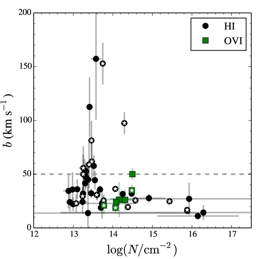
Figure 4: Distribution of Doppler parameters ($b$) as a function of column density ($N$) for H i (black circles) and O vi (green squares) absorption lines found in the HST/COS FUV spectrum between $0.1\leq z\leq 0.5$ and excluding those in category ‘c’ (uncertain; see Section 4.5). White stars mark absorbers associated to cluster-pairs (see Section 5). The horizontal dashed grey line corresponds to a Doppler parameter of $b=50$, our adopted limit to split H i lines into broad and narrow.

The rest-frame equivalent width uncertainty, $\delta W_{\rm r}$, was estimated as follows. We first calculated the maximum/minimum equivalent width, $W_{\rm r}^{\rm max/min}$, still consistent within $1\sigma$ from the $N$ and $b$ fitted values, i.e. using the aforementioned approximation for $(N\pm\delta N,b\pm\delta b)\rightarrow W_{\rm r}^{\rm max/min}$, where $\delta N$ and $\delta b$ are the column density and Doppler parameter uncertainties, respectively, as given by vpfit. We then took $\delta W_{\rm r}\equiv\frac{1}{2}(W_{\rm r}^{\rm max}-W_{\rm r}^{\rm min})$. In catastrophic cases where the fits are unconstrained (i.e. $\delta W_{\rm r}\gg W_{\rm r}$), we arbitrarily imposed $\delta W_{\rm r}=10\times W_{\rm r}$, ensuring a very low significance level.

By using the actual fitted parameters and their corresponding errors, our $\delta W_{\rm r}$ uncertainty estimation takes into account the non-Gaussian shape of the COS LSF (particularly important for broad absorption lines). For saturated lines, our method will give unrealistically large $\delta W_{\rm r}$ uncertainties due to a poor constraint in $N$, which is a conservative choice.

4.4 Local signal-to-noise ratio (S/N) estimation

For each component we estimated the average local spectral signal-to-noise ratio (S/N) per pixel, $\langle S/N\rangle_{\rm pixel}$, over the $50$ closest pixels around its strongest transition, without considering those with flux values below $90\%$ of the continuum. We then estimated the local signal-to-noise ratio (S/N) per resolution element $\langle S/N\rangle_{\rm res}$ as $\sqrt{2}\langle S/N\rangle_{\rm pixel}$. The resulting values are given in the eight column of Table 4.

4.5 Absorption line reliability

To deal with ambiguity and significance of the absorption lines we have introduced a reliability flag scheme as follows:

• Reliable (‘a’): Absorption line components showing at least two transitions or showing up in at least two ions, independently of the significance of its corresponding $W_{\rm r}$.

• Probable (‘b’): Absorption line components showing only one transition, showing up in only one ion, and having $W_{\rm r}/\delta W_{\rm r}\geq 3$.

• Uncertain (‘c’): Absorption line components showing only one transition, showing up in only one ion, and having $W_{\rm r}/\delta W_{\rm r}<3$. Components in this category will be excluded from the main scientific analysis presented in this paper.

This reliability scheme applied to our absorption line list is shown in the ninth column of Table 4. We also show these flags together with the ion component ID given (first column of Table 4) in Figure 14 as vertical labels.

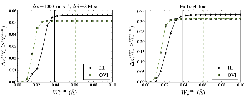
Figure 5: Redshift path, $\Delta z$, as a function of minimum rest-frame equivalent width ,$W_{r}^{\rm min}$, for our survey of H i (black solid line and circles) and O vi (green dashed line and squares) absorption lines. The left panel shows the corresponding redshift path associated to regions of our Q1410 HST/COS spectrum within rest-frame velocity differences $\Delta v=1000$from cluster-pairs at impact parameters smaller than $\Delta d=3$ Mpc. The right panel shows the total corresponding redshift path for the full Q1410 HST/COS spectrum between $0.1\leq z\leq 0.5$. Vertical lines show the minimum rest-frame equivalent width for our detected H i (solid black; $W_{r}=0.039$Å) and O vi (dashed green; $W_{r}=0.061$Å) absorption line samples, excluding those in the category ‘c’ (uncertain; see Section 4.5). See Section 5.1 for further details.

We note that previous studies on broad (BLA) lines have suggested one to quantifying the completeness level of these broad lines by means of $\langle S/N\rangle_{\rm res}\times N/b$ (Richter et al., 2006). The motivation of this criterion is that the BLA is sensitive to both S/N and the optical depth at the line centres, $\tau_{0}\propto N/b$. Therefore, it is not appropriate to use the commonly adopted formalism based on a minimum equivalent width threshold for unresolved lines (these broad lines are usually resolved). In Appendix B we compare the proposed approach by Richter et al. (2006) to ours, and show that imposing a minimum $W_{\rm r}/\delta W_{\rm r}$ value (as defined here) is roughly consistent with imposing a minimum $\langle S/N\rangle_{\rm res}\times N/b$ value for broad lines, but is more conservative when applied to narrow lines. Moreover, our approach has the advantage of being straightforwardly applicable to any absorption line irrespective of its Doppler parameter and ionic transition, hence more appropriate for an homogeneus analysis.

Figure 4 shows the distribution Doppler parameters $b$ as a function of column densities $N$, for our sample of H i (black circles) and O vi (green squares) between $0.1\leq z\leq 0.5$ and excluding those in the ‘c’ category (i.e. uncertain). White stars mark components that lie within $\Delta v\leq 1000$and within impact parameters of $\Delta d\leq 3$ Mpc from cluster-pairs, our fiducial values for associating absorption lines with cluster-pairs (see Section 5).

5 Redshift number density of absorption line systems around cluster-pairs

After having characterized LSS traced by galaxy cluster-pairs around the Q1410 sightline (Section 3) and intervening absorption lines (Section 4), we can now provide a cross-match between the two. Because the completeness level of the redMaPPer clusters with richness $<20$ ($<40$) at $z\sim 0.1-0.4$ ($z\sim 0.4-0.5$) is lower than $\sim 50\%$ (see top panel of fig. 22 of Rykoff et al., 2014), in this paper we will only match absorption lines close to the position of known cluster-pairs rather than the other way around (or both). We also note that the purity of redMaPPer clusters is fairly constant with richness and redshift (some trends are present though), but with values above $95\%$ in all the cases (see bottom panel of fig. 22 of Rykoff et al., 2014); still, the presence of fake clusters will only dilute any real signal when associating absorption lines to inter-cluster filaments traced by cluster-pairs.

In this paper we use the redshift number density of absorption lines, $dN/dz$, as a function of cluster-pair separation, as the relevant statistical quantity to characterize inter-cluster filaments (if any). We have chosen $dN/dz$ as opposed to the number of systems per absorption distance, $dN/dX$, (or both), only for simplicity. Still, in Appendix G we provide tables with relevant quantities and results for both $dN/dz$ and $dN/dX$. We note that our conclusions are independent of this choice.

At this point, it is also important to emphasize that we do not know a priori that cluster-pairs in our sample are tracing true inter-cluster filaments, and that even if they do, we do not know if these could produce a signal in the observed incidences of H i and O vi absorption lines at the S/N level obtained in our Q1410 HST/COS spectrum. Although cosmological hydrodynamical simulations suggest that this may be the case, this paper aims to provide a direct test of such an hypothesis. Therefore, we will explore the behaviour of $dN/dz$ over a wide range of scales around cluster-pairs both along and transverse to the Q1410 LOS. This means that in the following, we will allow the maximum impact parameter for clusters and cluster-pair inter-cluster axes to the Q1410 sightline to be larger than the fiducial values adopted in Section 3.1 and Section 3.2 (i.e. larger than $20$ and $3$ Mpc, respectively).

5.1 Measuring the redshift number density of absorption lines around cluster-pairs

We measure the redshift number density of absorption lines around cluster-pairs in the following way. Let $\Delta d$ be the maximum impact parameter between a cluster-pair inter-cluster axis and the Q1410 sightline in a given calculation. Let $\Delta v$ be the maximum rest-frame velocity window to a given cluster-pair, at the redshift of such cluster-pair (see Figure 1 for an schematic diagram). Then, we define $N(\Delta d,\Delta v,W_{\rm r}^{\rm min})$ as the number of absorption components found within $\Delta v$ from the closest (in rest-frame velocity space) cluster-pair, from those cluster-pairs being within $\Delta d$ from the Q1410 sightline, having rest-frame equivalent widths $W_{\rm r}\geq W_{\rm r}^{\rm min}$. Let $\Delta z(\Delta d,\Delta v,W_{\rm r}^{\rm min})$ be the redshift path in which a given absorption line having $W_{\rm r}\geq W_{\rm r}^{\rm min}$ could have been detected along portions of the spectrum being within $\Delta v$ to any cluster-pair, from those cluster-pairs being within $\Delta d$ from the Q1410 sightline, and being within our redshift range constraint (i.e. $0.1\leq z\leq 0.5$). Then, the redshift number density is calculated as,

$$\frac{dN}{dz}(\Delta d,\Delta v,W_{\rm r}^{\rm min})=\frac{N(\Delta d,\Delta v,W_{\rm r}^{\rm min})}{\Delta z(\Delta d,\Delta v,W_{\rm r}^{\rm min})}\ \rm{.}$$ (3)

Our methodology for estimating $\Delta z(\Delta d,\Delta v,W_{\rm r}^{\rm min})$ is presented in Appendix C.

Figure 5 shows the redshift path, $\Delta z$, along the Q1410 sightline as a function of minimum rest-frame equivalent width ,$W_{r}^{\rm min}$, for our survey of H i (black solid line and circles) and O vi (green dashed line and squares) absorption lines. The left panel shows the corresponding redshift path associated with regions of our Q1410 HST/COS spectrum within rest-frame velocity differences $\Delta v=1000$from cluster-pairs at impact parameters smaller than $\Delta d=3$ Mpc, while the right panel shows the total corresponding redshift path for the full Q1410 HST/COS spectrum between $0.1\leq z\leq 0.5$. We see that the completeness level is very similar between the portions of the spectrum close to cluster-pairs and that of the full spectrum. We checked that this is also the case for multiple choices of $\Delta v$ and $\Delta d$ values, increasing from our fiducial values to cover the full spectrum (not shown). The vertical lines in Figure 5 show the minimum rest-frame equivalent width for our H i (black solid; $W_{\rm r}^{\rm min}=0.039$Å) and O vi (dashed green; $W_{\rm r}^{\rm min}=0.061$Å) absorption line samples, excluding those labelled as ‘uncertain’ (category ‘c’; see Section 4.5). We see that these values correspond to high completeness levels and are therefore adopted as the minimum equivalent widths in the forthcoming analysis (but note that we could have detected O vi down to $W_{\rm r}\sim 0.03$Å with a similar completeness).

5.2 Estimating the field redshift number density from the Q1410 sightline

In this paper we have introduced slightly different ways to count and assess the statistical significance of absorption lines compared with has been done in previous published works. This is so because we opted to do a uniform analysis for H i (either total, broad or narrow) and O vi absorption lines, while previous works have usually focused on one type at a time. Therefore, we estimate the field redshift number density of a given species using our own methodology using the Q1410 sightline data alone. This is justified by the fact that cluster-pair filaments (if any) should only influence specific portions of the spectrum (in our case about $\sim 1/6$ of it), while the rest should match the field expectation (i.e. that from a randomly selected sightline).

As described in section Section 3.4, our sightline is extremely unusual in terms of the number of cluster-pairs close to it (by construction, see also Section 2.2.1). Therefore, an estimation of the field value from this sightline alone could be biased when compared against a representative ensemble of random sightlines. In order to correct for this potential bias we have proceeded as follows. Let $N_{\rm tot}$ be the total number of relevant absorption lines in the full Q1410 sightline between $0.1\leq z\leq 0.5$, and $N_{\rm cpairs}$ be the number of such absorption lines associated with our cluster-pairs assuming fiducial values of $\Delta v=1000$and $\Delta d=3$ Mpc (see Section 5.1 for a definition of these two quantities). Therefore, our expected number of absorption lines associated with the field value can be estimated by,

$$N_{\rm field}\approx N_{\rm tot}-N_{\rm cpairs}\left(1-\frac{n_{\rm cpair}^{\rm field}}{n_{\rm cpair}^{\rm Q1410}}\right)\ \rm{,}$$ (4)

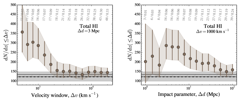
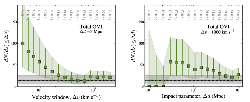
Figure 6: Redshift number density of total H i (brown circles; top panels) and O vi (green squares; bottom panels) absorption components as a function of rest-frame velocity window ($\Delta v$; left panels) and maximum impact parameter to the closest cluster-pair axis ($\Delta d$; right panels) for a fixed $\Delta d=3$ Mpc and $\Delta v=1000$, respectively. Note that bins are not independent from each other, as emphasized by the coloured areas. The total number of lines and redshift paths per bin are given in grey numbers on top of the datapoints. The expected field value estimated from our Q1410 sightline is represented by the horizontal dashed line with its $\pm 1\sigma$ uncertainty represented by the darker grey region. The darkest grey hashed regions represents the $\pm 1\sigma$ field values from the Danforth & Shull (2008) survey. See Section 6.1 for further details.

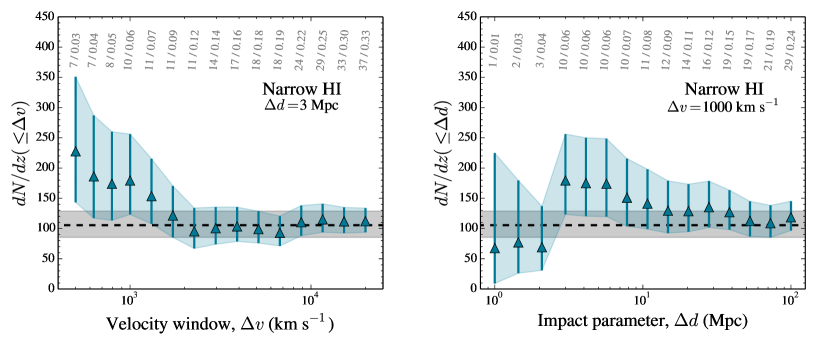
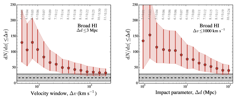
Figure 7: Same as Figure 6 but for narrow ($b<50$; blue triangles; top panels) and broad ($b\geq 50$; red pentagons; bottom panels). The darkest grey hashed regions in the bottom panels represents the $\pm 1\sigma$ field value from the Danforth et al. (2010) BLA survey. See Section 6.1 for further details.

where $n_{\rm cpair}^{\rm Q1410}$ and $n_{\rm cpair}^{\rm field}$ are the number of independent cluster-pairs found in Q1410 sightline and those randomly expected, respectively. In our case $n_{\rm cpair}^{\rm Q1410}=7$ and $n_{\rm cpair}^{\rm field}\approx 1\pm 1$. Therefore, we take the expected field value to be $N_{\rm field}\approx N_{\rm tot}-(0.85\pm 0.14)\ N_{\rm cpairs}$. Finally, we estimate the relevant redshift number density by using this corrected $N_{\rm field}$ as,

$$\frac{dN}{dz}|_{\rm field}=\frac{N_{\rm field}}{\Delta z}\ \rm{,}$$ (5)

where $\Delta z$ is the total redshift path associated with the full Q1410 sightline between $0.1\leq z\leq 0.5$.

This methodology assumes (i) that there is an excess of absorption lines in the data compared to the field expectation, and (ii) that this excess is purely confined within $\Delta v=1000$and $\Delta d=3$ Mpc from the known cluster-pairs. If assumption (i) is incorrect, then our field expectation estimation will be underestimated. If assumption (i) is correct, but assumption (ii) is incorrect, then our field expectation estimation will be overestimated. In Section 6 we show that our field estimations based on Q1410 alone matches those of comparable previously published blind surveys, making our assumptions reasonable.

5.3 Statistical uncertainty estimations

The statistical uncertainty in our calculations is dominated by the uncertainty in $N(\Delta d,\Delta v)$, which we assume is Poissonian and estimate from the analytical approximation given by Gehrels (1986): $\sigma^{+}_{N}\approx\sqrt{N+3/4}+1$ and $\sigma^{-}_{N}\approx\sqrt{N-1/4}$. The statistical uncertainty in our estimation of $N_{\rm field}$ is taken from the contributions of both the Poissonian uncertainty of $N_{\rm tot}$, and the statistical uncertainty of $n_{\rm cpair}^{\rm field}$, which we propagate assuming independence between these two quantities. Given that the statistical uncertainties in $\Delta z(\Delta d,\Delta v)$ and $\Delta X(\Delta d,\Delta v)$ are much smaller, we neglect them.

6 Results

In this section we report our results on $dN/dz$, for our different samples of H i (total, narrow and broad) and O vi absorption lines observed in the Q1410 sightline (see Section 4) applying the methodology described in Section 5 to associate them with cluster-pairs (see Section 3). For simplicity, and in order to reduce the ‘shot noise’ of the measurements, the following results are obtained by varying $\Delta v$ and $\Delta d$ for fixed values of $\Delta d$ and $\Delta v$, respectively (as opposed to varying both values at the same time).

A summary of all the results presented in this section (and those of $dN/dX$, not described here), are given in Tables 7 to 10.

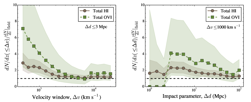
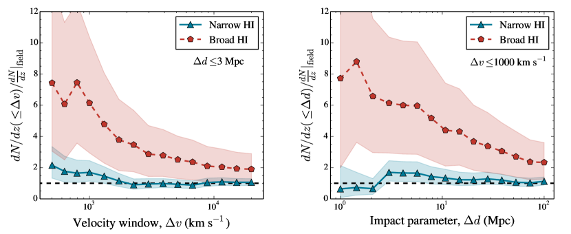
Figure 8: Relative excesses of redshift number densities compared to the field expectation, as a function of rest-frame velocity window ($\Delta v$; left panels) and maximum impact parameter to the closest cluster-pair axis ($\Delta d$; right panels), for fixed $\Delta d=3$ Mpc and $\Delta v=1000$values respectively. The top panels show those for total H i (brown circles, solid lines) and O vi (green squares, dashed lines) absorption line samples. The bottom panels show those for narrow (NLA; $b<50$; blue triangles, solid lines) and broad (BLAs; $b\geq 50$; red pentagons, dashed lines) H i absorption line samples. Coloured light shaded areas represent $\pm 1\sigma$ statistical uncertainties. See Section 6.2 for further details.

6.1 Redshift number densities

Figure 6 shows the $dN/dz$ of total H i (top panels; brown circles) and O vi (bottom panels; green squares) absorption components as a function of maximum velocity window ($\Delta v$; left panels) and maximum impact parameter ($\Delta d$; right panels) for a fixed $\Delta d=3$ Mpc and $\Delta v=1000$, respectively. The expected field values following our approach described in Section 5.2 are shown by the horizontal dashed line with its $\pm 1\sigma$ uncertainty represented by the grey region. We also show the $\pm 1\sigma$ field values from the Danforth & Shull (2008) survey as the darker grey hashed regions, which is consistent with ours.

When we fix $\Delta d=3$ Mpc (left panels), we observe a clear overall increase in the redshift number density of H i and O vi absorption lines with decreasing $\Delta v$. Similarly, when we fix $\Delta v=1000$(right panels), we observe an overall increase in the redshift number density of H i and O vi absorption lines with decreasing $\Delta d$, but only down to $\Delta d\sim 3$ Mpc; at $\Delta d\lesssim 3$ Mpc a flattening (or even decrease) trend is observed, which we believe is mostly due to our small sample in such bins. This change of behaviour motivated our adopted fiducial value of $3$ Mpc for the maximum transverse separation between cluster-pair axis and the Q1410 sightline (see Section 3.2).

To test whether kinematic trends are present in the H i data, we repeated the $dN/dz$ measurements for both narrow (NLA; $b<50$) and broad (BLA; $b\geq 50$) H i absorption lines. Although the canonical value for BLAs tracing the WHIM is $40$, this limit assumes that the broadening is purely thermal. Following more recent work (Richter et al., 2006; Danforth et al., 2010), it is acknowledged that non-thermal broadening mechanisms are likely to be present in absorption line samples. Thus, our adopted value of $b\geq 50$is more conservative (see also Section 7.4).

Figure 7 is equivalent to Figure 6 but for NLA (top panels) and BLA (bottom panels) absorption line samples. The hashed darker grey area in the bottom panels represents the field value obtained by Danforth et al. (2010) for BLAs.

When we fix $\Delta d=3$ Mpc (left panels), we observe a clear overall increase in the redshift number density of both narrow and broad H i absorption lines with decreasing $\Delta v$. When we fix $\Delta v=1000$(right panels), we also observe an overall increase down to $\Delta d\sim 3$ Mpc; below this scale a decreasing trend may be present for narrow H i lines, while for broad H i lines the increasing trend persists.

We also note that our estimation field expectations are fully consistent with those from previous blind surveys (Danforth & Shull, 2008; Danforth et al., 2010). This implies that our characterization of absorption lines (see Section 4) and our methodology for estimating the field expectation from our Q1410 data alone (see Section 5.2) are reasonable. Therefore, we can conclude that the vast majority (if not all) of the observed excesses come from scales within $\Delta v=1000$and $\Delta d=3$ Mpc (see Section 7 for further discussion).

6.2 Relative excesses with respect to the field

Figure 9: Representation of the position of the Q1410 sightline with respect to different independent cluster-pairs in our sample. The $y$-axes correspond to the impact parameter to a given cluster-pair, $\Delta d$, while the $x$-axes correspond to the distance to the closest galaxy cluster in a given cluster-pair, along the cluster-pair axis, $\Delta x$, (see Figure 1 for a schematic diagram). The four panels correspond to different absorption line samples, from top to bottom: total H i   narrow H i (NLAs; $b<50$), broad H i (BLAs; $b\geq 50$), and total O vi. Filled symbols correspond to portions of the sightline showing absorption lines within $\Delta v=1000$from the redshifts of a given cluster-pair, where the sizes of the symbols are proportional to the number of absorption lines. Empty symbols correspond to portions of the sightline showing no absorption. When multiple cluster-pairs lie at similar redshifts (i.e. from grouped ones), the absorption lines are associated to the one having the smallest impact parameter value and the rest of the cluster-pairs are obviated. We also show the typical virial radii of our sample of clusters with a quarter dashed circumference of radii $1$ Mpc centred at the origin. See Section 7.1 for further details.

Figure 8 shows the relative excesses of redshift number densities of our absorption line samples compared to their respective field expectations, defined as $\frac{dN}{dz}/\frac{dN}{dz}|_{\rm field}$, as a function of rest-frame velocity window ($\Delta v$; left panels) and maximum impact parameter to the closest cluster-pair axis ($\Delta d$; right panels), for fixed $\Delta d=3$ Mpc, $\Delta v=1000$, respectively. The top panels show the results for our total H i (brown circles, solid line) and O vi (green squares, dashed line) samples, while the bottom panels show the results for our NLA (blue triangles, solid line) and BLA (red pentagons, dashed line) samples. Coloured light shaded areas represent the $\pm 1\sigma$ statistical uncertainties.

Although subject to large statistical uncertainties, the relative excess for BLAs tends to be the highest of all, reaching a value of $\sim 6$ times its field expectation at $\Delta d=3$ Mpc and $\Delta v=1000$. On the other hand, the excess of NLAs tends to be the smallest of all, reaching a value of only $\sim 1.5$ times its field expectation at the same scales. The relative excess of total H i tends to lie in between that of NLAs and BLAs, but is closer to that of NLAs because these type of absorbers dominate the neutral hydrogen sample. The sample of O vi has the largest statistical uncertainties (it is indeed the smallest sample), which makes its relative excess to be consistent with all others even at the $1\sigma$ c.l. Strictly, within $\sim 2\sigma$ c.l. all the reported excesses are consistent with each other across different samples, and are also consistent with their respective field expectations. Therefore, it is important to test these trends with larger datasets.

6.3 Equivalent widths distributions

In Appendix D we provide a comparison between equivalent widths distributions for our different samples. We did not find statistically significant differences between systems close to cluster-pairs and the field expectation in terms of equivalent widths, at least from our limited sample sizes.

7 Discussion

7.1 Filamentary structure

Here we argue that our results are roughly consistent with a filamentary structure for the absorbing gas close to cluster-pairs. This is so because when we restrict the analysis to a fixed $\Delta v=1000$, the excess is maximized at impact parameters of $\Delta d\sim 3$ Mpc (or even $\Delta d\lesssim 3$ Mpc for broad H i), while the typical separation between clusters in our cluster-pairs are of the order of $\gtrsim 10-15$ Mpc (see sixth and seventh column of Table 3). Moreover, we have also found that when we consider scales far outside our fiducial values, we fully recover the field expectation (see reasoning presented in Section 5.2). From the cumulative results presented in Section 6, we can directly calculate $dN/dz$ in independent intervals instead by subtracting both the reported number of absorption lines and redshift path in a given bin (i.e. $N_{\rm bin}$ and $\Delta z_{\rm bin}$) of a smaller scale, to those at the scale of interest. For instance, if we focus on the total H i sample and consider scales between $3$ to $100$ Mpc as those of interest, we can estimate $dN/dz$ as $\frac{dN}{dz}\sim\frac{(38-16)}{(0.25-0.06)}\sim\frac{22}{0.19}\sim 116\pm 25$ (see top panel of Figure 6 and Table 7). This number is fully consistent with the field expectation (e.g. Danforth & Shull, 2008), and therefore we conclude the vast majority (if not all) of the observed excesses come from scales within $\Delta v=1000$and $\Delta d=3$ Mpc. However, because we did not impose a minimum distance between the QSO sightline and the closest cluster of a cluster-pair, there is also the possibility that our survey geometry does not represent that of a filamentary structure. If those separations are all $\lesssim 3$ Mpc for instance, our survey could be probing a more spherical (or disk) geometry instead.

Figure 9 shows a geometrical representation of our survey. We observe that the distances probed by our survey cover scales between $\Delta x\sim 0-10$ Mpc along the inter-cluster axes, roughly uniformly. Therefore, we conclude that the geometry of our survey is indeed consistent with that of a filamentary structure, but we also stress that a larger sample must be analysed in order to better constrain the geometry.

7.2 Covering fractions of absorbing gas close to cluster-pairs

Here we provide a first estimation of the covering fractions, $f_{c}^{\rm flmnt}$, of the absorbing gas close to cluster-pairs and compare them with the random expectation, $f_{c}^{\rm rand}$. Our adopted fiducial $\Delta v=\pm 1000$corresponds to $\sim\pm 16$ Mpc along the line-of-sight (if cosmological). This is a larger scale compared to our fiducial filament radius of $\sim 3$ Mpc. Therefore, the excesses do not necessarily come from single inter-cluster filaments. Although our reported $dN/dz$ signals tend to keep increasing at smaller rest-frame velocity differences, the samples also get smaller, which makes the statistical uncertainties larger too (see Figures 6 and 7). By comparing the observed covering fractions to random expectations, we can shed light into the origin of the reported excesses in relation to the cluster-pairs themselves.

From Figure 9 we observe that $7/7$ sightlines close to cluster-pairs did show at least $1$ H i absorber, which implies a covering fraction of $f_{c}^{\rm flmt}({\rm HI})\sim 1.00^{+0.00}_{-0.23}$. Similarly, NLAs and BLAs were both found in $5/7$ of the sightlines probing them (although different subsamples; see second and third panel of Figure 9), implying $f_{c}^{\rm flmt}({\rm NLA})\approx f_{c}^{\rm flmt}({\rm BLA})\approx 0.71^{+0.18}_{-0.26}$. In contrast, O vi absorbers were found in $1/7$ of the sightlines probing them, implying a smaller covering fraction of $f_{c}^{\rm flmt}({\rm OVI})\approx 0.14^{+0.26}_{-0.12}$. These results are summarized in Table 6 (upper half) and shown in LABEL:{fig:fcs} (filled symbols), using the same symbol/colour convention as in previous figures.

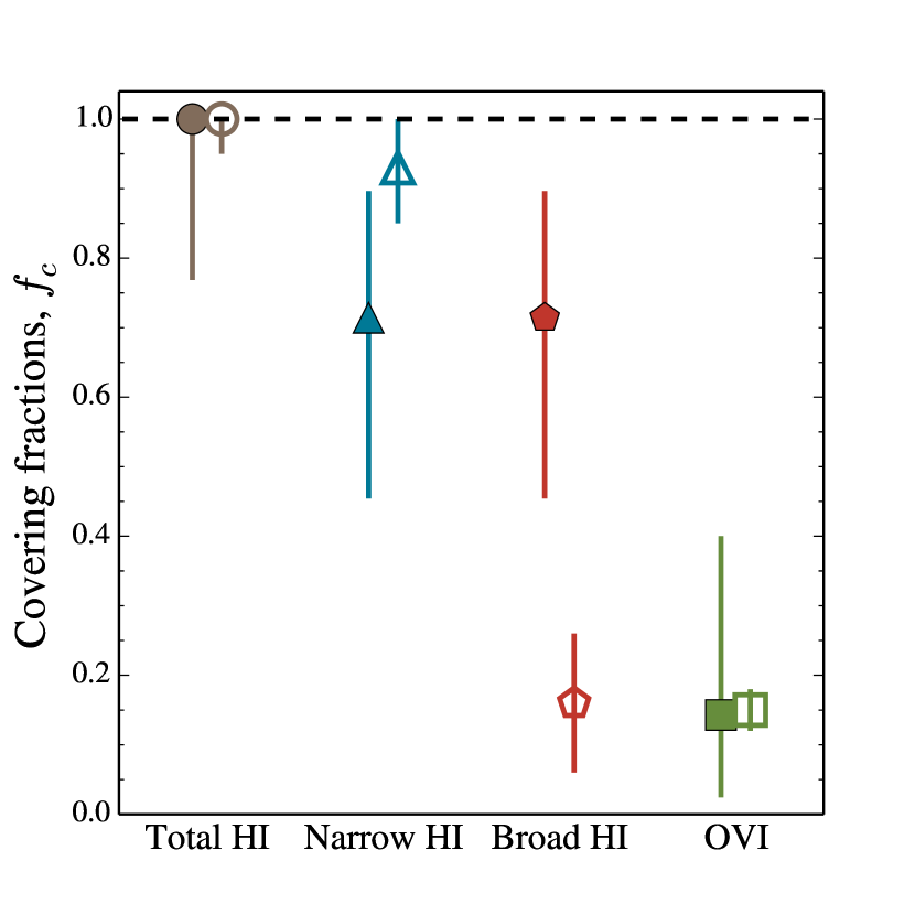
Figure 10: Estimated covering fractions of gas close to cluster-pairs ($f_{c}^{\rm flmnt}$; solid symbols) and in the random expectation ($f_{c}^{\rm rand}$; open symbols), for our different samples of absorption lines using the same symbol/colour convention as in previous figures. We observe that broad H i absorbers ($b\geq 50$) have about $\sim 4$ times a larger covering fraction in close to cluster-pairs than from the random expectation. See Section 7.2 for further details.

As a control sample for a given absorber, we estimated $f_{c}^{\rm rand}$ as,

$$f_{c}^{\rm rand}=\left\{\begin{array}[]{ll}\Delta z({\Delta v})\ \frac{dN}{dz}|_{\rm field}&\mbox{if }\Delta z({\Delta v})\frac{dN}{dz}|_{\rm field}<1\\ 1&\mbox{if }\Delta z({\Delta v})\frac{dN}{dz}|_{\rm field}\geq 1\\ \end{array}\right.$$ (6)

where $\frac{dN}{dz}|_{\rm field}$ is the redshift number density of lines in the field, and $\Delta z(\Delta v)$ is the corresponding redshift path to a rest-frame velocity window $\Delta v$ evaluated at $z=0.35$ (the median redshift of our cluster-pair sample). We note that we are neglecting the intrinsic clustering of absorption lines with themselves, which is justified because our $f_{c}^{\rm flmt}$ estimations are obtained from independent structures.. The fifth column of Table 6 (upper half) summarizes the random expectations for our different samples using $\Delta v=\pm 1000=2000$. These results are also shown in Figure 10 as open symbols. We observe that the covering fractions for total H i, NLAs and O vi close to cluster-pairs are consistent with their random expectations, while $f_{c}^{\rm flmt}({\rm BLA})$ is about $\sim 4$ times larger than its random expectation (at the $\sim 2\sigma$ c.l.). Having consistency with the random expectations are not surprising; as mentioned, $\Delta v=\pm 1000$corresponds to about $\sim\pm 16$ Mpc along the line-of-sight (if cosmological) around massive structures traced by galaxy cluster pairs. In this scenario, we do expect that the $dN/dz|_{\rm field}$ values to be dominated by absorption lines found in the overdense LSS. On the other hand, having an excess in the covering fractions of BLAs with respect to the random expectation implies that this type of gas is not common over $\sim\pm 16$ Mpc scales around cluster-pairs, and therefore it has to come from smaller scales (i.e the cluster-pair itself). To test this hypothesis, we have repeated the covering fractions estimations using a smaller $\Delta v=\pm 500$, and the excess of BLAs remains large ($\sim 7$; see values in the bottom half of Table 6). This behaviour favours the conclusion that most of the BLAs in our sample are directly related to the cluster-pairs themselves.

Table 6: Estimated covering fractions of absorbing gas close to cluster-pairs.

Sample	$n_{\rm hits}$	$n_{\rm trials}$	$f_{c}^{\rm flmnt}$	$f_{c}^{\rm rand}$	Excess
(1)	(2)	(3)	(4)	(5)	(6)
$\Delta v=\pm 1000$and $\Delta d=3$ Mpc
H i	7	7	$1.00^{+0.00}_{-0.23}$	$1.00^{+0.00}_{-0.05}$	$\sim 1$
NLA	5	7	$0.71^{+0.18}_{-0.26}$	$0.93^{+0.07}_{-0.08}$	$\sim 1$
BLA	5	7	$0.71^{+0.18}_{-0.26}$	$0.16^{+0.10}_{-0.10}$	$\sim 4$
O vi	1	7	$0.14^{+0.26}_{-0.12}$	$0.15^{+0.03}_{-0.03}$	$\sim 1$
$\Delta v=\pm 500$and $\Delta d=3$ Mpc
H i	5	7	$0.71^{+0.18}_{-0.26}$	$0.58^{+0.03}_{-0.03}$	$\sim 1$
NLA	3	7	$0.43^{+0.25}_{-0.22}$	$0.47^{+0.04}_{-0.04}$	$\sim 1$
BLA	4	7	$0.57^{+0.22}_{-0.25}$	$0.08^{+0.05}_{-0.05}$	$\sim 7$
O vi	1	7	$0.14^{+0.26}_{-0.12}$	$0.08^{+0.02}_{-0.02}$	$\sim 1$

(1) Sample of absorbing gas. (2) Number of ‘hits’ defined as sightlines showing absorption in a given sample, within $\Delta v=\{\pm 1000,\pm 500\}$and within $\Delta d=3$ Mpc. (3) Number of ‘trials’ defined as the total number of sightlines to look for absorption. (4) Covering fraction close to cluster-pairs estimated as $n_{\rm hits}/n_{\rm trials}$ (uncertainties correspond to those of a binomial $1\sigma$ c.l.). (5) Covering fraction in a random sightline for a given $\Delta v=\{\pm 1000,\pm 500\}$. (6) Excess covering fraction defined as $f_{c}^{\rm flmnt}/f_{c}^{\rm rand}$.

7.3 Could the observed excesses of gas be due to galaxy clusters/groups or individual galaxy halos?

Regarding massive structures, we can see from Figure 9 that the vast majority of sightlines are probing regions far away from the virial radii of known galaxy clusters (see also the left panels of Figure 19). However, because of the limited completeness level of the redMaPPer catalog, there could still be unknown clusters or groups in such regions. In order to directly address this question, one must survey the Q1410 field for individual galaxies and LSS close to the Q1410 line-of-sight, which we leave for future work (see Section 7.6). Still, in the following we provide an assessment of the plausible incidence of gas associated to individual halos from two indirect but independent arguments.

7.3.1 Redshift number density of galaxies

Based on the reasoning presented by Prochaska et al. (2011), one can estimate the redshift number density of galaxies of luminosity $L\geq L_{\rm min}$, $dN/dz|_{\rm gals}$, intersecting a given LOS by assuming a given cross-section for them. For galaxies with $L\geq 0.01-0.001L^{*}$ and assuming cross-sections given by the virial radius of galaxies with unity covering fractions, Prochaska et al. (2011) find that $dN/dz|_{\rm gals}\approx 10-20$ (see their figure 8). This estimate is valid for the field and so we need to correct for the fact that cluster-pairs generally probe LSS overdensities. We use the excess of narrow H i lines to estimate the overall overdensity in our cluster-pair sample, as $\sim 1-2$ times the mean density of the Universe (note that these values are consistent with the expected overdensities traced by cluster-pairs from cosmological simulations). Therefore, we estimate $dN/dz|^{\rm flmnt}_{\rm gals}\approx 10-40$. This number is lower than the typical $dN/dz\sim 60-300$ observed for our samples of H i (either narrow or broad), but is comparable to the $dN/dz\sim 30-100$ observed for O vi. Therefore, it seems unlikely that most of the excess observed for narrow and broad H i gas close to cluster-pairs is driven by galaxy halos of individual galaxies. On the other hand, our reported excess of O vi gas might well be produced (at least partly) by individual galaxy halos (see also below).

7.3.2 Metal absorption lines

One can also infer the presence of galaxy halo material by means of metal absorption lines, in particular from low-ionization species (e.g. Werk et al., 2014). There is only $1$ absorption system in our cluster-pair sample showing metal absorption lines: the one at $z\approx 0.35$ from which all the $3$ observed O vi components come from (see the fourth panel in Figure 19). This system has strong H i absorption with column densities $N>10^{14}$ cm^-2 and shows a complex kinematic structure ($4$ components in total, $3$ narrow and $1$ broad). The second narrow component also shows the presence of C ii, Si iii and N iii (see Table 4). Therefore, although it seems very likely that an important fraction of the absorbing gas in this system comes from an individual galaxy halo or its immediate surroundings, this system only accounts for $3/10\sim 30$ per cent of NLAs and $1/6\sim 16$ per cent of BLAs in our sample. Again, from this independent reasoning we reached the same conclusion as before, i.e. individual galaxy halos could account for the observed excess in O vi lines (although not a requirement), but not for the majority of H i gas.

7.4 Statistical evidence of the WHIM

Here we consider whether the observed trends could also be consistent with the presence of a warm-hot intergalactic medium (WHIM). Ideally, one would require a full characterization of the physical conditions of individual absorbers using multiple species and comparing them with the expectations of different models of ionization. However, because our sample is dominated by absorption systems having no other species than H i, this approach is not feasible. Even when other species are present in individual systems (e.g. H i and O vi) this approach requires the uncertain assumption that the majority of the gas comes from a single phase, which is controversial at the very least (e.g. Werk et al., in prep.). In view of this intrinsic limitation for an individual characterization, here we opted for a purely statistical approach.

The WHIM is usually defined as gas at temperatures in the range of $T\sim 10^{5}-10^{7}$ K, implying a minimum Doppler parameter of $b=40$for H i (i.e. assuming the broadening is purely thermal). Therefore, H i lines with $b<40$can not be caused by a WHIM. Non-thermal processes can also broaden absorption line profiles, including turbulence, Hubble broadening and unresolved blends (e.g. Garzilli et al., 2015, and references therein). In overdense environments, we expect turbulence to be the dominant source of non-thermal physical broadening (but see Section 7.5 for a discussion regarding unresolved blends). Assuming that the turbulence contribution is higher for hotter gas, we should have $b_{\rm turb}\approx\alpha b_{T}$, and hydrodynamical simulations suggest $0\leq\alpha\leq 1$ (e.g. Tepper-García et al., 2012). Assuming the most extreme case of $\alpha=1$, we have that the observed Doppler parameter would be $b=\sqrt{2}b_{T}$, making a limit $b>40\sqrt{2}\approx 57$extremely conservative in ensuring to trace H i gas at $T>10^{5}$ K. However, there could still be genuine WHIM H i absorption lines in the $40<b_{\rm lim}<40\sqrt{2}$range (i.e. when thermal broadening does dominate).

In this paper, we used a limiting Doppler parameter value of $b_{\rm lim}=50$instead, which is in between $40<b_{\rm lim}<40\sqrt{2}$. This limit was partly chosen for allowing a direct comparison to previous published work (e.g. Danforth et al., 2010), but also because it minimizes potential misidentification of lines that are supposed to trace warm-hot gas but trace cool gas instead, and viceversa (i.e. genuine warm-hot absorbers having $b<b_{\rm lim}$, and genuine cool absorbers having $b\geq b_{\rm lim}$). Indeed, using $b_{\rm lim}=50$, there is only $1$ ($1$) line in the range $40<b<50$($50<b<40\sqrt{2}$) in our NLA (BLA) sample associated with cluster-pairs (e.g. see points with white stars in Figure 4). A limit of $b_{\rm lim}=50$also corresponds to a $\alpha=0.75$, and therefore is still quite conservative in ensuring that BLAs trace gas at $T\geq 10^{5}$ K, even with a substantial turbulence contribution. Regardless of these considerations, we also note that about half of the BLAs associated with cluster-pairs in our sample are actually very broad, with Doppler parameters $b\sim 80-150$(e.g. see Figure 4), which should make them more likely to trace gas at WHIM temperatures (but see Section 7.5).

One of our proposed diagnostics is to compare the excesses in the incidence of narrow and broad H i absorbers (and eventually O vi when larger samples are gathered) found close to cluster-pairs with respect to their field expectations (see Figure 8). Because inter- cluster filaments correspond to overdense regions in the Universe, an excess of gas is generally expected to occur, and indeed we have shown that this is the case (see Section 6). Under the null-hypothesis that BLAs and NLAs probe gas in similar physical conditions (i.e. similar physical entities), then we expect both these excesses to behave in a consistent manner. On the other hand, if BLAs and NLAs are not probing similar physical conditions, a different behaviour for the excesses is expected instead. A WHIM signature associated with inter-cluster filaments may include the relative excess of BLAs to be higher than that of NLAs, which is exactly what we observed (although only at the $\sim 1\sigma$ c.l.; see Figure 8, bottom panels). By increasing the sample sizes we may test for any statistically significant difference between them.

Another proposed diagnostic is to constrain the overall geometry for the excess of gas, in terms of both BLAs and NLAs (and O vi when larger samples are gathered). A WHIM signature in this context would require an increase in the covering fractions of BLAs towards the inter-cluster axes compared to the random expectations, which is also what we have observed (again, only at the $\sim 2\sigma$ c.l.; see Section 7.2). Moreover, one can also look for trends in the Doppler parameters of H i absorption lines with respect to impact parameter to the inter-cluster axes, as a proxy of temperature. Assuming simple models for the ionization of the gas (e.g. purely collisional), one can even use the inferred temperatures to estimate a total hydrogen column density from the observed H i one. A WHIM signature should produce, on average, higher hydrogen column densities for higher temperatures.

Although all our tentative results ($\sim 1-2\sigma$ c.l.) may be consistent with the presence of a WHIM in inter-cluster filaments, we emphasize that a larger sample must be analysed before reaching a definite conclusion.

7.5 Caveat

Probably the most important source of concern in our experimental design, is our limited ability to disentangle blends, which is key to detect broad and shallow absorption features expected to arise in the WHIM. The importance of this systematic uncertainty depends on the S/N, as the higher the S/N the easier it is to assess the kinematic structure of the absorption feature (e.g. Richter et al., 2006; Danforth et al., 2010). We emphasize that this is an intrinsic limitation of the absorption-line technique, meaning that all these kind of observational samples are, to some extent, affected by this issue. As described in Section 4, we attempted to avoid this bias by fitting asymmetric lines with at least two components. Although not impossible, we believe that the likelihood of having misidentified multiple narrower blended components as a single broader and symmetric one in a large fraction of our H i sample is low (see Figure 19 for individual examples close to cluster-pairs). Given that we are comparing the relative incidences of lines between different samples drawn from spectra of similar S/N (see Section 6), our statistical approach seems adequate for minimizing this potential source of uncertainty (as opposed to attempting a full physical characterization of individual systems).

7.6 Future prospects

Despite our promising results, the existence of the WHIM in inter-cluster filaments still needs to be observationally confirmed; our pilot survey was not design to draw statistically significant results, but primarily to show that such a goal is currently possible with existing instrumentation. In this section, we enumerate remaining work for providing a firm detection of the elusive WHIM in the context of our methodology.

7.6.1 Increase the sample sizes

Increasing the sample sizes is a key requirement. In this respect, we are actively working on two fronts: (i) pursuing new HST/COS observations of targeted QSO sightlines intersecting multiple cluster-pairs; and (ii) searching in the HST archive for already observed QSOs whose sightline intersects single or multiple cluster-pairs. We estimate that the HST/COS archive will allow us to extend the present work to tens of sightlines, but approach (i) will still be necessary for efficient follow up observations (e.g. galaxy surveys; see Section 7.6.2).

7.6.2 Survey for galaxies around the QSO sightline

As discussed in Section 7.3, we need to survey galaxies around our QSO sightline in order to directly rule out the potential association of BLAs with the halos of individual galaxies. To this end, spectroscopic redshifts are needed (current galaxy photometric redshift uncertainties are too large for meaningful associations with absorption lines). We are currently pursuing multi-object spectroscopy (MOS) and integral field units (IFU) observations around the Q1410 field. We will use MOS surveys to assess the distribution of galaxies over $~{}0.3-10$ Mpc scales. This will be important not only for determining whether galaxy groups or clusters are responsible of our observed excesses of absorbing gas, but also to determine the actual geometry of the LSSs intersected by the Q1410 sightline, including: (i) assess whether these putative inter-cluster filaments are straight or bent; and (ii) refine the cosmological redshift of the structures at the position of the Q1410 sightline. The IFU observations will primarily focus on mapping galaxies on scales within $\lesssim 100-300$ kpc to the QSO sightline (the typical CGM scales) at a very high completeness level, including faint star-forming galaxies with no detectable continuum but having bright enough emission lines.

7.6.3 Comparison to hydrodynamical simulations

Another key aspect of this project, is the comparison of our observational results to those obtained from cosmological simulations. Our experimental design offers a unique opportunity to test the prediction of the $\Lambda$CDM paradigm in the largest and densest filaments of the cosmic web, while also constraining current galaxy evolution models. As we have shown, H i dominates the gaseous content found in inter-cluster filaments (see Section 6), and is very likely that they originate far away from individual galaxy halos (see Section 7.3). This makes a direct comparison to simulations straightforward because we expect this gas to be unaffected by the uncertain baryonic processes occurring in galaxies (e.g. SNe/AGN feedback). On the other hand, the subsample of absorption systems showing metal absorption (e.g. those with O vi) can put constraints on these uncertain ‘sub-grid physic’ models for galaxy formation. However, the need for a full treatment of shocks in the gas limits the approach to being hydrodynamical. If the predictions of WHIM signatures in inter-cluster filaments match our observational results, they will provide yet another piece of evidence supporting the existence of this elusive medium.

8 Summary

The warm-hot intergalactic medium (WHIM) has been predicted to account for a significant fraction of the baryons at low-$z$, but its actual existence has eluded a firm observational confirmation. In this paper, we have presented a novel approach for detecting the WHIM, by targeting regions of the cosmic web where its presence is predicted to be ubiquitous: the putative filaments connecting galaxy clusters. As a proof of concept, we selected a single bright QSO (namely Q1410), whose exceptional sightline passes within $\Delta d=3$ Mpc from the $7$ inter-cluster axes connecting $7$ independent cluster-pairs at redshifts $0.1\leq z\leq 0.5$, and observed it with HST/COS. We performed a full characterization of absorption features in the FUV spectrum of Q1410, independently of the presence of known LSS traced by the galaxy cluster-pairs. From this dataset, we conducted a survey of diffuse gas along the QSO sightline with special focus on H i and O vi absorption lines. This survey allowed us to provide, for the first time, a systematic and statistical measurement of the incidence, $dN/dz$, of intervening H i and O vi absorption lines close to cluster-pairs. We split the sample of H i into broad (BLA) and narrow (NLA) using a Doppler parameter limit of $b_{\rm lim}=50$, which ensures BLAs to be mostly from gas at temperatures $T\geq 10^{5}$ K, even when accounting for turbulence. We quantified the incidence of H i, NLAs, BLAs and O vi absorption lines close to cluster-pairs by varying the minimum rest-frame velocity window, $\Delta v$, and the minimum impact parameter to the inter-cluster axes, $\Delta d$, and found that the incidence of diffuse gas is maximized at $\Delta v\lesssim 1000$and $\Delta d\lesssim 3$ Mpc. At these scales we report:

• $dN/dz({\rm HI})|_{\rm flmnt}=287^{+91}_{-71}$, which corresponds to $2.3^{+0.8}_{-0.6}$ times the field expectation;

• $dN/dz({\rm NLA})|_{\rm flmnt}=179^{+77}_{-56}$ which corresponds to $1.7^{+0.7}_{-0.6}$ times the field expectation;

• $dN/dz({\rm BLA})|_{\rm flmnt}=108^{+65}_{-43}$ which corresponds to $6.1^{+4.2}_{-3.2}$ times the field expectation; and,

• $dN/dz({\rm OVI})|_{\rm flmnt}=58^{+57}_{-32}$ which corresponds to $4.1^{+4.3}_{-2.7}$ times the field expectation.

Although individually these excesses are only at the $\sim 1-2\sigma$ c.l., in concert they suggest a physical overdensity close to cluster-pairs. Our results are also roughly consistent with a filamentary geometry for the absorbing gas connecting cluster-pairs, with covering fractions of: $f_{c}({\rm HI})|_{\rm flmnt}=1.0^{+0.0}_{-0.2}$; $f_{c}({\rm NLA})|_{\rm flmnt}=0.7^{+0.2}_{-0.3}$; $f_{c}({\rm BLA})|_{\rm flmnt}=0.7^{+0.2}_{-0.3}$; and $f_{c}({\rm OVI})|_{\rm flmnt}=0.14^{+0.3}_{-0.1}$. Our resported covering fractions of total H i, NLAs and O vi are all consistent with their random expectations. In contrast, the reported covering fraction of BLAs is a factor of $\sim 4$ larger than the random expectation. Because a rest-frame velocity window of $\Delta v\approx\pm 1000$corresponds to a rather large co-moving distance along the LOS (i.e $\sim\pm 16$ Mpc), having consistency with the random expectation is not surprising, and suggests that most of the excesses of NLAs and O vi absorption come from the overall LSS overdensities around massive structures traced by galaxy cluster pairs. On the other hand, a higher covering fraction of BLAs close to cluster-pairs compared to the random expectation, suggests that the excess of BLAs is physically associated to the cluster-pairs themselves. Indeed, we also reported covering fractions using a $\Delta v\approx\pm 500$and reached the same conclusion.

Based on statistical arguments, we also concluded that most of the reported excesses of NLAs and BLAs cannot be attributed to individual galaxy halos but rather to truly intergalactic material. In contrast, the reported excess of O vi most likely comes from gas associated to individual galaxy halos or their immediate surroundings.

We argued that a behaviour in which BLAs show larger relative excesses compared to that of NLAs (as tentatively reported here), may be a direct signature of the WHIM, especially if identified in the regions close to cluster-pairs. With a larger sample of QSOs and a careful accounting of systematic effects, the technique we have presented here should therefore enable a firm detection of the WHIM in inter-cluster filaments.

Appendix A Properties of clusters close to Q1410 compared to a control sample

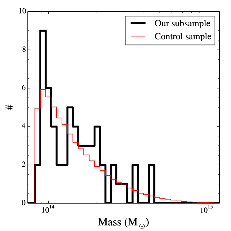
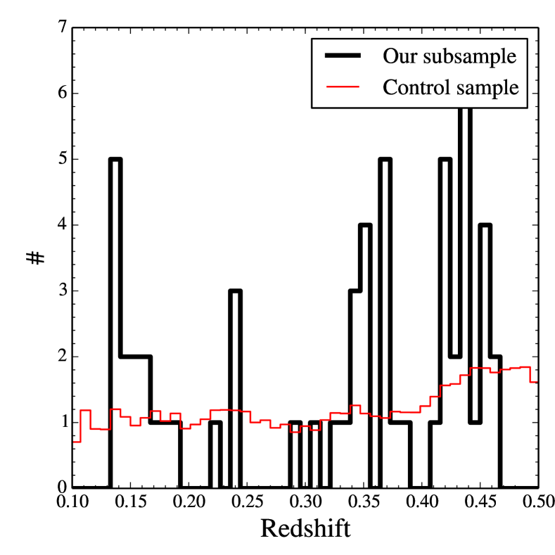
Figure 11: Comparison between mass (left panel) and redshift (right panel) distributions between our subsample of $57$ redMaPPer clusters within $20$ Mpc from the Q1410 sightline, having richness values $\geq 10$ and lying between $0.1\leq z\leq 0.5$ (thick black line), and normalized control samples satisfying only the richness and redshift range criteria (thin red line; see Appendix A for details). A Kolmogorov-Smirnov test to the unbinned distributions give no statistically significant differences between the samples.

In this section we investigate whether our subsample of clusters close to the Q1410 sightline is a fair representation of the cluster population in the whole redMaPPer catalog. To do so, we will compare the mass (estimated from Equation 1) and redshift distributions of our sample to appropriate control samples drawn from the redMaPPer catalog.

The left panel of Figure 11 shows the mass distribution for our subsample of $57$ clusters within $20$ Mpc of Q1410, having richness values $>10$ and lying between $0.1\leq z\leq 0.5$ (thick black line), and the normalized mass distribution from a control sample satisfying only the richness and redshift range criteria ($162\,144$ clusters in total; thin red line). We see no apparent difference between these two distributions, and no statistically significant differences are detected either: the Kolmogorov-Smirnov test over the full unbinned samples gives a $\approx 60\%$ probability of both being drawn from the same parent distribution.

In the case of the redshift distribution, we can not directly compare that of the $162\,144$ clusters satisfying only the richness and redshift range criteria, to our subsample. This is so because our subsample of clusters are defined by a cylinder (i.e. constant volume as a function of redshift), rather than fixed solid angle (increasing volume as a function of redshift). In order to provide an appropriate control sample, we looked at the redshift distribution of redMaPPer clusters having richness values $>10$ and lying between $0.1\leq z\leq 0.5$, in $5000$ cylinders of radius $20$ Mpc, selected at random positions between R.A. $\in[140,222]$ degrees and Dec. $\in[4,56]$ degrees (i.e. well within the SDSS footprint). The right panel of Figure 11 shows the redshift distribution for our subsample of $57$ clusters (thick black line), and the normalized redshift distribution from our aforementioned control sample (thin red line). Again, no statistically significant difference is detected: the Kolmogorov-Smirnov test over the full unbinned samples gives a $\approx 20\%$ probability of both being drawn from the same parent distribution.

From these comparisons we conclude that no strong bias is present in our subsample of clusters close to the Q1410 sightline.

Appendix B Comparison between absorption line significance estimation methods

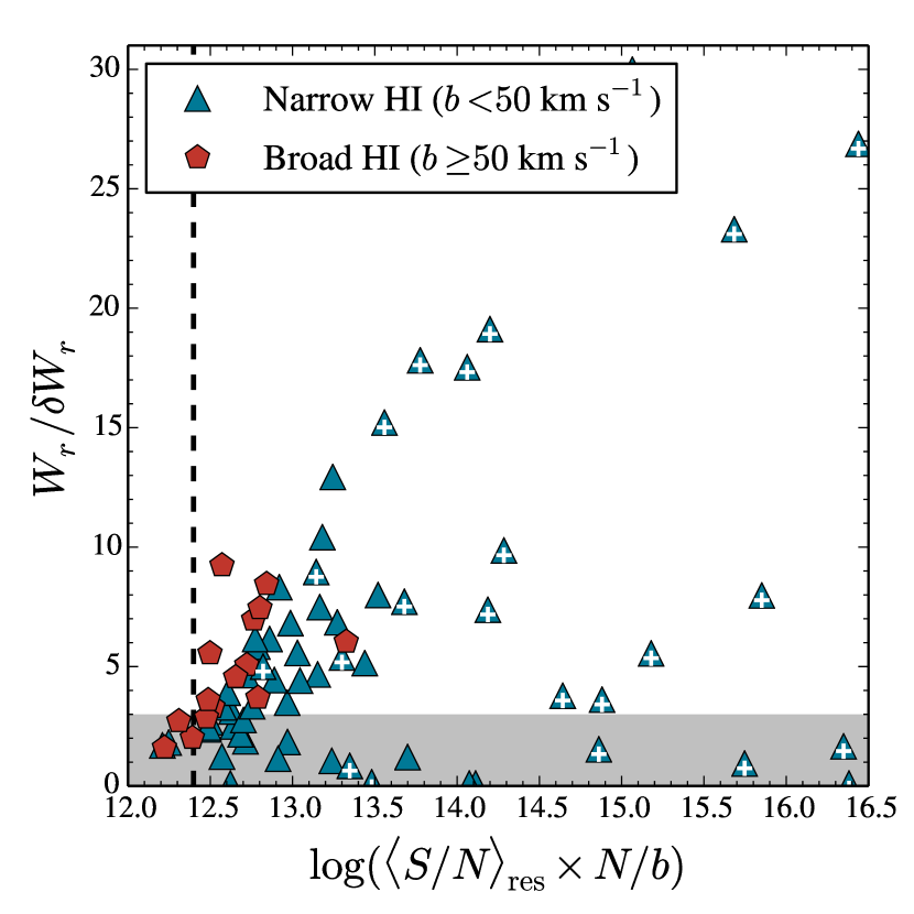
Figure 12: Comparison between two different methods for estimating the significance level of absorption line features. The $x$-axis corresponds to the $\log(\langle S/N\rangle_{\rm res}\times\ N/b)$ values proposed by Richter et al. (2006) (at least for broad H i lines) where $N$ is in units of cm^-2 and $b$ in , while the $y$-axis corresponds to our $W_{r}/\delta W_{r}$ (see Section 4.3). Blue triangles correspond to narrow H i absorption components ($b<50$ ), while red pentagons correspond to broad H i absorption components ($b\geq 50$ ), both found across the full Q1410 spectrum. White crosses mark components having multiple transitions, hence reliable (label ‘a’; see Section 4.5). The grey shaded area correspond to values $W_{r}/\delta W_{r}<3$, while the vertical dashed line correspond to a value of $\langle S/N\rangle_{\rm res}\times\ N/b=2.5\times 10^{12}$ cm^-2 $($km s${}^{-1})^{-1}$. See Appendix B for further details.

Here we compare two methods for estimating the significance level of absorption features, namely our $W_{\rm r}/\delta W_{\rm r}$ criterion (see Section 4.3) and $\langle S/R\rangle_{\rm res}\times N/b$ proposed by Richter et al. (2006) for broad H i absorption systems. The motivation for the later being that what matters to confidently detect a broad absorption line is both S/N and the optical depth at the line centres, $\tau_{0}\propto N/b$, and so it will not be appropriate to use the commonly adopted formalism based on a minimum equivalent width threshold for unresolved lines.

Figure 12 shows a comparison between these two quantities $\langle S/R\rangle_{\rm res}\times N/b$ in the $x$-axis and $W_{\rm r}/\delta W_{\rm r}$ in the $y$-axis), for our sample of H i absorption lines. Blue triangles correspond to H i  absorption components with $b<50$ (narrow), while red pentagons correspond to H i absorption components with $b\geq 50$ (broad) over the full Q1410 spectrum. White crosses mark components having multiple transitions, which we always account as reliable (label ‘a’; see Section 4.5). The grey shaded area corresponds to values $W_{\rm r}/\delta W_{\rm r}<3$.

Restricting ourselves to broad H i lines (red pentagons in Figure 12), we see a clear correlation between these two criteria. The dashed vertical line in Figure 12 corresponds to a value of $\langle S/R\rangle_{\rm res}\times N/b\geq 2.5\times 10^{12}$  cm^-2 $($km s${}^{-1})^{-1}$ for our COS data, which is needed to make both approaches roughly consistent with each other for broad H i lines. Such a value is similar to the one reported by Richter et al. (2006), $\langle S/R\rangle_{\rm res}\times N/b\geq 3\times 10^{12}$  cm^-2 $($km s${}^{-1})^{-1}$ in their STIS data.

For narrow H i lines (blue triangles in Figure 12) however, no clear correlation is present between these two methods, where several components having $W_{\rm r}/\delta W_{\rm r}<3$, can still have large values of $\langle S/R\rangle_{\rm res}\times N/b$. We note that many of the large $\langle S/R\rangle_{\rm res}\times N/b$ components are reliable (white crosses in Figure 12), but many others at the lower end are not. In terms of $W_{\rm r}/\delta W_{\rm r}$, we see that some reliable lines fall below the limit of $W_{\rm r}/\delta W_{\rm r}<3$. This is due to the fact that our adopted conservative method for estimating $W_{\rm r}$ (see Section 4.3) will give unrealistically large uncertainties, $\delta W_{\rm r}$, for unconstrained or saturated components. Indeed the vast majority of reliable components with $W_{\rm r}/\delta W_{\rm r}<3$ are saturated lines for which the column densities are not well determined.

Our proposed significance estimation based on $W_{\rm r}/\delta W_{\rm r}$ (and the presence of multiple transitions in a given component; see Section 4.5) can be straightforwardly applicable to any absorption line irrespective of its Doppler parameter and ionic transition. Therefore it has the advantage of allowing an homogeneous analysis.

Appendix C Estimation of redshift paths and absorption distances

We estimate $\Delta z(\Delta d,\Delta v,W_{\rm r}^{\rm min})$ and $\Delta X(\Delta d,\Delta v,W_{\rm r}^{\rm min})$ as follows. First, for a given transition we just considered regions in the Q1410 spectrum probing rest-frame velocity differences within $\Delta v$ from any cluster-pair within $\Delta d$ from the Q1410 sightline, and within our redshift range of $0.1\leq z\leq 0.5$. We also masked out regions with fluxes below $50\%$ the value of the continuum fit, to account for the fact that we are usually biased against finding absorption systems on top of strong absorption lines. We also masked out regions within $\pm 200$from strong Galactic absorption could exist, namely C ii $\lambda 1334.53$, N v $\lambda\lambda 1238.82,1242.80$, O i $\lambda 1302.17$, O i* $\lambda 1304.86$, O i** $\lambda 1306.03$, Si ii $\lambda\lambda 1260.42,1304.37$, P iii $\lambda 1334.81$, S ii $\lambda\lambda 1253.81,1259.52$ and Fe ii $\lambda 1260.53$. We then calculated the minimum rest-frame equivalent width to observe a transition at rest-frame wavelenght, $\lambda_{0}$, along the spectrum as,

$$W_{\rm r,\lambda_{0}}^{\rm min}=3\frac{\lambda_{0}/R}{\langle S/R\rangle}$$ (7)

where $R$ is the resolution of the spectrograph (taken to be $R=20\,000$), and $\langle S/R\rangle$ is the signal-to-noise ratio of the spectrum smoothed over $2$ pixels using a box-car filter (i.e. $\sim 1$ resolution element). We then identified chunks of the spectrum satisfying the criteria of $W_{\rm r,\lambda_{0}}^{\rm min}\geq W_{\rm r}^{\rm min}$, and recorded each corresponding minimum and maximum redshift, $z^{\rm min}_{i}(\Delta d,\Delta v,W_{\rm r}^{\rm min})$ and $z^{\rm max}_{i}(\Delta d,\Delta v,W_{\rm r}^{\rm min})$, in the $i$-th spectral chunk. We then computed the redshift path as,

$$\Delta z(\Delta d,\Delta v,W_{\rm r}^{\rm min})=\sum_{i}(z^{\rm max}_{i}-z^{\rm min}_{i})\ \rm{,}$$ (8)

and the absorption distance as,

$$\Delta X(\Delta d,\Delta v,W_{\rm r}^{\rm min})=\sum_{i}\int_{z^{\rm min}_{i}}^{z^{\rm max}_{i}}\frac{(1+z)^{2}}{\sqrt{\Omega_{\rm m}(1+z)^{3}+\Omega_{\rm\Lambda}}}{\rm d}z\ \rm{,}$$ (9)

conforming our adopted cosmology.

Appendix D Equivalent widths distributions

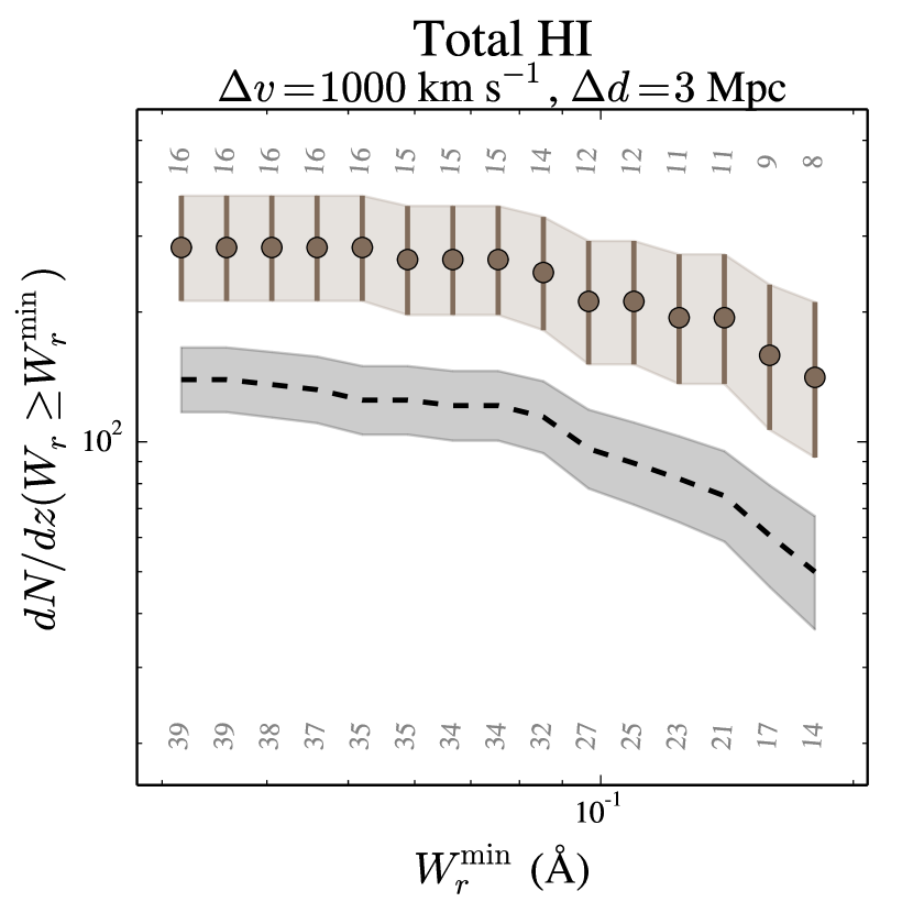
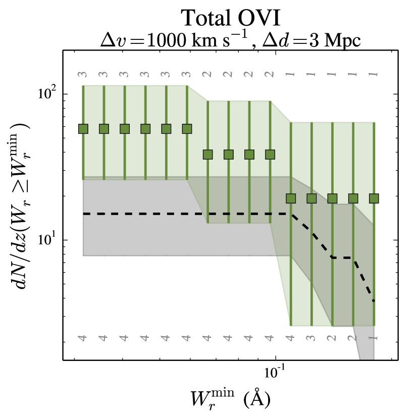
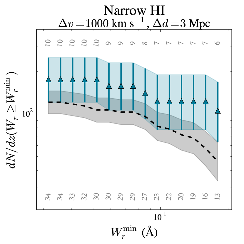
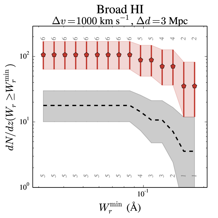
Figure 13: Redshift number density of our different samples of absorption lines associated to our cluster-pairs (i.e. using our fiducial values of $\Delta d=3$ Mpc and $\Delta v=1000$), as a function of minimum rest-frame equivalent width $W_{r}^{\rm min}$. The top panels show the results for our total H i (left panel) and O vi (right panel), while the bottom panels show the results for narrow (NLA; $b<50$) and broad (BLA; $b\geq 50$) H i, using the same colour/symbol convention as in Figure 6 to 10. Note that bins are not independent from each other, as emphasized by the light coloured areas. The field distributions estimated from our Q1410 sightline are represented by the dashed line with its $\pm 1\sigma$ uncertainty represented by the darker grey region. The total number of lines per bin are given in grey numbers on top and bottom of each panel, for our cluster-pairs and field samples respectively. See Appendix D for further details.

In this section we explore how do the equivalent widths distributions from our sample of lines associated with cluster-pairs (i.e. adopting our fiducial values of $\Delta d=3$ Mpc and $\Delta v=1000$), compare to those of the field expectation.

Figure 13 shows the redshift number density, $dN/dz$, of our different samples of absorption lines as a function of minimum rest-frame equivalent width, $W_{\rm r}^{\rm min}$, associated with our cluster-pairs: total H i (top left panel; brown circles), O vi (top right panel; green squares), narrow H i (bottom left panel; blue triangles) and broad H i (bottom right panel; red pentagons). The field distributions estimated from our Q1410 sightline are represented by the dashed line with its $\pm 1\sigma$ uncertainty represented by the darker grey region. Such field estimation comes from lines not being in the sample associated with cluster pairs, and its redshift path is estimated by excluding that of cluster-pairs too.

We observe that the equivalent widths distributions are not remarkably different between lines associated with cluster-pairs and the field expectation, and hence the relative excess in $dN/dz$ seems to remain somewhat constant as a function of $W_{\rm r}^{\rm min}$. The Kolmogorov-Smirnov test (K-S) for the unbinned $W_{\rm r}$ distributions between our cluster-pair and field samples give no statistically significant differences between them, but we note any possible real difference would be hard to detect because the samples are quite small ($\lesssim 10$).

We conclude that, in terms of equivalent widths, our cluster-pair absorption line samples and the field expectations are not significantly different, at least from what can be obtained in our limited sample.

Appendix E Q1410 HST/COS spectrum

Figure 14 shows the reduced Q1410 spectrum (black line), its corresponding uncertainty (green lines) and our adopted pseudo-continuum fit (blue dotted line). The figure also shows our Voigt profile fit solutions and residuals (red lines and grey dots respectively; see Section 4.2), and their corresponding IDs and reliability labels (see Section 4.5 and Table 4).

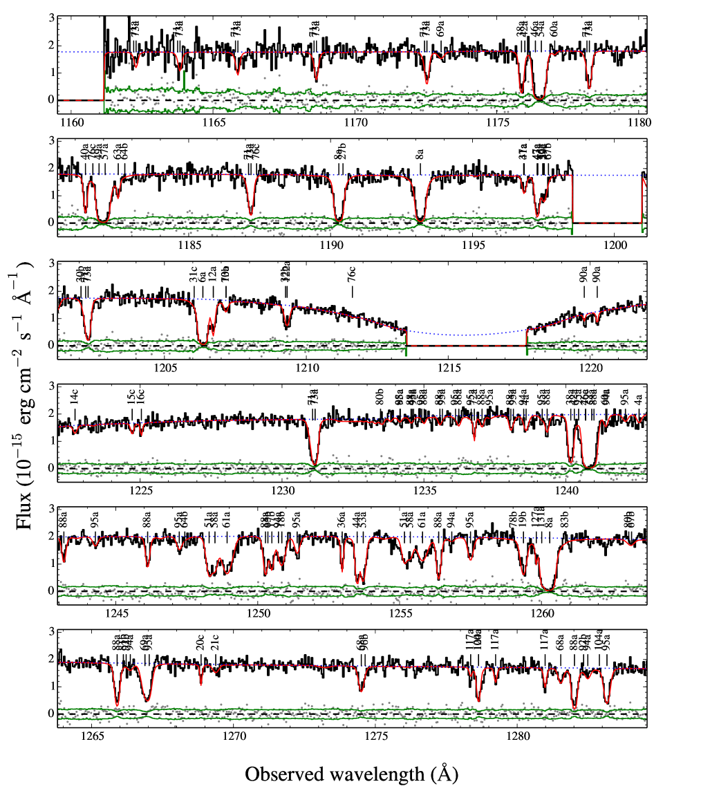
Figure 14: Observed HST/COS FUV spectrum of QSO Q1410 (black line), and its respective uncertainty (green lines). The red line correspond to our fit of the spectrum (see Section 4.2), while the blue dotted line corresponds to the assumed unabsorbed pseudo-continuum (i.e. including broad emission lines and the Milky Way’s DLA; see Section 2.2). Vertical tick lines indicate individual absorption lines, where the numbers correspond to the IDs given in Table 4 and the letters indicate their reliability (see Section 4.5). Grey points show the difference between our model and the observed data. We see that distribution of these residuals are consistent with the uncertainty of the data.

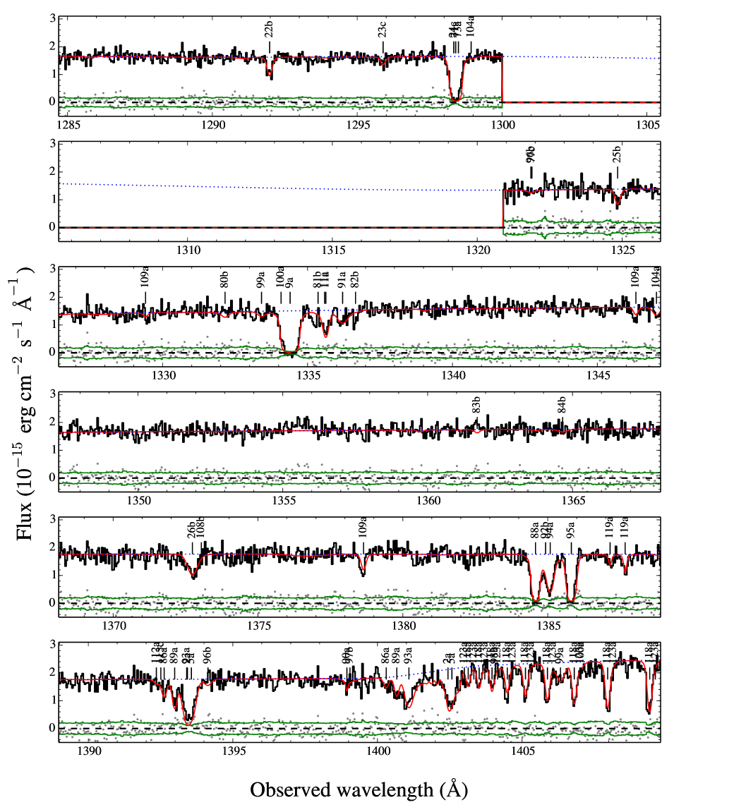
Figure 15: continued

Figure 16: continued

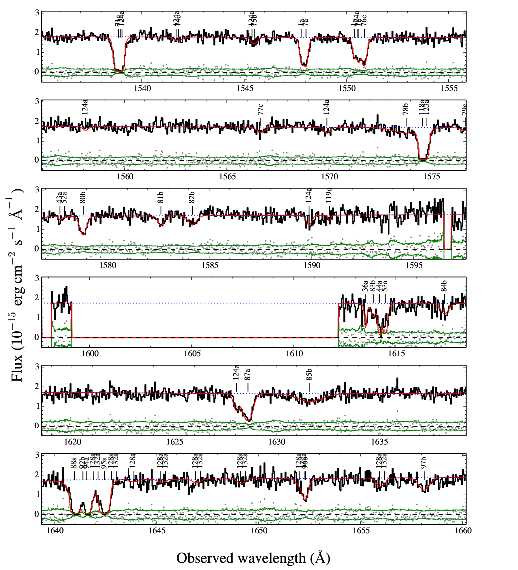
Figure 17: continued

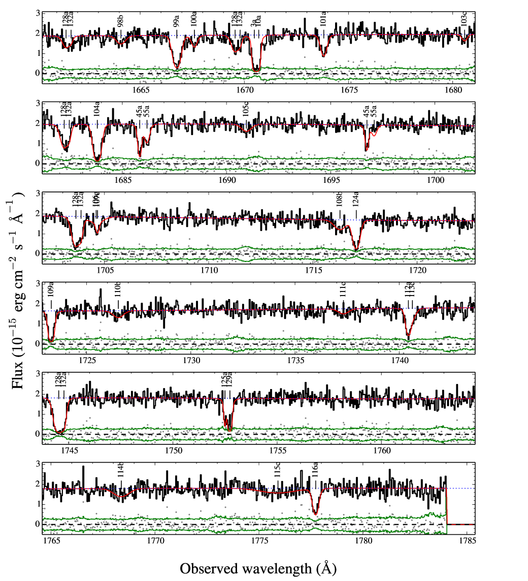
Figure 18: continued

Appendix F Visual association of absorption line systems with cluster-pairs

Figure 19 shows an schematic view of the association between H i and O vi absorption line systems and our known cluster-pairs obtained from the redMaPPer catalog (see Section 3). These plots are for illustrative purposes only; in cases with multiple grouped cluster-pairs (see Section 3.3) the chosen redshifts for defining rest-frames are arbitrary, but such choice is not used in our scientific analyses.

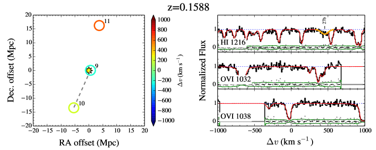
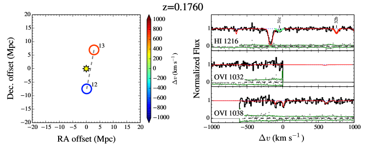
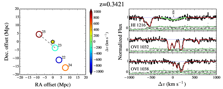
Figure 19: Schematic view of the clusters and cluster-pairs around the Q1410 sightline at different given redshifts (see top label in subpanels). The left panels correspond to the projected in the sky distribution of clusters (circles) and cluster-pairs (dashed lines) around the Q1410 sightline (yellow star) in co-moving  Mpc. Numbers close to the circles correspond to the cluster IDs as given in Table 2. The colour of the circles correspond to the rest-frame velocity difference of each cluster with respect to the given redshift, according to the colour bar scale on the right of the panel. The right panels correspond to portions of the normalized Q1410 HST/COS spectrum within a rest-frame velocity window of $\pm 1000$from the given redshift, for the H i   transition (top) and the O vi $\lambda\lambda 1032,1038$ Åtransitions (middle and bottom, respectively). The spectrum itself is represented by the black lines and the uncertainty is represented by the green line. Our fits to associated absorption line systems are represented by the thick coloured lines according to the colour bar scale on the left of the panel, while the fits for unassociated absorption line systems (i.e. at different redshifts) are represented by the red lines. Absorption line ID and reliability flags are given for associated absorption line systems.

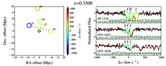
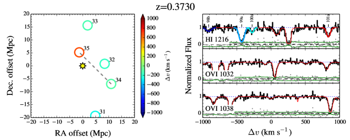
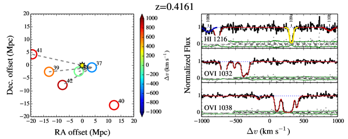
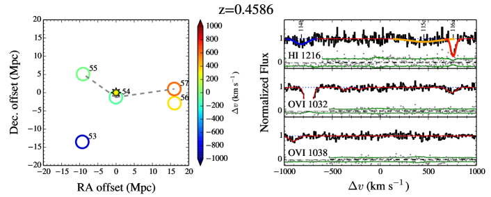
Figure 20: continued

Appendix G Summary tables for our incidence measurements

Tables 7 to 10 show a summary of our main $dN/dz$ and $dN/dX$ calculations for our different samples of absorption lines.

Table 7: Summary of relevant quantities for our sample of total H i absorption lines.

$\Delta d$	$\Delta v$	$W_{r}^{\rm min}$	$\Delta z$	$\Delta X$	$N$	$\frac{dN}{dz}$	$\frac{dN}{dX}$	$\frac{dN}{dz}|_{\rm field}$	$\frac{dN}{dX}|_{\rm field}$	$\frac{dN}{dz}/\frac{dN}{dz}|_{\rm field}$	$\frac{dN}{dX}/\frac{dN}{dX}|_{\rm field}$
( Mpc)	()	(Å)
(1)	(2)	(3)	(4)	(5)	(6)	(7)	(8)	(9)	(10)	(11)	(12)
3.0	500	0.04	0.03	0.05	11	$358^{+144}_{-107}$	$238^{+96}_{-71}$	$123^{+26}_{-23}$	$87^{+18}_{-16}$	$2.9^{+1.2}_{-0.9}$	$2.7^{+1.1}_{-0.9}$
3.0	630	0.04	0.04	0.06	11	$293^{+118}_{-87}$	$195^{+78}_{-58}$	$123^{+26}_{-23}$	$87^{+18}_{-16}$	$2.4^{+1.0}_{-0.7}$	$2.2^{+0.9}_{-0.7}$
3.0	794	0.04	0.05	0.07	14	$305^{+105}_{-81}$	$203^{+70}_{-54}$	$123^{+26}_{-23}$	$87^{+18}_{-16}$	$2.5^{+0.9}_{-0.7}$	$2.3^{+0.8}_{-0.7}$
3.0	1000	0.04	0.06	0.08	16	$287^{+91}_{-71}$	$191^{+61}_{-47}$	$123^{+26}_{-23}$	$87^{+18}_{-16}$	$2.3^{+0.8}_{-0.6}$	$2.2^{+0.7}_{-0.6}$
3.0	1313	0.04	0.07	0.11	17	$237^{+73}_{-57}$	$159^{+49}_{-38}$	$123^{+26}_{-23}$	$87^{+18}_{-16}$	$1.9^{+0.6}_{-0.5}$	$1.8^{+0.6}_{-0.5}$
3.0	1724	0.04	0.09	0.13	17	$188^{+58}_{-45}$	$126^{+39}_{-30}$	$123^{+26}_{-23}$	$87^{+18}_{-16}$	$1.5^{+0.5}_{-0.4}$	$1.5^{+0.5}_{-0.4}$
3.0	2264	0.04	0.12	0.17	18	$156^{+46}_{-37}$	$105^{+31}_{-25}$	$123^{+26}_{-23}$	$87^{+18}_{-16}$	$1.3^{+0.4}_{-0.3}$	$1.2^{+0.4}_{-0.3}$
3.0	2972	0.04	0.14	0.21	21	$151^{+41}_{-33}$	$101^{+27}_{-22}$	$123^{+26}_{-23}$	$87^{+18}_{-16}$	$1.2^{+0.4}_{-0.3}$	$1.2^{+0.3}_{-0.3}$
3.0	3903	0.04	0.16	0.24	25	$152^{+37}_{-30}$	$102^{+25}_{-20}$	$123^{+26}_{-23}$	$87^{+18}_{-16}$	$1.2^{+0.3}_{-0.3}$	$1.2^{+0.3}_{-0.3}$
3.0	5125	0.04	0.18	0.27	26	$143^{+34}_{-28}$	$97^{+23}_{-19}$	$123^{+26}_{-23}$	$87^{+18}_{-16}$	$1.2^{+0.3}_{-0.3}$	$1.1^{+0.3}_{-0.2}$
3.0	6729	0.04	0.19	0.28	26	$134^{+32}_{-26}$	$91^{+22}_{-18}$	$123^{+26}_{-23}$	$87^{+18}_{-16}$	$1.1^{+0.3}_{-0.2}$	$1.1^{+0.3}_{-0.2}$
3.0	8835	0.04	0.22	0.32	32	$147^{+31}_{-26}$	$101^{+21}_{-18}$	$123^{+26}_{-23}$	$87^{+18}_{-16}$	$1.2^{+0.3}_{-0.2}$	$1.2^{+0.3}_{-0.2}$
3.0	11601	0.04	0.25	0.36	38	$151^{+29}_{-24}$	$105^{+20}_{-17}$	$123^{+26}_{-23}$	$87^{+18}_{-16}$	$1.2^{+0.3}_{-0.2}$	$1.2^{+0.3}_{-0.2}$
3.0	15232	0.04	0.30	0.42	43	$146^{+26}_{-22}$	$103^{+18}_{-16}$	$123^{+26}_{-23}$	$87^{+18}_{-16}$	$1.2^{+0.2}_{-0.2}$	$1.2^{+0.2}_{-0.2}$
3.0	20000	0.04	0.33	0.47	48	$145^{+24}_{-21}$	$103^{+17}_{-15}$	$123^{+26}_{-23}$	$87^{+18}_{-16}$	$1.2^{+0.2}_{-0.2}$	$1.2^{+0.2}_{-0.2}$
1.0	1000	0.04	0.01	0.02	3	$203^{+199}_{-112}$	$140^{+137}_{-77}$	$123^{+26}_{-23}$	$87^{+18}_{-16}$	$1.6^{+1.6}_{-0.9}$	$1.6^{+1.6}_{-0.9}$
1.4	1000	0.04	0.03	0.04	6	$231^{+139}_{-92}$	$150^{+90}_{-60}$	$123^{+26}_{-23}$	$87^{+18}_{-16}$	$1.9^{+1.1}_{-0.8}$	$1.7^{+1.1}_{-0.7}$
2.1	1000	0.04	0.04	0.06	8	$184^{+91}_{-64}$	$124^{+61}_{-43}$	$123^{+26}_{-23}$	$87^{+18}_{-16}$	$1.5^{+0.8}_{-0.5}$	$1.4^{+0.7}_{-0.5}$
3.0	1000	0.04	0.06	0.08	16	$287^{+91}_{-71}$	$191^{+61}_{-47}$	$123^{+26}_{-23}$	$87^{+18}_{-16}$	$2.3^{+0.8}_{-0.6}$	$2.2^{+0.7}_{-0.6}$
4.1	1000	0.04	0.06	0.09	16	$280^{+89}_{-69}$	$187^{+59}_{-46}$	$123^{+26}_{-23}$	$87^{+18}_{-16}$	$2.3^{+0.8}_{-0.6}$	$2.2^{+0.7}_{-0.6}$
5.7	1000	0.04	0.06	0.09	16	$279^{+89}_{-69}$	$186^{+59}_{-46}$	$123^{+26}_{-23}$	$87^{+18}_{-16}$	$2.3^{+0.8}_{-0.6}$	$2.1^{+0.7}_{-0.6}$
7.8	1000	0.04	0.07	0.10	16	$242^{+77}_{-60}$	$164^{+52}_{-41}$	$123^{+26}_{-23}$	$87^{+18}_{-16}$	$2.0^{+0.7}_{-0.5}$	$1.9^{+0.6}_{-0.5}$
10.7	1000	0.04	0.08	0.12	17	$218^{+67}_{-53}$	$147^{+45}_{-35}$	$123^{+26}_{-23}$	$87^{+18}_{-16}$	$1.8^{+0.6}_{-0.5}$	$1.7^{+0.5}_{-0.4}$
14.8	1000	0.04	0.09	0.14	19	$205^{+59}_{-47}$	$140^{+40}_{-32}$	$123^{+26}_{-23}$	$87^{+18}_{-16}$	$1.7^{+0.5}_{-0.4}$	$1.6^{+0.5}_{-0.4}$
20.3	1000	0.04	0.11	0.16	21	$193^{+52}_{-42}$	$132^{+36}_{-29}$	$123^{+26}_{-23}$	$87^{+18}_{-16}$	$1.6^{+0.5}_{-0.4}$	$1.5^{+0.4}_{-0.4}$
27.9	1000	0.04	0.12	0.17	23	$195^{+50}_{-40}$	$133^{+34}_{-28}$	$123^{+26}_{-23}$	$87^{+18}_{-16}$	$1.6^{+0.4}_{-0.4}$	$1.5^{+0.4}_{-0.4}$
38.4	1000	0.04	0.15	0.22	27	$180^{+42}_{-35}$	$124^{+29}_{-24}$	$123^{+26}_{-23}$	$87^{+18}_{-16}$	$1.5^{+0.4}_{-0.3}$	$1.4^{+0.4}_{-0.3}$
52.9	1000	0.04	0.17	0.24	27	$160^{+37}_{-31}$	$111^{+26}_{-21}$	$123^{+26}_{-23}$	$87^{+18}_{-16}$	$1.3^{+0.3}_{-0.3}$	$1.3^{+0.3}_{-0.3}$
72.7	1000	0.04	0.19	0.28	29	$150^{+33}_{-28}$	$105^{+23}_{-19}$	$123^{+26}_{-23}$	$87^{+18}_{-16}$	$1.2^{+0.3}_{-0.3}$	$1.2^{+0.3}_{-0.3}$
100.0	1000	0.04	0.24	0.35	39	$160^{+30}_{-25}$	$113^{+21}_{-18}$	$123^{+26}_{-23}$	$87^{+18}_{-16}$	$1.3^{+0.3}_{-0.2}$	$1.3^{+0.3}_{-0.2}$
3.0	1000	0.03	0.06	0.09	16	$282^{+90}_{-70}$	$188^{+60}_{-47}$	$139^{+26}_{-22}$	$100^{+19}_{-16}$	$2.0^{+0.7}_{-0.6}$	$1.9^{+0.7}_{-0.6}$
3.0	1000	0.04	0.06	0.09	16	$282^{+90}_{-70}$	$188^{+60}_{-47}$	$139^{+26}_{-22}$	$100^{+19}_{-16}$	$2.0^{+0.7}_{-0.6}$	$1.9^{+0.7}_{-0.6}$
3.0	1000	0.04	0.06	0.09	16	$282^{+90}_{-70}$	$188^{+60}_{-47}$	$136^{+26}_{-22}$	$97^{+18}_{-16}$	$2.1^{+0.8}_{-0.6}$	$1.9^{+0.7}_{-0.6}$
3.0	1000	0.05	0.06	0.09	16	$282^{+90}_{-70}$	$188^{+60}_{-47}$	$132^{+26}_{-22}$	$94^{+18}_{-15}$	$2.1^{+0.8}_{-0.7}$	$2.0^{+0.7}_{-0.6}$
3.0	1000	0.05	0.06	0.09	16	$282^{+90}_{-70}$	$188^{+60}_{-47}$	$125^{+25}_{-21}$	$89^{+18}_{-15}$	$2.3^{+0.8}_{-0.7}$	$2.1^{+0.8}_{-0.7}$
3.0	1000	0.06	0.06	0.09	15	$265^{+88}_{-68}$	$176^{+58}_{-45}$	$125^{+25}_{-21}$	$89^{+18}_{-15}$	$2.1^{+0.8}_{-0.7}$	$2.0^{+0.7}_{-0.6}$
3.0	1000	0.07	0.06	0.09	15	$265^{+88}_{-68}$	$176^{+58}_{-45}$	$121^{+25}_{-21}$	$87^{+18}_{-15}$	$2.2^{+0.8}_{-0.7}$	$2.0^{+0.8}_{-0.6}$
3.0	1000	0.08	0.06	0.09	15	$265^{+88}_{-68}$	$176^{+58}_{-45}$	$121^{+25}_{-21}$	$87^{+18}_{-15}$	$2.2^{+0.8}_{-0.7}$	$2.0^{+0.8}_{-0.6}$
3.0	1000	0.09	0.06	0.09	14	$247^{+85}_{-65}$	$165^{+57}_{-44}$	$114^{+24}_{-20}$	$82^{+17}_{-14}$	$2.2^{+0.9}_{-0.7}$	$2.0^{+0.8}_{-0.7}$
3.0	1000	0.10	0.06	0.09	12	$212^{+81}_{-60}$	$141^{+54}_{-40}$	$96^{+22}_{-18}$	$69^{+16}_{-13}$	$2.2^{+1.0}_{-0.8}$	$2.0^{+0.9}_{-0.7}$
3.0	1000	0.11	0.06	0.09	12	$212^{+81}_{-60}$	$141^{+54}_{-40}$	$89^{+22}_{-18}$	$64^{+15}_{-13}$	$2.4^{+1.0}_{-0.9}$	$2.2^{+1.0}_{-0.8}$
3.0	1000	0.12	0.06	0.09	11	$194^{+78}_{-58}$	$129^{+52}_{-39}$	$82^{+21}_{-17}$	$59^{+15}_{-12}$	$2.4^{+1.1}_{-0.9}$	$2.2^{+1.0}_{-0.8}$
3.0	1000	0.14	0.06	0.09	11	$194^{+78}_{-58}$	$129^{+52}_{-39}$	$75^{+20}_{-16}$	$54^{+14}_{-12}$	$2.6^{+1.2}_{-1.0}$	$2.4^{+1.1}_{-0.9}$
3.0	1000	0.16	0.06	0.09	9	$159^{+73}_{-52}$	$106^{+48}_{-35}$	$61^{+19}_{-15}$	$43^{+13}_{-10}$	$2.6^{+1.4}_{-1.1}$	$2.4^{+1.3}_{-1.0}$
3.0	1000	0.18	0.06	0.09	8	$141^{+70}_{-49}$	$94^{+47}_{-33}$	$50^{+17}_{-13}$	$36^{+12}_{-9}$	$2.8^{+1.6}_{-1.3}$	$2.6^{+1.5}_{-1.2}$

(1) Maximum transverse separation between cluster-pair axes and the Q1410 sightline (see Section 5.1). (2) Maximum velocity difference to any cluster-pair within $\Delta d$ from the Q1410 sightline (see Section 5.1). (3) Minimum rest-frame equivalent width (see Section 5.1). (4) Redshift path (see Section 5.1 and Appendix C). (5) Absorption distance (see Appendix C). (6) Total number of absorption components having $W_{\rm r}\geq W_{\rm r}^{\rm min}$ within $\Delta d$ and $\Delta v$ from cluster-pairs (see Section 5.1). (7) Redshift number density associated to absorption components having $W_{\rm r}\geq W_{\rm r}^{\rm min}$ within $\Delta d$ and $\Delta v$ from cluster-pairs (see Section 5.1). (8) Absorption distance number density to absorption components having $W_{\rm r}\geq W_{\rm r}^{\rm min}$ within $\Delta d$ and $\Delta v$ from cluster-pairs (analogous to $dN/dz$ but see also Appendix C) (9) Field expectation for the redshift number density (see Section 5.2). (10) Field expectation for the absorption distance number density (see Section 5.2). (11) Excess of the measured redshift number density compared to the field expectation (see Section 6.2). (12) Excess of the measured absorption distance number density compared to the field expectation (see Section 6.2).

Table 8: Summary of relevant quantities for our sample of total O vi absorption lines.

$\Delta d$	$\Delta v$	$W_{r}^{\rm min}$	$\Delta z$	$\Delta X$	$N$	$\frac{dN}{dz}$	$\frac{dN}{dX}$	$\frac{dN}{dz}|_{\rm field}$	$\frac{dN}{dX}|_{\rm field}$	$\frac{dN}{dz}/\frac{dN}{dz}|_{\rm field}$	$\frac{dN}{dX}/\frac{dN}{dX}|_{\rm field}$
( Mpc)	()	(Å)
(1)	(2)	(3)	(4)	(5)	(6)	(7)	(8)	(9)	(10)	(11)	(12)
3.0	500	0.06	0.03	0.05	3	$100^{+98}_{-55}$	$66^{+64}_{-36}$	$14^{+12}_{-8}$	$10^{+8}_{-6}$	$7.1^{+7.4}_{-4.7}$	$6.9^{+7.2}_{-4.5}$
3.0	630	0.06	0.04	0.06	3	$82^{+80}_{-45}$	$54^{+53}_{-30}$	$14^{+12}_{-8}$	$10^{+8}_{-6}$	$5.8^{+6.1}_{-3.8}$	$5.6^{+5.9}_{-3.7}$
3.0	794	0.06	0.04	0.07	3	$70^{+69}_{-39}$	$46^{+45}_{-26}$	$14^{+12}_{-8}$	$10^{+8}_{-6}$	$5.0^{+5.2}_{-3.3}$	$4.8^{+5.0}_{-3.2}$
3.0	1000	0.06	0.05	0.08	3	$58^{+57}_{-32}$	$38^{+37}_{-21}$	$14^{+12}_{-8}$	$10^{+8}_{-6}$	$4.1^{+4.3}_{-2.7}$	$4.0^{+4.2}_{-2.6}$
3.0	1313	0.06	0.07	0.10	3	$45^{+45}_{-25}$	$30^{+29}_{-17}$	$14^{+12}_{-8}$	$10^{+8}_{-6}$	$3.2^{+3.4}_{-2.1}$	$3.1^{+3.3}_{-2.1}$
3.0	1724	0.06	0.09	0.13	3	$35^{+34}_{-19}$	$23^{+23}_{-13}$	$14^{+12}_{-8}$	$10^{+8}_{-6}$	$2.5^{+2.6}_{-1.6}$	$2.4^{+2.5}_{-1.6}$
3.0	2264	0.06	0.11	0.17	3	$27^{+26}_{-15}$	$18^{+17}_{-10}$	$14^{+12}_{-8}$	$10^{+8}_{-6}$	$1.9^{+2.0}_{-1.3}$	$1.9^{+1.9}_{-1.2}$
3.0	2972	0.06	0.14	0.21	3	$22^{+21}_{-12}$	$14^{+14}_{-8}$	$14^{+12}_{-8}$	$10^{+8}_{-6}$	$1.5^{+1.6}_{-1.0}$	$1.5^{+1.6}_{-1.0}$
3.0	3903	0.06	0.17	0.26	3	$17^{+17}_{-10}$	$12^{+11}_{-6}$	$14^{+12}_{-8}$	$10^{+8}_{-6}$	$1.2^{+1.3}_{-0.8}$	$1.2^{+1.3}_{-0.8}$
3.0	5125	0.06	0.20	0.30	3	$15^{+15}_{-8}$	$10^{+10}_{-5}$	$14^{+12}_{-8}$	$10^{+8}_{-6}$	$1.1^{+1.1}_{-0.7}$	$1.0^{+1.1}_{-0.7}$
3.0	6729	0.06	0.23	0.34	3	$13^{+13}_{-7}$	$9^{+9}_{-5}$	$14^{+12}_{-8}$	$10^{+8}_{-6}$	$0.9^{+1.0}_{-0.6}$	$0.9^{+1.0}_{-0.6}$
3.0	8835	0.06	0.25	0.38	6	$24^{+14}_{-9}$	$16^{+9}_{-6}$	$14^{+12}_{-8}$	$10^{+8}_{-6}$	$1.7^{+1.2}_{-0.9}$	$1.7^{+1.2}_{-0.9}$
3.0	11601	0.06	0.27	0.40	6	$22^{+13}_{-9}$	$15^{+9}_{-6}$	$14^{+12}_{-8}$	$10^{+8}_{-6}$	$1.6^{+1.1}_{-0.9}$	$1.6^{+1.1}_{-0.8}$
3.0	15232	0.06	0.29	0.44	7	$24^{+13}_{-9}$	$16^{+9}_{-6}$	$14^{+12}_{-8}$	$10^{+8}_{-6}$	$1.7^{+1.1}_{-0.9}$	$1.7^{+1.1}_{-0.9}$
3.0	20000	0.06	0.32	0.46	7	$22^{+12}_{-8}$	$15^{+8}_{-6}$	$14^{+12}_{-8}$	$10^{+8}_{-6}$	$1.6^{+1.0}_{-0.8}$	$1.6^{+1.0}_{-0.8}$
1.0	1000	0.06	0.01	0.02	0	$0^{+132}_{-0}$	$0^{+91}_{-0}$	$14^{+12}_{-8}$	$10^{+8}_{-6}$	$0.0^{+9.4}_{-0.0}$	$0.0^{+9.5}_{-0.0}$
1.4	1000	0.06	0.03	0.04	0	$0^{+73}_{-0}$	$0^{+47}_{-0}$	$14^{+12}_{-8}$	$10^{+8}_{-6}$	$0.0^{+5.2}_{-0.0}$	$0.0^{+4.9}_{-0.0}$
2.1	1000	0.06	0.04	0.06	0	$0^{+48}_{-0}$	$0^{+32}_{-0}$	$14^{+12}_{-8}$	$10^{+8}_{-6}$	$0.0^{+3.4}_{-0.0}$	$0.0^{+3.3}_{-0.0}$
3.0	1000	0.06	0.05	0.08	3	$58^{+57}_{-32}$	$38^{+37}_{-21}$	$14^{+12}_{-8}$	$10^{+8}_{-6}$	$4.1^{+4.3}_{-2.7}$	$4.0^{+4.2}_{-2.6}$
4.1	1000	0.06	0.05	0.08	3	$56^{+55}_{-31}$	$37^{+36}_{-20}$	$14^{+12}_{-8}$	$10^{+8}_{-6}$	$4.0^{+4.2}_{-2.6}$	$3.9^{+4.0}_{-2.6}$
5.7	1000	0.06	0.05	0.08	3	$56^{+55}_{-31}$	$37^{+36}_{-20}$	$14^{+12}_{-8}$	$10^{+8}_{-6}$	$4.0^{+4.1}_{-2.6}$	$3.8^{+4.0}_{-2.5}$
7.8	1000	0.06	0.06	0.09	3	$48^{+47}_{-27}$	$32^{+32}_{-18}$	$14^{+12}_{-8}$	$10^{+8}_{-6}$	$3.4^{+3.6}_{-2.3}$	$3.4^{+3.5}_{-2.2}$
10.7	1000	0.06	0.07	0.11	3	$40^{+39}_{-22}$	$27^{+26}_{-15}$	$14^{+12}_{-8}$	$10^{+8}_{-6}$	$2.8^{+3.0}_{-1.9}$	$2.8^{+2.9}_{-1.8}$
14.8	1000	0.06	0.09	0.13	4	$45^{+36}_{-22}$	$31^{+24}_{-15}$	$14^{+12}_{-8}$	$10^{+8}_{-6}$	$3.2^{+2.8}_{-1.9}$	$3.2^{+2.8}_{-1.9}$
20.3	1000	0.06	0.10	0.15	4	$41^{+32}_{-20}$	$28^{+22}_{-13}$	$14^{+12}_{-8}$	$10^{+8}_{-6}$	$2.9^{+2.5}_{-1.8}$	$2.9^{+2.5}_{-1.7}$
27.9	1000	0.06	0.11	0.16	4	$37^{+29}_{-18}$	$25^{+20}_{-12}$	$14^{+12}_{-8}$	$10^{+8}_{-6}$	$2.6^{+2.3}_{-1.6}$	$2.6^{+2.3}_{-1.6}$
38.4	1000	0.06	0.13	0.20	4	$30^{+24}_{-14}$	$20^{+16}_{-10}$	$14^{+12}_{-8}$	$10^{+8}_{-6}$	$2.1^{+1.9}_{-1.3}$	$2.1^{+1.8}_{-1.3}$
52.9	1000	0.06	0.16	0.24	4	$25^{+20}_{-12}$	$17^{+13}_{-8}$	$14^{+12}_{-8}$	$10^{+8}_{-6}$	$1.8^{+1.5}_{-1.1}$	$1.7^{+1.5}_{-1.1}$
72.7	1000	0.06	0.19	0.28	4	$21^{+17}_{-10}$	$14^{+11}_{-7}$	$14^{+12}_{-8}$	$10^{+8}_{-6}$	$1.5^{+1.3}_{-0.9}$	$1.5^{+1.3}_{-0.9}$
100.0	1000	0.06	0.25	0.37	7	$28^{+15}_{-11}$	$19^{+10}_{-7}$	$14^{+12}_{-8}$	$10^{+8}_{-6}$	$2.0^{+1.3}_{-1.0}$	$2.0^{+1.3}_{-1.0}$
3.0	1000	0.03	0.05	0.08	3	$58^{+57}_{-32}$	$38^{+37}_{-21}$	$15^{+12}_{-7}$	$10^{+8}_{-5}$	$3.8^{+4.5}_{-3.2}$	$3.7^{+4.3}_{-3.1}$
3.0	1000	0.04	0.05	0.08	3	$58^{+57}_{-32}$	$38^{+37}_{-21}$	$15^{+12}_{-7}$	$10^{+8}_{-5}$	$3.8^{+4.5}_{-3.2}$	$3.7^{+4.3}_{-3.1}$
3.0	1000	0.04	0.05	0.08	3	$58^{+57}_{-32}$	$38^{+37}_{-21}$	$15^{+12}_{-7}$	$10^{+8}_{-5}$	$3.8^{+4.5}_{-3.2}$	$3.7^{+4.3}_{-3.1}$
3.0	1000	0.05	0.05	0.08	3	$58^{+57}_{-32}$	$38^{+37}_{-21}$	$15^{+12}_{-7}$	$10^{+8}_{-5}$	$3.8^{+4.5}_{-3.2}$	$3.7^{+4.3}_{-3.1}$
3.0	1000	0.05	0.05	0.08	3	$58^{+57}_{-32}$	$38^{+37}_{-21}$	$15^{+12}_{-7}$	$10^{+8}_{-5}$	$3.8^{+4.5}_{-3.2}$	$3.7^{+4.3}_{-3.1}$
3.0	1000	0.06	0.05	0.08	3	$58^{+57}_{-32}$	$38^{+37}_{-21}$	$15^{+12}_{-7}$	$10^{+8}_{-5}$	$3.8^{+4.5}_{-3.2}$	$3.7^{+4.3}_{-3.1}$
3.0	1000	0.07	0.05	0.08	2	$39^{+51}_{-25}$	$25^{+34}_{-17}$	$15^{+12}_{-7}$	$10^{+8}_{-5}$	$2.5^{+3.8}_{-2.3}$	$2.5^{+3.6}_{-2.3}$
3.0	1000	0.08	0.05	0.08	2	$39^{+51}_{-25}$	$25^{+34}_{-17}$	$15^{+12}_{-7}$	$10^{+8}_{-5}$	$2.5^{+3.8}_{-2.3}$	$2.5^{+3.6}_{-2.3}$
3.0	1000	0.09	0.05	0.08	2	$39^{+51}_{-25}$	$25^{+34}_{-17}$	$15^{+12}_{-7}$	$10^{+8}_{-5}$	$2.5^{+3.8}_{-2.3}$	$2.5^{+3.6}_{-2.3}$
3.0	1000	0.10	0.05	0.08	2	$39^{+51}_{-25}$	$25^{+34}_{-17}$	$15^{+12}_{-7}$	$10^{+8}_{-5}$	$2.5^{+3.8}_{-2.3}$	$2.5^{+3.6}_{-2.3}$
3.0	1000	0.11	0.05	0.08	1	$19^{+45}_{-17}$	$13^{+29}_{-11}$	$15^{+12}_{-7}$	$10^{+8}_{-5}$	$1.3^{+3.1}_{-1.3}$	$1.2^{+3.0}_{-1.2}$
3.0	1000	0.12	0.05	0.08	1	$19^{+45}_{-17}$	$13^{+29}_{-11}$	$11^{+11}_{-6}$	$8^{+8}_{-4}$	$1.7^{+4.2}_{-1.7}$	$1.6^{+4.0}_{-1.6}$
3.0	1000	0.14	0.05	0.08	1	$19^{+45}_{-17}$	$13^{+29}_{-11}$	$8^{+10}_{-5}$	$5^{+7}_{-3}$	$2.5^{+6.4}_{-2.5}$	$2.5^{+6.2}_{-2.5}$
3.0	1000	0.16	0.05	0.08	1	$19^{+45}_{-17}$	$13^{+29}_{-11}$	$8^{+10}_{-5}$	$5^{+7}_{-3}$	$2.5^{+6.4}_{-2.5}$	$2.5^{+6.2}_{-2.5}$
3.0	1000	0.18	0.05	0.08	1	$19^{+45}_{-17}$	$13^{+29}_{-11}$	$4^{+9}_{-3}$	$3^{+6}_{-2}$	$5.1^{+14.3}_{-5.1}$	$4.9^{+13.8}_{-4.9}$

(1) Maximum transverse separation between cluster-pair axes and the Q1410 sightline (see Section 5.1). (2) Maximum velocity difference to any cluster-pair within $\Delta d$ from the Q1410 sightline (see Section 5.1). (3) Minimum rest-frame equivalent width (see Section 5.1). (4) Redshift path (see Section 5.1 and Appendix C). (5) Absorption distance (see Appendix C). (6) Total number of absorption components having $W_{\rm r}\geq W_{\rm r}^{\rm min}$ within $\Delta d$ and $\Delta v$ from cluster-pairs (see Section 5.1). (7) Redshift number density associated to absorption components having $W_{\rm r}\geq W_{\rm r}^{\rm min}$ within $\Delta d$ and $\Delta v$ from cluster-pairs (see Section 5.1). (8) Absorption distance number density to absorption components having $W_{\rm r}\geq W_{\rm r}^{\rm min}$ within $\Delta d$ and $\Delta v$ from cluster-pairs (analogous to $dN/dz$ but see also Appendix C) (9) Field expectation for the redshift number density (see Section 5.2). (10) Field expectation for the absorption distance number density (see Section 5.2). (11) Excess of the measured redshift number density compared to the field expectation (see Section 6.2). (12) Excess of the measured absorption distance number density compared to the field expectation (see Section 6.2).

Table 9: Summary of relevant quantities for our sample of narrow H i ($b<50$) absorption lines.

$\Delta d$	$\Delta v$	$W_{r}^{\rm min}$	$\Delta z$	$\Delta X$	$N$	$\frac{dN}{dz}$	$\frac{dN}{dX}$	$\frac{dN}{dz}|_{\rm field}$	$\frac{dN}{dX}|_{\rm field}$	$\frac{dN}{dz}/\frac{dN}{dz}|_{\rm field}$	$\frac{dN}{dX}/\frac{dN}{dX}|_{\rm field}$
( Mpc)	()	(Å)
(1)	(2)	(3)	(4)	(5)	(6)	(7)	(8)	(9)	(10)	(11)	(12)
3.0	500	0.04	0.03	0.05	7	$228^{+123}_{-85}$	$151^{+82}_{-56}$	$106^{+23}_{-20}$	$75^{+16}_{-14}$	$2.2^{+1.2}_{-0.8}$	$2.0^{+1.1}_{-0.8}$
3.0	630	0.04	0.04	0.06	7	$186^{+101}_{-69}$	$124^{+67}_{-46}$	$106^{+23}_{-20}$	$75^{+16}_{-14}$	$1.8^{+1.0}_{-0.7}$	$1.7^{+0.9}_{-0.6}$
3.0	794	0.04	0.05	0.07	8	$174^{+86}_{-61}$	$116^{+57}_{-40}$	$106^{+23}_{-20}$	$75^{+16}_{-14}$	$1.6^{+0.8}_{-0.6}$	$1.6^{+0.8}_{-0.6}$
3.0	1000	0.04	0.06	0.08	10	$179^{+77}_{-56}$	$120^{+51}_{-37}$	$106^{+23}_{-20}$	$75^{+16}_{-14}$	$1.7^{+0.7}_{-0.6}$	$1.6^{+0.7}_{-0.5}$
3.0	1313	0.04	0.07	0.11	11	$154^{+62}_{-46}$	$103^{+41}_{-31}$	$106^{+23}_{-20}$	$75^{+16}_{-14}$	$1.5^{+0.6}_{-0.5}$	$1.4^{+0.6}_{-0.4}$
3.0	1724	0.04	0.09	0.13	11	$121^{+49}_{-36}$	$82^{+33}_{-24}$	$106^{+23}_{-20}$	$75^{+16}_{-14}$	$1.2^{+0.5}_{-0.4}$	$1.1^{+0.5}_{-0.3}$
3.0	2264	0.04	0.12	0.17	11	$95^{+38}_{-28}$	$64^{+26}_{-19}$	$106^{+23}_{-20}$	$75^{+16}_{-14}$	$0.9^{+0.4}_{-0.3}$	$0.9^{+0.4}_{-0.3}$
3.0	2972	0.04	0.14	0.21	14	$101^{+35}_{-27}$	$68^{+23}_{-18}$	$106^{+23}_{-20}$	$75^{+16}_{-14}$	$1.0^{+0.3}_{-0.3}$	$0.9^{+0.3}_{-0.3}$
3.0	3903	0.04	0.16	0.24	17	$104^{+32}_{-25}$	$70^{+21}_{-17}$	$106^{+23}_{-20}$	$75^{+16}_{-14}$	$1.0^{+0.3}_{-0.3}$	$0.9^{+0.3}_{-0.2}$
3.0	5125	0.04	0.18	0.27	18	$99^{+29}_{-23}$	$67^{+20}_{-16}$	$106^{+23}_{-20}$	$75^{+16}_{-14}$	$0.9^{+0.3}_{-0.2}$	$0.9^{+0.3}_{-0.2}$
3.0	6729	0.04	0.19	0.28	18	$93^{+28}_{-22}$	$63^{+19}_{-15}$	$106^{+23}_{-20}$	$75^{+16}_{-14}$	$0.9^{+0.3}_{-0.2}$	$0.8^{+0.3}_{-0.2}$
3.0	8835	0.04	0.22	0.32	24	$110^{+27}_{-22}$	$76^{+19}_{-15}$	$106^{+23}_{-20}$	$75^{+16}_{-14}$	$1.0^{+0.3}_{-0.2}$	$1.0^{+0.3}_{-0.2}$
3.0	11601	0.04	0.25	0.36	29	$115^{+26}_{-21}$	$80^{+18}_{-15}$	$106^{+23}_{-20}$	$75^{+16}_{-14}$	$1.1^{+0.3}_{-0.2}$	$1.1^{+0.3}_{-0.2}$
3.0	15232	0.04	0.30	0.42	33	$112^{+23}_{-19}$	$79^{+16}_{-14}$	$106^{+23}_{-20}$	$75^{+16}_{-14}$	$1.1^{+0.2}_{-0.2}$	$1.1^{+0.2}_{-0.2}$
3.0	20000	0.04	0.33	0.47	37	$112^{+22}_{-18}$	$79^{+15}_{-13}$	$106^{+23}_{-20}$	$75^{+16}_{-14}$	$1.1^{+0.2}_{-0.2}$	$1.1^{+0.2}_{-0.2}$
1.0	1000	0.04	0.01	0.02	1	$68^{+157}_{-59}$	$47^{+108}_{-40}$	$106^{+23}_{-20}$	$75^{+16}_{-14}$	$0.6^{+1.5}_{-0.6}$	$0.6^{+1.5}_{-0.5}$
1.4	1000	0.04	0.03	0.04	2	$77^{+102}_{-51}$	$50^{+67}_{-33}$	$106^{+23}_{-20}$	$75^{+16}_{-14}$	$0.7^{+1.0}_{-0.5}$	$0.7^{+0.9}_{-0.4}$
2.1	1000	0.04	0.04	0.06	3	$69^{+68}_{-38}$	$46^{+45}_{-26}$	$106^{+23}_{-20}$	$75^{+16}_{-14}$	$0.7^{+0.6}_{-0.4}$	$0.6^{+0.6}_{-0.4}$
3.0	1000	0.04	0.06	0.08	10	$179^{+77}_{-56}$	$120^{+51}_{-37}$	$106^{+23}_{-20}$	$75^{+16}_{-14}$	$1.7^{+0.7}_{-0.6}$	$1.6^{+0.7}_{-0.5}$
4.1	1000	0.04	0.06	0.09	10	$175^{+75}_{-55}$	$117^{+50}_{-36}$	$106^{+23}_{-20}$	$75^{+16}_{-14}$	$1.7^{+0.7}_{-0.5}$	$1.6^{+0.7}_{-0.5}$
5.7	1000	0.04	0.06	0.09	10	$174^{+74}_{-54}$	$116^{+50}_{-36}$	$106^{+23}_{-20}$	$75^{+16}_{-14}$	$1.6^{+0.7}_{-0.5}$	$1.6^{+0.7}_{-0.5}$
7.8	1000	0.04	0.07	0.10	10	$151^{+65}_{-47}$	$103^{+44}_{-32}$	$106^{+23}_{-20}$	$75^{+16}_{-14}$	$1.4^{+0.6}_{-0.5}$	$1.4^{+0.6}_{-0.5}$
10.7	1000	0.04	0.08	0.12	11	$141^{+57}_{-42}$	$95^{+38}_{-28}$	$106^{+23}_{-20}$	$75^{+16}_{-14}$	$1.3^{+0.6}_{-0.4}$	$1.3^{+0.5}_{-0.4}$
14.8	1000	0.04	0.09	0.14	12	$129^{+49}_{-37}$	$88^{+34}_{-25}$	$106^{+23}_{-20}$	$75^{+16}_{-14}$	$1.2^{+0.5}_{-0.4}$	$1.2^{+0.5}_{-0.4}$
20.3	1000	0.04	0.11	0.16	14	$129^{+45}_{-34}$	$88^{+30}_{-23}$	$106^{+23}_{-20}$	$75^{+16}_{-14}$	$1.2^{+0.4}_{-0.3}$	$1.2^{+0.4}_{-0.3}$
27.9	1000	0.04	0.12	0.17	16	$135^{+43}_{-34}$	$93^{+30}_{-23}$	$106^{+23}_{-20}$	$75^{+16}_{-14}$	$1.3^{+0.4}_{-0.3}$	$1.2^{+0.4}_{-0.3}$
38.4	1000	0.04	0.15	0.22	19	$127^{+36}_{-29}$	$87^{+25}_{-20}$	$106^{+23}_{-20}$	$75^{+16}_{-14}$	$1.2^{+0.4}_{-0.3}$	$1.2^{+0.4}_{-0.3}$
52.9	1000	0.04	0.17	0.24	19	$113^{+32}_{-26}$	$78^{+22}_{-18}$	$106^{+23}_{-20}$	$75^{+16}_{-14}$	$1.1^{+0.3}_{-0.3}$	$1.1^{+0.3}_{-0.3}$
72.7	1000	0.04	0.19	0.28	21	$109^{+29}_{-24}$	$76^{+21}_{-16}$	$106^{+23}_{-20}$	$75^{+16}_{-14}$	$1.0^{+0.3}_{-0.2}$	$1.0^{+0.3}_{-0.2}$
100.0	1000	0.04	0.24	0.35	29	$119^{+26}_{-22}$	$84^{+19}_{-15}$	$106^{+23}_{-20}$	$75^{+16}_{-14}$	$1.1^{+0.3}_{-0.2}$	$1.1^{+0.3}_{-0.2}$
3.0	1000	0.03	0.06	0.09	10	$176^{+75}_{-55}$	$118^{+50}_{-37}$	$122^{+25}_{-21}$	$87^{+18}_{-15}$	$1.5^{+0.7}_{-0.5}$	$1.4^{+0.6}_{-0.5}$
3.0	1000	0.04	0.06	0.09	10	$176^{+75}_{-55}$	$118^{+50}_{-37}$	$122^{+25}_{-21}$	$87^{+18}_{-15}$	$1.5^{+0.7}_{-0.5}$	$1.4^{+0.6}_{-0.5}$
3.0	1000	0.04	0.06	0.09	10	$176^{+75}_{-55}$	$118^{+50}_{-37}$	$118^{+24}_{-20}$	$84^{+17}_{-15}$	$1.5^{+0.7}_{-0.5}$	$1.4^{+0.7}_{-0.5}$
3.0	1000	0.05	0.06	0.09	10	$176^{+75}_{-55}$	$118^{+50}_{-37}$	$114^{+24}_{-20}$	$82^{+17}_{-14}$	$1.5^{+0.7}_{-0.6}$	$1.4^{+0.7}_{-0.5}$
3.0	1000	0.05	0.06	0.09	10	$176^{+75}_{-55}$	$118^{+50}_{-37}$	$107^{+23}_{-19}$	$77^{+17}_{-14}$	$1.6^{+0.8}_{-0.6}$	$1.5^{+0.7}_{-0.6}$
3.0	1000	0.06	0.06	0.09	9	$159^{+73}_{-52}$	$106^{+48}_{-35}$	$107^{+23}_{-19}$	$77^{+17}_{-14}$	$1.5^{+0.7}_{-0.6}$	$1.4^{+0.7}_{-0.5}$
3.0	1000	0.07	0.06	0.09	9	$159^{+73}_{-52}$	$106^{+48}_{-35}$	$104^{+23}_{-19}$	$74^{+16}_{-14}$	$1.5^{+0.8}_{-0.6}$	$1.4^{+0.7}_{-0.6}$
3.0	1000	0.08	0.06	0.09	9	$159^{+73}_{-52}$	$106^{+48}_{-35}$	$104^{+23}_{-19}$	$74^{+16}_{-14}$	$1.5^{+0.8}_{-0.6}$	$1.4^{+0.7}_{-0.6}$
3.0	1000	0.09	0.06	0.09	8	$141^{+70}_{-49}$	$94^{+47}_{-33}$	$96^{+22}_{-18}$	$69^{+16}_{-13}$	$1.5^{+0.8}_{-0.6}$	$1.4^{+0.7}_{-0.6}$
3.0	1000	0.10	0.06	0.09	7	$123^{+67}_{-46}$	$82^{+44}_{-31}$	$82^{+21}_{-17}$	$59^{+15}_{-12}$	$1.5^{+0.9}_{-0.7}$	$1.4^{+0.8}_{-0.6}$
3.0	1000	0.11	0.06	0.09	7	$123^{+67}_{-46}$	$82^{+44}_{-31}$	$79^{+21}_{-17}$	$56^{+15}_{-12}$	$1.6^{+0.9}_{-0.7}$	$1.5^{+0.9}_{-0.6}$
3.0	1000	0.12	0.06	0.09	7	$123^{+67}_{-46}$	$82^{+44}_{-31}$	$71^{+20}_{-16}$	$51^{+14}_{-11}$	$1.7^{+1.0}_{-0.8}$	$1.6^{+1.0}_{-0.7}$
3.0	1000	0.14	0.06	0.09	7	$123^{+67}_{-46}$	$82^{+44}_{-31}$	$68^{+19}_{-15}$	$48^{+14}_{-11}$	$1.8^{+1.1}_{-0.8}$	$1.7^{+1.0}_{-0.8}$
3.0	1000	0.16	0.06	0.09	7	$123^{+67}_{-46}$	$82^{+44}_{-31}$	$57^{+18}_{-14}$	$41^{+13}_{-10}$	$2.2^{+1.3}_{-1.0}$	$2.0^{+1.2}_{-0.9}$
3.0	1000	0.18	0.06	0.09	6	$106^{+63}_{-42}$	$71^{+42}_{-28}$	$46^{+17}_{-13}$	$33^{+12}_{-9}$	$2.3^{+1.5}_{-1.2}$	$2.1^{+1.4}_{-1.1}$

(1) Maximum transverse separation between cluster-pair axes and the Q1410 sightline (see Section 5.1). (2) Maximum velocity difference to any cluster-pair within $\Delta d$ from the Q1410 sightline (see Section 5.1). (3) Minimum rest-frame equivalent width (see Section 5.1). (4) Redshift path (see Section 5.1 and Appendix C). (5) Absorption distance (see Appendix C). (6) Total number of absorption components having $W_{\rm r}\geq W_{\rm r}^{\rm min}$ within $\Delta d$ and $\Delta v$ from cluster-pairs (see Section 5.1). (7) Redshift number density associated to absorption components having $W_{\rm r}\geq W_{\rm r}^{\rm min}$ within $\Delta d$ and $\Delta v$ from cluster-pairs (see Section 5.1). (8) Absorption distance number density to absorption components having $W_{\rm r}\geq W_{\rm r}^{\rm min}$ within $\Delta d$ and $\Delta v$ from cluster-pairs (analogous to $dN/dz$ but see also Appendix C) (9) Field expectation for the redshift number density (see Section 5.2). (10) Field expectation for the absorption distance number density (see Section 5.2). (11) Excess of the measured redshift number density compared to the field expectation (see Section 6.2). (12) Excess of the measured absorption distance number density compared to the field expectation (see Section 6.2).

Table 10: Summary of relevant quantities for our sample of broad H i ($b\geq 50$) absorption lines.

$\Delta d$	$\Delta v$	$W_{r}^{\rm min}$	$\Delta z$	$\Delta X$	$N$	$\frac{dN}{dz}$	$\frac{dN}{dX}$	$\frac{dN}{dz}|_{\rm field}$	$\frac{dN}{dX}|_{\rm field}$	$\frac{dN}{dz}/\frac{dN}{dz}|_{\rm field}$	$\frac{dN}{dX}/\frac{dN}{dX}|_{\rm field}$
( Mpc)	()	(Å)
(1)	(2)	(3)	(4)	(5)	(6)	(7)	(8)	(9)	(10)	(11)	(12)
3.0	500	0.04	0.03	0.05	4	$130^{+103}_{-63}$	$86^{+69}_{-42}$	$18^{+13}_{-10}$	$12^{+9}_{-7}$	$7.4^{+6.4}_{-4.4}$	$7.0^{+6.0}_{-4.1}$
3.0	630	0.04	0.04	0.06	4	$106^{+85}_{-52}$	$71^{+56}_{-34}$	$18^{+13}_{-10}$	$12^{+9}_{-7}$	$6.1^{+5.2}_{-3.6}$	$5.7^{+4.9}_{-3.4}$
3.0	794	0.04	0.05	0.07	6	$131^{+78}_{-52}$	$87^{+52}_{-35}$	$18^{+13}_{-10}$	$12^{+9}_{-7}$	$7.5^{+5.1}_{-3.9}$	$7.0^{+4.8}_{-3.7}$
3.0	1000	0.04	0.06	0.08	6	$108^{+65}_{-43}$	$72^{+43}_{-29}$	$18^{+13}_{-10}$	$12^{+9}_{-7}$	$6.1^{+4.2}_{-3.2}$	$5.8^{+4.0}_{-3.0}$
3.0	1313	0.04	0.07	0.11	6	$84^{+50}_{-33}$	$56^{+34}_{-22}$	$18^{+13}_{-10}$	$12^{+9}_{-7}$	$4.8^{+3.3}_{-2.5}$	$4.5^{+3.1}_{-2.4}$
3.0	1724	0.04	0.09	0.13	6	$66^{+40}_{-26}$	$44^{+27}_{-18}$	$18^{+13}_{-10}$	$12^{+9}_{-7}$	$3.8^{+2.6}_{-2.0}$	$3.6^{+2.5}_{-1.9}$
3.0	2264	0.04	0.12	0.17	7	$61^{+33}_{-23}$	$41^{+22}_{-15}$	$18^{+13}_{-10}$	$12^{+9}_{-7}$	$3.5^{+2.2}_{-1.7}$	$3.3^{+2.1}_{-1.7}$
3.0	2972	0.04	0.14	0.21	7	$50^{+27}_{-19}$	$34^{+18}_{-13}$	$18^{+13}_{-10}$	$12^{+9}_{-7}$	$2.9^{+1.8}_{-1.4}$	$2.7^{+1.7}_{-1.4}$
3.0	3903	0.04	0.16	0.24	8	$49^{+24}_{-17}$	$33^{+16}_{-11}$	$18^{+13}_{-10}$	$12^{+9}_{-7}$	$2.8^{+1.7}_{-1.3}$	$2.6^{+1.6}_{-1.3}$
3.0	5125	0.04	0.18	0.27	8	$44^{+22}_{-15}$	$30^{+15}_{-10}$	$18^{+13}_{-10}$	$12^{+9}_{-7}$	$2.5^{+1.5}_{-1.2}$	$2.4^{+1.4}_{-1.2}$
3.0	6729	0.04	0.19	0.28	8	$41^{+20}_{-14}$	$28^{+14}_{-10}$	$18^{+13}_{-10}$	$12^{+9}_{-7}$	$2.4^{+1.4}_{-1.1}$	$2.3^{+1.4}_{-1.1}$
3.0	8835	0.04	0.22	0.32	8	$37^{+18}_{-13}$	$25^{+13}_{-9}$	$18^{+13}_{-10}$	$12^{+9}_{-7}$	$2.1^{+1.3}_{-1.0}$	$2.0^{+1.2}_{-1.0}$
3.0	11601	0.04	0.25	0.36	9	$36^{+16}_{-12}$	$25^{+11}_{-8}$	$18^{+13}_{-10}$	$12^{+9}_{-7}$	$2.0^{+1.2}_{-1.0}$	$2.0^{+1.1}_{-0.9}$
3.0	15232	0.04	0.30	0.42	10	$34^{+14}_{-11}$	$24^{+10}_{-7}$	$18^{+13}_{-10}$	$12^{+9}_{-7}$	$1.9^{+1.1}_{-0.9}$	$1.9^{+1.0}_{-0.9}$
3.0	20000	0.04	0.33	0.47	11	$33^{+13}_{-10}$	$24^{+9}_{-7}$	$18^{+13}_{-10}$	$12^{+9}_{-7}$	$1.9^{+1.0}_{-0.9}$	$1.9^{+1.0}_{-0.9}$
1.0	1000	0.04	0.01	0.02	2	$135^{+180}_{-89}$	$93^{+124}_{-62}$	$18^{+13}_{-10}$	$12^{+9}_{-7}$	$7.7^{+10.6}_{-5.7}$	$7.5^{+10.3}_{-5.6}$
1.4	1000	0.04	0.03	0.04	4	$154^{+122}_{-75}$	$100^{+80}_{-48}$	$18^{+13}_{-10}$	$12^{+9}_{-7}$	$8.8^{+7.6}_{-5.2}$	$8.1^{+7.0}_{-4.8}$
2.1	1000	0.04	0.04	0.06	5	$115^{+78}_{-50}$	$77^{+53}_{-34}$	$18^{+13}_{-10}$	$12^{+9}_{-7}$	$6.6^{+5.0}_{-3.6}$	$6.3^{+4.7}_{-3.4}$
3.0	1000	0.04	0.06	0.08	6	$108^{+65}_{-43}$	$72^{+43}_{-29}$	$18^{+13}_{-10}$	$12^{+9}_{-7}$	$6.1^{+4.2}_{-3.2}$	$5.8^{+4.0}_{-3.0}$
4.1	1000	0.04	0.06	0.09	6	$105^{+63}_{-42}$	$70^{+42}_{-28}$	$18^{+13}_{-10}$	$12^{+9}_{-7}$	$6.0^{+4.1}_{-3.1}$	$5.7^{+3.9}_{-3.0}$
5.7	1000	0.04	0.06	0.09	6	$104^{+63}_{-42}$	$70^{+42}_{-28}$	$18^{+13}_{-10}$	$12^{+9}_{-7}$	$6.0^{+4.1}_{-3.1}$	$5.6^{+3.9}_{-2.9}$
7.8	1000	0.04	0.07	0.10	6	$91^{+54}_{-36}$	$62^{+37}_{-25}$	$18^{+13}_{-10}$	$12^{+9}_{-7}$	$5.2^{+3.6}_{-2.7}$	$5.0^{+3.4}_{-2.6}$
10.7	1000	0.04	0.08	0.12	6	$77^{+46}_{-31}$	$52^{+31}_{-21}$	$18^{+13}_{-10}$	$12^{+9}_{-7}$	$4.4^{+3.0}_{-2.3}$	$4.2^{+2.9}_{-2.2}$
14.8	1000	0.04	0.09	0.14	7	$76^{+41}_{-28}$	$52^{+28}_{-19}$	$18^{+13}_{-10}$	$12^{+9}_{-7}$	$4.3^{+2.7}_{-2.2}$	$4.2^{+2.7}_{-2.1}$
20.3	1000	0.04	0.11	0.16	7	$64^{+35}_{-24}$	$44^{+24}_{-16}$	$18^{+13}_{-10}$	$12^{+9}_{-7}$	$3.7^{+2.3}_{-1.8}$	$3.6^{+2.3}_{-1.8}$
27.9	1000	0.04	0.12	0.17	7	$59^{+32}_{-22}$	$41^{+22}_{-15}$	$18^{+13}_{-10}$	$12^{+9}_{-7}$	$3.4^{+2.1}_{-1.7}$	$3.3^{+2.1}_{-1.6}$
38.4	1000	0.04	0.15	0.22	8	$53^{+26}_{-19}$	$37^{+18}_{-13}$	$18^{+13}_{-10}$	$12^{+9}_{-7}$	$3.1^{+1.8}_{-1.5}$	$3.0^{+1.8}_{-1.4}$
52.9	1000	0.04	0.17	0.24	8	$47^{+23}_{-16}$	$33^{+16}_{-11}$	$18^{+13}_{-10}$	$12^{+9}_{-7}$	$2.7^{+1.6}_{-1.3}$	$2.7^{+1.6}_{-1.3}$
72.7	1000	0.04	0.19	0.28	8	$41^{+21}_{-14}$	$29^{+14}_{-10}$	$18^{+13}_{-10}$	$12^{+9}_{-7}$	$2.4^{+1.4}_{-1.1}$	$2.3^{+1.4}_{-1.1}$
100.0	1000	0.04	0.24	0.35	10	$41^{+18}_{-13}$	$29^{+12}_{-9}$	$18^{+13}_{-10}$	$12^{+9}_{-7}$	$2.3^{+1.3}_{-1.1}$	$2.3^{+1.3}_{-1.1}$
3.0	1000	0.03	0.06	0.09	6	$106^{+63}_{-42}$	$71^{+42}_{-28}$	$18^{+12}_{-8}$	$13^{+9}_{-6}$	$5.9^{+4.9}_{-4.1}$	$5.5^{+4.5}_{-3.8}$
3.0	1000	0.04	0.06	0.09	6	$106^{+63}_{-42}$	$71^{+42}_{-28}$	$18^{+12}_{-8}$	$13^{+9}_{-6}$	$5.9^{+4.9}_{-4.1}$	$5.5^{+4.5}_{-3.8}$
3.0	1000	0.04	0.06	0.09	6	$106^{+63}_{-42}$	$71^{+42}_{-28}$	$18^{+12}_{-8}$	$13^{+9}_{-6}$	$5.9^{+4.9}_{-4.1}$	$5.5^{+4.5}_{-3.8}$
3.0	1000	0.05	0.06	0.09	6	$106^{+63}_{-42}$	$71^{+42}_{-28}$	$18^{+12}_{-8}$	$13^{+9}_{-6}$	$5.9^{+4.9}_{-4.1}$	$5.5^{+4.5}_{-3.8}$
3.0	1000	0.05	0.06	0.09	6	$106^{+63}_{-42}$	$71^{+42}_{-28}$	$18^{+12}_{-8}$	$13^{+9}_{-6}$	$5.9^{+4.9}_{-4.1}$	$5.5^{+4.5}_{-3.8}$
3.0	1000	0.06	0.06	0.09	6	$106^{+63}_{-42}$	$71^{+42}_{-28}$	$18^{+12}_{-8}$	$13^{+9}_{-6}$	$5.9^{+4.9}_{-4.1}$	$5.5^{+4.5}_{-3.8}$
3.0	1000	0.07	0.06	0.09	6	$106^{+63}_{-42}$	$71^{+42}_{-28}$	$18^{+12}_{-8}$	$13^{+9}_{-6}$	$5.9^{+4.9}_{-4.1}$	$5.5^{+4.5}_{-3.8}$
3.0	1000	0.08	0.06	0.09	6	$106^{+63}_{-42}$	$71^{+42}_{-28}$	$18^{+12}_{-8}$	$13^{+9}_{-6}$	$5.9^{+4.9}_{-4.1}$	$5.5^{+4.5}_{-3.8}$
3.0	1000	0.09	0.06	0.09	6	$106^{+63}_{-42}$	$71^{+42}_{-28}$	$18^{+12}_{-8}$	$13^{+9}_{-6}$	$5.9^{+4.9}_{-4.1}$	$5.5^{+4.5}_{-3.8}$
3.0	1000	0.10	0.06	0.09	5	$88^{+60}_{-38}$	$59^{+40}_{-26}$	$14^{+11}_{-7}$	$10^{+8}_{-5}$	$6.2^{+5.8}_{-4.8}$	$5.8^{+5.4}_{-4.5}$
3.0	1000	0.11	0.06	0.09	5	$88^{+60}_{-38}$	$59^{+40}_{-26}$	$11^{+10}_{-6}$	$8^{+7}_{-4}$	$8.2^{+8.4}_{-7.3}$	$7.7^{+7.9}_{-6.8}$
3.0	1000	0.12	0.06	0.09	4	$71^{+56}_{-34}$	$47^{+37}_{-23}$	$11^{+10}_{-6}$	$8^{+7}_{-4}$	$6.6^{+7.3}_{-6.0}$	$6.1^{+6.8}_{-5.6}$
3.0	1000	0.14	0.06	0.09	4	$71^{+56}_{-34}$	$47^{+37}_{-23}$	$7^{+9}_{-5}$	$5^{+7}_{-3}$	$9.9^{+12.6}_{-9.9}$	$9.2^{+11.7}_{-9.2}$
3.0	1000	0.16	0.06	0.09	2	$35^{+47}_{-23}$	$24^{+31}_{-16}$	$4^{+8}_{-3}$	$3^{+6}_{-2}$	$9.9^{+20.5}_{-9.9}$	$9.2^{+19.1}_{-9.2}$
3.0	1000	0.18	0.06	0.09	2	$35^{+47}_{-23}$	$24^{+31}_{-16}$	$4^{+8}_{-3}$	$3^{+6}_{-2}$	$9.9^{+20.5}_{-9.9}$	$9.2^{+19.1}_{-9.2}$

(1) Maximum transverse separation between cluster-pair axes and the Q1410 sightline (see Section 5.1). (2) Maximum velocity difference to any cluster-pair within $\Delta d$ from the Q1410 sightline (see Section 5.1). (3) Minimum rest-frame equivalent width (see Section 5.1). (4) Redshift path (see Section 5.1 and Appendix C). (5) Absorption distance (see Appendix C). (6) Total number of absorption components having $W_{\rm r}\geq W_{\rm r}^{\rm min}$ within $\Delta d$ and $\Delta v$ from cluster-pairs (see Section 5.1). (7) Redshift number density associated to absorption components having $W_{\rm r}\geq W_{\rm r}^{\rm min}$ within $\Delta d$ and $\Delta v$ from cluster-pairs (see Section 5.1). (8) Absorption distance number density to absorption components having $W_{\rm r}\geq W_{\rm r}^{\rm min}$ within $\Delta d$ and $\Delta v$ from cluster-pairs (analogous to $dN/dz$ but see also Appendix C) (9) Field expectation for the redshift number density (see Section 5.2). (10) Field expectation for the absorption distance number density (see Section 5.2). (11) Excess of the measured redshift number density compared to the field expectation (see Section 6.2). (12) Excess of the measured absorption distance number density compared to the field expectation (see Section 6.2).

References

- Abazajian et al. (2009) Abazajian K. N., Adelman-McCarthy J. K., Agüeros M. A., Allam S. S., Allende Prieto C., An D., Anderson K. S. J., Anderson S. F. et al, 2009, ApJS, 182, 543
- Ahn et al. (2014) Ahn C. P., Alexandroff R., Allende Prieto C., Anders F., Anderson S. F., Anderton T., Andrews B. H., Aubourg É. et al, 2014, ApJS, 211, 17
- Aihara et al. (2011) Aihara H., Allende Prieto C., An D., Anderson S. F., Aubourg É., Balbinot E., Beers T. C., Berlind A. A. et al, 2011, ApJS, 193, 29
- Allen et al. (2008) Allen S. W., Rapetti D. A., Schmidt R. W., Ebeling H., Morris R. G., Fabian A. C., 2008, MNRAS, 383, 879
- Aracil et al. (2006) Aracil B., Tripp T. M., Bowen D. V., Prochaska J. X., Chen H.-W., Frye B. L., 2006, MNRAS, 367, 139
- Aragón-Calvo et al. (2010) Aragón-Calvo M. A., van de Weygaert R., Jones B. J. T., 2010, MNRAS, 408, 2163
- Astropy Collaboration et al. (2013) Astropy Collaboration, Robitaille T. P., Tollerud E. J., Greenfield P., Droettboom M., Bray E., Aldcroft T., Davis M. et al, 2013, A&A, 558, A33
- Bregman (2007) Bregman J. N., 2007, ARA&A, 45, 221
- Cameron (2011) Cameron E., 2011, PASA, 28, 128
- Cen & Ostriker (1999) Cen R., Ostriker J. P., 1999, ApJ, 514, 1
- Colberg et al. (2005) Colberg J. M., Krughoff K. S., Connolly A. J., 2005, MNRAS, 359, 272
- Danforth & Shull (2008) Danforth C. W., Shull J. M., 2008, ApJ, 679, 194
- Danforth et al. (2010) Danforth C. W., Stocke J. T., Shull J. M., 2010, ApJ, 710, 613
- Danforth et al. (2014) Danforth C. W., Tilton E. M., Shull J. M., Keeney B. A., Stevans M., Pieri M. M., Stocke J. T., Savage B. D. et al, 2014, ArXiv e-prints
- Davé et al. (2001) Davé R., Cen R., Ostriker J. P., Bryan G. L., Hernquist L., Katz N., Weinberg D. H., Norman M. L. et al, 2001, ApJ, 552, 473
- Dietrich et al. (2012) Dietrich J. P., Werner N., Clowe D., Finoguenov A., Kitching T., Miller L., Simionescu A., 2012, Nature, 487, 202
- Draine (2011) Draine B. T., 2011, Physics of the Interstellar and Intergalactic Medium
- Fang et al. (2010) Fang T., Buote D. A., Humphrey P. J., Canizares C. R., Zappacosta L., Maiolino R., Tagliaferri G., Gastaldello F., 2010, ApJ, 714, 1715
- Finn et al. (2014) Finn C. W., Morris S. L., Crighton N. H. M., Hamann F., Done C., Theuns T., Fumagalli M., Tejos N. et al, 2014, MNRAS, 440, 3317
- Fraser-McKelvie et al. (2011) Fraser-McKelvie A., Pimbblet K. A., Lazendic J. S., 2011, MNRAS, 415, 1961
- Fukugita et al. (1998) Fukugita M., Hogan C. J., Peebles P. J. E., 1998, ApJ, 503, 518
- Garzilli et al. (2015) Garzilli A., Theuns T., Schaye J., 2015, ArXiv:1502.05715
- Gehrels (1986) Gehrels N., 1986, ApJ, 303, 336
- González & Padilla (2010) González R. E., Padilla N. D., 2010, MNRAS, 407, 1449
- Green et al. (2012) Green J. C., Froning C. S., Osterman S., Ebbets D., Heap S. H., Leitherer C., Linsky J. L., Savage B. D. et al, 2012, ApJ, 744, 60
- Hao et al. (2010) Hao J., McKay T. A., Koester B. P., Rykoff E. S., Rozo E., Annis J., Wechsler R. H., Evrard A. et al, 2010, ApJS, 191, 254
- Hernández-Monteagudo et al. (2015) Hernández-Monteagudo C., Ma Y.-z., Kitaura F.-S., Wang W., Génova-Santos R., Macías-Pérez J., Herranz D., 2015, ArXiv:1504.04011
- Jauzac et al. (2012) Jauzac M., Jullo E., Kneib J.-P., Ebeling H., Leauthaud A., Ma C.-J., Limousin M., Massey R. et al, 2012, MNRAS, 426, 3369
- Johnson et al. (2014) Johnson S. D., Chen H.-W., Mulchaey J. S., Tripp T. M., Prochaska J. X., Werk J. K., 2014, MNRAS, 438, 3039
- Kravtsov & Borgani (2012) Kravtsov A. V., Borgani S., 2012, ARA&A, 50, 353
- Kull & Böhringer (1999) Kull A., Böhringer H., 1999, A&A, 341, 23
- Martin et al. (2005) Martin D. C., Fanson J., Schiminovich D., Morrissey P., Friedman P. G., Barlow T. A., Conrow T., Grange R. et al, 2005, ApJ, 619, L1
- Narayanan et al. (2010) Narayanan A., Wakker B. P., Savage B. D., Keeney B. A., Shull J. M., Stocke J. T., Sembach K. R., 2010, ApJ, 721, 960
- Nevalainen et al. (2015) Nevalainen J., Tempel E., Liivamägi L. J., Branchini E., Roncarelli M., Giocoli C., Heinämäki P., Saar E. et al, 2015, ArXiv:1508.02310
- Nicastro et al. (2010) Nicastro F., Krongold Y., Fields D., Conciatore M. L., Zappacosta L., Elvis M., Mathur S., Papadakis I., 2010, ApJ, 715, 854
- Nicastro et al. (2005) Nicastro F., Mathur S., Elvis M., Drake J., Fiore F., Fang T., Fruscione A., Krongold Y. et al, 2005, ApJ, 629, 700
- Oppenheimer & Davé (2009) Oppenheimer B. D., Davé R., 2009, MNRAS, 395, 1875
- Osterman et al. (2011) Osterman S., Green J., Froning C., Béland S., Burgh E., France K., Penton S., Delker T. et al, 2011, Ap&SS, 335, 257
- Persic & Salucci (1992) Persic M., Salucci P., 1992, MNRAS, 258, 14P
- Pimbblet et al. (2004) Pimbblet K. A., Drinkwater M. J., Hawkrigg M. C., 2004, MNRAS, 354, L61
- Planck Collaboration et al. (2014) Planck Collaboration, Ade P. A. R., Aghanim N., Armitage-Caplan C., Arnaud M., Ashdown M., Atrio-Barandela F., Aumont J. et al, 2014, A&A, 571, A16
- Planck Collaboration et al. (2015) Planck Collaboration, Ade P. A. R., Aghanim N., Arnaud M., Ashdown M., Aumont J., Baccigalupi C., Banday A. J. et al, 2015, ArXiv:1504.03339
- Prochaska & Tumlinson (2009) Prochaska J. X., Tumlinson J., 2009, Baryons: What,When and Where?, Thronson, H. A., Stiavelli, M., & Tielens, A., ed., p. 419
- Prochaska et al. (2011) Prochaska J. X., Weiner B., Chen H.-W., Mulchaey J., Cooksey K., 2011, ApJ, 740, 91
- Richter et al. (2006) Richter P., Savage B. D., Sembach K. R., Tripp T. M., 2006, A&A, 445, 827
- Rozo & Rykoff (2014) Rozo E., Rykoff E. S., 2014, ApJ, 783, 80
- Rozo et al. (2014) Rozo E., Rykoff E. S., Bartlett J. G., Melin J. B., 2014, ArXiv e-prints
- Rykoff et al. (2012) Rykoff E. S., Koester B. P., Rozo E., Annis J., Evrard A. E., Hansen S. M., Hao J., Johnston D. E. et al, 2012, ApJ, 746, 178
- Rykoff et al. (2014) Rykoff E. S., Rozo E., Busha M. T., Cunha C. E., Finoguenov A., Evrard A., Hao J., Koester B. P. et al, 2014, ApJ, 785, 104
- Sanders et al. (2008) Sanders J. S., Fabian A. C., Allen S. W., Morris R. G., Graham J., Johnstone R. M., 2008, MNRAS, 385, 1186
- Savage et al. (2014) Savage B. D., Kim T.-S., Wakker B. P., Keeney B., Shull J. M., Stocke J. T., Green J. C., 2014, ApJS, 212, 8
- Schneider et al. (2010) Schneider D. P., Richards G. T., Hall P. B., Strauss M. A., Anderson S. F., Boroson T. A., Ross N. P., Shen Y. et al, 2010, AJ, 139, 2360
- Shull et al. (2012) Shull J. M., Smith B. D., Danforth C. W., 2012, ApJ, 759, 23
- Stocke et al. (2014) Stocke J. T., Keeney B. A., Danforth C. W., Syphers D., Yamamoto H., Shull J. M., Green J. C., Froning C. et al, 2014, ApJ, 791, 128
- Stocke et al. (2006) Stocke J. T., Penton S. V., Danforth C. W., Shull J. M., Tumlinson J., McLin K. M., 2006, ApJ, 641, 217
- Tejos et al. (2012) Tejos N., Morris S. L., Crighton N. H. M., Theuns T., Altay G., Finn C. W., 2012, MNRAS, 425, 245
- Tejos et al. (2014) Tejos N., Morris S. L., Finn C. W., Crighton N. H. M., Bechtold J., Jannuzi B. T., Schaye J., Theuns T. et al, 2014, MNRAS, 437, 2017
- Tepper-García et al. (2012) Tepper-García T., Richter P., Schaye J., Booth C. M., Dalla Vecchia C., Theuns T., 2012, MNRAS, 425, 1640
- Tepper-García et al. (2011) Tepper-García T., Richter P., Schaye J., Booth C. M., Dalla Vecchia C., Theuns T., Wiersma R. P. C., 2011, MNRAS, 413, 190
- Thom & Chen (2008) Thom C., Chen H.-W., 2008, ApJS, 179, 37
- Tripp et al. (2008) Tripp T. M., Sembach K. R., Bowen D. V., Savage B. D., Jenkins E. B., Lehner N., Richter P., 2008, ApJS, 177, 39
- Tumlinson et al. (2013) Tumlinson J., Thom C., Werk J. K., Prochaska J. X., Tripp T. M., Katz N., Davé R., Oppenheimer B. D. et al, 2013, ApJ, 777, 59
- Tumlinson et al. (2011) Tumlinson J., Thom C., Werk J. K., Prochaska J. X., Tripp T. M., Weinberg D. H., Peeples M. S., O’Meara J. M. et al, 2011, Science, 334, 948
- Wakker et al. (2015) Wakker B. P., Hernandez A. K., French D., Kim T.-S., Oppenheimer B. D., Savage B. D., 2015, ArXiv:1504.02539
- Wakker & Savage (2009) Wakker B. P., Savage B. D., 2009, ApJS, 182, 378
- Werk et al. (2014) Werk J. K., Prochaska J. X., Tumlinson J., Peeples M. S., Tripp T. M., Fox A. J., Lehner N., Thom C. et al, 2014, ApJ, 792, 8
- Werner et al. (2008) Werner N., Finoguenov A., Kaastra J. S., Simionescu A., Dietrich J. P., Vink J., Böhringer H., 2008, A&A, 482, L29
- Williams et al. (2013) Williams R. J., Mulchaey J. S., Kollmeier J. A., 2013, ApJ, 762, L10
- Yao et al. (2012) Yao Y., Shull J. M., Wang Q. D., Cash W., 2012, ApJ, 746, 166
- Zappacosta et al. (2010) Zappacosta L., Nicastro F., Maiolino R., Tagliaferri G., Buote D. A., Fang T., Humphrey P. J., Gastaldello F., 2010, ApJ, 717, 74
- Zhang et al. (2013) Zhang Y., Dietrich J. P., McKay T. A., Sheldon E. S., Nguyen A. T. Q., 2013, ApJ, 773, 115