An extreme metallicity, large-scale outflow from a star-forming galaxy at $z\sim 0.4$

Abstract

We present a detailed analysis of a large-scale galactic outflow in the CGM of a massive ($M_{h}\sim 10^{12.5}~{}M_{\odot}$), star forming ($\sim 6.9~{}M_{\odot}$ yr^-1), sub-$L_{\ast}$ ($\sim 0.5L_{B}^{\ast}$) galaxy at $z=0.39853$ that exhibits a wealth of metal-line absorption in the spectra of the background quasar Q $0122-003$ at an impact parameter of 163 kpc. The galaxy inclination angle ($i=63^{\circ}$) and the azimuthal angle ($\Phi=73^{\circ}$) imply that the QSO sightline is passing through the projected minor-axis of the galaxy. The absorption system shows a multiphase, multicomponent structure with ultra-strong, wide velocity spread O vi ($\log N=15.16\pm 0.04$, $\Delta v_{90}=$ 419 km s^-1) and N v ($\log N=14.69\pm 0.07$, $\Delta v_{90}=$ 285 km s^-1) lines that are extremely rare in the literature. The highly ionized absorption components are well explained as arising in a low density ($\sim 10^{-4.2}$ cm^-3), diffuse ($\sim 10$ kpc), cool ($\sim 10^{4}$ K) photoionized gas with a super-solar metallicity ($\rm[X/H]\gtrsim 0.3$). From the observed narrowness of the Ly$\beta$ profile, the non-detection of S iv absorption, and the presence of strong C iv absorption in the low-resolution FOS spectrum we rule out equilibrium/non-equilibrium collisional ionization models. The low-ionization photoionized gas with a density of $\sim 10^{-2.5}$ cm^-3 and a metallicity of ${\rm[X/H]}\gtrsim-1.4$ is possibly tracing recycled halo gas. We estimate an outflow mass of $\sim 2\times 10^{10}~{}M_{\odot}$, a mass-flow rate of $\sim 54~{}M_{\odot}~{}\rm yr^{-1}$, a kinetic luminosity of $\sim 9\times 10^{41}$ erg s^-1, and a mass loading factor of $\sim 8$ for the outflowing high-ionization gas. These are consistent with the properties of “down-the-barrel” outflows from infrared-luminous starbursts as studied by Rupke et al. Such powerful, large-scale, metal-rich outflows are the primary means of sufficient mechanical and chemical feedback as invoked in theoretical models of galaxy formation and evolution.

I. Introduction

Accretion of gas from the intergalactic medium (IGM) to the interstellar medium (ISM) and large-scale galactic outflows are the two principal components of current theoretical models of galaxy formation and evolution (Springel & Hernquist, 2003; Kereš et al., 2005; Dekel et al., 2009; Oppenheimer et al., 2010; Davé et al., 2011a, b, 2012). Gas accretion is thought to be bimodal: (a) the “hot mode” in which infalling gas onto a massive halo ($M_{\rm h}\gtrsim 10^{12}M_{\odot}$) gets shock-heated near the halo virial radius ($R_{\rm vir}$) to the halo virial temperature ($T_{\rm vir}\sim 10^{6}$ K) and (b) the “cold mode” in which gas enters well inside $R_{\rm vir}$ in a less massive halo with $T\sim 10^{4}-10^{5}$ K, without any subsequent shock heating (Kereš et al., 2005; Dekel & Birnboim, 2006; Dekel et al., 2009; Kereš et al., 2009). Large-scale wind/outflows, on the other hand, are the primary mechanism by which energy, baryons, and metals are recycled in galaxies and transported to the IGM (see Veilleux et al., 2005, for a review). Such mechanical and chemical feedback is essential to regulate star-formation rates (SFRs) and stellar masses ($M_{\ast}$) in theoretical models (Springel & Hernquist, 2003; Davé et al., 2011b). However, it has been very challenging to directly detect these processes and thereby test the theoretical models.

The infall of metal-poor gas and the outflow of metal-enriched gas both take place through the circumgalactic medium (CGM). Understanding the physical conditions and chemical abundances of the CGM, thus, is of utmost importance in the context of how galaxies form and evolve with cosmic time. In particular, the amount of diffuse baryons and metals, their geometrical distributions, thermal/ionization states, and the kinematics of the gas in the CGM provide important clues on how galaxies acquire their gas and how they recycle it in the form of feedback. Ultraviolet (UV) absorption lines originating from the CGM of a foreground galaxy in the spectrum of a nearby background quasar (QSO) act as sensitive probes of the physical and chemical conditions of the CGM gas. A significant amount of work has been done, in the recent past, to better understand the CGM gas (e.g. Chen et al., 2001; Chen & Mulchaey, 2009; Prochaska et al., 2011; Kacprzak et al., 2008, 2010, 2012; Tumlinson et al., 2011b; Thom et al., 2012; Nielsen et al., 2013a, b; Werk et al., 2013; Stocke et al., 2013; Mathes et al., 2014; Werk et al., 2014; Bordoloi et al., 2014a; Borthakur et al., 2015).

The primary goals of these above studies are to understand the covering fractions of different phases of the CGM gas and their distributions around different galaxy types, i.e., star-forming (SF) and non-SF. For example, in the recent COS-Halos survey it has been seen that the covering fraction of O vi absorption, with rest-frame equivalent width $W_{r}>$ 0.1 Å, is significantly higher around SF galaxies as compared to non-SF galaxies (Tumlinson et al., 2011b). The covering fractions of low-ions (e.g. Mg ii, Si iii) and H i, on the other hand, do not show any preference on the galaxy types (see for example Figure 12 of Werk et al., 2013). Nonetheless, Mg ii absorbers are known to exhibit a strong dependence on galaxy orientations (Bordoloi et al., 2011; Kacprzak et al., 2011, 2012; Bouché et al., 2012; Bordoloi et al., 2014b). For example, Kacprzak et al. (2012) have reported a bimodality in the azimuthal angle distribution of halo gas traced by Mg ii absorption, such that it prefers to exist near the projected major and minor axes around SF galaxies. Non-SF galaxies, on the contrary, do not show any such preference. The kinematics of Mg ii absorbers are further found to depend on galaxy orientation. For example, in a recent work, Nielsen et al. (2015) have shown that face-on star forming galaxies viewed along their projected minor-axis have the largest velocity dispersion, suggesting that some fraction of Mg ii absorbers directly traces bi-conical outflows. Therefore, connecting absorption properties with both star formation rate of host-galaxy and its orientation relative to the QSO sight-line are essential in order to comprehend the complete picture of the mechanisms by which baryons are processed through galaxies, i.e., the baron cycle.

One of the important findings of the COS-Halos survey is that O vi is omnipresent in the halos of SF galaxies which harbor a major reservoir of galactic metals (i.e. Tumlinson et al., 2011b). Outflows from the SF galaxies are thought to be the origin of highly ionized oxygen in the CGM. However, the outflows need not be active at the time of observations. Active outflows that are detected primarily via low-ions (e.g. Na i, Fe ii, Mg ii) absorption in the spectra of host-galaxies (i.e., the “down-the-barrel” outflows) are also found to be ubiquitous at both high and low redshifts (Shapley et al., 2003; Veilleux et al., 2005; Martin, 2005; Rupke et al., 2005; Rubin et al., 2010, 2014). Despite the ubiquity of winds, several basic questions that are key to quantifying galaxy feedback remain unanswered: How far do they propagate? What is the baryon mass that are processed through them? What is the mass-flow rate through winds? What are the mass loading factors and kinetic power of the winds? To what degree are metals processed through them? This is essentially because the location of the outflow with respect to host-galaxy is an unknown in “down-the-barrel” outflows. Galaxy outflow probed by a background QSO has the advantage of having the minimum distance between host-galaxy and outflowing material. For example, by analyzing a post-starburst outflow from a galaxy at $z\sim 0.927$ detected in the spectra of QSO PG 1206+459 at an impact parameter of $\sim 68$ kpc, Tripp et al. (2011) have shown that the entrained gas mass could be as large as $\sim$ few $100\times 10^{8}M_{\odot}$. Numerous strong and large velocity spread ($\Delta v\gtrsim 400$ km s^-1) metal absorption lines along with solar to super-solar metallicities in different absorption components suggest that the absorber is tracing an active outflow. Such wide velocity spread O vi absorbers at low-$z$ are also reported by Tumlinson et al. (2011a) and Muzahid (2014). In both these cases metallicity of the O vi bearing gas is low (e.g. $\rm[X/H]\sim-1.0$) which suggest that O vi is probably tracing an “ancient outflow” (Ford et al., 2014) rather than an active wind. Interestingly, strong N v is detected in PG 1206+459 which is not present in the latter two systems. We note that the location of the absorbing gas with respect to the host-galaxy’s projected major and minor axes are not known for any of these strong O vi absorbers.

Here we present a detailed study of an active outflow in the CGM of a star-forming (SFR $\sim 6.9M_{\odot}$ yr^-1 ), sub-$L_{\ast}$ ($\sim 0.5L_{B}^{\ast}$), Sbc galaxy at redshift $z=0.39853$. The CGM of the galaxy produces several low- and high-ionization absorption lines in the $\it VLT$(UVES) and $\it HST$(COS, FOS) spectra of the background quasar Q $0122-003$ at an impact parameter of 163 kpc. The observed inclination angle, $i=63^{\circ}$ and azimuthal angle, $\Phi=73^{\circ}$ indicates that the QSO sight-line is at ideal location to probe a large-scale bipolar outflow from the host-galaxy (Kacprzak et al., 2012; Bordoloi et al., 2014b; Fox et al., 2015). This article is organized as follows: In Section II we present observations of the background QSO and the host-galaxy. Analysis of the absorption system, the host-galaxy, and overall photoionization (PI) models, based on the observed total column densities, are presented in Section III. Detailed component-by-component ionization models are presented in Appendix B for the interested readers. In Section IV we discuss the implications of our findings. The results of our study are summarized in Section V. Throughout this article, we adopt a flat $\Lambda$CDM cosmology with $H_{0}=71$ km s^-1Mpc^-1, $\Omega_{\rm M}=0.3$, and $\Omega_{\Lambda}=0.7$. Abundances are given in the notation $\rm[X/Y]=\log(X/Y)-log(X/Y)_{\odot}$ with solar abundances taken from Asplund et al. (2009). Atomic data for various elements are taken from Morton (2003). All the distances given are proper (physical) distances.

II. Observations

II.1. Absorption Data

II.1.1 $HST/$COS

UV spectra of the background QSO Q 0122–003 were obtained using $HST/$COS Cycle-21 observations, under program ID: GO-13398 as a part of our “Multiphase Galaxy Halos” survey. The properties of COS and its in-flight operations are discussed by Osterman et al. (2011) and Green et al. (2012). The observations consist of G160M far-UV (FUV) grating integrations with a wavelength coverage of 1410–1780 Å at a medium resolution of $R\sim 20,000$ (FWHM $\sim$ 18 km s^-1). The data were retrieved from the $HST$ archive and reduced using the STScI calcos v2.21 pipeline software. The reduced data were flux calibrated. To increase the spectral $S/N$, individual G160M integrations were aligned and coadded using the IDL code “$coadd\_x1d$” developed by Danforth et al. (2010). The combined spectrum has a $S/N\sim$ 5 – 10 per resolution element. As the COS FUV spectra are significantly oversampled (i.e. six raw pixels per resolution element), we binned the data by three pixels. This improves $S/N$ per pixel by a factor of $\sqrt{3}$. All our measurements and analyses were performed on the binned data. Continuum normalization was done by fitting the line-free regions with smooth low-order polynomials.

II.1.2 $VLT/$UVES

The optical spectrum of Q 0122–003 was obtained with the Ultraviolet and Visible Echelle Spectrograph (UVES; Dekker et al., 2000) mounted on the European Southern Observatory Kueyen 8.2-m telescope at the Paranal Observatory during 28–31 July, 2005 under program ID: 075.A-0841. The UVES observations covered 3290–9466 Å at spectral resolution of $R\sim$ 45,000 (FHWM $\sim 6.6$ km s^-1; 3 pixels per resolution element). The spectrum has the highest $S/N$ of $\sim 20$ per pixel roughly between 5000–7000 Å. The $S/N$ drops considerably to $\sim 5$ per pixel in both the blue and red ends of the spectrum. We refer the reader to Kacprzak et al. (2011) and Evans (2011) for the full details of data reduction procedure.

II.2. Galaxy Data

A 2100 second $HST/$WFPC2 F702W image of the Q 0122–003 field was obtained under program ID: 6619. The reduced and calibrated image was obtained from the WFPC-2 Associations Science Products Pipeline (WASPP). The image has a limiting magnitude of 26, which translates to an $M_{B}=-14.5$ and $L=0.002L_{\ast}$ at $z=0.4$.

Spectra of seven galaxies in the Q 0122–003 field were obtained using the Keck Echelle Spectrograph and Imager (ESI; Sheinis et al., 2002) on 2014 December 13. The mean seeing was $0.8^{\prime\prime}$ (${\rm FWHM}$) with clear skies. Exposure times range between 1800–3600 seconds. The slit is $20^{\prime\prime}$ long and $1^{\prime\prime}$ wide and we used $2\times 2$ on-chip CCD binning. Binning by two in the spatial directions results in pixel sizes of $0.27-0.34^{\prime\prime}$ over the echelle orders of interest. The wavelength coverage of ESI is $\sim$ 4000–10,000 Å, which provides coverages of multiple emission lines such as O ii doublets, $\rm{H}\beta$, O iii doublets, $\rm{H}\alpha$, [N ii] doublets with a velocity dispersion of $22$ km s^-1 pixel^-1 when binning by two in the spectral direction (${\rm FWHM}\sim 90$ km s^-1). The spectra were reduced using the standard echelle package in IRAF along with standard calibrations and were vacuum and heliocentric velocity corrected. Spectra were flux calibrated using the standard star Feige34 taken during the night of the observation. We have made no corrections for slit loss or Galactic reddening.

III. Analysis

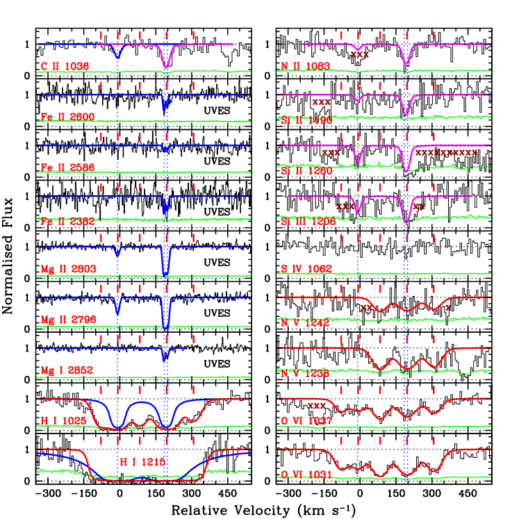
Figure 1.— Velocity plots of different transitions covered in the $\it HST/$COS and $\it VLT/$UVES spectra. The zero velocity corresponds to the redshift of the host-galaxy, i.e. $z_{\rm gal}$ = 0.39853. The best fitting Voigt profiles for high- (low-) ions are shown in smooth red (blue) curves on top of data. In the Ly$\alpha$ and Ly$\beta$ panels the blue and red curves indicate the contributions of low- and high-ionization gas phases, respectively (Appendix A). The magenta curves represent synthetic profiles corresponding to our adopted PI models for the low-ions (Appendix B.2), since the COS spectrum is noisy and does not have enough resolution to resolve the narrow lines. Error in the normalized flux is shown in green histogram. The vertical blue dotted lines represent the line centroids of the Mg ii components. The small red ticks in each panel show the line centroids of the O vi components. Unrelated absorption are marked by ‘x’ symbols. Note that O vi $\lambda$1037 model subtracted spectrum is shown in the C ii $\lambda$1036 panel.

III.1. Absorption Analysis

The Ly$\alpha$, Ly$\beta$ and different ionic transitions originating from the $z_{\rm abs}$ = 0.39853 absorber are shown in Figure 1. Mg ii absorption, covered by the high resolution UVES spectrum, is detected in three velocity components. We refer to them as L–1 ($v\sim-10$  km s^-1), L–2 ($v\sim+180$  km s^-1), and L–3 ($v\sim+200$  km s^-1). Mg i absorption is detected only in the two strong Mg ii components at $v\sim+200$ km s^-1 (i.e. in L–2 and L–3). A weak Fe ii absorption is also detected in these two components. Using the vpfit software we fit Mg i, Mg ii, and Fe ii lines simultaneously assuming the $b$-parameters of magnesium and iron are connected via pure thermal broadening. The Voigt profile fit parameters are summarized in Table 1. In the cases of non-detections, we present standard $3\sigma$ upper limits estimated from the error spectrum.

As we use only the G160M grating data, any transitions with rest-frame wavelength below 1010 Å and above 1270 Å are not covered by the COS spectrum. The detected C ii $\lambda 1036$ and N ii $\lambda 1083$ absorption clearly trace the Mg ii line kinematics seen in the UVES spectrum. However, the component structure at $v\sim+200$ km s^-1 is not resolved due to the lower spectral resolution of COS. Note that the N ii $\lambda 1083$ absorption at $v\sim 0$ km s^-1 is blended with Si iii $\lambda 1206$ absorption from another known intervening system at $z_{\rm abs}$ = 0.25647. The Si ii $\lambda 1193$ is blended with the Galactic Al ii $\lambda 1670$ absorption. The Si ii $\lambda 1190$, $\lambda 1260$ and Si iii $\lambda 1206$ transitions are too noisy to get reasonable fitting parameters. Moreover, the latter two transitions are partially blended by unrelated absorption. As the component structure is not resolved and the data are noisy, except for the weak C ii component at $\sim 0$ km s^-1, we do not attempt to fit the low-ions detected in the COS spectrum. Instead, we generate synthetic profiles corresponding to our adopted PI model (Appendix B.2) and compare with the observed data.

We note here that the line spread function (LSF) of the COS spectrograph is not a Gaussian. A characterization of the non-Gaussian LSF for COS can be found in Ghavamian et al. (2009) and Kriss (2011). For our Voigt profile fit analysis we adopt the latest LSF given by Kriss (2011). The LSF was obtained by interpolating the LSF tables at the observed central wavelength for each absorption line and was convolved with the model Voigt profile while fitting absorption lines or generating synthetic profiles using vpfit. Since there is no Ly$\alpha$ forest crowding at low-$z$ and the interested absorption lines do not fall on top of any emission line, we do not account for the continuum fitting error in the absorption line fit parameters.

The O vi $\lambda\lambda 1031,1037$ absorption is detected over a velocity spread of $>500$ km s^-1. A formal measurement gives $\Delta v_{90}=419$ km s^-1 with an optical depth-weighted absorption redshift of $\bar{z}=0.39909$ (see e.g. Figure 3 of Muzahid et al., 2012). As discussed in Section IV, this is among the four largest velocity spread intervening O vi absorbers at $z<1$ known to date. A minimum of five components are required to fit the O vi doublets satisfactorily. We refer to them as H–1 through H–5 from lowest velocities to highest velocities. Note that the O vi $\lambda 1037$ absorption in the H–1 and H–2 components is blended with the C ii $\lambda 1036$ absorption. The apparent column density profiles do not suggest any hidden saturation in the three redward O vi components (i.e. H–3, H–4, and H–5) which are not affected by the C ii contamination. It is intriguing to note that, unlike most low-$z$ O vi absorbers, strong N v is detected in these three components. However, the N v profiles appear noisy and the N v $\lambda 1242$ line is partially blended. To obtain reasonable fitting parameters we fit both O vi and N v simultaneously assuming pure thermal broadening. A pure non-thermal assumption also provides similar component column densities. Voigt profile fit parameters for these components are given in Table 2. In the cases of non-detections we provide standard $3\sigma$ upper limits.

It is apparent from the Figure 1 that the absorption kinematics of Mg ii and O vi are significantly different. Mg ii shows two distinct absorption clumps at $v\sim-10$ km s^-1 and at $v\sim+200$ km s^-1 with $\Delta v_{90}$ of $\sim 25$ and $\sim 28$ km s^-1, respectively. O vi, on the contrary, shows a contiguous absorption with a $\Delta v_{90}$ of 419 km s^-1. No low-ions are detected in the H–1, H–3, and H–5 components. Mg ii is detected at velocities similar to those of the H–2 and H–4 components. However, the O vi components show much larger $b$-parameters as compared to the Mg ii components. The data, thus, clearly indicate that the absorbing gas has multiple phases with different densities (and/or different temperatures) giving rise to different absorption kinematics.

Here, we refer the reader to Appendix A for a detailed description of how we estimate $N(\mbox{H\,{\sc i}})$ in the different high- and low-ionization absorption components. In brief, we estimate $\log N(\mbox{H\,{\sc i}})$ in the range 18.3–18.6 and 14.6–15.3 for the low- and high-ionization components, respectively.

Table 1Low-ionization metal line fit parameters.

Ion	$z_{\rm abs}$	ID	$b$ (km s-1)	$\log N$ (cm-2)
Mg ii	0.398479$\pm$0.000003	L–1	9.1$\pm$0.8	12.44$\pm$0.03
C ii			9.1	13.90$\pm$0.14
Fe ii			9.1	$<$12.5
Ca ii			9.1	$<$11.3
Mg i			9.1	$<$11.2
Na i			9.1	$<$11.6
H i			9.1a	$<$18.6
Mg ii	0.399384$\pm$0.000002	L–2	4.8$\pm$0.5	13.24$\pm$0.08
Fe ii			3.1$\pm$0.5	12.66$\pm$0.10
Ca ii			4.8	$<$11.2
Mg i			4.8$\pm$0.5	11.62$\pm$0.05
Na i			4.8	$<$11.6
H i			4.8a	$<$18.3
Mg ii	0.399449$\pm$0.000003	L–3	6.7$\pm$0.6	13.11$\pm$0.04
Fe ii			4.4$\pm$0.6	12.56$\pm$0.10
Ca ii			6.7	$<$11.3
Mg i			6.7$\pm$0.6	11.53$\pm$0.06
Na i			6.7	$<$11.4
H i			6.7a	$<$18.3

Notes – All column density upper limits are quoted at $3\sigma$ as estimated from the error spectrum for the adopted $b$-parameter. ^aThe $b$-values are too low for the gas temperature we derived under PI equilibrium conditions (i.e. $T\sim 10^{4}$ K). However, we found that the $N(\mbox{H\,{\sc i}})$ limits remain unchanged for $b$-parameters of 14–20 km s^-1 as suggested by our PI models in Appendix B.

III.2. Galaxy Analysis

The $HST/$WFPC2 F702W image of the Q 0122–003 field is shown in the left panel of Figure 2. There are seven galaxies with confirmed spectroscopic redshifts (see Table LABEL:tab:zfield for details). Galaxy apparent Vega-magnitudes were determined using 1.5$\sigma$ isophotes from Source Extractor (Bertin & Arnouts, 1996). The sky orientation parameters, such as inclination angles ($i$) and azimuthal angles ($\Phi$), for all these galaxies were measured using GIM2D (Simard et al., 2002) following the methods of Kacprzak et al. (2011). Here we define the azimuthal angle such that at $\Phi=0^{\circ}$ the quasar line-of-sight lies along the galaxy projected major axis, and at $\Phi=90^{\circ}$ it lies along the projected minor axis.

We use our own fitting program (FITTER: see Churchill et al., 2000), which computes best fit Gaussian amplitudes, line centers, and widths, in order to obtain emission-line redshifts and line fluxes. The galaxy redshifts as listed in Table LABEL:tab:zfield have accuracy ranges from 6 – 15 km s^-1. Here we focus our study on the $z_{\rm gal}$ $=0.39853$ galaxy and will present detailed analysis on the other galaxies in future works. We show them here to demonstrate the spectroscopic completeness of the field. Note that no other galaxy redshift matches the absorption redshift within $\Delta v\gtrsim\pm 1000$  km s^-1, suggesting that the host-galaxy is isolated. The host-galaxy has an impact parameter $D=163$ kpc, $i=63^{\circ}$ and $\Phi=73^{\circ}$.

The SFR of the host-galaxy is estimated from the H$\alpha$ luminosity using the relation of Hao et al. (2011). The measured H$\alpha$ flux of $2.69\times 10^{-15}$ erg cm^-2 s^-1, corresponding to a luminosity of $1.50\times 10^{42}$  erg s^-1, leads to a SFR of 6.9 $M_{\odot}$ yr^-1. Using the effective radius (3.5 kpc) and ellipticity (0.56) obtained from the GIM2D model we derive a star-formation rate density of $\Sigma_{\ast}=$ 0.4 $M_{\odot}$ yr^-1 kpc^-2. This is a factor of 4 higher than the known $\Sigma_{\ast}$ threshold for driving galactic-scale outflows in local starbursts (Heckman, 2003). The observed O iii$/$H$\beta$ and N ii$/$H$\alpha$ emission line ratios (i.e. $-0.323$ and $-0.391$ dex respectively) suggest that while most of the emission is due to star formation, some AGN contamination could also be present (Baldwin et al., 1981). Thus, strictly speaking, the measured SFR and $\Sigma_{\ast}$ should be considered as upper limit. We compute a gas-phase oxygen abundance for the host-galaxy using the N2 relation of Pettini (2004) where 12+${\rm\log(O/H)}$=8.90+0.57$\times$N2 (N2 $\equiv$ log(N ii/H$\alpha$)).

The galaxy halo mass $M_{\rm\,h}$ was obtained by halo abundance matching. We used the methods described in Churchill et al. (2013a). Systematics and uncertainties in the method are elaborated in Churchill et al. (2013b). The halo mass library is drawn from the Bolshoi $N$-body cosmological simulation (Klypin et al., 2011) and is matched to the observed $r$-band luminosity function from the COMBO-17 survey (Wolf et al., 2003). The galaxy $r$-band and $B$-band absolute magnitudes, $M_{r}$ and $M_{B}$ (respectively), were determined by $K$-correcting (e.g., Kim et al., 1996) the $HST/$WFPC2 F702W observed magnitude using the Coleman et al. (1980) spectral energy distributions (SED) from Bolzonella et al. (2000). The $K$-correction is fully described in Nielsen et al. (2013b). The galaxy $B$-band luminosity, i.e. $L_{B}/L_{B}^{\ast}=0.5$, was calculated by using the linear fit to $M_{B}^{\ast}$ with redshift from Faber et al. (2007). We have no color information for the galaxy. Given the late-type appearance of the galaxy morphology in the WFPC2 image (see the top-right panel of Figure 2), we adopt the Sbc SED for the $K$-correction. The adopted halo mass is $\log M_{\rm\,h}/M_{\odot}=12.48\pm 0.16$. The $K$-correction varies by no more than $0.46$ from an Irr to an E SED, which translates to a halo mass range of $\log M_{\rm\,h}/M_{\odot}=12.4$–$12.7$, respectively, across the range of “normal” galaxy SEDs.

The galaxy virial radius, $R_{\rm vir}$, is obtained using the formalism of Bryan & Norman (1998). We obtained $R_{\rm vir}=278_{-32}^{+38}$ kpc, where the uncertainty accounts for the uncertainty in the adopted $M_{\rm\,h}$. For the line-of-sight impact parameter, we probe the CGM of this galaxy with respect to the virial radius at the projected location of $D/R_{\rm vir}=0.6$.

Table 2High-ionization metal line fit parameters.

Ion	$z_{\rm abs}$	ID	$b$ (km s-1)	$\log N$ (cm-2)
O vi	0.398153$\pm$ 0.000023	H–1	28.3$\pm$ 6.3	14.26$\pm$ 0.09
N v			28.3	$<$13.7
S iv			28.3	$<$14.0
H i			28.3	$<$14.9 (15.04$\pm$0.09)
O vi	0.398481$\pm$ 0.000026	H–2	35.4$\pm$10.5	14.28$\pm$ 0.09
N v			35.4	$<$13.7
S iv			35.4	$<$14.0
H i			35.4	$<$15.2 (15.36$\pm$0.11)
O vi	0.398913$\pm$ 0.000009	H–3	32.5$\pm$ 3.2	14.62$\pm$ 0.03
N v			34.7$\pm$ 0.0a	14.22$\pm$ 0.08
S iv			32.5	$<$14.1
Si iii			32.5	$<$12.8
H i			32.5	$<$14.8 (14.83$\pm$0.05)
O vi	0.399443$\pm$ 0.000009	H–4	42.4$\pm$ 3.6	14.61$\pm$ 0.02
N v			45.3$\pm$ 0.0a	14.28$\pm$ 0.06
S iv			42.4	$<$14.2
H i			42.4	$<$15.3 (15.35$\pm$0.05)
O vi	0.399964$\pm$ 0.000010	H–5	32.5$\pm$ 3.2	14.38$\pm$ 0.03
N v			34.8$\pm$ 0.0a	14.12$\pm$ 0.08
S iv			32.5	$<$14.1
Si iii			32.5	$<$12.8
H i			32.5	$<$14.6 (14.64$\pm$0.04)
C ivb	(AOD measurements)		191	$>$14.7

Notes – All column density upper limits are quoted at $3\sigma$ as estimated from the error spectrum for the adopted $b$-parameter. The $N(\mbox{H\,{\sc i}})$ values in the parenthesis are obtained assuming that the Ly$\beta$ profile is entirely due to the high-ionization absorption components (see Appendix A) with $b$-parameters tied with $b(\mbox{O\,{\sc vi}})$. ^a$b(\mbox{N\,{\sc v}})$ are tied with $b(\mbox{O\,{\sc vi}})$ via thermal broadening. ^bApparent Optical Depth (AOD) measurements using FOS spectrum.

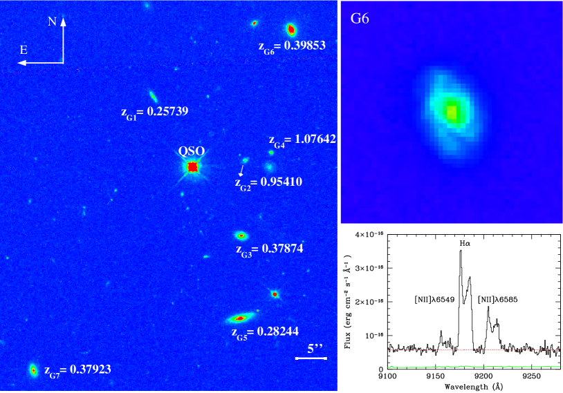
Figure 2.— The $HST/$WFPC2 F702W image of the Q 0122–003 field on the left, with spectroscopic redshifts of the various galaxies labelled. The top right is a $5\times 5^{\prime\prime}$ zoomed in view of the galaxy of interest, at $z_{\rm gal}=0.39853$, which is classified as an Sbc galaxy. A part of the galaxy spectrum, obtained with the $\it KECK/$ESI, covering H$\alpha$ and N ii emission lines, is shown in the lower right panel. The data are shown in black, a continuum fit is shown in red and the error or sigma spectrum is shown in green.

Table 3Redshifts and properties of the galaxies in the Q 0122–003 field.

Galaxy ID	RA	Dec	$m_{\rm F702W}$	$D$ (′′)	$D$ (kpc)	$z_{\rm{gal}}$	$i$ (degrees)	$\Phi$ (degrees)
Q 0122–003G1	01:25:29.29	$-$00:05:43.13	21.5	14.44	57.7$\pm$0.3	0.25739$\pm$0.000050	$85.0_{-1.4}^{+0.0}$	$3.0_{-1.4}^{+1.2}$
Q 0122–003G2	01:25:28.21	$-$00:05:54.64	22.2	9.66	76.5$\pm$1.3	0.95410$\pm$0.000095	$60.5_{-26.7}^{+18.2}$	$13.8_{-19.8}^{+45.2}$
Q 0122–003G3	01:25:28.26	$-$00:06:08.20	20.4	15.18	78.9$\pm$0.3	0.37874$\pm$0.000022	$68.9_{-1.8}^{+2.0}$	$57.5_{-3.3}^{+2.4}$
Q 0122–003G4	01:25:27.91	$-$00:05:53:17	22.3	14.39	117.2$\pm$0.4	1.07642$\pm$0.000069	$85.0_{-6.3}^{+0.0}$	$7.4_{-11.4}^{+12.9}$
Q 0122–003G5	01:25:28.27	$-$00:06:23.03	19.5	28.59	122.2$\pm$0.8	0.28244$\pm$0.000021	$84.3_{-0.6}^{+0.7}$	$84.9_{-0.4}^{+1.0}$
Q 0122–003G6	01:25:27.67	$-$00:05:31.39	19.4	30.39	163.0$\pm$0.1	0.39853$\pm$0.000027	$63.2_{-2.6}^{+1.7}$	$73.4_{-4.6}^{+4.7}$
Q 0122–003G7	01:25:30.68	$-$00:06:32.43	20.3	45.98	239.2$\pm$0.1	0.37923$\pm$0.000029	$56.1_{-8.2}^{+10.4}$	$44.7_{-1.9}^{+2.6}$

III.3. Photoionization modeling

In order to understand the physical conditions and the chemical abundances in the absorbing gas we run grids of PI models using cloudy (v13.03, last described by Ferland et al., 2013). In these models absorbing gas is assumed to be a plane parallel slab, exposed to the extra-galactic UV background radiation at $z=0.39$ (as computed by Haardt & Madau, 2012) from one side. Here we do not consider the effect of a galaxy/stellar radiation field, as it is negligible at this redshift at a large separation ($\gtrsim$ 100 kpc) from bright ($\sim L_{\ast}$) galaxies (e.g. Narayanan et al., 2010; Werk et al., 2014). We note that the host-galaxy for the present system has $L=0.5L_{B}^{\ast}$ with an impact parameter of 163 kpc. In our models, the relative abundances of heavy elements are assumed to be solar as in Asplund et al. (2009).

Note that here we estimate the average ionization conditions and abundances for the high- and low-ionization gas using the total column densities of relevant ions and H i. Total column density is derived by summing the component column densities presented in Table 1 and 2. We refer the interested readers to Appendix B for a detailed component-by-component ionization modeling for both the high- and low-ionization phases. In Appendix B we have explored both PI and collisional ionization equilibrium (CIE) and non-equilibrium (non-CIE) models for the high-ionization phase. Moreover, we ruled out both the CIE and non-CIE scenarios for the O vi bearing high-ionization gas using several observational constraints such as: (i) the Ly$\beta$ profile is too narrow to explain the required gas temperature, (ii) the presence of strong C iv in the FOS spectrum and (iii) the non-detection of S iv and Si iii absorption. The average chemical/ionization conditions that we present in this section are in good agreement with those from component-by-component analyses. The average model parameters thus provide an adequate description of the high- and low-ionization gas phases.

As illustrated in the left panel of Figure 3, the density of the high-ionization phase, derived using the $N(\mbox{N\,{\sc v}})$ to $N(\mbox{O\,{\sc vi}})$ ratio, is $-4.15\leqslant\log n_{\rm H}\leqslant-4.00$ corresponding to an ionization parameter of $-1.70\geqslant\log U\geqslant-1.85$. For this given density, a super-solar metallicity, i.e. $\rm[X/H]\gtrsim 0.3$, is required to reproduce the observed column densities of O vi and N v. This PI solution produced considerable amounts of C iii ($\log N=14.9$) and C iv ($\log N=15.3$) but did not produce any other detectable low-ions (e.g. C ii, Si iii).

PI models for the low-ionization gas are presented in the right panel of Figure 3. The density is constrained to be $-2.75\leqslant\log n_{\rm H}\leqslant-2.40$ (i.e. $-3.10~{}\geqslant~{}\log~{}U~{}\geqslant~{}-~{}3.45$) from the $N(\mbox{Mg\,{\sc i}})$ to $N(\mbox{Mg\,{\sc ii}})$ ratio. A metallicity of $\rm[X/H]\gtrsim-1.4$ is needed to explain the observed column densities of Mg i and Mg ii simultaneously. Such a solution does not produce a significant amount of N v and/or O vi.

In Table LABEL:tab_models we summarize the PI model parameters. The large total hydrogen column densities (i.e. $\log N_{\rm H}>19.0$) suggest that a significant amount of baryons is associated with both phases. The thicknesses ($L_{\rm los}$) of the two phases are tens of kpc and differ from each other by only a factor of $\sim 3$. But, the density of the low-ionization phase is $\sim 30$ times higher than that of the high-ionization phase. Most interestingly, the metallicity of the high-ionization phase is over an order of magnitude higher than the low-ionization gas phase. The data clearly indicate different origins of the high- and low-ionization gas phases.

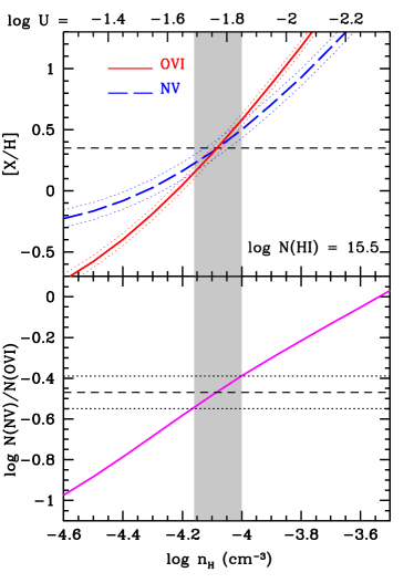
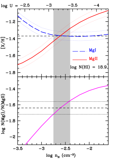
Figure 3.— Average PI models for the high- (left) and low- (right) ionization gas. Bottom panels: The estimation of density/ionization parameters using ionic ratios. The horizontal dashed and dotted lines represent the observed column density ratios and their $1\sigma$ uncertainties, respectively. The shaded regions indicate the density ranges over which model column density ratios (magenta curves) match with the observed values. The ionization parameters corresponding to different $n_{\rm H}$ values are labelled at the top of each panel. Top panels: Metallicity required to reproduce the observed column densities of high- (O vi and N v) and low- (Mg i and Mg ii) ions are plotted in thick curves as a function of gas density. The dotted curves correspond to $1\sigma$ uncertainties in respective column density measurements. The $N(\mbox{H\,{\sc i}})$ values assumed by the models are mentioned. The horizontal dotted lines represent the average metallicities. Over an order of magnitude difference in metallicity between the high- and low-ionization gas phases is apparent.

Table 4Summary of PI model parameters.

Phase	$\log n_{\rm H}$	$\log U$	$>\rm[X/H]$	$>\log N_{\rm H}$	$>L_{\rm los}$
	(cm-3)			(cm-2)	(kpc)
High	$-4.1$	$-1.75$	0.3	19.1	53
Low	$-2.6$	$-3.25$	$-1.4$	20.2	19

IV. Discussion

IV.1. The strong and large velocity spread O vi absorption

We have presented a detailed analysis of an ultra-strong intervening O vi absorber at $z_{\rm abs}$ = 0.39853 detected in the $HST/$COS spectrum of Q 0122–003. The absorber exhibits $\log N(\mbox{O\,{\sc vi}})=15.16\pm 0.04$ with a kinematic spread of $\Delta v_{90}=419$  km s^-1. Such a strong (i.e. $\log N>15.0$) and large velocity spread (i.e. $>400$  km s^-1) intervening O vi systems are very rare in the Milky Way halo (Wakker et al., 2003; Savage et al., 2003), in high-velocity clouds (HVCs; Sembach et al., 2003), in the CGM (Werk et al., 2014) and in the IGM (Tripp et al., 2008; Muzahid et al., 2012; Savage et al., 2014). For example, only $2/42$ systems in the COS-Halos sample show $\log N(\mbox{O\,{\sc vi}})>15.0$ (Tumlinson et al., 2011b). In a blind survey of intergalactic O vi absorbers at high-$z$ ($1.9<z<3.1$) Muzahid et al. (2012) have found only $3/85$ systems with $\Delta v_{90}>200$  km s^-1 with none of them having $\Delta v_{90}>400$  km s^-1. The systems with large $\Delta v_{90}$, in their sample, are thought to be associated with outflows from Lyman Break Galaxies (LBGs; see also Adelberger et al., 2003, 2005). The only known O vi absorbers at low-$z$ with $\Delta v_{90}$ in excess of 400 km s^-1 are the $z_{\rm abs}$ = 0.3558 system towards J 1009+0713 (Tumlinson et al., 2011a), the $z_{\rm abs}$ = 0.927 system towards PG 1206+459 (Fox et al., 2013) and the $z_{\rm abs}$ = 0.227 systems towards the QSO pair Q 0107–025A and Q 0107–025B (Muzahid, 2014). Tripp et al. (2011) have argued that a post-starburst outflow is responsible for the wide velocity spread absorption seen towards PG 1206+459 (but see Ding et al., 2003, for an alternate explanation). Tumlinson et al. (2011a) have suggested that O vi arises from interfaces between “cool” and “hot” gas phases. Moreover, Muzahid (2014) has conjectured that the large velocity spread O vi absorption seen through the pair of lines-of-sight is originating from an “ancient outflow” (see e.g. Ford et al., 2014).

Recently, in 15 of 20 Lyman limit systems (LLS) with $\log N(\mbox{H\,{\sc i}})>17.3$ at $2<z<3.5$, Lehner et al. (2014) have reported presence of strong (e.g. average $\log N(\mbox{O\,{\sc vi}})=14.9\pm 0.3$) and wide velocity spread i.e. $200<\Delta v<400$ km s^-1 O vi absorption in the ISM/CGM of high-$z$ galaxies and hypothesized that these strong CGM O vi absorbers probe outflows of star-forming galaxies (see also Fox et al., 2007). We note that, a vast majority of local starburst galaxies show ultra-strong “down-the-barrel” O vi absorption with an average column density of $\log N(\mbox{O\,{\sc vi}})=15.0\pm 0.3$ (Grimes et al., 2009). Additionally, these O vi absorption lines are broad with a FHWM of $\sim 367\pm 95$ km s^-1.

In summary, intervening O vi absorbers with $\log N>15.0$ and $\Delta v_{90}>400$ km s^-1, as observed in the present system, are extremely rare. Large-scale galaxy outflows are thought to be the most likely origin of such O vi absorbers whenever detected. The frequent occurrence of strong and large velocity spread O vi absorption in local starburst galaxies further strengthens this idea.

IV.2. The presence of strong N v absorption

Unlike most low-$z$ intervening O vi absorbers, the present system shows an ultra-strong ($\log N(\mbox{N\,{\sc v}})=$  $14.69\pm 0.07$) and wide-spread ($\Delta v_{90}=285$ km s^-1) N v absorption with $\log N(\mbox{N\,{\sc v}})/N(\mbox{O\,{\sc vi}})$  $=-0.47\pm 0.08$. As the creation and destruction ionization potentials of N v are 77.5 eV and 97.9 eV respectively, a hard radiation field at energies above 4 Ryd is required to ionize nitrogen to its $\rm N^{+4}$ ionization state. Though no systematic survey exists, weak N v absorption ($<10^{14}$ cm^-2) is detected in only a handful of O vi systems at low-$z$ (e.g. $z_{\rm abs}$ = 0.20260 system towards PKS 0312–77 (Lehner et al., 2009), $z_{\rm abs}$ = 0.16716 system towards PKS 0405–123 (Savage et al., 2010), $z_{\rm abs}$ = 0.227 towards Q 0107–025A (Muzahid, 2014)). In all of them O vi is found to be fairly strong ($>10^{14.7}$ cm^-2). Here, we note that Werk et al. (2013) have not found any N v absorption with $\log N>14$ in the COS-Halos sample.

To our knowledge, there are only 6 other intervening systems that show $\log N(\mbox{N\,{\sc v}})>14.0$ and only one of them is at $z<1$. These are the $z_{\rm abs}$ = 0.927 system towards PG 1206+459 (Tripp et al., 2011), $z_{\rm abs}$ = 2.811 system towards Q 0528–250 (Fox et al., 2007), $z_{\rm abs}$ = 2.83437 system towards J 1343+5721 and $z_{\rm abs}$ = 2.47958 system towards Q 1603+3820 and $z_{\rm abs}$ = 2.18076 system towards Q 1217+499 (Lehner et al., 2014), and the $z_{\rm abs}$ = 1.5965 system towards PKS 0237–23 (Fechner & Richter, 2009). Interestingly, all these systems show strong O vi ($\log N>14.8$) absorption kinematically spread over $>200$  km s^-1 similar to the present system, and all of them are LLS.

A population of photoionized intervening N v absorbers, with $d{\mathcal{N}}/dz\sim 0.9$ down to $\log N=12.7$, at high-$z$ ($1.5<z<2.5$) is reported by Fechner & Richter (2009). These absorbers are predominantly weak and only one out of 21 systems shows $\log N(\mbox{N\,{\sc v}})>14.0$. As the intensity of the extra-galactic UV background radiation is considerably higher as compared to low-$z$ due to the enhanced QSO activity at $z\sim 2$ (Haardt & Madau, 1996; Khaire & Srianand, 2015), detection of weak N v absorption at high-$z$ is consistent with expectations for PI models. However, the presence of N v with $\log N>14.0$ is very rare at any redshift.

Apart from the present system, the only other O vi absorber with $\log N(\mbox{N\,{\sc v}})>14.0$ at $z<1.0$ is the well known system at $z_{\rm abs}$ = 0.927 towards PG 1206+459 (Churchill & Charlton, 1999; Ding et al., 2003; Tripp et al., 2011). These two systems have remarkable resemblance in the absorption properties of their high-ions and show $\log N(\mbox{N\,{\sc v}})/N(\mbox{O\,{\sc vi}})\sim-0.5$ (Rosenwasser et al., in preparation). Unlike Tripp et al. (2011), who favored a collisional ionization scenario for N v and could not estimate a high-ionization phase metallicity, Rosenwasser et al. have found that both O vi and N v can be explained under PI equilibrium with solar to super-solar metallicities and with a density of $\sim 10^{-4}$ cm^-3. As we discuss next, all these properties are strikingly similar to what we deduce for the present system.

Very strong N v absorption is characteristic of many intrinsic narrow and mini-broad absorption line systems, that are known to be related to the AGN winds/host-galaxy because of a velocity within $\sim$ 5000 km s^-1 of the QSO redshift, and evidence of partial coverage of the QSO continuum/broad emission line source (Hamann et al., 2000; Srianand et al., 2002; Misawa et al., 2007; Wu et al., 2010). For example, Wu et al. (2010) reported three $2.6<z<3.0$ intrinsic N v absorbers with metallicities greater than 10 times the solar value. Strong O vi and C iv absorption are common in these systems as well. The present system is clearly not an intrinsic absorber, but the common properties are likely evidence of an origin in the high metallicity, central region of a galaxy. Both the material that feeds an AGN wind, and that which is ejected in a starburst outflow share a similar chemical origin in a high metallicity environment (Hamann & Ferland, 1999).

IV.3. Origins of different gas phases

In Section III.3 we have demonstrated that the O vi bearing gas in this absorber can be explained with PI equilibrium models that require a density of $\sim 10^{-4.1}$ cm^-3, a super-solar metallicity (i.e. $\rm[X/H]\gtrsim 0.3$), and a solar $\rm[N/O]$ ratio. The synthesis of N can arise from primary and secondary production via the CNO cycle. Primary production is synthesis of N from C produced in the core of the same star via helium burning and secondary production is the synthesis of N from C and O produced in previous generations of stars. Secondary N enrichment of the ISM occurs well after massive stars have gone Type-II supernovae and seeded the ISM with oxygen. For enrichment from primary synthesis, the $\rm[N/O]$ ratio is roughly $-0.6$ for $\rm[O/H]\lesssim-0.3$. For enrichment from secondary synthesis, the $\rm[N/O]$ ratio increases with increasing metallicity for $\rm[O/H]\gtrsim-0.3$, such that by $\rm[O/H]\simeq+0.3$, $\rm[N/O]\simeq 0.0$ i.e. the solar value (e.g. see Figure 9 of Pettini et al., 2008). Therefore, the assumption of a solar $\rm[N/O]$ ratio in this system is reasonable. Solar/super-solar metallicity with solar $\rm[N/O]$ ratio suggests that nitrogen in the high-ionization absorbing gas is predominantly produced via the secondary channel. Thus, the high-ionization, low density gas phase is likely to be originating from a region of the galaxy with a prolonged and high star formation rate (see also Hussain et al., 2015). This is consistent with the host-galaxy properties as discussed in the next section.

It is often claimed that strong O vi absorbers are collisionally ionized (e.g. Lehner et al., 2014) as they require unreasonably large sizes under PI equilibrium (but see Muzahid, 2014). However, from the observed narrowness of the Ly$\beta$ profile, the non-detection of S iv absorption, and the presence of strong C iv absorption in the low-resolution FOS spectrum, we have ruled out the possibility of O vi bearing gas in this system being collisionally ionized (Appendix B.3 and B.4).

For the low-ionization phase, both the overall (Section III.3) and the component-by-component (Appendix B.2) approach of PI modeling suggest a metallicity of $\rm[X/H]\gtrsim-2.0$ to $-1.3$. The high-ionization phase has more than a factor of $\sim 10$ higher metallicity. This is in contrast to the $z_{\rm abs}$ = 0.927 system towards PG 1206+459 for which Rosenwasser et al. (in preparation) have found that the solar/super-solar metallicity of the low-ionization gas is indeed similar to the high-ionization gas. We note that in the present case there is no one-to-one correspondence between the high- (e.g. O vi) and low- (e.g. Mg ii) ionization absorption kinematics. But in the case of PG 1206+459 kinematic similarity between Mg ii and O vi absorption is quite remarkable. Therefore, while for PG 1206+459 both the high- and low-ionization gas phases are consistent with being part of same multiphase outflow (e.g. Tripp et al., 2011), the low-ionization phase in the present system likely has a very different origin from the high-ionization phase.

Using the methods of Kacprzak et al. (2010), we measured the rotation curve of the host-galaxy from the H$\alpha$ emission line, which extends $\pm 1^{\prime\prime}$ (corresponding to 3.5 kpc) from the galaxy center. The projected rotation velocity is $\simeq 200$ km s^-1. We then employed the rotation model of Steidel et al. (2002) to examine the range of allowed velocities along the line-of-sight that are consistent with extended galaxy rotation given the galaxy inclination, azimuthal angle, the quasar impact parameter, and the gas scale height, $h_{\nu}$. Following Kacprzak et al. (2010), we use $h_{\nu}=1$ Mpc (for a non lagging halo above the galaxy plane). The range of velocities along the line-of-sight that could be due to extended rotation from the galaxy are $+25\leq v\leq+150$ km s^-1. The components of the low-ionization gas are at $v~{}\simeq 0$ and $v\simeq 200$  km s^-1, as probed with Mg ii absorption. None of the Mg ii components is consistent with co-rotation of the galaxy. The low metallicity and kinematics of this phase perhaps suggest that it stems from recycled gas as seen in numerical simulation of Oppenheimer et al. (2010). Such an interpretation is also supported by the recent study of “bimodal” metallicity distribution of low-ions in low-$z$ LLS by Lehner et al. (2013). The metal-poor branch, possibly tracing cold accretion streams, in their sample peaks at $\rm[X/H]=-1.6$ which is consistent with what we find for this system.

IV.4. The host-galaxy

At the epoch of our measurement, the host galaxy has a high SFR of $6.9~{}M_{\odot}$ yr^-1 and a $\Sigma_{\ast}$ of $\sim 0.4~{}M_{\odot}$ yr^-1 kpc^-2, the latter being a factor of $\sim 4$ above the well known threshold of 0.1 $M_{\odot}$ yr^-1 kpc^-2 for driving galactic-scale winds (Heckman, 2003). The observed galaxy orientation parameters, i.e. $i=63^{\circ}$ and $\Phi=73^{\circ}$, as given in Table LABEL:tab:zfield suggest that the QSO line-of-sight is at ideal position to pierce one of the bicones of a bi-conical outflow propagating along the minor-axis of the galaxy (e.g. Bouché et al., 2012; Kacprzak et al., 2012, 2014; Bordoloi et al., 2014b; Schroetter et al., 2015). The host-galaxy has a metallicity of $\rm 12+\log(O/H)=$  $8.68\pm 0.02$, i.e. $\rm[O/H]\sim 0.0$, which is roughly consistent with the metallicity of high-ionization gas phase. All these observational evidences strongly indicate that the high-ionization gas, as probed by the ultra-strong O vi and N v absorption, is tracing a powerful (see the next section), active, metal-enriched, large-scale galactic outflow.

Here we emphasize that the absorber is unlikely from the ISM of a dwarf galaxy that happens to be coincident on the quasar. van Zee & Haynes (2006) found that the H ii regions of dwarf galaxies have sub-solar metallicity and $\rm[N/O]$ ratios consistent with primary N synthesis. On the other hand, van Zee et al. (1998) showed that the H ii regions of massive spiral galaxies have solar to super-solar metallicity and $\rm[N/O]$ ratios consistent with secondary N synthesis. As such, we favor the scenario in which the high-ionization absorbing gas was ejected from the host spiral galaxy we have identified at the absorption redshift.

IV.5. The outflow properties

From the halo mass ($M_{h}\sim 10^{12.5}M_{\odot}$) and the virial radius ($R_{\rm vir}\sim 280$  kpc) of the host-galaxy we estimate a circular velocity of $v_{c}\sim 220$  km s^-1. Using the relationship between SFR, $v_{c}$, and the terminal outflow speed ($v_{w}$) by Sharma & Nath (2012) we estimate $v_{w}\sim 230$ km s^-1. Here we note that $v_{c}$ is calculated at $R_{\rm 200}$ in their models whereas we compute $v_{c}$ at the virial radius. Nevertheless, this does not change our estimated $v_{w}$ by more that a few percent. An outflow with a constant speed of 230  km s^-1 would require 0.7 Gyr time to travel the minimum projected distance of 163 kpc. This is on the order of the sound crossing time for the individual cool ($T\sim 10^{4}$ K) photoionized clouds with size $\sim 4-10$  kpc (see Appendix B.2). However, in practice the outflow could have been ejected with a significantly higher speed as compared to the terminal speed we estimate here. In that case the flow time could be significantly lower as compared to the sound crossing time so that the clouds would have enough time to be stable against any mechanical disturbances before they traverse a distance of 163 kpc.

Under the thin-shell approximation the mass of the outflowing gas can be written as: $M_{\rm out}=4\pi\mu m_{p}C_{\Omega}C_{f}N_{\rm H}r^{2}$, where $m_{p}$ is the proton mass, $\mu=1.4$ accounts for the mass of helium, $C_{\Omega}$ $(C_{f})$ is the global (local) covering factor, and $r$ is the thin-shell radius (e.g. Rupke et al., 2005). The global covering factor is related to the wind’s opening angle. Here we assume $C_{\Omega}=0.4$ as observed in local starbursts (e.g. Veilleux et al., 2005). The local covering factor, on the other hand, is related to the wind’s clumpiness. For simplicity we assume it to be unity for the high-ionization, low density, diffuse gas. Using $r=$ 163 kpc and $N_{\rm H}=10^{19.1}$  cm^-2 (see Table LABEL:tab_models) we estimate $M_{\rm out}\sim 2\times 10^{10}M_{\odot}$ corresponding to an oxygen mass of $M_{\rm O}\sim 10^{7}~{}M_{\odot}$. These are consistent with the masses as estimated in the CGM of $\sim L_{\ast}$ galaxies at $z\lesssim 0.2$ by Tumlinson et al. (2011b). Using the wind speed of 230 km s^-1, we further estimate the mass-flow rate of $\dot{M}_{\rm out}\sim 54~{}M_{\odot}$  yr^-1 and the kinetic luminosity of $\dot{E_{k}}\sim 9\times 10^{41}$ erg s^-1 (see Appendix C). These values are typical of what have been seen in “down-the-barrel” outflows from infrared-luminous starbursts at $z<0.5$ (i.e. Rupke et al., 2005).

To better understand how the mass outflow rate is related to the SFR of the host galaxy, it is customary to define the mass loading factor, $\eta\equiv\dot{M}_{\rm out}/\rm SFR$, which is a critical ingredient for numerical simulations of structure formation (e.g. Oppenheimer et al., 2010; Davé et al., 2011b). We estimate a $\eta$ of $\sim 8$ for the outflow studied here. In the infrared-luminous starbursts sample of Rupke et al. (2005), $\eta$ is found to range from 0.001 to 10 but is $\sim 0.1$ on an average. However, we note that a vast majority of these starburst galaxies have SFR $>100~{}M_{\odot}~{}\rm yr^{-1}$ which is significantly higher as compared to the present galaxy with SFR of $6.9~{}M_{\odot}~{}\rm yr^{-1}$. Therefore, the galaxy in our study is extremely efficient in entraining mass, in the form of outflow, for its SFR. This probably because of the high $\Sigma_{\ast}$. However, it might also be possible that the host-galaxy had much higher SFR at the epoch of ejection compared to what we observe today.

V. Summary

We have examined the physical conditions, chemical abundances, and energetics of a large-scale galactic outflow in the CGM of a star-forming (SFR $6.9~{}M_{\odot}$ yr^-1), sub-$L_{\ast}$ ($0.5L_{B}^{\ast}$) galaxy at $z=0.39853$. Using the halo abundance matching technique we estimate a halo mass of $M_{h}\sim 10^{12.5\pm 0.2}M_{\odot}$ and a virial radius of $R_{\rm vir}\sim 280$ kpc for the galaxy. Along with Ly$\alpha$ and Ly$\beta$, several low- (i.e. Mg i, Mg ii, C ii, N ii, Si ii, Si iii) and high- (i.e. C iv, N v, O vi) ionization metal absorption lines, originating from the CGM of the galaxy, have been detected in the $HST$(COS, FOS) and $VLT$(UVES) spectra of the background quasar Q 0122–003. The QSO is located at an impact parameter of $D=163$ kpc ($D/R_{\rm vir}=0.6$) with an azimuthal angle of 73^∘ with respect to the galaxy major-axis. Our main findings are as follows:

1. The low-ionization absorption components trace photoionized gas with a density of $n_{\rm H}\sim 10^{-2.6}$ cm^-3 ($\log U\sim-3.2$) and a metallicity of $\rm[X/H]\gtrsim-1.4$. Such a low metallicity gas is consistent with being recycled material in the galaxy halo as predicted in numerical simulations.

2. The high-ionization gas phase shows ultra-strong O vi with $\log N(\mbox{O\,{\sc vi}})=15.16\pm 0.04$ kinematically spread over $\Delta v_{90}=419$  km s^-1. Such a strong and large velocity spread O vi absorber is very rare at any redshift. Among the known astrophysical environments in the local universe, only starburst galaxies show such strong O vi absorption (Grimes et al., 2009).

3. Unlike most intervening O vi systems, this absorber shows ultra-strong and wide velocity spread N v absorption with $\log N(\mbox{N\,{\sc v}})=14.69\pm 0.07$ and $\Delta v_{90}=285$  km s^-1. There is only one system at $z<1$ (i.e. $z_{\rm abs}$ = 0.927 towards PG 1206+459, Tripp et al., 2011) that shows N v as strong as this.

4. It is often claimed that strong O vi absorbers are collisionally ionized as they commonly require large sizes ($>$ Mpc) under PI equilibrium (Lehner et al., 2014). However, for this system our PI models suggest line-of-sight thicknesses for individual components of $\sim 10$ kpc. In fact, based on the $b$-parameter constraints from the Ly$\beta$ profile, the non-detection of S iv, and the presence of strong C iv ($W_{r}=1.7$ Å) in the FOS spectrum, we have ruled out CIE and non-CIE models.

5. The high-ions, O vi and N v, can be well explained as arising in a low-density ($n_{\rm H}\sim 10^{-4.2}$ cm^-3, $\log U\sim-1.6$) photoionized gas with super-solar metallicity ($\rm[X/H]\gtrsim 0.3$) and with solar $\rm[N/O]$ ratio. The super-solar metallicity with a solar $\rm[N/O]$ ratio implies that nitrogen in this system is predominantly produced via secondary synthesis. Thus the high-ionization, low-density gas is presumably stemming from regions of the host-galaxy that have sustained a high star-formation rate for a prolonged period.

6. The measured $\Sigma_{\ast}$ of $\sim 0.4$ $M_{\odot}~{}\rm yr^{-1}~{}\rm kpc^{-2}$ for the host galaxy is a factor of $\sim 4$ higher than the threshold of $\sim 0.1~{}M_{\odot}~{}\rm yr^{-1}~{}kpc^{-2}$ for driving galactic-scale wind as seen in local starbursts. The azimuthal angle of $73^{\circ}$ suggests that the QSO line-of-sight is in ideal position to pierce the bi-conical outflow propagating along the minor-axis of the host-galaxy.

7. Assuming the high-ionization gas is in outflow, we estimate a outflow mass of $M_{\rm out}\sim 2\times 10^{10}~{}M_{\odot}$, mass outflow rate of $\dot{M}_{\rm out}\sim 54~{}M_{\odot}\rm yr^{-1}$, and kinetic luminosity of $\dot{E}_{k}\sim 9\times 10^{41}$ erg s^-1 using a thin-shell model. These values are consistent with that of “down-the-barrel” outflows from infrared-luminous starbursts at $z<0.5$ (Rupke et al., 2005).

8. We estimate a mass loading factor of $\eta\sim 8$. This is among the highest values as seen in infrared-luminous starbursts at low-$z$. However, we note that the SFR of the host-galaxy is significantly lower (by a factor of ten or more) than the starburst galaxies (Rupke et al., 2005). This indicates that the host-galaxy is highly efficient in entraining mass onto the CGM in the form of outflow.

Finally, we emphasize that such powerful, large-scale, metal-rich outflows are the essential component by means of which a galaxy imparts sufficient mechanical and chemical feedbacks that regulates star formation and hence evolution of a galaxy. Finding and analyzing more such unique absorption systems is crucial for a comprehensive understanding of galaxy feedback mechanisms and reinforce galaxy evolution theory with useful observational constraints.

Support for this research was provided by NASA through grants HST GO-13398 from the Space Telescope Science Institute, which is operated by the Association of Universities for Research in Astronomy, Inc., under NASA contract NAS5-26555. GGK acknowledges the support of the Australian Research Council through the award of a Future Fellowship (FT140100933). Some of the data presented here were obtained at the W. M. Keck Observatory, which is operated as a scientific partnership among the California Institute of Technology, the University of California and the National Aeronautics and Space Administration. The Observatory was made possible by the generous financial support of the W. M. Keck Foundation. Observations were supported by Swinburne Keck programs 2014A_W178E, 2014B_W018E, and 2015A_W018E.

Facilities: $\it HST$(COS, WFPC2), $\it KECK$(ESI), $\it VLT$(UVES)

Appendix A Estimation of $N(\mbox{H\,{\sc i}})$ in different low- and high-ionization components

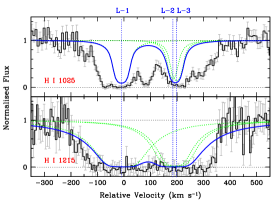
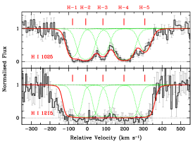
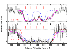
Figure 4.— Estimation of upper limits on $N(\mbox{H\,{\sc i}})$ in different low- (left panel) and high- (middle panel) ionization absorption components. Individual profiles are shown in (green) dotted curves. The resultant profiles are shown in solid curves. The error in each pixel is shown as a grey error-bar. The vertical dotted lines in the left panel are line centroids of the Mg ii components. The small ticks in the middle panel are line centroids of the O vi components. Both low- and high-ionization components are shown in the right panel. Contributions from low- and high-ionization components are shown in (blue) dotted and (red) dashed curves respectively. The resultant solid (magenta) curve explains both the Ly$\alpha$ and Ly$\beta$ profiles satisfactorily.

In this section we describe how $N(\mbox{H\,{\sc i}})$ values in different low- and high-ionization absorption components are estimated. Determining $N(\mbox{H\,{\sc i}})$ component-by-component in a multiphase, multicomponent absorption system is extremely challenging. The presence of unsaturated higher-order Lyman series lines is very helpful in order to disentangle the contributions from high- and low-ionization phases (see e.g. Muzahid, 2014). Our present COS spectrum only covers Ly$\alpha$ and Ly$\beta$ absorption for this absorber. We, therefore, try to estimate conservative upper limits on $N(\mbox{H\,{\sc i}})$ in different low- (L–1 to L–3) and high- (H–1 to H–5) ionization components.

To estimate the maximum allowed $N(\mbox{H\,{\sc i}})$ associated with the low-ionization components, we use the Mg ii component structure and assume pure non-thermal line broadening, i.e. $b(\mbox{H\,{\sc i}})=b(\mbox{Mg\,{\sc ii}})$. This gives the lowest possible $b$-parameters for H i in each component. We then use vpfit to generate synthetic profiles corresponding to different $N(\mbox{H\,{\sc i}})$ values. We start with an initial value of $\log N(\mbox{H\,{\sc i}})=14.0$ and gradually increase the $N(\mbox{H\,{\sc i}})$ value until the synthetic profile just exceeds the observed Ly$\alpha$ and/or Ly$\beta$ profiles. The use of the lowest possible $b(\mbox{H\,{\sc i}})$ values ensures that the $N(\mbox{H\,{\sc i}})$ values we report in Table 1 are indeed conservative. The left panel of Figure 4 shows the synthetic profiles corresponding to the maximum allowed $N(\mbox{H\,{\sc i}})$ values we estimate for the low-ionization components. It is apparent from the bottom panel that the wings of the Ly$\alpha$ absorption are reproduced adequately. Note that because of the assumed low $b$-parameters, $N(\mbox{H\,{\sc i}})$ value as high as $\sim 10^{18.6}$ cm^-2 does not produce any significant Ly$\beta$ optical depth. Therefore, almost all the Ly$\beta$ absorption and the remaining absorption seen in Ly$\alpha$ must arise from the high-ionization components. As mentioned in the footnote of Table 1 our $N(\mbox{H\,{\sc i}})$ limits remain unaltered for $b$-values in the range 14 – 20 km s^-1 which is expected from the PI model temperatures.

To estimate the maximum allowed $N(\mbox{H\,{\sc i}})$ corresponding to the high-ionization components, we use the O vi component structure and again assume pure non-thermal line broadening, i.e. $b(\mbox{H\,{\sc i}})=b(\mbox{O\,{\sc vi}})$. Similar to the low-ionization components, the assumption of pure non-thermal broadening ensures that the $N(\mbox{H\,{\sc i}})$ upper limits for the high-ionization components are conservative as well. We fit the remaining absorption (i.e. after accounting for the contribution from the low-ionization components) using vpfit by allowing the code to vary $N(\mbox{H\,{\sc i}})$. The maximum allowed $N(\mbox{H\,{\sc i}})$ for the high-ionization components are given in Table 2. In the middle panel of Figure 4 we show the corresponding profiles as dotted curves. The solid curve represents the resultant profile. We emphasize here that due to the presence of low-ionization components at similar velocities, the $N(\mbox{H\,{\sc i}})$ limits for the components H–2 and H–4 are uncertain. However, the $N(\mbox{H\,{\sc i}})$ limits in the rest of the high-ionization components are robust. For the H–1 and H–5 components, the $N(\mbox{H\,{\sc i}})$ values are constrained adequately by the blue and red wings of the Ly$\beta$ profile, respectively. Moreover, the non-black absorption seen in the Ly$\beta$ at $v\sim+100$ km s^-1 provides a robust constraint on the $N(\mbox{H\,{\sc i}})$ for the H–3 component. A free fit to this part of the Ly$\beta$ absorption, without considering any contributions it might have from the adjacent absorption, leads to a solution with $b(\mbox{H\,{\sc i}})=28\pm 4$ km s^-1 and $\log N(\mbox{H\,{\sc i}})=15.10\pm 0.10$. This free fit $b$-parameter is consistent with our assumption that $b(\mbox{H\,{\sc i}})=b(\mbox{O\,{\sc vi}})$ within $1\sigma$ allowed uncertainty. Note that no low-ions are detected in any of these components (i.e. in H–1, H–3, and H–5). Therefore, the observed H i absorption is entirely due to the high-ionization phase. Next, we assume that the Ly$\beta$ profile is completely due to the high-ionization absorption components with $b(\mbox{H\,{\sc i}})=b(\mbox{O\,{\sc vi}})$. Under such an assumption the column densities we obtain are very similar to the upper limits we derived in the presence of low-ionization components (see Table 2). In the right panel of Figure 4 we show the resultant (high- and low-ionization) profiles which explain both the Ly$\alpha$ and Ly$\beta$ profiles adequately.

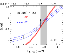
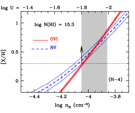
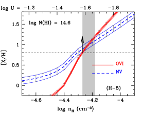
Figure 5.— PI models for the high-ionization absorption components, H–3 (left panel), H–4 (middle panel), and H–5 (right panel). Metallicity required to reproduce the observed column densities of individual high-ions (O vi and N v) are plotted as a function of gas density. The $N(\mbox{H\,{\sc i}})$ values assumed by the models are mentioned in the plot (see Table 2). The ionization parameters ($\log U$) corresponding to different $n_{\rm H}$ values are labelled at the top of each panel. The shaded regions represent the range in $\log n_{\rm H}$ (or $\log U$) over which $N(\mbox{O\,{\sc vi}})$ and $N(\mbox{N\,{\sc v}})$ match with our measurements. The horizontal dotted line represents the lower limit in metallicity indicated by the arrow.

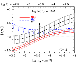
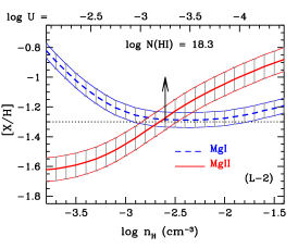
Figure 6.— Same as Figure 5 but for the low-ionization absorption components, L–1 (left panel), L–2 (middle panel), and L–3 (right panel). The measured $N(\mbox{Mg\,{\sc ii}})$ and $N(\mbox{Mg\,{\sc i}})$ values along with the $N(\mbox{H\,{\sc i}})$ limits are used to constrain the model parameters. As Mg i is not detected in L–1, $N(\mbox{C\,{\sc ii}})$ is used instead.

Appendix B Ionization Models: component-by-component

B.1. PI models for the high-ions

Here, we model the three high-ionization components (H–3, H–4, and H–5) in which both O vi and N v are positively detected and their column densities are well measured. As demonstrated in the previous section, the $N(\mbox{H\,{\sc i}})$ limits in H–3 and H–5 are also robust. For each of these components we compute ionization fractions for different species as a function of density for a given input metallicity using the corresponding $N(\mbox{H\,{\sc i}})$ limits as the stopping criterion for cloudy. In order to explore possible dependence of ionization fractions on the input metallicity, models were run for a series of different input metallicities (e.g. ${\rm[X/H]}=$ $-$1.0, 0.0, 0.3, 0.7, and 1.0). We, however, find that the ionization fractions do not show any significant dependence on the input metallicity in the optically thin regime for $\rm[X/H]<0.3$ for the entire density range of interest. For the components with derived metallicity $\rm[X/H]>0.3$, we use the cloudy model for which input metallicity is close to the derived metallicity. Using the model predicted ionization fractions and the observed column densities we determine loci of O vi and N v in the density–metallicity ($\log n_{\rm H}-{\rm[X/H]}$) plane.

In different panels of Figure 5, these loci of O vi and N v are shown. The curve corresponding to each ion (O vi or N v) represents the required metallicity to reproduce the observed column density as a function of $\log n_{\rm H}$ (or $\log U$). The range in $\rm[X/H]$ and in $\log n_{\rm H}$ for which both the curves overlap, represent a PI equilibrium solution since both $N(\mbox{O\,{\sc vi}})$ and $N(\mbox{N\,{\sc v}})$ are simultaneously reproduced.

In Table LABEL:tab_PIhigh we summarize the PI model solutions for the three high-ionization components. Densities as estimated for different components are consistent within $\sim 0.4$ dex with a median value of $n_{\rm H}\sim 10^{-4.2}$ cm^-3 (i.e. $\log U=-1.65$). The most interesting aspect of our models is to note the conservative lower limits on gas phase metallicities. All three components show super-solar metallicities with $\rm[X/H]\gtrsim 0.3$. For the H–3 and H–5 components, in which the $N(\mbox{H\,{\sc i}})$ limits are well constrained, the lower limits turn out to be $\rm[X/H]\gtrsim 0.6$ and $\rm[X/H]\gtrsim 0.7$, respectively. These metallicities are very high and very rare for any intervening absorption system. Such super-solar metallicities, however, is common in intrinsic QSO absorbers (e.g. Petitjean et al., 1994; Wu et al., 2010; Muzahid et al., 2013) that stem from the black hole accretion disk-wind. The total hydrogen column density is in the range $\log N_{\rm H}=17.8-18.6$ and the line-of-sight thickness range from 4 – 10 kpc. Note that the PI solutions for the high-ionization components did not produce any considerable column densities for the low-ions (e.g. C ii, Si ii, Si iii) but produced strong C iii, C iv, and moderate Si iv column densities. Finally, we find that the PI modeling for the H–1 and H–2 components, in which N v is not detected, suggest $\log n_{\rm H}<-4.1$ and $\rm[X/H]\lesssim 0.0$.

Table 5Photoionization model parameters for the high-ionization absorption components.

Component	$\log n_{\rm H}^{a}$	$\log U$	$\gtrsim{\rm[X/H]}^{a}$	$>\log N_{\rm H}$	$>L_{\rm los}$	$\log T$	Predicted $\log N$ (cm-2)
	(cm-3)			(cm-2)	(kpc)	(K)	N ii	Si ii	Si iii	C ii	C iii	C iv	S iv
(1)	(2)	(3)	(4)	(5)	(6)	(7)	(8)	(9)	(10)	(11)	(12)	(13)	(14)
H–3	$[-4.25$, $-4.15]$, ($-4.20$)	$[-1.70$, $-1.60]$	0.60, (0.8)	18.1	6	3.7	11.8	10.8	12.2	12.9	14.7	14.8	13.2
H–4	$[-4.05$, $-3.85]$, ($-3.95$)	$[-2.00$, $-1.80]$	0.30, (0.6)	18.6	10	4.0	12.3	11.4	12.8	13.3	15.0	15.1	13.7
H–5	$[-4.35$, $-4.25]$, ($-4.30$)	$[-1.60$, $-1.50]$	0.70, (0.9)	17.8	4	4.5	11.6	10.9	12.1	12.9	14.6	14.6	13.1

Note– ^aValues in the parenthesis are used to compute column densities in columns 8 through 14.

Table 6Photoionization model parameters for the low-ionization absorption components.

Component	$\log n_{\rm H}$	$\log U$	$\gtrsim{\rm[X/H]}^{a}$	$>\log N_{\rm H}$	$>L_{\rm los}$	$\log T$	Predicted $\log N$ (cm-2)
	(cm-3)			(cm-2)	(kpc)	(K)	N ii	Si ii	Si iii	C ii	C iii	Ca ii	Fe ii
(1)	(2)	(3)	(4)	(5)	(6)	(7)	(8)	(9)	(10)	(11)	(12)	(13)	(14)
L–1	$-2.40$	$-3.45$	$-2.00$	19.7	4	4.1	13.3	12.9	12.8	13.9a	13.8	11.1	12.6
L–2	$-2.60$	$-3.25$	$-1.30$	19.8	8	4.1	14.1	13.6	13.8	14.5	14.8	11.7	13.1
L–3	$-2.50$	$-3.35$	$-1.40$	19.7	5	4.1	13.9	13.4	13.5	14.3	14.5	11.6	13.0

Note– ^aC ii is used for constraining the model.

B.2. PI models for the low-ions

In Section III.1 we have demonstrated that the kinematics of O vi and Mg ii absorption are significantly different which indicate the multiphase structure of the absorber. In the previous section, we have shown that the gas phase that gives rise to O vi and N v under PI equilibrium cannot produce any considerable low-ions column densities. This further reinforces the idea of multiphase nature of the absorbing gas. To constrain the ionization parameters and chemical abundances in the low-ionization absorption components we have used the observed column densities of $N(\mbox{Mg\,{\sc i}})$ and $N(\mbox{Mg\,{\sc ii}})$ and the upper limits on $N(\mbox{H\,{\sc i}})$. Note that, as Mg i is not detected, $N(\mbox{C\,{\sc ii}})$ is used for constraining the model parameters for the L–1 component.

PI models for the low-ionization components L–1, L–2, and L–3 are shown in Figure 6 and the model parameters are summarized in Table LABEL:tab_PIlow. The densities in all these components are very similar (i.e. $n_{\rm H}\sim 10^{-2.5\pm 0.1}$  cm^-3). The metallicity in the L–1 component is ${\rm[X/H]}\gtrsim-2$, but it is roughly $\sim 0.7$ dex higher for the L–2 and L–3 components. It is interesting to note that while for the high-ionization components with detected N v, data do not allow a metallicity of $\rm[X/H]<0.3$, the low-ionization components can have significantly lower metallicities. However the metallicity need not necessarily be this low. Here, we have placed a very conservative lower limit on metallicity. The total hydrogen column densities in these components (i.e. $\log N_{\rm H}\sim 19.7-19.8$) are $\gtrsim 10$ times higher than what we have found for the high-ionization components (see Table LABEL:tab_PIhigh). The line-of-sight thicknesses of 4–8 kpc are, however, comparable to those of the high-ionization components. Note that our low-ionization phase solutions do not produce any appreciable amount of Si iv, C iv or any other higher ions (i.e. $\log N<13.0$). The model predicted column densities for different low-ions are presented in columns 8 through 14 of Table LABEL:tab_PIlow. We use these column densities to generate synthetic profiles using vpfit assuming pure non-thermal broadening. The synthetic profiles are shown in magenta curves in Figure 1. Note that these synthetic profiles explain the observed data adequately for C ii, N ii, Si ii, and Si iii. Our models, however, predict 0.3 and 0.5 dex higher Ca ii column densities in L–2 and L–4 components, respectively. It is known that Ca easily depletes on to dust. To be consistent with the data our PI model solutions would require a maximum of 0.5 dex depletion for calcium. Further, we note that our model predicted $N(\mbox{Fe\,{\sc ii}})$ values are 0.4 dex higher as compared to the measured values in the L–2 and L–3 components. This can be understood in terms of $\alpha$-enhancement. Note that, although we have built very reasonable PI models, the metallicity of the low-ionization components (L–2 and L–3 in particular) are not very well constrained due to the lack of higher order Lyman series lines. Spectral coverage of higher order Lyman-series lines down to the Lyman limit will be very useful in order to estimate metallicities in different low-ionization components accurately. Nevertheless, the metallicity of the L–1 component cannot be considerably higher than $\rm[X/H]=-2.0$, in order to explain the red wing of the Ly$\alpha$ profile.

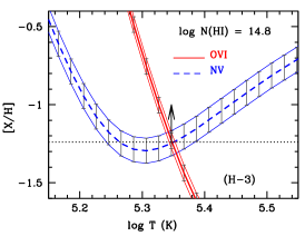
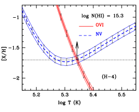
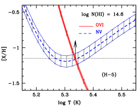
Figure 7.— CIE models for the high-ionization absorption components, H–3 (left panel), H–4 (middle panel), and H–5 (right panel). In each panel, different curves represent required metallicities to reproduce observed column densities for different high-ions (O vi and N v) as a function of gas temperature. The $N(\mbox{H\,{\sc i}})$ values assumed by the models are mentioned in the plot (see Table 2). The region in which the two curves overlap represents a CIE solution. It is evident that for all three components the required gas temperature is $\log T>5.3$, in order to reproduce the observed $N(\mbox{O\,{\sc vi}})$ and $N(\mbox{N\,{\sc v}})$ simultaneously. The arrow indicates the lower limit on metallicity in each panel.

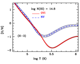
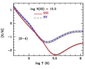
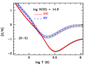
Figure 8.— Non-CIE isobaric cooling models for the high-ionization absorption components. Everything else is same as in Figure 7. It is evident that the observed $N(\mbox{O\,{\sc vi}})$ and $N(\mbox{N\,{\sc v}})$ can be reproduced simultaneously for gas temperature in the range $\log T\simeq 5.1-5.2$.

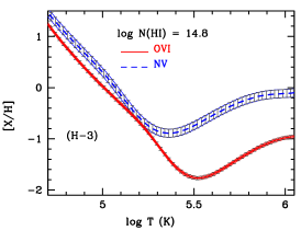
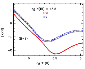
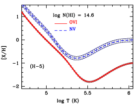
Figure 9.— Non-CIE isochoric cooling models for the high-ionization absorption components. Everything else is same as in Figure 7. It is apparent that the observed $N(\mbox{O\,{\sc vi}})$ and $N(\mbox{N\,{\sc v}})$ are not reproduced simultaneously for any of the components for the entire parameter space indicating no non-CIE solution.

B.3. CIE models for the high-ions

In this section we will explore the viability of CIE models for the high-ions. CIE models for the H–3, H–4, and H–5 components, in which N v is positively detected, are shown in Figure 7. We adopt the CIE models of Gnat & Sternberg (2007). In their models, equilibrium and non-equilibrium cooling efficiencies and ionization states for low-density radiatively cooling gas are computed under the assumption that the gas is dust-free, optically thin, and subject to no external radiation field. In each panels of Figure 7, we plot the metallicity required to produce the observed $N(\mbox{O\,{\sc vi}})$ and $N(\mbox{N\,{\sc v}})$ as a function of gas temperature ($\log T$) under CIE conditions. It is apparent from the figure that the observed $N(\mbox{O\,{\sc vi}})$ and $N(\mbox{N\,{\sc v}})$ are simultaneously explained for gas temperature in the range, $\log T\gtrsim 5.3-5.4$. The lower limit on metallicity for the H–3 and H–5 components, in which $N(\mbox{H\,{\sc i}})$ values are robustly constrained, turns out to be $\rm[X/H]>-1.2$ and for the H–4 component, $\rm[X/H]>-1.7$. Therefore, in contrast to the PI models, the gas-phase metallicity can be significantly lower under CIE conditions provided the gas temperature is $\log T\gtrsim 5.3$. Such a high temperature corresponds to a H i Doppler parameter of $b(\mbox{H\,{\sc i}})\gtrsim 57$ km s^-1. However, this large $b(\mbox{H\,{\sc i}})$ value, as suggested by the CIE models, is not supported by the COS data. As mentioned earlier in Appendix A a free fit to the non-black absorption seen in the Ly$\beta$ profile at $v\sim+100$ km s^-1 (i.e. the H–3 component) gives $b(\mbox{H\,{\sc i}})=28\pm 4$ km s^-1. This is half of the $b(\mbox{H\,{\sc i}})$ value required by the CIE models. Furthermore, we find that the CIE solutions do not produce any considerable $N(\mbox{C\,{\sc iv}})$ in any of the components. The maximum $N(\mbox{C\,{\sc iv}})$ predicted by our CIE model is $\log N=13.9$. However, in the low resolution $HST/$FOS spectrum, Chen et al. (2001) have detected a very strong C iv absorption from this system with $W_{r}=1.70$ Å. For comparison, the measured rest-frame equivalent width of O vi $\lambda 1031$ absorption is $W_{r}=1.02\pm 0.02$ Å. Therefore, the C iv is even stronger than the O vi in this system, since the $f\lambda$ value for the C iv $\lambda 1548$ transition is $\gtrsim 2$ times higher than that of O vi $\lambda 1031$. Nonetheless, CIE models fail to reproduce strong enough C iv along with N v and O vi. These facts indicate that a pure CIE model is not viable. Photoionization models (Appendix B.1), however, can reproduce strong C iv along with N v and O vi from a single gas phase.

B.4. Non-CIE models for the high ions

In this section, we investigate if non-CIE models can explain the high-ionization absorption components. Note that non-equilibrium effects become important in metal-rich environments when cooling efficiencies are increased and gas can cool faster than it recombines. Here, we consider two different non-CIE models of Gnat & Sternberg (2007), namely, isochoric (constant density) and isobaric (constant pressure) models. As discussed by the authors, isobaric cooling is less rapid compared to isochoric cooling and departures from equilibrium are somewhat smaller. Moreover, cooling that is initially isobaric eventually transforms to isochoric cooling (see their Figure 1).

In Figure 8 we show non-CIE isobaric cooling models for the H–3, H–4, and H–5 components. Clearly, these models suggest a gas temperature (e.g. $\log T\simeq 5.1-5.2$) which is only slightly lower than that predicted by the pure CIE models (see Figure 7). Note that for the H–3 component, the observed $N(\mbox{O\,{\sc vi}})/N(\mbox{N\,{\sc v}})$ ratio is consistent for a large range in gas temperature (i.e. $\log T\sim 4.7-5.3$). The lower limit on metallicity for $\log T\sim 5.3$ is $\rm[X/H]>-1.0$. The required metallicity sharply increases as the gas temperature decreases. For example, any temperature lower than $10^{5.1}$ K would require a super-solar metallicity. We note that for $\log T<5.1$ our model overproduces $N(\mbox{S\,{\sc iv}})$ by $\sim 0.4$ dex. Moreover, a temperature of $\log T\lesssim{4.8}$ overproduces $N(\mbox{Si\,{\sc iii}})$ by $\sim 2$ dex. We, thus, rule out the possibility of a gas temperature lower than $10^{5.1}$ K. Unlike CIE models, an isobaric cooling model solution with $\rm[X/H]\sim 0.0$ and $\log T\sim 5.1$ can produce a large C iv column density (e.g. $\log N>15.1$). Nonetheless, as discussed in the previous section, the $b$-parameter required for such a high temperature (i.e. $b(\mbox{H\,{\sc i}})>46$ km s^-1) is not supported by the Ly$\beta$ profile.

In Figure 9 we show non-CIE isochoric cooling models for the H–3, H–4, and H–5 components. Note that we do not find any possible solution that could explain the observed $N(\mbox{O\,{\sc vi}})$ and $N(\mbox{N\,{\sc v}})$ simultaneously within a $1\sigma$ measurement uncertainty. This clearly indicates that a non-CIE isochoric cooling model is not feasible. However, within $2\sigma$ allowed uncertainties we can have solutions which can be, again, ruled out by the arguments that were used previously to rule out the isobaric models.

Appendix C Equations for outflow energetics

In all the following equations: $r$ is the thin-shell radius, $\Delta r$ is the cloud thickness, $v_{w}$ is the outflow speed, $T$ is the cloud temperature, $N_{\rm H}$ is the total hydrogen column density, $C_{\Omega}$ is the global covering factor, $C_{f}$ is the local covering factor, $t_{\rm flow}$ is the flow time, $t_{\rm sound}$ is the sound crossing time, $M_{\rm out}$ is the mass carried by the thin-shell, $\dot{M}_{\rm out}$ is the mass-flow rate, and $\dot{E}_{k}$ is the kinetic luminosity. All other symbols have their usual meanings. We refer the reader Rupke et al. (2005) for detailed derivations of the Equations C3, C4, and C5.

$$\footnotesize t_{\rm flow}=5\times 10^{8}~{}{\rm yrs}\left(\frac{r}{100~{}{\rm kpc}}\right)\left(\frac{v_{w}}{200~{}{\rm kms^{-1}}}\right)^{-1}$$ (C1)

$$\footnotesize t_{\rm sound}=8\times 10^{8}~{}{\rm yrs}\left(\frac{\Delta r}{10~{}{\rm kpc}}\right)\left(\frac{T}{10^{4}~{}{\rm K}}\right)^{-\frac{1}{2}}$$ (C2)

$$\footnotesize\begin{split}M_{\rm out}&=4\pi\mu m_{p}C_{\Omega}C_{f}N_{\rm H}r^{2}=5.6\times 10^{10}M_{\odot}\\ &\times\left(\frac{C_{\Omega}}{0.4}C_{f}\right)\left(\frac{N_{\rm H}}{10^{20}~{}{\rm cm^{-2}}}\right)\left(\frac{r}{100~{}{\rm kpc}}\right)^{2}\end{split}$$ (C3)

$$\footnotesize\begin{split}{\dot{M}}_{\rm out}&=8\pi\mu m_{p}C_{\Omega}C_{f}N_{\rm H}rv_{w}=230~{}M_{\odot}~{}{\rm yr^{-1}}\\ &\times\left(\frac{C_{\Omega}}{0.4}C_{f}\right)\left(\frac{N_{\rm H}}{10^{20}~{}{\rm cm^{-2}}}\right)\left(\frac{r}{100~{}{\rm kpc}}\right)\left(\frac{v_{w}}{200~{}{\rm kms^{-1}}}\right)\end{split}$$ (C4)

$$\footnotesize\begin{split}{\dot{E}_{k}}&=\frac{1}{2}{\dot{M}}{v_{w}}^{2}=4\pi\mu m_{p}C_{\Omega}C_{f}N_{\rm H}r{v_{w}}^{3}=2.9\times 10^{42}~{}{\rm erg~{}s^{-1}}\\ &\times\left(\frac{C_{\Omega}}{0.4}C_{f}\right)\left(\frac{N_{\rm H}}{10^{20}~{}{\rm cm^{-2}}}\right)\left(\frac{r}{100~{}{\rm kpc}}\right)\left(\frac{v_{w}}{200~{}{\rm kms^{-1}}}\right)^{3}\end{split}$$ (C5)

References

- Adelberger et al. (2005) Adelberger, K. L., Shapley, A. E., Steidel, C. C., et al. 2005, ApJ, 629, 636
- Adelberger et al. (2003) Adelberger, K. L., Steidel, C. C., Shapley, A. E., & Pettini, M. 2003, ApJ, 584, 45
- Asplund et al. (2009) Asplund, M., Grevesse, N., Sauval, A. J., & Scott, P. 2009, ARA&A, 47, 481
- Baldwin et al. (1981) Baldwin, J. A., Phillips, M. M., & Terlevich, R. 1981, PASP, 93, 5
- Bertin & Arnouts (1996) Bertin, E., & Arnouts, S. 1996, A&AS, 117, 393
- Bolzonella et al. (2000) Bolzonella, M., Miralles, J.-M., & Pelló, R. 2000, A&A, 363, 476
- Bordoloi et al. (2011) Bordoloi, R., Lilly, S. J., Knobel, C., et al. 2011, ApJ, 743, 10
- Bordoloi et al. (2014a) Bordoloi, R., Tumlinson, J., Werk, J. K., et al. 2014a, ApJ, 796, 136
- Bordoloi et al. (2014b) Bordoloi, R., Lilly, S. J., Hardmeier, E., et al. 2014b, ApJ, 794, 130
- Borthakur et al. (2015) Borthakur, S., Heckman, T. M., Tumlinson, J., et al. 2015, ArXiv e-prints, arXiv:1504.01392
- Bouché et al. (2012) Bouché, N., Hohensee, W., Vargas, R., et al. 2012, MNRAS, 426, 801
- Bryan & Norman (1998) Bryan, G. L., & Norman, M. L. 1998, ApJ, 495, 80
- Chen et al. (2001) Chen, H.-W., Lanzetta, K. M., Webb, J. K., & Barcons, X. 2001, ApJ, 559, 654
- Chen & Mulchaey (2009) Chen, H.-W., & Mulchaey, J. S. 2009, ApJ, 701, 1219
- Churchill & Charlton (1999) Churchill, C. W., & Charlton, J. C. 1999, AJ, 118, 59
- Churchill et al. (2000) Churchill, C. W., Mellon, R. R., Charlton, J. C., et al. 2000, ApJS, 130, 91
- Churchill et al. (2013a) Churchill, C. W., Nielsen, N. M., Kacprzak, G. G., & Trujillo-Gomez, S. 2013a, ApJ, 763, L42
- Churchill et al. (2013b) Churchill, C. W., Trujillo-Gomez, S., Nielsen, N. M., & Kacprzak, G. G. 2013b, ApJ, 779, 87
- Coleman et al. (1980) Coleman, G. D., Wu, C.-C., & Weedman, D. W. 1980, ApJS, 43, 393
- Danforth et al. (2010) Danforth, C. W., Stocke, J. T., & Shull, J. M. 2010, ApJ, 710, 613
- Davé et al. (2011a) Davé, R., Finlator, K., & Oppenheimer, B. D. 2011a, MNRAS, 416, 1354
- Davé et al. (2012) —. 2012, MNRAS, 421, 98
- Davé et al. (2011b) Davé, R., Oppenheimer, B. D., & Finlator, K. 2011b, MNRAS, 415, 11
- Dekel & Birnboim (2006) Dekel, A., & Birnboim, Y. 2006, MNRAS, 368, 2
- Dekel et al. (2009) Dekel, A., Birnboim, Y., Engel, G., et al. 2009, Nature, 457, 451
- Dekker et al. (2000) Dekker, H., D’Odorico, S., Kaufer, A., Delabre, B., & Kotzlowski, H. 2000, in Proc. SPIE, 4008, 534-545
- Ding et al. (2003) Ding, J., Charlton, J. C., Churchill, C. W., & Palma, C. 2003, ApJ, 590, 746
- Faber et al. (2007) Faber, S. M., Willmer, C. N. A., Wolf, C., et al. 2007, ApJ, 665, 265
- Fechner & Richter (2009) Fechner, C., & Richter, P. 2009, A&A, 496, 31
- Ferland et al. (2013) Ferland, G. J., Porter, R. L., van Hoof, P. A. M., et al. 2013, Rev. Mexicana Astron. Astrofis., 49, 137
- Ford et al. (2014) Ford, A. B., Davé, R., Oppenheimer, B. D., et al. 2014, MNRAS, 444, 1260
- Fox et al. (2007) Fox, A. J., Petitjean, P., Ledoux, C., & Srianand, R. 2007, A&A, 465, 171
- Fox et al. (2013) Fox, A. J., Lehner, N., Tumlinson, J., et al. 2013, ApJ, 778, 187
- Fox et al. (2015) Fox, A. J., Bordoloi, R., Savage, B. D., et al. 2015, ApJ, 799, L7
- Ghavamian et al. (2009) Ghavamian, P., Aloisi, A., Lennon, D., et al. 2009, Preliminary Characterization of the Post- Launch Line Spread Function of COS, Tech. rep.
- Gnat & Sternberg (2007) Gnat, O., & Sternberg, A. 2007, ApJS, 168, 213
- Green et al. (2012) Green, J. C., Froning, C. S., Osterman, S., et al. 2012, ApJ, 744, 60
- Grimes et al. (2009) Grimes, J. P., Heckman, T., Aloisi, A., et al. 2009, ApJS, 181, 272
- Haardt & Madau (1996) Haardt, F., & Madau, P. 1996, ApJ, 461, 20
- Haardt & Madau (2012) —. 2012, ApJ, 746, 125
- Hamann & Ferland (1999) Hamann, F., & Ferland, G. 1999, ARA&A, 37, 487
- Hamann et al. (2000) Hamann, F. W., Netzer, H., & Shields, J. C. 2000, ApJ, 536, 101
- Hao et al. (2011) Hao, C.-N., Kennicutt, R. C., Johnson, B. D., et al. 2011, ApJ, 741, 124
- Heckman (2003) Heckman, T. M. 2003, in Revista Mexicana de Astronomia y Astrofisica, vol. 27, Vol. 17, Revista Mexicana de Astronomia y Astrofisica Conference Series, ed. V. Avila-Reese, C. Firmani, C. S. Frenk, & C. Allen, 47–55
- Hussain et al. (2015) Hussain, T., Muzahid, S., Narayanan, A., et al. 2015, MNRAS, 446, 2444
- Kacprzak et al. (2010) Kacprzak, G. G., Churchill, C. W., Ceverino, D., et al. 2010, ApJ, 711, 533
- Kacprzak et al. (2011) Kacprzak, G. G., Churchill, C. W., Evans, J. L., Murphy, M. T., & Steidel, C. C. 2011, MNRAS, 416, 3118
- Kacprzak et al. (2012) Kacprzak, G. G., Churchill, C. W., & Nielsen, N. M. 2012, ApJ, 760, L7
- Kacprzak et al. (2008) Kacprzak, G. G., Churchill, C. W., Steidel, C. C., & Murphy, M. T. 2008, AJ, 135, 922
- Kacprzak et al. (2014) Kacprzak, G. G., Martin, C. L., Bouché, N., et al. 2014, ApJ, 792, L12
- Kereš et al. (2009) Kereš, D., Katz, N., Fardal, M., Davé, R., & Weinberg, D. H. 2009, MNRAS, 395, 160
- Kereš et al. (2005) Kereš, D., Katz, N., Weinberg, D. H., & Davé, R. 2005, MNRAS, 363, 2
- Khaire & Srianand (2015) Khaire, V., & Srianand, R. 2015, MNRAS, 451, L30
- Kim et al. (1996) Kim, A., Goobar, A., & Perlmutter, S. 1996, PASP, 108, 190
- Klypin et al. (2011) Klypin, A. A., Trujillo-Gomez, S., & Primack, J. 2011, ApJ, 740, 102
- Kriss (2011) Kriss, G. A. 2011, Improved Medium Resolution Line Spread Functions for COS FUV Spectra, Tech. rep.
- Lehner et al. (2014) Lehner, N., O’Meara, J. M., Fox, A. J., et al. 2014, ApJ, 788, 119
- Lehner et al. (2009) Lehner, N., Prochaska, J. X., Kobulnicky, H. A., et al. 2009, ApJ, 694, 734
- Lehner et al. (2013) Lehner, N., Howk, J. C., Tripp, T. M., et al. 2013, ApJ, 770, 138
- Martin (2005) Martin, C. L. 2005, ApJ, 621, 227
- Mathes et al. (2014) Mathes, N. L., Churchill, C. W., Kacprzak, G. G., et al. 2014, ApJ, 792, 128
- Misawa et al. (2007) Misawa, T., Charlton, J. C., Eracleous, M., et al. 2007, ApJS, 171, 1
- Morton (2003) Morton, D. C. 2003, ApJS, 149, 205
- Muzahid (2014) Muzahid, S. 2014, ApJ, 784, 5
- Muzahid et al. (2013) Muzahid, S., Srianand, R., Arav, N., Savage, B. D., & Narayanan, A. 2013, MNRAS, 431, 2885
- Muzahid et al. (2012) Muzahid, S., Srianand, R., Bergeron, J., & Petitjean, P. 2012, MNRAS, 421, 446
- Narayanan et al. (2010) Narayanan, A., Savage, B. D., & Wakker, B. P. 2010, ApJ, 712, 1443
- Nielsen et al. (2013a) Nielsen, N. M., Churchill, C. W., & Kacprzak, G. G. 2013a, ApJ, 776, 115
- Nielsen et al. (2015) Nielsen, N. M., Churchill, C. W., Kacprzak, G. G., Murphy, M. M., & Evans, J. L. 2015, ArXiv e-prints, arXiv:1505.07167
- Nielsen et al. (2013b) Nielsen, N. M., Churchill, C. W., Kacprzak, G. G., & Murphy, M. T. 2013b, ApJ, 776, 114
- Oppenheimer et al. (2010) Oppenheimer, B. D., Davé, R., Kereš, D., et al. 2010, MNRAS, 406, 2325
- Osterman et al. (2011) Osterman, S., Green, J., Froning, C., et al. 2011, Ap&SS, 335, 257
- Petitjean et al. (1994) Petitjean, P., Rauch, M., & Carswell, R. F. 1994, A&A, 291, 29
- Pettini (2004) Pettini, M. 2004, in Cosmochemistry. The melting pot of the elements, ed. C. Esteban, R. García López, A. Herrero, & F. Sánchez, 257–298
- Pettini et al. (2008) Pettini, M., Zych, B. J., Steidel, C. C., & Chaffee, F. H. 2008, MNRAS, 385, 2011
- Prochaska et al. (2011) Prochaska, J. X., Weiner, B., Chen, H. ., Mulchaey, J. S., & Cooksey, K. L. 2011, ArXiv e-prints (astro-ph/1103.1891), arXiv:1103.1891
- Rubin et al. (2014) Rubin, K. H. R., Prochaska, J. X., Koo, D. C., et al. 2014, ApJ, 794, 156
- Rubin et al. (2010) Rubin, K. H. R., Weiner, B. J., Koo, D. C., et al. 2010, ApJ, 719, 1503
- Rupke et al. (2005) Rupke, D. S., Veilleux, S., & Sanders, D. B. 2005, ApJS, 160, 115
- Savage et al. (2014) Savage, B. D., Kim, T.-S., Wakker, B. P., et al. 2014, ApJS, 212, 8
- Savage et al. (2003) Savage, B. D., Sembach, K. R., Wakker, B. P., et al. 2003, ApJS, 146, 125
- Savage et al. (2010) Savage, B. D., Narayanan, A., Wakker, B. P., et al. 2010, ApJ, 719, 1526
- Schroetter et al. (2015) Schroetter, I., Bouché, N., Péroux, C., et al. 2015, ApJ, 804, 83
- Sembach et al. (2003) Sembach, K. R., Wakker, B. P., Savage, B. D., et al. 2003, ApJS, 146, 165
- Shapley et al. (2003) Shapley, A. E., Steidel, C. C., Pettini, M., & Adelberger, K. L. 2003, ApJ, 588, 65
- Sharma & Nath (2012) Sharma, M., & Nath, B. B. 2012, ApJ, 750, 55
- Sheinis et al. (2002) Sheinis, A. I., Bolte, M., Epps, H. W., et al. 2002, PASP, 114, 851
- Simard et al. (2002) Simard, L., Willmer, C. N. A., Vogt, N. P., et al. 2002, ApJS, 142, 1
- Springel & Hernquist (2003) Springel, V., & Hernquist, L. 2003, MNRAS, 339, 289
- Srianand et al. (2002) Srianand, R., Petitjean, P., Ledoux, C., & Hazard, C. 2002, MNRAS, 336, 753
- Steidel et al. (2002) Steidel, C. C., Kollmeier, J. A., Shapley, A. E., et al. 2002, ApJ, 570, 526
- Stocke et al. (2013) Stocke, J. T., Keeney, B. A., Danforth, C. W., et al. 2013, ApJ, 763, 148
- Thom et al. (2012) Thom, C., Tumlinson, J., Werk, J. K., et al. 2012, ApJ, 758, L41
- Tripp et al. (2008) Tripp, T. M., Sembach, K. R., Bowen, D. V., et al. 2008, ApJS, 177, 39
- Tripp et al. (2011) Tripp, T. M., Meiring, J. D., Prochaska, J. X., et al. 2011, Science, 334, 952
- Tumlinson et al. (2011a) Tumlinson, J., Werk, J. K., Thom, C., et al. 2011a, ApJ, 733, 111
- Tumlinson et al. (2011b) Tumlinson, J., Thom, C., Werk, J. K., et al. 2011b, Science, 334, 948
- van Zee & Haynes (2006) van Zee, L., & Haynes, M. P. 2006, ApJ, 636, 214
- van Zee et al. (1998) van Zee, L., Salzer, J. J., Haynes, M. P., O’Donoghue, A. A., & Balonek, T. J. 1998, AJ, 116, 2805
- Veilleux et al. (2005) Veilleux, S., Cecil, G., & Bland-Hawthorn, J. 2005, ARA&A, 43, 769
- Wakker et al. (2003) Wakker, B. P., Savage, B. D., Sembach, K. R., et al. 2003, ApJS, 146, 1
- Werk et al. (2013) Werk, J. K., Prochaska, J. X., Thom, C., et al. 2013, ApJS, 204, 17
- Werk et al. (2014) Werk, J. K., Prochaska, J. X., Tumlinson, J., et al. 2014, ApJ, 792, 8
- Wolf et al. (2003) Wolf, C., Meisenheimer, K., Rix, H.-W., et al. 2003, A&A, 401, 73
- Wu et al. (2010) Wu, J., Charlton, J. C., Misawa, T., Eracleous, M., & Ganguly, R. 2010, ApJ, 722, 997