$PT$-symmetric invisible defects and confluent Darboux-Crum transformations

Abstract

We show that confluent Darboux-Crum transformations with emergent Jordan states are an effective tool for the design of optical systems governed by the Helmholtz equation under the paraxial approximation. The construction of generic, asymptotically real and periodic, $PT$-symmetric systems with local complex periodicity defects is discussed in detail. We show how the decay rate of the defect is related with the energy of the bound state trapped by the defect. In particular, the bound states in the continuum are confined by the periodicity defects with power law decay. We show that these defects possess complete invisibility; the wave functions of the system coincide asymptotically with the wave functions of the undistorted setting. The general results are illustrated with explicit examples of reflectionless models and systems with one spectral gap. We show that the spectral properties of the studied models are reflected by Lax-Novikov-type integrals of motion and associated supersymmetric structures of bosonized and exotic nature.

1 Introduction

Propagation of light beams can mimic evolution of matter waves in quantum systems. This follows from the formal coincidence of the Helmholtz equation for monochromatic light, propagating in magnetization free medium, and the stationary Schrödinger equation in quantum mechanics [1]. In this manner, behavior of quantum systems can be simulated by optical systems, and, vice versa, concepts common in optics can find their way to quantum settings.

Nowadays, there can be constructed optical materials where intensity of light is subject to a controlled gain and loss [2], [3], [4]. Unusual optical properties of these systems are reflected by refractive index that acquires complex values. The perfect match between gain and loss prevents the light from being exponentially dimmed or brightened and it is reflected by invariance of the refractive index with respect to combined transformations of space-inversion ($P$) and time-reversal ($T$). The light passing through such a material can exhibit some remarkable properties. Among them, let us mention power oscillations or non-reciprocity of beam propagation that are caused by non-orthogonality of Bloch states [5], [6], [7], [8], [9], violation of Friedel’s law of Bragg scattering [10], unidirectional invisibility [11], [12], [13], [14] or invisibility of defects in the periodic structure of optical crystals [15], [16].

The peculiar features of the $PT$-symmetric optical systems can be captured by the Helmholtz (Schrödinger) equation with a non-hermitian Hamiltonian. Such Hamiltonian operators have been studied extensively in quantum mechanics for last two decades, see [17], [18], [19] for review. It was understood that reality of their spectra occurs due to existence of an antilinear integral of motion that was identified with the $PT$ operator in most cases. The lack of hermiticity of the energy operator challenges probability interpretation for a quantum system; the scalar product has to be redefined [20]-[22] and its explicit form is usually exceedingly difficult to find.

As the solutions of the Helmholtz equation correspond to a purely classical object (amplitude of the electric field), the hassle of the probability interpretation is avoided. In fact, the optical systems with balanced gain and loss open the door for realization of interesting phenomena predicted by non-Hermitian ($PT$-symmetric) quantum mechanics. One of them corresponds to the transition between exact and spontaneously broken $PT$ symmetry, where the behavior of a physical system at the vicinity of the exceptional spectral points was of the main interest [23], [10], [24].

The Helmholtz equation for linearly polarized light acquires the form

$$\left(\partial_{z}^{2}+\partial_{x}^{2}+\frac{n^{2}(x)}{c^{2}}\omega^{2}\right)\Psi(x,z)=0,$$ (1.1)

where $\omega$ is the frequency of monochromatic beam, and $\Psi$ is electric field. The refractive index $n(x)=n_{0}+\delta n(x)$, where $n_{0}>0$ and $|\delta n(x)|<<n_{0}$, is $PT$ symmetric, i.e. $\delta n(x)={\delta n(-x)}^{*}$. In dependence of its sign, the imaginary part of $\delta n(x)$ represents loss or gain. In the paraxial approximation, we set $\Psi(x,z)=e^{i\frac{n_{0}\omega}{c}z}\psi(x,z)$, where $\psi(x,z)$ is an envelope function slowly varying in $z$. Neglecting the term with $\partial_{z}^{2}\psi$, the Helmholtz equation reduces then to

$$i\partial_{z}\psi(x,z)=[-\partial_{x}^{2}+V(x)]\psi(x,z),$$ (1.2)

where $z$ denotes a depth of propagation of light in the crystal while $x$ is a transverse coordinate. The potential $V(x)$ is proportional to $\delta n(x)$, $V(x)\sim\delta n(x)$. The form of physically acceptable solutions of (1.2) depends on characteristics of the considered system; they can be square integrable in $x$, or quasi-periodic in $x$ when $V(x)$ is a periodic function. It is worth stressing that contrary to the $PT$-symmetric quantum mechanics, the quantity $\mathcal{P}(z)=\int_{-\infty}^{\infty}|\psi(x,z)|^{2}dx$ is physically relevant as it denotes the power of the beam $\psi(x,z)$ when measured in the depth $z$ within the crystal. Due to the complex refractive index, the power $\mathcal{P}(z)$ can be oscillating function in $z$ as the beam propagates though the medium, see e.g. [6].

In the current article, we will have in mind primarily the framework of paraxial approximation described by (1.2), suitable for the low frequencies where the term $\partial_{z}^{2}\psi$ can be neglected. Let us notice that another situation is also of interest in the literature, where no paraxial approximation is employed [11], [13]. By separation of variables $\Psi(x,z)=e^{i\lambda z}\psi(x)$, the equation (1.1) reduces effectively to $\left(\frac{d^{2}}{dx^{2}}+\frac{n^{2}(x)}{c^{2}}\omega^{2}-\lambda^{2}\right)\psi(x)=0.$ Here, the inhomogeneities of refractive index are developed in the direction of propagation of light, contrary to (1.2) where the light propagates in normal direction to the inhomogeneities of $n(x)$. Our results will be applicable in this scheme as well.

Supersymmetric quantum mechanics (SUSYQM) provides powerful techniques for construction and analysis of quantum systems. It allows us to alter interaction terms of both exactly- and quasi-exactly solvable models without compromising their solvability properties. It relates the scattering characteristics such as reflection and transmission amplitudes of the two systems [26]. It can serve to find integrals of motion of the new systems; in the case of finite-gap and reflectionless systems, the nontrivial (Lax-Novikov) integrals can be identified in straightforward manner [27, 28, 29, 30]. The framework of SUSYQM can also be used very efficiently in the analysis of the soliton scattering, or to construct (multi-)soliton solutions of Korteweg-de Vries (KdV) and modified Korteweg-de Vries equations proceeding from the trivial solutions, see e.g. [31], [32].

SUSYQM relies on the intertwining operators. These are frequently represented in terms of higher-order differential operators and identified as Darboux-Crum transformations known from the analysis of differential equations [33]. They are usually used to construct systems with altered number of discrete energies. Requirement of regularity of a new system imposes some restrictions to the use and setup of Darboux-Crum transformations. Discrete energies that lie below the spectral threshold of the original system can be added by the first order Darboux transformations. To generate discrete energy levels within a bounded gap separating the spectral bands of an original, periodic system, Darboux-Crum transformations of higher order have to be employed, see [35].

Methods of quantum mechanics provide efficient tools for analysis of optical systems. They have been used in the optics for a few decades [36]-[42]. In recent years, popularity of the supersymmetric approach witnesses growing interest in the context of the $PT$-symmetric optical devices [43]-[48]. It allows to construct solvable models of optical crystals with reflectionless interfaces [43], the systems possessing unidirectional invisibility [46], or periodic crystals with invisible periodicity defects [45].

Developing further the pioneering ideas of von Neumann and Wigner [49], a supersymmetric generalization of the procedure for the construction of spherically symmetric scattering potentials that support bound states in the continuum was proposed in Refs. [50], [51]. General aspects of the technique, known in the literature as confluent Darboux(-Crum) transformation, have been analyzed in the series of papers [52, 53, 54, 55, 56], see also refs. [57, 58]. The extension of the generalized framework to the systems defined on the whole real axis leads to the construction of non-Hermitian systems. Those were considered in the context of optics e.g. in [59], [60].

Bound states in the continuum (BIC) can be observed experimentally in optical systems [61] and their theoretical investigation in the context of $PT$-symmetric lattices was done, for instance, in refs. [62], [63]. The bound states located on the threshold of the continuum spectrum of PT symmetric systems were considered in [45].

In the present work, by a systematic employment of SUSYQM, we will construct $PT$-symmetric optical systems where the refraction index is asymptotically real and periodic, however, there are localized complex periodicity defects. We will show analytically that the decay rate of the defects is related to the energy of the bound states induced by them; the defects fall off as $x^{-1}$ or $x^{-2}$ for the systems with BIC, whereas exponential decay takes place for bound states associated with discrete energies.

The work is organized as follows. In the next section, we will present the main characteristics of the confluent Darboux-Crum transformations (also called double step Darboux transformations in the literature), the basic tool for construction of the systems with bound states in the continuum. We will explain its relation to the standard supersymmetric quantum mechanics and provide formulas for the bound states and potential of the new system. We will review basic properties of periodic systems in section 3, where we focus on the $PT$-symmetry of Bloch-Floquet states. In section 4, we will focus on the $PT$-symmetric potentials that support bound states in the continuum. Results of the systematic analysis are illustrated on the examples in section 5. We discuss there, particularly, reflectionless systems that possess either visible or invisible defects. We consider one-gap systems that possess bound states in the continuum as well. In section 6, we discuss some peculiar properties of reflectionless and finite-gap systems. In particular, we focus on the integrals of motion that reflect spectral properties of the systems manifested in two kinds of associated superalgebras. One of them corresponds to a hidden bosonized supersymmetry. It is based here on Lax-Novikov integrals mixed up with confluent Darboux-Crum transformations. The other one is an exotic hidden nonlinear supersymmetry based on the extended matrix Hamiltonian and containing the extended number of integrals of motion in comparison with a usual $N=2$ supersymmetric structure. The last section is devoted to discussion and outlook.

2 Confluent Darboux-Crum transformation and Jordan states

For any quantum system we obtain here a partner by employing a confluent Darboux-Crum transformation, and observe the emergence of the Jordan states in the construction. Such states will appear later in the structure of the Lax-Novikov integrals controlling the invisibility of the $PT$-symmetric defects.

Consider a quantum system given by the Schrödinger Hamiltonian

$$H=-\frac{d^{2}}{dx^{2}}+V(x)\,.$$ (2.1)

Let $\psi_{0}(x)$ be a (physical or non-physical) eigenstate of eigenvalue $E_{0}$,

$$(H-E_{0})\psi_{0}=0\,.$$ (2.2)

We use it to introduce the first order differential operators

$$A:=\psi_{0}\frac{d}{dx}\frac{1}{\psi_{0}}=\frac{d}{dx}-\frac{\psi_{0}^{\prime}}{\psi_{0}}\,,\qquad A^{\sharp}:=-\frac{1}{\psi_{0}}\frac{d}{dx}\psi_{0}=-\frac{d}{dx}-\frac{\psi_{0}^{\prime}}{\psi_{0}}\,.$$ (2.3)

By definition,

$$A\psi_{0}=0,\ \qquad A^{\sharp}\frac{1}{\psi_{0}}=0\,.$$ (2.4)

A linear independent from $\psi_{0}$ eigenstate of $H$ of the same eigenvalue $E_{0}$ we take in a form

$${\psi}_{0}{}^{\flat}(x)=\psi_{0}(x)\left(\int_{x_{0}}^{x}\frac{ds}{\psi^{2}_{0}(s)}+a\right)\,,\quad a\in\mathbb{C}\,,$$ (2.5)

where $x_{0}\in\mathbb{R}$ is some fixed point. Notice that the Wronskian $W(f,g):=fg^{\prime}-f^{\prime}g$ of $\psi_{0}$ and ${\psi_{0}}^{\flat}$ is unit, $W(\psi_{0},{\psi_{0}}^{\flat})=1$. In what follows by ${\psi}^{\flat}(x)$ we shall denote a function associated with a function $\psi(x)$ according to the rule (2.5).

The application of $A$ and $A^{\sharp}$ to $\psi_{0}{}^{\flat}$ and $(1/\psi_{0})^{\flat}$, respectively, gives

$$A{\psi_{0}}^{\flat}=\frac{1}{\psi_{0}},\qquad A^{\sharp}{\left(\frac{1}{\psi_{0}}\right)}^{\flat}=-\psi_{0}\,.$$ (2.6)

By virtue of Eqs. (2.4) and (2.6), the first order operators (2.3) factorize the shifted Hamiltonian,

$$H-E_{0}=A^{\sharp}A\,.$$ (2.7)

The alternative product of $A$ and $A^{\sharp}$ gives the shifted Darboux (SUSY) partner Hamiltonian $\breve{H}$,

$$\breve{H}-E_{0}=AA^{\sharp}=-\frac{d^{2}}{dx^{2}}+\breve{V}(x)\,,\quad{\rm with}\qquad\breve{V}(x)=V(x)-2\left(\log\psi_{0}(x))\right)^{\prime\prime}.$$ (2.8)

The nodes of $\psi_{0}$ give rise to singularities in $\breve{V}(x)$ not present in $V(x)$. When $\breve{V}(x)$ is required to inherit the regularity of $V(x)$, $\psi_{0}$ has to be fixed as a nodeless function. The intertwining relations

$$AH=\breve{H}A\,,\qquad A^{\sharp}\breve{H}=HA^{\sharp}\,,$$ (2.9)

follow then from (2.7) and (2.8). The operator $\breve{H}-E_{0}$ annihilates the states ${1}/{\psi_{0}}$ and ${\left({1}/{\psi_{0}}\right)^{\flat}}$.

In dependence on the nature of $E_{0}$ and $\psi_{0}(x)$, the Hamiltonians $H$ and $\breve{H}$ are isospectral or almost isospectral up to eigenvalue $E_{0}$, which can be present in one system but missing in the other one. Operators $A$ and $A^{\sharp}$ realize a mapping between two-dimensional eigenspaces of the second order differential operators $H$ and $\breve{H}$,

$$A\psi_{E}=\breve{\psi}_{E}\,,\qquad A^{\sharp}\breve{\psi}_{E}=(E-E_{0})\psi_{E}\,,$$ (2.10)

for any $E\neq E_{0}$ and corresponding eigenstates, $H\psi_{E}=E\psi_{E}$, $\breve{H}\breve{\psi}_{E}=E\breve{\psi}_{E}$.

Notice that the zero mode ${\psi_{0}}^{\flat}$ of $H-E_{0}$ is mapped by $A$ into the zero mode $1/\psi_{0}$ of $\breve{H}-E_{0}$ and, analogously, the zero mode ${(1/\psi_{0})}^{\flat}$ of $\breve{H}-E_{0}$ is mapped by $A^{\sharp}$ into the zero mode $\psi_{0}$ of $H-E_{0}$. However, the pre-image of the zero mode ${\psi_{0}}^{\flat}$ of $H-E_{0}$ with respect to the action of $A^{\sharp}$ is not a zero mode of $\breve{H}-E_{0}$. Similarly, the pre-image of the zero mode ${(1/\psi_{0})}^{\flat}$ of $\breve{H}-E_{0}$ under the action of $A$ does not belong to the kernel of $H-E_{0}$. Instead, the indicated pre-images are the Jordan states of the corresponding operators $H-E_{0}$ and $\breve{H}-E_{0}$. Indeed, consider the equation

$$A\chi=-{(1/\psi_{0})}^{\flat}\,.$$ (2.11)

Its solution is

$$\chi(x)=-\psi_{0}(x)\left(\int_{x_{0}}^{x}\frac{1}{\psi_{0}(s)}({1/\psi_{0}(s)})^{\flat}ds+a\right)=-\psi_{0}(x)\left(\int_{x_{0}}^{x}\frac{\alpha+\int_{x_{0}}^{s}\psi_{0}^{2}(r)dr}{\psi_{0}^{2}(s)}ds+a\right)\,,$$ (2.12)

where $a\in\mathbb{C}$ and $\alpha\in\mathbb{C}$ are some constants. Acting on both sides of (2.11) by $A^{\sharp}$, one finds that

$$(H-E_{0})\chi=\psi_{0}\,,\quad(H-E_{0})^{2}\chi=0\,.$$ (2.13)

This means that $\chi(x)$ is the Jordan state of $H-E_{0}$. Analogously, we find that the solution of equation $A^{\sharp}\lambda={\psi_{0}}^{\flat},$ given by $\lambda(x)=-\frac{1}{\psi_{0}(x)}\left(\int_{x_{0}}^{x}\psi_{0}(s){\psi_{0}}^{\flat}(s)ds+b\right)\,,\ b\in\mathbb{C}\,,$ satisfies $(\breve{H}-E_{0})\lambda={1}/{\psi_{0}}\,,$ $(\breve{H}-E_{0})^{2}\lambda=0$. Without loss of generality, we set below $a=0$ in (2.12).

Let us take $E\neq E_{0}$ and consider the eigenstate equation

$$(H-E)\Psi(x;E)=0\,.$$ (2.14)

We suppose that $E$ is sufficiently close to $E_{0}$ and denote $E-E_{0}=\varepsilon$. Assuming the analyticity of $\Psi(x;E)$ in $E$ in vicinity of $E_{0}$, we look for solution of (2.14) close to $\psi_{0}(x)$ in the form of the Taylor series in $\varepsilon$,

$$\Psi(x;E)=\psi_{0}(x)+\sum_{n=1}\frac{\varepsilon^{n}}{n!}\chi_{n}(x)\,,\qquad\chi_{n}(x)=\frac{\partial^{n}\Psi(x;E)}{\partial E^{n}}|_{E=E_{0}}.$$ (2.15)

Substituting this series into (2.14), we find that $\chi_{n}(x)$ are defined recursively by

$$(H-E_{0})\chi_{1}(x)=\psi_{0}(x)\,,$$ (2.16)

$$(H-E_{0})\chi_{n}(x)=n\chi_{n-1}(x)\,,\qquad n=2,\ldots.$$ (2.17)

Therefore, $\chi_{1}(x)$ is just the Jordan state that appeared in Eq. (2.13), $\chi_{1}(x)=\chi(x)$. The state $\chi_{n}(x)$ with $n\geq 2$ satisfies relations $(H-E_{0})^{n}\chi_{n}(x)=\psi_{0}(x)$, $(H-E_{0})^{n+1}\chi_{n}(x)=0$, and can be identified as a higher, $n$-th order Jordan state.

Consider the system $\tilde{H}_{\varepsilon}=-\frac{d^{2}}{dx^{2}}+V_{\varepsilon}(x)$ generated from $H$ by applying to the latter the Darboux-Crum transformation based on the eigenstates $\psi_{0}(x)$ and $\Psi(x;E)$,

$$V_{\varepsilon}(x)=V(x)-2\left(\log W(\psi_{0}(x),\Psi(x;E))\right)^{\prime\prime}\,.$$ (2.18)

Taking into account equation (2.15), in the limit $\varepsilon\rightarrow 0$ we get

$$\tilde{V}:=\lim_{\varepsilon\rightarrow 0}V_{\varepsilon}(x)=V(x)-2\left(\log W(\psi_{0}(x),\chi(x))\right)^{\prime\prime}.$$ (2.19)

Relation $W(f,g)=f^{2}\frac{d}{dx}(\frac{g}{f})$ together with Eq. (2.12) gives us

$$\tilde{V}(x) =V(x)-2\frac{d^{2}}{dx^{2}}\log\,\mathcal{I}(x)=V(x)-4\frac{\psi_{0}\psi_{0}^{\prime}}{\int_{0}^{x}\psi_{0}^{2}+\alpha}+2\frac{\psi_{0}^{4}}{\left(\int_{0}^{x}\psi_{0}^{2}+\alpha\right)^{2}}\,,$$ (2.20)

where

$$\mathcal{I}(x)=\int_{0}^{x}\psi_{0}^{2}(s)ds+\alpha\,,$$ (2.21)

and from now on we set $x_{0}=0$.

In correspondence with the Darboux-Crum construction, the Hamiltonian operators $H$, $\breve{H}$ and

$$\tilde{H}:=-\frac{d^{2}}{dx^{2}}+\tilde{V}$$ (2.22)

are almost isospectral. Since in the limit $\varepsilon\rightarrow 0$, $A\Psi(x;E_{0}+\varepsilon)=A(\psi_{0}+\varepsilon\chi)=\varepsilon A\chi=\varepsilon{(1/\psi_{0})}^{\flat}$, we have

$$\breve{H}-E_{0}=B^{\sharp}B\,,\qquad\tilde{H}-E_{0}=BB^{\sharp}\,,$$ (2.23)

where

$$B=\eta_{0}\frac{d}{dx}\frac{1}{\eta_{0}}\,,\qquad B^{\sharp}=-\frac{1}{\eta_{0}}\frac{d}{dx}\eta_{0}\,,\qquad{\rm with}\quad{\eta_{0}}:={(1/\psi_{0})}^{\flat}\,.$$ (2.24)

There holds $B\eta_{0}=0,\ B{\eta_{0}}^{\flat}=1/\eta_{0}\,,$ $B^{\sharp}(1/\eta_{0})=0,\ B^{\sharp}{(1/\eta_{0})}^{\flat}=-\eta_{0}\,,$ and so, ${\rm ker}\,(\tilde{H}-E_{0})={\rm span\,}\{1/\eta_{0},{(1/\eta_{0}})^{\flat}\}\,$. From (2.23) it follows that

$$B\breve{H}=\tilde{H}B\,,\qquad B^{\sharp}\tilde{H}=\breve{H}B^{\sharp}\,.$$ (2.25)

The $H$ and $\tilde{H}$ are intertwined then by the second order differential operators,

$$(BA)H=\tilde{H}(BA)\,,\qquad(A^{\sharp}B^{\sharp})\tilde{H}=H(A^{\sharp}B^{\sharp})\,.$$ (2.26)

The eigenstates $\psi$ and $\tilde{\psi}$ of $H$ and $\tilde{H}$, $H{\psi}=E{\psi}$, $\tilde{H}\tilde{\psi}=E\tilde{\psi}$, for $E\neq E_{0}$ satisfy

$$\tilde{\psi}=(BA)\psi=(E_{0}-E)\psi+\frac{\psi_{0}}{\int^{x}_{0}\psi^{2}_{0}(s)ds+\alpha}(\psi\psi_{0}^{\prime}-\psi_{0}\psi^{\prime}),$$ (2.27)

$$(A^{\sharp}B^{\sharp})\tilde{\psi}=(E-E_{0})^{2}\psi.$$ (2.28)

Notice that in accordance with Eq. (2.27) and (2.24), the eigenstate $\psi_{0}{}^{\flat}$ of $H$ of eigenvalue $E_{0}$ is mapped into the corresponding eigenstate of $\tilde{H}$,

$$\widetilde{\psi_{0}{}\flat}=-\frac{1}{\eta_{0}}=-\frac{\psi_{0}}{\int^{x}_{0}\psi^{2}_{0}(s)ds+\alpha}\,.$$ (2.29)

To simplify notations, in what follows we re-denote $-\widetilde{\psi_{0}{}^{\flat}}$ by $\tilde{\Psi}_{0}$.

Thus, the confluent double step Darboux transformation coincides with the second order Darboux-Crum transformation based on the eigenstate $\psi_{0}(x)$ of $H$, $(H-E_{0})\psi_{0}=0$, and the associated with it Jordan state $\chi(x)$ that satisfies $(H-E_{0})\chi(x)=\psi_{0}(x)$, $(H-E_{0})^{2}\chi(x)=0$, see Eq. (2.19).

The described picture can be generalized further by applying the confluent Darboux-Crum transformations based on the eigenstate $\psi_{0}$ and the associated Jordan states $\chi_{1},\ldots,\chi_{n}$ of $H$, see (2.16), (2.17). A new Hamiltonian ${\tilde{H}}_{n}$, ${\tilde{H}}_{1}={\tilde{H}}$, will be intertwined then with $H$ by the $n$th-order operators. Instead of analyzing such new systems following the line presented here, we just notice that a Wronskian formulation for confluent supersymmetric transformation chains was discussed e.g. in [55].

3 $PT$-symmetric systems

We are going to consider $PT$-symmetric systems with either periodic or asymptotically periodic potential. Theoretical aspects of the complex and $PT$-symmetric periodic potentials have been a subject of intensive research, see e.g. [64, 65, 66, 67, 68, 69]. We will focus on the construction of $PT$-symmetric systems by applying the confluent Darboux-Crum transformations to Hermitian periodic Schrödinger Hamiltonians. We suppose that the initial system is given by a real, regular, even $L$-periodic potential defined on the real line

$$V(x+L)=V(x),\quad V(-x)=V(x)\,,\quad V^{*}(x)=V(x)\,.$$ (3.1)

The generic properties of the solutions of the equation

$$\left(-\frac{d^{2}}{dx^{2}}+V(x)\right)\psi=E\psi\,,\quad E\in\mathbb{R}\,,$$ (3.2)

are described then by Floquet’s theorem [70]. It tells that the two linearly independent solutions of (3.2), which are neither periodic nor antiperiodic, can be written in terms of quasi-periodic functions ,

$$\psi_{\pm}(x)=e^{\pm ikx}u_{k}(\pm x)\,,\quad u_{k}(x+L)=u_{k}(x)\,,\quad k\in\mathbb{C},\quad\frac{kL}{\pi}\notin\mathbb{Z}\,.$$ (3.3)

Here, we have taken into account that the spatial reflection operator $P$ is the symmetry of $H$. We deal with the bounded (“stable”) solutions as long as $k$ is purely real. Their energies belong to the interior of the allowed bands. The functions (3.3) with ${\rm Im}\,k\neq 0$ are unbounded (“unstable”) as they diverge exponentially when $x$ goes towards plus or minus infinity. The corresponding energies are non-physical and form forbidden bands in the spectrum. When one of the solutions of (3.2) is periodic or antiperiodic, i.e. when $\frac{kL}{\pi}\in\mathbb{Z}$, the second solution can either have the same periodicity or can fail to be quasi-periodic at all . The former property corresponds to the solutions inside the allowed bands, while the latter characterizes the states at the edges of the allowed energy bands .

In order to get $PT$-symmetric Hamiltonian $\tilde{H}$, we suppose that the eigenfunction $\psi_{0}$ of the initial $PT$-symmetric Hamiltonian $H$ is also an eigenstate of the operator $PT$,

$$PT\psi_{0}=\epsilon\psi_{0}\,,\quad\epsilon^{2}=1\,,\quad(H-E_{0})\psi_{0}=0\,,\quad E_{0}\in\mathbb{R}\,.$$ (3.4)

The requirement of $PT$-symmetry of $\tilde{H}$ is equivalent to $PT\frac{d^{2}}{dx^{2}}\log\,\mathcal{I}(x)PT=\frac{d^{2}}{dx^{2}}\log\,\mathcal{I}(x)$ with $\mathcal{I}(x)$ defined in (2.21). Taking into account (3.4) and (2.21), this requirement can be met provided that $\alpha$ is purely imaginary,

$$\alpha=i{\alpha}_{{}_{R}}\,,\quad{\alpha}_{{}_{R}}\in\mathbb{R}\,.$$ (3.5)

Besides, $\alpha_{{}_{R}}$ has to be (and can be) fixed in a way such that $\tilde{V}$ is free of singularities, i.e. $\mathcal{I}(x)$ is nodeless. We suppose this to be the case from now on.

Let us discuss in more detail the consequences of the requirement (3.4) for both stable and unstable solutions.

First, let us suppose that $\psi_{0}$ is a linear combination of the stable states $g_{\pm}$ with real quasi-momentum,

$$g_{\pm}=a^{\pm}e^{\pm ikx}u_{k}(\pm x)\,,\quad k\in\mathbb{R}\,,\quad k\neq n\frac{\pi}{L},\quad|a^{\pm}|=1\,.$$ (3.6)

In definition of $g_{-}$, we used the fact that $P$ is a symmetry of $H$. The phase factors $a^{\pm}$ are fixed such that there holds

$$PTg_{\pm}=g_{\pm}\,,\quad Pg_{\pm}=g_{\mp}\,,\quad Tg_{\pm}=g_{\mp}\,.$$ (3.7)

This implies that any linear combination $b_{1}g_{+}+b_{2}g_{-}$ with real $b_{1},$ $b_{2}$ is $PT$-symmetric. It is also nodeless provided that $|b_{1}|\neq|b_{2}|$; this follows from the fact that the real and imaginary parts of the latter linear combination are two independent solutions of (3.2), and, hence, cannot vanish simultaneously.

Secondly, we consider the case when $\frac{kL}{\pi}\in\mathbb{Z}$. Let us take $\psi_{0}$ as a linear combination of the states where at least one of them is periodic or antiperiodic and $PT$-symmetric. Let us denote it $p(x)$. We have

$$\psi_{0}(x)=c_{+}p(x)+c_{-}q(x)\,,\qquad p(x+2L)=p(x)\,,$$ (3.8)

where the function $q(x)$ can be written as $q(x)=p(x)\int_{0}^{x}\frac{1}{p(s)^{2}}ds$. As it was already noted, such states are associated either with the band-edge energies or they can correspond to specific energy levels from the interior of the allowed energy bands as well. When $PTp(x)=\epsilon p(x)$, then $PTq(x)=-\epsilon q(x).$ Hence, $\psi_{0}$ is $PT$-symmetric provided that $c_{+}\in\mathbb{R}$ and $c_{-}\in i\mathbb{R}$ up to a common multiplicative factor.

Finally, let us consider $\psi_{0}$ as a linear combination of unstable states (3.3) with complex quasi-momentum, $k=k_{2}-ik_{1},$ $k_{1}>0$, $k_{1},k_{2}\in\mathbb{R}$. One can show that $k_{2}=\frac{\pi n}{L}$ where $n$ is an integer. Indeed, let $f(x)=e^{k_{1}x}e^{ik_{2}x}u_{k}(x)$ is an unbounded solution of (3.2). Then $f^{*}(x)$ is also a solution. Considering asymptotic behavior of the two functions, we find that $f(x)=cf^{*}(x)$ for a constant $c$. We get $c=e^{-2ik_{2}x}\frac{u_{k}^{*}(x)}{u_{k}(x)}$. Substituting $x\rightarrow x+L$ on the right-hand side, the equation is satisfied provided that $k_{2}=\frac{\pi n}{L}$. The equation also implies that $u_{k}(x)$ and $u_{k}^{*}(x)$ differ just by a multiplicative constant, and, hence, $u_{k}(x)$ can be fixed as a real function. We can write the fundamental solutions in terms of real functions

$$f_{+}=e^{k_{1}x}u_{k}(x)\,,\qquad f_{-}=Pf_{+}=e^{-k_{1}x}u_{k}(-x)\,,$$ (3.9)

that satisfy the following relations

$$Tf_{\pm}=f_{\pm}\,,\qquad PTf_{\pm}=f_{\mp}\,.$$ (3.10)

To get an eigenstate of $PT$, we have to take the linear combination

$$F_{\pm}=Cf_{+}\pm{C}^{*}f_{-}\,,\qquad PTF_{\pm}=\pm F_{\pm}\,,\quad\quad C=c_{1}+ic_{2},\qquad c_{1},c_{2}\in\mathbb{R}\,.$$ (3.11)

These states are nodeless if $c_{1}c_{2}\neq 0$. In such a case, the real and imaginary parts form the fundamental set of solutions and cannot vanish simultaneously at the same point.

4 Properties of $\tilde{H}$

In this section, we address the question of square integrability of $\tilde{\Psi}_{0}=-\widetilde{\psi_{0}{}^{\flat}}$ and of the asymptotic behavior of $\tilde{V}$. We shall consider separately three situations, distinguished by the three qualitatively different forms of $\psi_{0}$ discussed in the previous section. In the first two cases, $\psi_{0}$ will be associated with the energy $E_{0}$ belonging to an allowed spectral band, whereas in the third case, $E_{0}$ will be non-physical eigenvalue of $H$ belonging to the spectral gap.

Let us start with the case where $\psi_{0}$ is a linear combination of the quasi-periodic functions (3.6),

$$\psi_{0}(x)=c_{+}e^{ikx}u_{k}(x)+c_{-}e^{-ikx}u_{k}(-x)\,,$$ (4.1)

where $c_{\pm}$ are real constants. In order to show that $\tilde{\Psi}_{0}$ is square integrable, let us suppose that $\psi_{0}$ is a periodic function with period ${\ell}$, i.e. $\psi_{0}(x+\ell)=\psi_{0}(x)$. This requirement is satisfied when the periods of $e^{ikx}$ and $u_{k}$ are commensurable. It is worth to emphasize that in some cases, ${\ell}$ may be reduced to the original period $L$ of the Hamiltonian $H$. We have

$$\int^{x}_{0}\psi_{0}^{2}(s)ds= \int_{0}^{\left[\frac{x}{{\ell}}\right]\ell}\psi_{0}^{2}(s)ds+\int^{x}_{\left[\frac{x}{{\ell}}\right]{\ell}}\psi_{0}^{2}(s)ds={\left[\frac{x}{{\ell}}\right]}Q_{0}+\int^{x}_{\left[\frac{x}{{\ell}}\right]{\ell}}\psi_{0}^{2}(s)ds\,\,,$$ (4.2)

where $Q_{0}\equiv\int_{0}^{{\ell}}\psi_{0}^{2}(s)ds$ and $\left[\frac{x}{{\ell}}\right]$ is the integer part of $\frac{x}{{\ell}}$. We suppose here that the integral $Q_{0}$ is nonvanishing. Using (4.2) and boundedness of $\psi_{0}$, we can see that $\tilde{\Psi}_{0}$ decays asymptotically as $1/x$,

$${\tilde{\Psi}_{0}} = \frac{\psi_{0}}{\int^{x}_{0}\psi^{2}_{0}(s)ds+i\alpha_{{}_{R}}}=\frac{\psi_{0}}{{\left[\frac{x}{{\ell}}\right]}Q_{0}+\int^{x}_{\left[\frac{x}{{\ell}}\right]{\ell}}\psi_{0}^{2}(s)ds+i\alpha_{{}_{R}}}\sim\frac{1}{x}\quad\mbox{for}\quad|x|\rightarrow\infty\,,$$ (4.3)

and, therefore, the eigenstate $\tilde{\Psi}_{0}$ is square integrable.

For the second case, let us consider $\psi_{0}$ as fixed in (3.8),

$$\psi_{0}=c_{+}p(x)+c_{-}q(x)\,,\qquad\psi_{0}(x+2nL)=\psi_{0}(x)+n\gamma p(x)\,,\qquad\gamma\neq 0\,,$$ (4.4)

where $\gamma$ and $c_{\pm}$ are constants. Notice that when $\gamma=0$, $\psi_{0}$ reduces to the form of Eq. (4.1) and (4.2) and (4.3) apply in this case. When $\gamma\neq 0$, we can make the same steps that led to (4.3), yielding

$$\int_{0}^{x}\psi_{0}^{2}(s)ds=c_{0}+c_{1}\left[\frac{x}{2L}\right]+c_{2}\left[\frac{x}{2L}\right]^{2}+c_{3}\left[\frac{x}{2L}\right]^{3}+\int^{x}_{\left[\frac{x}{{2L}}\right]{2L}}\psi_{0}^{2}(s)ds\sim x^{3}\quad\quad\mbox{for}\quad|x|\rightarrow\infty\,,$$ (4.5)

where $c_{j}$, $j=0,1,2,3$, are constants. Hence, the function $\tilde{\Psi}_{0}$ is also square integrable in this case,

$$\tilde{\Psi}_{0}=\frac{\psi_{0}}{\int_{0}^{x}\psi_{0}^{2}(s)ds+i\alpha_{{}_{R}}}\sim\frac{1}{x^{2}}\,,\quad|x|\rightarrow\infty\,.$$ (4.6)

In contrast to (4.3), it decays as $1/x^{2}$.

In the last case, $\psi_{0}$ is given as a linear combination of unbounded solutions (3.11). We fix

$$\psi_{0}=F_{+}=e^{k_{1}x}u_{k}(x)+e^{-k_{1}x}u_{k}(-x)\,,$$ (4.7)

(the analysis for other choice of $\psi_{0}$ would follow similar steps). To make the forthcoming computation compact yet easy to follow, let us introduce the following temporal notations,

$$\tilde{x}\equiv\left[\frac{x}{{L}}\right],\quad\mathcal{J}(x)=e^{2k_{1}x}u_{k}(x)u_{k}^{\prime}(x),\quad\mathcal{G}(x)=u_{k}(x)u_{k}(-x),\quad\mathcal{K}(x)=\int_{0}^{x-\tilde{x}{L}}\mathcal{J}(s)ds\,,$$ (4.8)

and then we can write

$$\int_{0}^{x}\psi_{0}^{2}(s)ds=\int_{-x}^{x}e^{2k_{1}s}u_{k}^{2}(s)ds+2\int_{0}^{x}u_{k}(s)u_{k}(-s)ds=$$

$$\left[\frac{e^{2k_{1}s}u_{k}^{2}(s)}{2k_{1}}\right]^{x}_{-x}-\frac{1}{k_{1}}\left(\sum_{n=-\tilde{x}}^{\tilde{x}-1}e^{2k_{1}n{L}}\int_{0}^{L}\mathcal{J}(s)ds+e^{2\tilde{x}{L}k_{1}}\mathcal{K}(x)-e^{-2\tilde{x}{L}k_{1}}\mathcal{K}(-x)\right)+2\int_{0}^{x}\mathcal{G}(s)ds\,=$$

$$\left[\frac{e^{2k_{1}s}u_{k}^{2}(s)}{2k_{1}}\right]^{x}_{-x}-\frac{1}{k_{1}}\left(Q\sinh 2k_{1}\tilde{x}{L}+e^{2\tilde{x}{L}k_{1}}\mathcal{K}(x)-e^{-2\tilde{x}{L}k_{1}}\mathcal{K}(-x)\right)+2\int_{0}^{x}\mathcal{G}(s)ds\,,$$ (4.9)

where we integrated by parts in the second line and summed over $n$ in the third line. Here, $Q=(\coth k{L}-1)\int_{0}^{{L}}\mathcal{J}(s)ds$ is a number, whereas $\mathcal{K}(x)=\mathcal{K}(x+L)$ is a periodic function. We can see that (4.9) increases exponentially at large $|x|$. Thus, the eigenstate $\tilde{\Psi}_{0}$ decays exponentially for $x\rightarrow\pm\infty$,

$$\tilde{\Psi}_{0}=\left\{\begin{array}[]{cr}\frac{2k_{1}u_{k}(x)}{u^{2}_{k}(x)-2\mathcal{K}(x)-Q}e^{-k_{1}x}\,,&\quad x\rightarrow\infty\,,\\ -\frac{2k_{1}u_{k}(-x)}{u^{2}_{k}(-x)-2\mathcal{K}(-x)-Q}e^{k_{1}x}\,,&\quad x\rightarrow-\infty\,,\end{array}\right.$$ (4.10)

and represents a quadratically integrable bound state of $\tilde{H}$.

The Hamiltonian $\tilde{H}$ constructed by fixing $\psi_{0}$ as either (4.1) or (4.4) has some remarkable properties. First, we can observe that the potential term $\tilde{V}(x)$ coincides asymptotically with $V(x)$. This can be seen easily from the relation

$$\tilde{V}=V-4\tilde{\Psi}_{0}\psi^{\prime}_{0}+2\tilde{\Psi}^{2}_{0}\psi_{0}^{2}\,.$$ (4.11)

For (4.1), where $\psi_{0}$ is bounded and $\tilde{\Psi}_{0}$ decays as $1/x$, the function $\tilde{V}-V$ disappears as $1/x$. When we have (4.4), $\psi_{0}$ has linear-like behavior whereas $\tilde{\Psi}_{0}$ decays as $1/x^{2}$. Hence, the term $\tilde{V}-V$ vanishes as $1/x^{2}$. The periodicity defects $\tilde{V}-V$ are invisible; apart of the bound state $\tilde{\Psi}_{0}$, an arbitrary eigenstate $\tilde{\psi}$ of $\tilde{H}$ coincides asymptotically with an eigenstate $\psi$ of $H$ where $\tilde{\psi}=BA\psi$. The wave function does not acquire any phase shift when passing through the defect.

These conclusions stem directly from the chain of equalities

$$\tilde{\psi} = BA\psi=(E_{0}-E)\psi+\frac{\psi_{0}}{\int^{x}_{0}\psi^{2}_{0}+\alpha}(\psi\psi_{0}^{\prime}-\psi_{0}\psi^{\prime})$$ (4.12)

$$= (E_{0}-E)\psi+\tilde{\Psi}_{0}(\psi\psi_{0}^{\prime}-\psi_{0}\psi^{\prime}),\qquad\tilde{H}\tilde{\psi}=E\tilde{\psi}\,,$$ (4.13)

where the second term in (4.13) vanishes asymptotically ($|\psi_{0}|$ and $|\psi|$ are bounded), implying $\tilde{\psi}|_{x\rightarrow\pm\infty}=(E_{0}-E)\psi$. Let us notice that for $\psi_{0}=const$ (in this case $H$ corresponds to the free particle), the second term in (4.11) cancels out.

The invisibility of the periodicity defect in $\tilde{V}$ does not take place when $\psi_{0}$ is fixed as a linear combination of unbounded, exponentially growing states. The potential term $\tilde{V}$ of $\tilde{H}$ is asymptotically periodic, however, it does not coincide with $V$ in general. We have

$$\tilde{V}=\left\{\begin{array}[]{lr}V-8k_{1}u_{k}(x)\left(\frac{k_{1}u_{k}(x)+(u_{k}(x))^{\prime}}{u_{k}^{2}(x)-Q-2\mathcal{K}(x)}-\frac{k_{1}u_{k}^{3}(x)}{(u_{k}^{2}(x)-Q-2\mathcal{K}(x))^{2}}\right),&x\rightarrow\infty\,,\\ V-8k_{1}u_{k}(-x)\left(\frac{k_{1}u_{k}(-x)+(u_{k}(-x))^{\prime}}{u_{k}^{2}(-x)-Q-2\mathcal{K}(-x)}-\frac{k_{1}u_{k}^{3}(-x)}{(u_{k}^{2}(-x)-Q-2\mathcal{K}(-x))^{2}}\right)\,,&x\rightarrow-\infty\,,\end{array}\right.$$ (4.14)

which is an ${L}$-periodic and real ($u_{k}$ is $L$-periodic and real, see (3.10) and (4.7)) function. Also, the function $\tilde{\psi}$ differs asymptotically from $\psi$ as the second term in (4.13) is not vanishing. Notice that when $u_{k}$ is constant, then $\mathcal{K}(x)=0$, $Q=0$ and $\tilde{V}$ coincides asymptotically with $V$. This is the case when $H$ is the Hamiltonian of the free particle.

For some specific choices of $H$ and $\psi_{0}$, the intermediate, $PT$-symmetric Hamiltonian $\breve{H}$ can be identified with the original Hamiltonian $H$ up to a constant displacement of the coordinate,

$$\breve{H}(x)=H-2(\psi_{0}^{\prime}/\psi_{0})^{\prime}=H(x+c)\,,$$ (4.15)

where $c$ preserves  $PT$-symmetry of $\breve{H}(x)$. When this is the case, the term $\psi_{0}^{\prime}/\psi_{0}$ has period $L$, that is only possible provided $\psi_{0}=e^{ikx}u_{k}(x)$. The requirement that $\psi_{0}$ is an eigenfunction of $PT$ forces $k$ to be real. Hence, we can get (4.15) for physical energy $E_{0}$ and quasi-periodic $\psi_{0}$ only. The Hamiltonian $\tilde{H}$ is intertwined with $\breve{H}$ by $B=\eta_{0}\frac{d}{dx}\frac{1}{\eta_{0}}$, see (2.24), where $\eta_{0}$ is a linear combination of $e^{ikx}u_{k}(x+c)$ and $e^{-ikx}u_{k}(-x-c)$. To make it satisfy $PT\eta_{0}=\eta_{0}$, we take

$$\eta_{0}=e^{ikx}(c_{1}u_{k}(x+c)+{c^{*}_{1}}PTu_{k}(x+c))+e^{-ikx}(c_{2}u_{k}(-x-c)+{{c^{*}_{2}}}PTu_{k}(-x-c))\,.$$ (4.16)

The Hamiltonian $\tilde{H}=H(x+c)-2(\eta^{\prime}_{0}/\eta_{0})^{\prime}$ is not necessarily $L$-periodic. However, it can have period ${\ell}$ when the periodicities of $e^{ikx}$ and $u_{k}(x)$ are commensurable. When this is not the case, $\tilde{V}$ fails to be periodic at all. In the next section, we will discuss some examples where these conclusions will be illustrated explicitly.

5 Examples

5.1 Reflectionless Systems

Let us analyze the systems generated by confluent Darboux-Crum (double-step Darboux-Jordan) transformation from the free particle,

$$H=-\frac{d^{2}}{dx^{2}}\,.$$ (5.1)

We will discuss the cases where $\psi_{0}$ is a linear combination of either stable or unstable solutions of the equation $(H-E_{0})\psi=0$. First, we fix $\psi_{0}$ as a linear combination of the unstable states corresponding to the energy $E_{0}=-k_{0}^{2}<0$. Without loss of generality, we can choose $\psi_{0}$ in the following form,

$$\psi_{0}=\cosh(k_{0}x+i\tau),\quad k_{0}>0,\quad\tau\in\mathbb{R}\,.$$ (5.2)

Then, according to Eqs. (2.20), (2.22) and (2.29), the explicit form of the Hamiltonian $\tilde{H}$ and of its quadratically integrable bound state $\tilde{\Psi}_{0}\equiv-\widetilde{\psi_{0}{}^{\flat}}$ can be written as

$$\tilde{H}=-\frac{d^{2}}{dx^{2}}+2\left(\frac{\cosh^{4}(k_{0}x+i\tau)}{S_{H}^{2}}-\frac{k_{0}\sinh(2(k_{0}x+i\tau))}{S_{H}}\right),\quad\tilde{\Psi}_{0}=\frac{\cosh(k_{0}x+i\tau)}{S_{H}}\,,$$ (5.3)

where

$$S_{H}=i\tilde{\alpha}+\frac{x}{2}+\frac{1}{4k_{0}}\sinh(2(k_{0}x+i\tau))\,,$$ (5.4)

and $\tilde{\alpha}={\alpha_{{}_{R}}}-\frac{1}{4k_{0}}\sin 2\tau$. The amplitude of both the potential $\tilde{V}$ and the bound state $\tilde{\Psi}_{0}$ decays exponentially for large $|x|$.

As a second case, we consider $\psi_{0}$ to be a linear combination of stable solutions of $(H-E_{0})\psi=0$ with $E_{0}=k_{0}^{2}>0$ by mixing the plane waves $e^{ik_{0}x}$ and $e^{-ik_{0}x}$,

$$\psi_{0}=\cos(k_{0}x+i\tau),\quad k_{0}>0,\quad\tau\in\mathbb{R}\,.$$ (5.5)

The function $\psi_{0}$ is even with respect to the action of $PT$. The explicit form of the Hamiltonian $\tilde{H}$ and of its bound state $\tilde{\Psi}_{0}$ is 

$$\tilde{H}=-\frac{d^{2}}{dx^{2}}+2\left(\frac{\cos^{4}(k_{0}x+i\tau)}{S_{T}^{2}}+\frac{k_{0}\sin(2(k_{0}x+i\tau))}{S_{T}}\right),\quad\tilde{\Psi}_{0}=\frac{\cos(k_{0}x+i\tau)}{S_{T}}\,,$$ (5.7)

$$S_{T}=i\tilde{\alpha}+\frac{x}{2}+\frac{1}{4k_{0}}\sin(2(k_{0}x+i\tau))\,,$$

where $\tilde{\alpha}={\alpha_{{}_{R}}}-\frac{1}{4k_{0}}\sinh 2\tau$. In contrast with the previous case, the amplitude of both the potential and the bound state decays now as $1/x$ for large $|x|$.

Next, we choose $\psi_{0}$ as a single stable quasi-periodic eigenfunction of $H$,

$$\psi_{0}=e^{ik_{0}x}\,.$$ (5.8)

In this case, $\tilde{H}$ can be written as

$$\tilde{H}=-\frac{d^{2}}{dx^{2}}+\frac{2k_{0}^{2}}{\sin^{2}(k_{0}x+i\tau)}\,,\qquad\tau=\frac{1}{2}\log(1+2k_{0}{\alpha_{{}_{R}}})\,,$$ (5.9)

which corresponds to the $PT$-regularized trigonometric Pöschl-Teller potential [72] . For this choice of $\psi_{0}$, the intermediate Hamiltonian $\breve{H}$ reduces to $H$. Hence, $H$ and $\tilde{H}$ are effectively intertwined by the first-order Darboux transformation. It is worth noticing that the periodic Hamiltonian $\tilde{H}$ has a non-degenerate energy level at $E=E_{0}$. Indeed, one of the solutions of $(\tilde{H}-E_{0})f=0$ given by (2.29) is a bounded periodic function $\tilde{\Psi}_{0}=-\widetilde{\psi_{0}{}^{\flat}}$,

$$\tilde{\Psi}_{0}=\frac{1}{\sin(k_{0}x+i\tau)}\,.$$ (5.10)

The second solution $\tilde{\Psi}_{0}{}^{\flat}$ grows asymptotically as $|x|$ and, hence, it fails to be stable quasi-periodic state.

Finally, let us take $\psi_{0}$ as a linear combination of the band-edge states corresponding to $E_{0}=0$, i.e.

$$\psi_{0}=bx+ic\,,$$ (5.11)

where $b\neq 0$ and $c$ are real parameters. Notice that (5.11) can be obtained from (5.2) or (5.5) in the limit $k_{0}\rightarrow 0$. As we found in the preceding section, in this case the potential $\tilde{V}$ has to decay asymptotically as $1/x^{2}$. The actual form of $\tilde{V}$ and of the bound (quadratically integrable) state $\tilde{\Psi}_{0}$ is given by

$$\tilde{H}=-\frac{d^{2}}{dx^{2}}-\frac{2(bx+ic)}{S_{C}}\left(2b-\frac{(bx+ic)^{3}}{S_{C}}\right)\,,\quad\tilde{\Psi}_{0}=\frac{bx+ic}{S_{C}}\,,$$ (5.12)

$$S_{C}=icx\,(bx+ic)+\frac{b^{2}x^{3}}{3}+i{\alpha_{{}_{R}}}\,.$$ (5.13)

For $c=0$, we get the potential whose real singular analog was discussed e.g. in [74] in the context of solutions of the KdV equation. For $b=0$, we get a regularized two-body Calogero potential

$$\tilde{V}=\frac{2c^{4}}{(c^{2}x-i{\alpha_{{}_{R}})^{2}}}\,.$$ (5.14)

Let us mention that a similar system, the $PT$-regularized Calogero model with both the centrifugal barrier and confining $x^{2}$ potential term, was considered in [75], [76], where its spectral properties were discussed in detail.

The fact that $\tilde{H}$ is intertwined with the free particle by the confluent Darboux-Crum transformation implies that the the systems described by $\tilde{H}$ are reflectionless (the known reflectionless systems are related with the free particle system by the Darboux-Crum transformation, see e.g. [77]). As we discussed in the preceding section, the systems constructed by fixing $\psi_{0}$ as (5.5) or (5.11) possess invisible potential barriers since there is no phase-shift of wave functions.

When $\psi_{0}$ is a linear combination of unbounded states (5.2), then the potential $\tilde{V}$ is still reflectionless. However, when we substitute (5.2) and (5.3) into (4.12), (4.13), we get the following asymptotic form of the wave functions in continuous part of the spectrum,

$$\lim_{x\rightarrow\infty}BAe^{\pm ikx}=\left(E_{0}-E+2k_{0}(k_{0}\mp ik)\right)e^{\pm ikx}=(k_{0}\mp ik)^{2}e^{\pm ikx}\,,$$ (5.15)

$$\lim_{x\rightarrow-\infty}BAe^{\pm ikx}=\left(E_{0}-E+2k_{0}(k_{0}\pm ik)\right)e^{\pm ikx}=(k_{0}\pm ik)^{2}e^{\pm ikx}\,.$$ (5.16)

Hence, the functions acquire nontrivial phase shifts by the interaction with the potential, that makes the potential detectable in principle.

To illustrate our results, let us consider propagation of a light beam in the optical crystal with the refractive index described by $\tilde{V}$. For the reflectionless systems discussed in this section, one can find explicit solutions of the Helmholtz equation (1.2). They can be obtained with the use of the intertwining operator $BA$ and the solution of the “time”-dependent free Schrödinger equation $i\partial_{z}{\psi}(x,z)=-\partial_{x}^{2}{\psi}(x,z)$ that has the following form

$$\psi(x,z)=\frac{\sigma}{\sqrt{\sigma^{2}+2iz}}e^{i\omega_{0}(x-x_{0}-\frac{1}{2}v_{0}z)}e^{\textstyle-\frac{(x-x_{0}-v_{0}z)^{2}}{2\left(\sigma^{2}+2iz\right)}}\,.$$ (5.17)

For $z=0$, it coincides with the Gaussian wave packet $\psi(x,0)=e^{i\omega_{0}(x-x_{0})}e^{-(x-x_{0})^{2}/2\sigma^{2}}$. Here, $x_{0}$ is the initial position of the wavepacket, $\sigma$ is the width parameter while $\omega_{0}$ and $v_{0}=2\omega_{0}$ are the analogues of the wave number and and group velocity, respectively. Then the solution of the equation (1.2) with $\tilde{V}$ can be constructed as follows (notice that the intertwining operator $BA$ is $z-$independent)

$$i\partial_{z}\tilde{\psi}(x,z)=[-\partial_{x}^{2}+\tilde{V}(x)]\tilde{\psi}(x,z),\qquad\tilde{\psi}(x,z)=BA\psi(x,z)\,.$$ (5.18)

The intensity of the wave packet $|\tilde{\psi}(x,z)|^{2}$ is depicted in the Fig. 1, where the absence of any reflections on the potential barrier is manifest. In order to see the contrast with a reflective potential barrier, we plot in Fig. 2 the intensity of the wave packet propagating in the potential given by only the real part of a complex reflectionless potential.

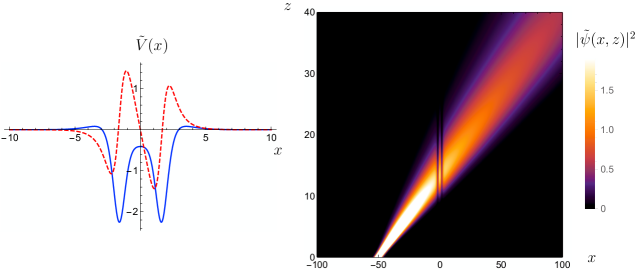
(a)

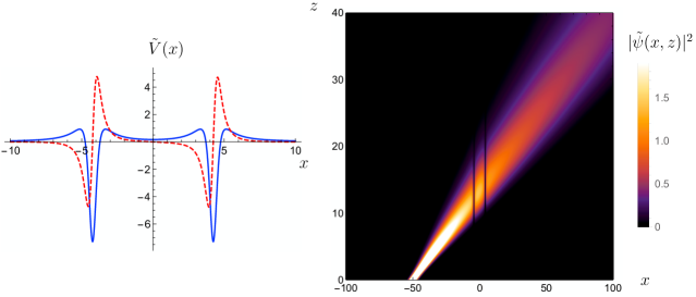
(b)

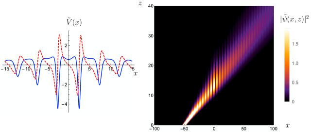
(c)

figure

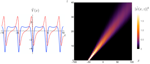
(d)

Figure 1: Reflectionless optical potentials. On the left: $PT$-symmetric potential $\tilde{V}(x)=-2\frac{d^{2}}{dx^{2}}\log\,\left(\int_{0}^{x}\psi_{0}^{2}(s)ds+i\alpha_{{}_{R}}\right)$ discussed in section 5.1. The solid blue (dashed red) line represents the real (imaginary) part. On the right: intensity $|\tilde{\psi}(x,z)|^{2}$ of the light beam when propagating through the optical potential. There is a bound state of energy with (a) $E_{0}=-k_{0}^{2}$, (b) $E_{0}=0$, (c) $E_{0}=k_{0}^{2}$. The periodic system (d) has no bound states. The respective $\psi_{0}$ and parameters for the construction of the potentials in each case are given as follows. (a) $\psi_{0}=\cosh(k_{0}x+i\tau)$, ${\alpha_{{}_{R}}}=1.15$, $k_{0}=0.7$, $\tau=1.4$ (b) $\psi_{0}=bx+ic$, ${\alpha_{{}_{R}}}=-2.8$, $b=-0.26$, $c=-0.5$ (c) $\psi_{0}=\cos(k_{0}x+i\tau)$, ${\alpha_{{}_{R}}}=4$, $k_{0}=0.7$, $\tau=1$ (d) $\psi_{0}=e^{ik_{0}x}$, ${\alpha_{{}_{R}}}=1$, $k_{0}=0.7$. In $\tilde{\psi}(x,z)$, we fix $\sigma=2$, $x_{0}=-50$ and $\omega_{0}=\pi/2$ in all the cases, see (5.17) and (5.18).

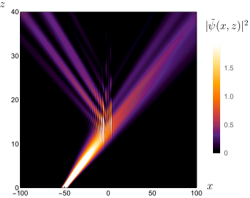
Figure 2: Reflective optical potential. Intensity $|\tilde{\psi}(x,z)|^{2}$ of the light beam when propagating through the real part of the potential, ${\rm Re}[\tilde{V}(x)]$, in the model (5.12). The parameters are the same as in (b) of Fig. 1. The two main reflections that appear about $x=0$ correspond to those produced by each potential well, see (b), Fig. 1.

5.2 One-gap systems

Let us take now the initial system described by the one-gap Lamé Hamiltonian,

$$H=-\frac{d^{2}}{dx^{2}}+V(x)\,,\qquad V(x)=2\kappa^{2}{\rm sn}^{2}\,(x,\kappa)-\kappa^{2}=-2\,{\rm dn}^{2}\,(x,\kappa)+1+\kappa^{\prime 2}\,.$$ (5.19)

The operator has period $2K$, where $K\equiv K(\kappa)$ is the complete elliptic integral of the first kind, $K(\kappa)=\int_{0}^{\pi/2}(1+\kappa^{2}\sin^{2}\phi)^{-1/2}d\phi$, $\kappa\in(0,1)$ is the modular parameter, and $\kappa^{\prime}=\sqrt{1-\kappa^{2}}$ is the complementary modular parameter . The spectrum of the Schrödinger operator $H$ consists of two bands. The finite (valence) band is formed by the energies $E\in[0,\kappa^{\prime}{}^{2}]$, and the infinite (conduction) band stretches over the interval $E\in[1,\infty)$. The functions

$$\Psi_{\pm}^{a}\left(x\right)=\frac{{\rm H}\left(x\pm a\right)}{\Theta\left(x\right)}\exp\left[\mp x{\rm Z}\left(a\right)\right]\,$$ (5.20)

solve the eigenstate problem

$$H\Psi_{\pm}^{a}\left(x\right)=E(a)\Psi_{\pm}^{a}\left(x\right),\quad E(a)={\rm dn}^{2}\,(a,\kappa)\,.$$ (5.21)

Here $\Theta$, ${\rm H}$, and ${\rm Z}$ are Jacobi’s Theta, Eta and Zeta functions, while parameter $a$ can take arbitrary complex values. The functions ${\rm dn}\,(x,\kappa)$, as well as ${\rm cn}\,(x,\kappa)$ and ${\rm sn}\,(x,\kappa)$ that will be used later on, are Jacobi elliptic functions.

The actual value of $a$ determines whether the function is bounded or unbounded. Let us write $a=\beta+i\gamma$, $\beta,\gamma\in\mathbb{R}$. The wave functions are unbounded (non-physical) when the corresponding energies belong to the lower infinite band, $E\in(-\infty,0)$, or to the finite spectral gap, $E\in(k^{\prime}{}^{2},1)$. This happens provided $\beta\in(0,K)$, and $\gamma=K^{\prime}$ or $\gamma=0$, respectively. The two bands of physical eigenvalues correspond to $\gamma=[0,K^{\prime}]$, and $\beta=K$ for a finite (valence), and $\beta=0$ for infinite (conduction) bands. The properties of the functions (5.20) with respect to the parity and complex conjugation were discussed in detail in [35], and their behavior under the composite $PT$ transformation is given by

$$PT\Psi_{\pm}^{iK+\beta}\left(x\right) = e^{i\frac{\beta\pi}{K}}\Psi_{\mp}^{iK+\beta}\left(x\right)\qquad\mbox{for}\quad\beta\in(0,K),$$ (5.22)

$$PT\Psi_{\pm}^{\beta}\left(x\right) = -\Psi_{\mp}^{\beta}\left(x\right)\qquad\mbox{for}\quad\beta\in(0,K),$$ (5.23)

$$PT\Psi_{\pm}^{K+i\gamma}\left(x\right) = \Psi_{\pm}^{K+i\gamma}\left(x\right)\qquad\mbox{for}\quad\gamma\in[0,K^{\prime}],$$ (5.24)

$$PT\Psi_{\pm}^{i\gamma}\left(x\right) = -\Psi_{\pm}^{i\gamma}\left(x\right)\qquad\mbox{for}\quad\gamma\in[0,K^{\prime}],$$ (5.25)

where (5.22) and (5.23) correspond to the lower semi-infinite forbidden band and the finite spectral gap, while Eqs. (5.24) and (5.25) correspond to the finite and infinite allowed bands, respectively.

As discussed in the preceding section, we can construct operators $\tilde{H}$ with bound states of arbitrary energy by taking $\psi_{0}$ as an appropriate linear combination of (5.20). In the current case, we deal with the situation where analytical calculation of $\tilde{V}$ and $\tilde{\psi}_{0}$ gets exceedingly difficult in general due to the term $\int_{0}^{x}\psi_{0}^{2}(s)ds$ whose analytical form is rather unreachable. We focus here to the special cases where $\psi_{0}$ is $2K$-periodic (${\rm dn}\,(x,\kappa)$), or $4K$-periodic (${\rm cn}\,(x,\kappa)$ and ${\rm sn}\,(x,\kappa)$), and corresponds to the band-edge energies. The band edge states and eigenvalues are given by the relations

$$H\,{\rm dn}\,(x,\kappa)=0,\quad H\,{\rm cn}\,(x,\kappa)=k^{\prime}{}^{2}\cdot{\rm cn}\,(x,\kappa)\,,\quad H\,{\rm sn}\,(x,\kappa)=1\cdot{\rm sn}\,(x,\kappa)\,.$$ (5.26)

Taking $\psi_{0}$ as one of the band-edge states, we get

$$\tilde{H}=H+\frac{4\kappa^{2}\,{\rm sn}\,(x,\kappa)\,{\rm cn}\,(x,\kappa)\,{\rm dn}\,(x,\kappa)}{S_{E}}+2\frac{F_{E}}{S_{E}^{2}}\,,$$ (5.27)

where we abbreviated

$$F_{E}=\left\{\begin{array}[]{r}\kappa^{4}\,{\rm sn}^{4}(x,\kappa)\,,\\ \kappa^{4}\,{\rm cn}^{4}(x,\kappa)\,,\\ \,{\rm dn}^{4}(x,\kappa)\,,\end{array}\right.\quad S_{E}=\left\{\begin{array}[]{rr}-x-i\kappa^{2}\tilde{\alpha}+{\rm E}(x,\kappa),&\psi_{0}=\,{\rm sn}\,(x,\kappa)\,,\\ -(1-\kappa^{2})x+i\kappa^{2}\tilde{\alpha}+{\rm E}(x,\kappa),&\psi_{0}=\,{\rm cn}\,(x,\kappa)\,,\\ i\tilde{\alpha}+{\rm E}(x,\kappa),&\psi_{0}=\,{\rm dn}\,(x,\kappa)\,.\end{array}\right.$$ (5.34)

Here, ${\rm E}(x,\kappa)$ is the incomplete elliptic integral of the second kind, ${\rm E}(x,\kappa)=\int_{0}^{x}{\rm dn}^{2}(s,\kappa)\,ds$. The extra potential terms (in addition to initial $V(x)$ from (5.19)) vanish for large $|x|$ (due to asymptotically linear behavior of $S_{E}$), so that $\tilde{V}$ coincides asymptotically with $V$. In [35], it was found that real periodicity defects, associated with discrete energies in the forbidden bands, induce phase shifts of the wave functions. In the current case, a $PT$-symmetric defect associated with the band-edge energy does not alter the asymptotic form of the wave functions.

Despite the explicit analytical form of $\tilde{H}$ for generic choice of $\psi_{0}$ is unreachable, we can still make some interesting conclusions. Let us discuss briefly the properties of the intermediate Hamiltonian $\breve{H}$ when $\psi_{0}=\Psi_{\pm}^{a}(x)$. As it was discussed in [35], in this case $\breve{H}$ coincides with the original but displaced Hamiltonian $H$,

$$\breve{H}(x)=H(x+a+iK^{\prime})-E_{0}\,,$$ (5.35)

where $K^{\prime}=K(\kappa^{\prime})$. Notice that $H(x+a+iK^{\prime})$ is $PT$ symmetric whenever $a=i\gamma$ or $a=K+i\gamma$ for $\gamma=[0,K^{\prime}]$, i.e. when $\Psi_{\pm}^{a}(x)$ corresponds to the physical state. We can fix the solutions of $(\breve{H}-E_{0})f=0$ in the following form,

$$\psi_{\pm}=\Psi_{\epsilon}^{a}(x+a+iK^{\prime})\pm PT\Psi_{\epsilon}^{a}(x+a+iK^{\prime}),\quad PT\psi_{\pm}=\pm\psi_{\pm},$$ (5.36)

where $\epsilon$ equals either $+$ or $-$. By the construction, (5.36) are eigenfunctions of $PT$. They are also quasi-periodic and bounded. In order to construct the Hamiltonian $\tilde{H}$, we fix $B$ in terms of $\eta_{0}$ which is a linear combination of $\psi_{+}$ and $\psi_{-}$. However, taking into account that

$$PT\Psi_{\pm}^{a}(x+a+iK^{\prime})=\left\{\begin{array}[]{l}-\Psi_{\pm}^{a}(x+a+iK^{\prime}),\quad a=i\gamma\,,\\ e^{\pm 2iK(\frac{\pi}{2K}-i\,{\rm Z}(a))}\Psi_{\pm}^{a}(x+a+iK^{\prime}),\quad a=K+i\gamma\,,\end{array}\right.$$ (5.39)

one can check that it is sufficient to consider only $\eta_{0}=\Psi_{\pm}^{a}(x+a+iK^{\prime})$. This gives

$$\tilde{H}=\breve{H}-2(\log\eta_{0})^{\prime\prime}=H(x+a+iK^{\prime})-2(\log\eta_{0})^{\prime\prime}=\left\{\begin{array}[]{l}H(x+2i\gamma),\quad\eta_{0}=\Psi_{+}^{a}(x+a+iK^{\prime})\,,\\ H(x),\quad\eta_{0}=\Psi_{-}^{a}(x+a+iK^{\prime})\,.\end{array}\right.$$ (5.42)

Clearly, $\tilde{H}$ has no bound state as $1/\eta_{0}$ is not quadratically integrable. Darboux transformation based on $\eta_{0}$ produces from $\breve{H}$ either the initial Hamiltonian $H(x)$ or its complex shifted copy $H(x+2i\gamma)$.

Finally, let us make a brief comment on the unbounded states (5.20) that can be written as $f_{\pm}=e^{k_{1}x}e^{ik_{2}x}u_{k_{0}}(x)$, $k_{1},k_{2}\in\mathbb{R}$. In the one-gap system, the value of $k_{2}$ distinguishes the valence and conduction bands; it is equal to $0$ for the states from the lower forbidden band, whereas $k_{2}=\frac{\pi}{2K}$ for the finite gap, see [35] for the details.

6 Hidden and exotic supersymmetric structures associated with finite-gap system $\tilde{H}$, and Jordan states

Spectrum of a generic periodic Hamiltonian possesses an infinite number of gaps and bands. However, there is a class of systems whose spectra contain just a finite number of gaps. If we denote the number of gaps as $n$, the free-particle Hamiltonian (5.1) represents the system with $n=0$, whereas the one-gap Lame Hamiltonian (5.19) qualifies for $n=1$. The peculiarity of having a finite number of gaps in the spectrum is associated with the existence of an integral of motion known as Lax-Novikov operator $\mathcal{L}$. This integral is represented by a $(2n+1)$-order differential operator.

In correspondence with the Burchnall-Chaundy theorem [78, 79, 80, 81], its square is a polynomial in $H$,

$$\mathcal{L}^{2}=\prod_{m=1}^{2n+1}(H-E_{m})\,,\qquad[H,\mathcal{L}]=0\,.$$ (6.1)

Here, $E_{m}$ are the energies corresponding to the edges of the allowed energy bands.

The Lax-Novikov integral reflects spectral degeneracy of the finite-gap system. It distinguishes two states corresponding to the doubly-degenerate energies in the interior of the bands. Particularly, in the one-gap case, the Bloch states (5.20) of the same energy are eigenstates of $\mathcal{L}$ of eigenvalues differing in sign. For the free particle (5.1), the Lax-Novikov integral coincides with the momentum operator $\mathcal{L}=-i\frac{d}{dx}$. It annihilates a constant, which is the wave function corresponding to zero energy. In the case of the one-gap Lamé system, the integral acquires a rather nontrivial form of the third order differential operator, that annihilates the band edge states ${\rm sn}(x,\kappa)$, ${\rm cn}(x,\kappa)$ and ${\rm dn}(x,\kappa)$, see [27, 28, 35] for its explicit form.

The operator $\tilde{H}$ constructed from a finite-gap Hamiltonian $H$ possesses the integral of motion obtained by a dressing procedure,

$$\tilde{\mathcal{L}}=BA\mathcal{L}A^{\sharp}B^{\sharp}\,,\qquad[\tilde{H},\tilde{\mathcal{L}}]=0\,.$$ (6.2)

When $\mathcal{L}$ is of order $2n+1$, then $\tilde{\mathcal{L}}$ has order $2n+5$. Making use of the intertwining relations, we find that $\tilde{\mathcal{L}}$ satisfies the relation

$$\tilde{\mathcal{L}}^{2}=(\tilde{H}-E_{0})^{4}\prod_{m=1}^{2n+1}(\tilde{H}-E_{m})\,.$$ (6.3)

The operator $\tilde{\mathcal{L}}$ inherits the properties of $\mathcal{L}$. Bloch solutions of the equation $(\tilde{H}-E)\tilde{\psi}=0$ corresponding to the double-degenerate energy level $E$ are also eigenstates of $\tilde{\mathcal{L}}$ of eigenvalues differing in sign. When $E$ corresponds to one of the non-degenerate band-edge energies $E_{m}$, $m=1,...,2n+1$, the corresponding physical states are annihilated by this operator. Let us clarify the point where $\mathcal{L}$ and $\tilde{\mathcal{L}}$ differ from each other. For the purpose we shall analyze the kernel of $\tilde{\mathcal{L}}$.

We suppose that $E_{m}\neq E_{0}$ for $m=1,...,2n+1$. There are $2n+1$ states $\tilde{\psi}_{m}$ in the kernel which are images of the states $\psi_{m}$ annihilated by $\mathcal{L}$,

$$\tilde{\psi}_{m}=BA\psi_{m}\,,\quad\mathcal{L}\psi_{m}=0\,,\quad m=1,...,2n+1\,.$$ (6.4)

Let us define auxiliary functions $\Sigma_{2}$ and $\Sigma_{3}$ that satisfy $\mathcal{L}\Sigma_{2}=\psi_{0}$ and $\mathcal{L}\Sigma_{3}=\chi.$ Then we find the remaining four vectors from the kernel of $\tilde{\mathcal{L}}$,

$$f_{0}=\eta_{0}^{-1}\,,\qquad f_{1}=\eta_{0}^{-1}\int_{0}^{x}\frac{\eta(s)}{\psi_{0}(s)}ds\,,$$ (6.5)

$$f_{2}=\eta_{0}^{-1}\int_{0}^{x}\frac{\eta_{0}(s)}{\psi_{0}(s)}\int_{0}^{s}\psi_{0}(r)\Sigma_{2}(r)drds\,,\qquad f_{3}=\eta_{0}^{-1}\int_{0}^{x}\frac{\eta_{0}(s)}{\psi_{0}(s)}\int_{0}^{s}\psi_{0}(r)\Sigma_{3}(r)drds\,.$$ (6.6)

Using the explicit form (2.3) and (2.24) of $A^{\sharp}$ and $B^{\sharp}$, one can check that there holds

$$B^{\sharp}f_{1}=-\psi_{0}^{-1}\,,\qquad A^{\sharp}B^{\sharp}f_{2}=\Sigma_{2}\,,\qquad A^{\sharp}B^{\sharp}f_{3}=\Sigma_{3}\,.$$ (6.7)

The functions $f_{1}$, $f_{2}$ and $f_{3}$ are the Jordan states of $\tilde{H}$ associated with $E_{0}$,

$$(\tilde{H}-E_{0})^{j}f_{j}=\frac{1}{\eta_{0}}\,,\quad(\tilde{H}-E_{0})^{j+1}f_{j}=0\,,\qquad j=1,2,3\,.$$ (6.8)

As it was shown in [27, 28], the finite-gap systems possess a hidden $N=2$ superalgebra graded by the parity operator $P$. The two supercharges, anticommuting with $P$, are given by $\mathcal{L}$ and $iP\mathcal{L}$. It was showed there that the superalgebraic structure is preserved by the Darboux-Crum transformation based on the band-edge states. In our current case, the intertwining operators $BA$ and $A^{\sharp}B^{\sharp}$ are $PT$-symmetric, however, they do not need to have a definite parity with respect to the space inversion $P$. Hence, as neither $\tilde{H}$ nor $\tilde{\mathcal{L}}$ have definite parity, $P$ is prevented from being a viable grading operator. Instead, we can consider the $PT$ symmetry operator, which commutes both with $H$ and $\mathcal{L}$. Let us define $\mathcal{L}_{1}=i\mathcal{L}$ and $\mathcal{L}_{2}=iPT\mathcal{L}$. These operators anticommute with $PT$, and generate the $N=2$ supersymmetry of $H$,

$$[\mathcal{L}_{a},H]=0\,,\quad\{\mathcal{L}_{a}\,,\mathcal{L}_{b}\}=-\delta_{ab}\prod_{n=1}^{2n+1}(H-E_{n})\,,\quad a,b=1,2\,.$$ (6.9)

Notice that the sign of the anticommutator is changed when compared to the Hermitian case discussed, for instance, in [27, 28]. As the intertwining operators $BA$ and $A^{\sharp}B^{\sharp}$ commute with $PT$, this superalgebraic structure can be identified easily in the system described by $\tilde{H}$ as well,

$$[\tilde{\mathcal{L}}_{a},\tilde{H}]=0\,,\quad\{\tilde{\mathcal{L}}_{a}\,,\tilde{\mathcal{L}}_{b}\}=-\delta_{ab}(H-E_{0})^{4}\prod_{m=1}^{2n+1}(H-E_{n})\,,\quad a,b=1,2\,,$$ (6.10)

where the supercharges are defined as $\tilde{\mathcal{L}}_{a}=BA\mathcal{L}_{a}A^{\sharp}B^{\sharp}$. The grading operator of the superalgera (6.10) is $PT$.

Let us make a brief comment on the finite-gap systems where the intermediate Hamiltonian satisfies $\breve{H}=H(x+c)$, see (5.8) or (5.35). In these cases, the Lax-Novikov operator associated with $\tilde{H}$ reduces to $(2n+3)$-order differential operator $\tilde{\mathcal{L}}(x)=B(x)\mathcal{L}(x+c)B^{\sharp}(x)$. It satisfies $\tilde{\mathcal{L}}^{2}=\prod_{m=1}^{2n+1}(\tilde{H}-E_{m})(\tilde{H}-E_{0})^{2}$.

The scheme given by the relations (6.9) and (6.10) corresponds to a bosonized supersymmetry, where no fermionic degrees of freedom are present in the system [82, 83, 84]. However, by using the confluent Darboux-Crum transformations, an extended, exotic supersymmetry can also be constructed. Let us define a matrix Hamiltonian,

$$\mathcal{H}=\left(\begin{array}[]{cc}H&0\\ 0&\tilde{H}\\ \end{array}\right),$$ (6.13)

which resembles the supersymmetric Hamiltonian of the standard supersymmetry, see [26]. Instead of having linear supercharges, we can construct a pair of supercharges of the second order based on the confluent Darboux-Crum transformations, by taking the Pauli matrix $\sigma_{3}$, $\sigma_{3}^{2}=1$, as the grading operator,

$$\mathcal{Q}_{1}=\left(\begin{array}[]{cc}0&A^{\sharp}B^{\sharp}\\ BA&0\\ \end{array}\right),\qquad\mathcal{Q}_{2}=i\sigma_{3}\mathcal{Q}_{1}\,.$$ (6.16)

The supercharges commute with the Hamiltonian and anticommute with $\sigma_{3}$, resulting in the following $N=2$ non-linear superalgebra,

$$\left[\mathcal{H},\mathcal{Q}_{a}\right]=0\,,\quad\{Q_{a},\sigma_{3}\}=0\,,\quad\{Q_{a},Q_{b}\}=2\delta_{ab}(\mathcal{H}-E_{0})^{2},\quad a,b=1,2\,.$$ (6.17)

The finite-gap nature of the Hamiltonians $H$ and $\tilde{H}$ guarantees the existence of integrals $\mathcal{L}$ and $\tilde{\mathcal{L}}$. They can be used to define two bosonic supercharges for $\mathcal{H}$,

$$\mathscr{L}_{1}=\left(\begin{array}[]{cc}(H-E_{0})^{2}\mathcal{L}&0\\ 0&\tilde{\mathcal{L}}\\ \end{array}\right),\quad\mathscr{L}_{2}=i\sigma_{3}\mathscr{L}_{1}\,.$$ (6.20)

In this definition, the polynomial $(H-E_{0})^{4}$ was inserted to keep the same differential order $2n+5$ of the diagonal elements (recall that $\mathcal{L}$ is of order $2n+1$ whereas $\tilde{\mathcal{L}}$ is of order $2n+5$). The bosonic and non-linear property of the integrals $\mathscr{L}$ are summarized in the following superalgebra,

$$\left[\mathcal{H},\mathscr{L}_{a}\right]=0\,,\quad[\mathscr{L}_{a},\sigma_{3}]=0\,,\quad\{\mathscr{L}_{a},\mathscr{L}_{b}\}=2\delta_{ab}(\mathcal{H}-E_{0})^{4}\prod_{m=1}^{2n+1}(\mathcal{H}-E_{m}),\quad a,b=1,2\,.$$ (6.21)

The full supersymmetric structure gets enlarged if we consider also a new set of fermionic integrals by multiplying the integrals (6.16) by the extended Lax-Novikov operator $\mathscr{L}_{1}$,

$$\mathcal{S}_{1}=\mathcal{Q}_{1}\mathscr{L}_{1}\,,\qquad\mathcal{S}_{2}=i\sigma_{3}\mathcal{Q}_{1}\mathscr{L}_{1}\,,$$ (6.22)

which satisfy

$$\left[\mathcal{H},\mathcal{S}_{a}\right]=0\,,\qquad\{S_{a},\sigma_{3}\}=0\,.$$ (6.23)

Finally, the nonlinear superalgebra can be completed by means of the remaining (anti)commutation relations,

$$[\mathcal{Q}_{a},\mathscr{L}_{2}] =-2\epsilon_{ab}\mathcal{S}_{b}\,,\qquad[\mathcal{S}_{a},\mathscr{L}_{2}]=-2\epsilon_{ab}\prod_{m=1}^{2n+1}(\mathcal{H}-E_{m})(\mathcal{H}-E_{0})^{4}\mathcal{Q}_{b}\,,$$ (6.24)

$$\{\mathcal{Q}_{a},\mathcal{S}_{b}\} =2\mathcal{S}_{a}\mathcal{Q}_{b}+2\delta_{ab}(\mathcal{H}-E_{0})^{2}\mathscr{L}_{1}\,.$$ (6.25)

Hence, the extended system (6.13) is characterized by exotic supersymmetric structure described by the four supercharges $\mathcal{Q}_{a}$ and $\mathcal{S}_{a}$, and the two bosonic integrals $\mathscr{L}_{a}$, which together generate the nonlinear superalgebra (6.17), (6.21), (6.23), (6.24), (6.25).

7 Discussion

We showed that the confluent Darboux-Crum (double-step Darboux-Jordan) transformation is an efficient tool for creating $PT$-symmetric systems that are asymptotically real and periodic, and have a periodicity defect disappearing for large $|x|$. We pointed out the difference between the confluent and usual second-order Darboux-Crum transformations. Whereas the intertwining operators of the standard one annihilate two (formal) eigenstates of the initial Hamiltonian, the intertwining operators of the generalized transformation annihilate, besides an eigenstate of $H$, also the associated Jordan state, see Eqs. (2.25), (2.24), (2.11) and (2.13).

The described confluent Darboux-Crum transformations were applied to a generic Hamiltonian with real even periodic potential (3.2). We discussed the general aspects of the construction like existence of (quadratically integrable) bound states and asymptotic behavior of the created systems. We showed that bound states in the continuous part of the spectrum are associated with invisibility of the periodicity defects.

It was also showed that the decay rate of the periodicity defect is determined by the position of the bound-state energy in the spectrum; when it belongs to the interior of the energy band or it can be identified with the band-edge energy, amplitudes of the defects disappear as $x^{-1}$ or $x^{-2}$. When the bound state corresponds to discrete energy in the energy gap or lower forbidden band, exponential decay of the defect takes place. It would be interesting to verify whether this observation is of general validity, i.e. whether a periodicity defect of the $1/x$ or $1/x^{2}$ decay induces a bound state in the energy continuum, whereas the defects with exponential decay are responsible for discrete energies.

The application of the generic results was focused on the special class of periodic systems that possess finite number of gaps in their spectra. In the subsection 5.1, we considered reflectionless systems derived by the confluent Darboux-Crum transformation from the free-particle model. In particular, we constructed reflectionless $PT$-symmetric systems which are completely invisible.

In the subsection 5.2, we discussed asymptotically periodic systems with periodicity defects derived from the one-gap system described by the Lamé equation. It is worth noticing that in the recent work [35], similar systems with soliton defects described by a Hermitian Hamiltonian were constructed from the one-gap Lamé system using standard Darboux-Crum transformations. There, an analysis was provided how to construct new Hamiltonians with periodicity defects, that induce bound states with discrete energy in the gap or in the lower forbidden band, below the valence band. The subsection 5.2 extends those results with the use of the generalized (confluent) Darboux-Crum transformations. It allowed us to construct systems with bound state energy of arbitrary value. In particular, we constructed explicit models where the bound state was associated with the band-edge energy. We also discussed the specific case where the intermediate Hamiltonian coincides with the original one up to a complex shift of coordinates.

In section 6, we discussed a set of integrals of motion associated with finite-gap systems, which give rise to bosonized and exotic supersymmetries. We showed in detail how the superalgebraic structure of the integrals of motion differs from the standard case when the supercharges based on the confluent Darboux-Crum transformation are taken into account.

Despite illustrating our results on the finite-gap systems, we would like to stress that the results of section 4 apply to a broad class of real even periodic potentials.

The invisibility of periodicity defects discussed in this paper resembles the Klein tunneling. This phenomenon occurs in relativistic quantum mechanics where spin-$1/2$ particles can tunnel through strong electrostatic barriers. When the particles are massless, the barrier becomes invisible for the particles in the sense that it has no effect on their dynamics, independently on its actual form. Although Klein tunneling was not observed for elementary particles, it is manifested in carbon nanostructures where dynamics is governed by one- or two-dimensional Dirac equation. There, it can cause absence of backscattering of Dirac fermions on impurities in carbon nanotubes, see e.g. [85] and references therein. In our case, the invisibility is very model-sensitive. On the contrary to the Klein effect, even a slight change of the potential can make it visible as the beam or particles start to scatter off it. The physics behind these two phenomena is distinct; whereas Klein tunneling stems on existence of solutions corresponding to antiparticles, invisibility discussed in this paper is rather the result of a fine interference of transmitted and reflected waves on the particular potential barriers.

Acknowldegments FC thanks M. Tudorovskaya for useful discussions and for her assistance and explanations about numerical methods. He is supported by the Alexander von Humboldt Foundation. VJ was supported by the GAČR Grant No.15-07674Y. FC and MP thank Nuclear Physics Institute of Czech Republic, where a part of this work was done, for hospitality. VJ is grateful for warm hospitality of the Universidad de Santiago de Chile. He is also grateful for warm hospitality that he experienced in CECs. CECs is funded by the Chilean Government through the Centers of Excellence Base Financing Program of CONICYT. We also acknowledge partial financial support from FONDECYT Grants No. 1130017 and 11121651, CONICYT Grant No. 79112034 (Chile), and Proyecto Basal USA 1298.

References

- [1] P. W. Milonni, in Coherence Phenomena in Atoms and Molecules in Laser Fields, edited by A. D. Bandrauk and S. C. Wallace (Plenum, New York, 1992), p. 45.
- [2] A. Guo, G. J. Salamo, D. Duchesne, R. Morandotti, M. Volatier-Ravat, V. Aimez, G. A. Siviloglou, and D. N. Christodoulides, Phys. Rev. Lett. 103, 093902 (2009).
- [3] C. E. Rüter, K. G. Makris, R. El-Ganainy, D. N. Christodoulides, M. Segev, and D. Kip, Nat. Phys 6, 192 (2010).
- [4] A. Regensburger, C. Bersch, M.-A. Miri, G. Onishchukov, D. N. Christodoulides, and U. Peschel, Nature 488, 167 (2012).
- [5] R. El-Ganainy, K. G. Makris, D. N. Christodoulides, and Z. H. Musslimani, Opt. Lett. 32, 2632 (2007).
- [6] K. G. Makris, R. El-Ganainy, D. N. Christodoulides, and Z. H. Musslimani, Phys. Rev. Lett. 100, 103904 (2008).
- [7] Z. H. Musslimani, K. G. Makris, R. El-Ganainy, and D. N. Christodoulides, Phys. Rev. Lett. 100, 030402 (2008).
- [8] K. G. Makris, R. El-Ganainy, D. N. Christodoulides, and Z. H. Musslimani, Phys. Rev. A 81, 063807 (2010).
- [9] M. C. Zheng, D. N. Christodoulides, R. Fleischmann, and T. Kottos, Phys. Rev. A 82, 010103 (2010).
- [10] M. V. Berry, J. Phys. A: Math. Gen. 31, 3493 (1998).
- [11] H. F. Jones, J. Phys. A 45, 135306 (2012) [arXiv:1111.2041 [physics.optics]].
- [12] A. Mostafazadeh, Phys. Rev. A 90, 023833 (2014) [arXiv:1407.1760 [quant-ph]]; Addendum: Phys. Rev. A 90, 055803 (2014).
- [13] Z. Lin, H.Ramezani, T. Eichelkraut, T. Kottos, H. Cao, and D. N. Christodoulides, Phys. Rev. Lett. 106, 213901 (2011) [arXiv:1108.2493 [physics.optics]].
- [14] A. Mostafazadeh, Phys. Rev. A 91, 063812 (2015) [arXiv:1504.01756]
- [15] S. Longhi, J. Phys. A: Math. Theor. 44, 485302 (2011) [arXiv:1111.3448 [quant-ph]].
- [16] A. Mostafazadeh, Phys. Rev. A 87, 012103 (2013) [arXiv:1206.0116 [math-ph]].
- [17] C. M. Bender, Rept. Prog. Phys. 70, 947 (2007) [hep-th/0703096 [HEP-TH]].
- [18] A. Mostafazadeh, Int. J. Geom. Meth. Mod. Phys. 7, 1191 (2010) [arXiv:0810.5643 [quant-ph]].
- [19] A. Mostafazadeh, Phys. Scripta 82, 038110 (2010) [arXiv:1008.4680 [quant-ph]].
- [20] A. Mostafazadeh, J. Phys. A 36, 7081 (2003), [arXiv:quant-ph/0304080];
- [21] C. M. Bender, J. Brod, A. Refig, and M. Reuter, J. Phys. A 37, 10139 (2004) [arXiv:quant-ph/0402026];
- [22] M. Znojil, Rendic. Circ. Mat. Palermo, Ser. II, Suppl. 72, 211 (2004) [arXiv:math-ph/0104012].
- [23] S. Klaiman, U. Gunther, and N. Moiseyev, Phys. Rev. Lett. 101, 080402 (2008), [arXiv:0802.2457 [quant-ph]].
- [24] E. M. Graefe and H. F. Jones, Phys. Rev. A 84, 013818 (2011) [arXiv:1104.2838 [physics.optics]].
- [25] C. M. Bender, D. C. Brody and H. F. Jones, Phys. Rev. Lett. 89, 270401 (2002) [Phys. Rev. Lett. 92, 119902 (2004)] [quant-ph/0208076].
- [26] F. Cooper, A. Khare, and U. Sukhatme, Phys. Rept. 251, 267 (1995), [arXiv:hep-th/9405029].
- [27] F. Correa, V. Jakubský, L. M. Nieto, and M. S. Plyushchay, Phys. Rev. Lett. 101, 030403 (2008) [arXiv:0801.1671 [hep-th]];
- [28] F. Correa, V. Jakubský, and M. S. Plyushchay, J. Phys. A 41, 485303 (2008) [arXiv:0806.1614 [hep-th]].
- [29] M. S. Plyushchay and L. M. Nieto, Phys. Rev. D 82, 065022 (2010), [arXiv:1007.1962 [hep-th]].
- [30] M. S. Plyushchay, A. Arancibia, and L. M. Nieto, Phys. Rev. D 83, 065025 (2011) [arXiv:1012.4529 [hep-th]].
- [31] A. Arancibia, J. M. Guilarte and M. S. Plyushchay, Phys. Rev. D 88, 085034 (2013) [arXiv:1309.1816 [hep-th]].
- [32] A. Arancibia and M. S. Plyushchay, Phys. Rev. D 90, no. 2, 025008 (2014), [arXiv:1401.6709 [hep-th]].
- [33] V. B. Matveev and M. A. Salle, Darboux Transformations and Solitons (Springer, Berlin, 1991).
- [34] F. Correa and M. S. Plyushchay, Annals Phys. 327, 1761 (2012) [arXiv:1201.2750 [hep-th]].
- [35] A. Arancibia, F. Correa, V. Jakubský, J. M. Guilarte, and M. S. Plyushchay, Phys. Rev. D 90, no. 12, 125041 (2014) [arXiv:1410.3565 [hep-th]].
- [36] S. M. Chumakov, K. B. Wolf, Phys. Lett. A 193, 51 (1994).
- [37] J. Radovanović, V. Milanović, Z. Ikonić, and D. Indjin, Phys. Rev. B 59, 5637 (1999).
- [38] J. Bai and D. S. Citrin, Optics Express 14, 4043 (2006).
- [39] M.-A. Miri, M. Heinrich, R. El-Ganainy, and D. N. Christodoulides, Phys. Rev. Lett. 110, 233902 (2013) [arXiv:1304.6646 [physics.optics]].
- [40] M. Heinrich, M.-Ali Miri, S. Stützer, R. El-Ganainy, S. Nolte, A. Szameit, and D. N. Christodoulides, Nat. Commun. 5, 4698 (2014) [arXiv:1401.5734 [physics.optics]].
- [41] M.-A. Miri, M. Heinrich, and D. N. Christodoulides, Optica 1, 89 (2014) [arXiv:1408.0832 [physics.optics]].
- [42] S. Longhi, Optics Letters 40, 463 (2015) [arXiv:1411.7144 [physics.optics]].
- [43] S. Longhi and G. Della Valle, Europhys. Lett. 102, 40008 (2013) [arXiv:1306.0677 [quant-ph]].
- [44] M. A. Miri, M. Heinrich, and D. N. Christodoulides, Phys. Rev. A 87, no. 4, 043819 (2013), [arXiv:1305.1689 [physics.optics]].
- [45] S. Longhi and G. Della Valle, Annals. Phys. 334, 35 (2013) [arXiv:1306.0667 [quant-ph]].
- [46] B. Midya, Phys. Rev. A 89, 032116 (2014) [ arXiv:1401.4996 [physics.optics]].
- [47] M. Principe, G. Castaldi, M. Consales, A. Cusano, and V. Galdi, Sci. Rep. 5, 8568 (2015).
- [48] S. Longhi, J. Opt. 17, 045803 (2015) [arXiv:1501.02063 [physics.optics]].
- [49] J. von Neumann and E. Wigner, Phys. Z. 30, 465 (1929).
- [50] J. Pappademos, U. Sukhatme, and A. Pagnamenta, Phys. Rev. A 48, 3525 (1993) [arXiv:hep-ph/9305336].
- [51] T. A. Weber and D. L. Pursey, Phys. Rev. A 50, 4478 (1994).
- [52] David J Fernández and Encarnación Salinas-Hernández, J. Phys. A: Math. Gen. 36, 2537 (2003)
- [53] D. J. Fernández C. and E. Salinas-Hernández, Phys. Lett. A 338, 13 (2005) [quant-ph/0502147].
- [54] C. D. J. Fernández and E. Salinas-Hernández, J. Phys. A 44, 365302 (2011) [arXiv:1105.2333 [quant-ph]].
- [55] A. Schulze-Halberg, Eur. Phys. J. Plus 128, 68 (2013)
- [56] A. Contreras-Astorga and A. Schulze-Halberg, Annals Phys. 354, 353 (2015).
- [57] H. C. Rosu, S. C. Mancas and P. Chen, Annals Phys. 343, 87 (2014).
- [58] H. C. Rosu, S. C. Mancas and P. Chen, Annals Phys. 349, 33 (2014) [arXiv:1311.6866 [math-ph]].
- [59] N. Prodanović, V Milanović, and J Radovanović, J. Phys. A: Math. Theor. 42, 415304 (2009).
- [60] J.S. Petrović, V. Milanović, and Z. Ikonić, Phys. Lett. A 300, 595 (2002).
- [61] D. C. Marinica, A. G. Borisov, and S. V. Shabanov Phys. Rev. Lett. 100, 183902 (2008).
- [62] E. N. Bulgakov and A. F. Sadreev, Phys. Rev. B 78, 075105 (2008).
- [63] S. Longhi, Opt. Lett. 39, 1697 (2014) [arXiv:1402.3761 [quant-ph]].
- [64] F. Cannata, G. Junker and J. Trost, Phys. Lett. A 246, 219 (1998), [arXiv:quant-ph/9805085].
- [65] C. M. Bender, G. V. Dunne and P. N. Meisinger, Phys. Lett. A 252, 272 (1999), [arXiv:cond-mat/9810369].
- [66] H.F Jones, Phys. Lett. A 262, 242 (1999).
- [67] J. M. Cerveró, Phys. Lett. A 317, 26 (2003).
- [68] K.C. Shin, J. Phys. A: Math. Gen. 37, 8287 (2004), [arXiv:math-ph/0404015].
- [69] B. F. Samsonov and P. Roy, J. Phys. A: Math. Gen. 38, L249 (2005), [arXiv:quant-ph/0503040].
- [70] W. Magnus and S. Winkler, Hill’s equation (Wiley, New York, 1966).
- [71] S. M. Klishevich and M. S. Plyushchay, Nucl. Phys. B 606, 583 (2001) [arXiv:hep-th/0012023].
- [72] M. Znojil, J. Phys. A 34, 9585 (2001) [arXiv:math-ph/0102034].
- [73] F. Correa and M. S. Plyushchay, Phys. Rev. D 86, 085028 (2012) [arXiv:1208.4448 [hep-th]].
- [74] P. Drazin and R. Johnson, Solitons: An Introduction (Cambridge University Press, Cambridge, England, 1996) (see Q1.12, p.18).
- [75] M. Znojil and M. Tater, J. Phys. A 34, 1793 (2001) [arXiv:quant-ph/0010087].
- [76] A. Fring, M. Znojil, J. Phys. A 41, 194010 (2008) [arXiv:0802.0624 [quant-ph]].
- [77] V. B. Matveev and M. A. Salle, Darboux Transformations and Solitons (Springer, Berlin, 1991).
- [78] J.L. Burchnall and T.W. Chaundy, Proc. London Math. Soc. Ser. 2, 21, 420 (1923).
- [79] J.L. Burchnall, T.W. Chaundy, Proc. Royal Soc. London A 118, 557 (1928).
- [80] E.L. Ince, Ordinary differential equations, (Dover, 1956).
- [81] I.M. Krichever, Funct. Anal. Appl. 12, 175 (1978).
- [82] M. S. Plyushchay, Annals Phys. 245, 339 (1996) [arXiv:hep-th/9601116].
- [83] M. S. Plyushchay, Int. J. Mod. Phys. A 15, 3679 (2000) [arXiv:hep-th/9903130].
- [84] V. Jakubský, L. M. Nieto and M. S. Plyushchay, Phys. Lett. B 692 (2010) 51 [arXiv:1004.5489 [hep-th]].
- [85] V. Jakubský, L. M. Nieto and M. S. Plyushchay, Phys. Rev. D 83, 047702 (2011) [arXiv:1010.0569 [cond-mat.mes-hall]].