Shape function in QED and bound muon decays

Abstract

When a particle decays in an external field, the energy spectrum of the products is smeared. We derive an analytical expression for the shape function accounting for the motion of the decaying particle and the final state interactions. We apply our result to calculate the muonium decay spectrum and comment on applications to the muon bound in an atom.

I Introduction

A bound particle decays differently than when it is free. Even in the ground state, due to the uncertainty principle, bound particles are in motion that causes a Doppler smearing of their decay products. In addition, if the charge responsible for the binding is conserved, daughter particles are subject to final state interactions.

Binding effects partially cancel in the total decay width Überall (1960); Czarnecki et al. (2000); Chay et al. (1990); Bigi et al. (1992). However, in some regions, the energy spectrum of the decay products can be significantly deformed. The range of the accessible energy can also be modified, by a participation of spectators.

In this paper we focus on weakly bound systems in quantum electrodynamics (QED) where the bulk of the decay products remains in the energy range accessible also in the free decay. The slight but interesting redistribution in that region is governed by the so-called shape function $S$ Neubert (1994a, b); Bigi et al. (1994); Mannel and Neubert (1994); De Fazio and Neubert (1999); Bosch et al. (2004). Here we present for the first time a simple analytical expression for $S$.

The shape function was first introduced to describe heavy quarks decaying while bound by quantum chromodynamics (QCD). It is employed in a factorization formalism based on the heavy-quark effective field theory (HQEFT) that separates the short-distance scale, related to the heavy-quark mass, from the long-distance nonperturbative effects governed by the scale $\Lambda_{\mathrm{QCD}}$, embodied in the shape function. In QCD it is a nonperturbative quantity that can be fitted using data but not yet derived theoretically.

The shape function formalism has been defined also for quarkonium Beneke et al. (1997). Subsequently in Beneke et al. (2000) a quarkonium production shape function was obtained analytically. Analytical results for the decay shape function in the ’t Hooft model were obtained in Grinstein (2006).

In QED, the shape function has recently been computed numerically and applied to describe the decay of a muon bound in an atom Czarnecki et al. (2014) (so-called decay in orbit, DIO). The spectrum of decay electrons consists of the low-energy part up to about half the muon mass $m_{\mu}$, and a (very suppressed) high-energy tail extending almost to the full $m_{\mu}$. The shape function formalism applies only to the former, also known as the Michel region Michel (1950).

In this paper we will not be concerned with the high-energy tail. We note here only that it is also of great current interest because it will soon be precisely measured by COMET Kuno (2013) and Mu2e Brown (2012). The high-energy part of the DIO spectrum is a potentially dangerous background for the exotic muon-electron conversion search, the main goal of these experiments. That region has therefore recently been theoretically scrutinized Czarnecki et al. (2011); Szafron and Czarnecki (2015).

II Factorization in Muonium

The HQEFT is based on the heavy quark mass being much larger than the nonperturbative scale $\Lambda_{\mathrm{QCD}}$. Similarly, in muonic bound states there exists a hierarchy of scales Szafron (2013): the mass of the decaying muon is much larger than the typical residual momentum, $m_{\mu}\gg p$. In a muonic atom we have

$$p\sim m_{\mu}Z\alpha,$$ (1)

while in muonium

$$p\sim m_{e}\alpha,$$ (2)

where $\alpha\approx{1}/{137}$ is the fine structure constant and $m_{e}$ is the electron mass.

With this observation, the factorization formula and the shape function for the muon DIO were derived in Czarnecki et al. (2014) using earlier QCD results Neubert (1994a, b); Mannel and Neubert (1994); De Fazio and Neubert (1999); Bosch et al. (2004). Here we follow an equivalent but a slightly more general approach Bigi et al. (1994) to derive the differential rate for a heavy charged particle decay in the presence of an external Coulomb field, neglecting radiative effects. We apply the result to find the decay spectrum of muonium.

We concentrate on the muon decay $\mu^{+}\rightarrow e^{+}\bar{\nu}_{\mu}\nu_{e}$ but our results are general and apply to any QED bound state decay, provided that the momentum in the bound state is much smaller than the decaying particle mass.

The decay amplitude is related to the imaginary part of the two-loop diagram depicted in Fig. 1.

Figure 1: Muon self-energy diagram whose imaginary part corresponds to the muon decay rate. Double line for charged particles indicates the electromagnetic interaction with the spectator electron that needs to be resummed.

Integrating over the relative neutrino momentum we express the differential decay rate as

$$\mathrm{d}\Gamma=2G_{F}^{2}\mathrm{Im}\left(h_{\alpha\beta}\right)W^{\alpha\beta}\frac{\mathrm{d}^{4}q}{(2\pi)^{3}},$$ (3)

where $q$ is the sum of neutrino four-momenta and $G_{F}$ is the Fermi constant Webber et al. (2011); Marciano (1999). The neutrino tensor is

$$W^{\mu\nu}=-\frac{\pi}{3(2\pi)^{3}}q^{2}\left(g^{\mu\nu}-\frac{q^{\mu}q^{\nu}}{q^{2}}\right).$$ (4)

The charged-particle tensor $h_{\mu\nu}$ can be decomposed using five scalar functions that depend on $q^{2}$ and $v\cdot q=q_{0}$. Here $v$ is the four-velocity of the bound state. In general,

$$h_{\mu\nu}=-h_{1}g_{\mu\nu}+h_{2}v_{\mu}v_{\nu}-ih_{3}\epsilon_{\mu\nu\rho\sigma}v^{\rho}q^{\sigma}$$

$$+h_{4}q^{\mu}q^{\nu}+h_{5}\left(q_{\nu}v_{\mu}+q_{\mu}v_{\nu}\right),$$ (5)

but since the neutrino tensor (4) is symmetric under $\mu\leftrightarrow\nu$, from now on we neglect the asymmetric part of $h$. Contracting the tensors and denoting $w_{i}=\mathrm{Im}(h_{i})$ we find that only two functions $w_{1,2}$ suffice to describe the double differential spectrum,

$$\frac{\mathrm{d}\Gamma}{\mathrm{d}q^{2}\mathrm{d}q_{0}}=\frac{G_{F}^{2}}{3\left(2\pi\right)^{4}}\left[3q^{2}w_{1}-\left(q^{2}-q_{0}^{2}\right)w_{2}\frac{}{}\right]\sqrt{q_{0}^{2}-q^{2}}.$$ (6)

Functions $w_{i}$ can be calculated in QED. Adopting Schwinger’s operator representation Schwinger (1989), we have instead of the free electron propagator

$$\frac{1}{\not{k}-m_{e}}\rightarrow\frac{1}{\not{k}+\not{\pi}-m_{e}},$$ (7)

where $\pi^{\mu}$ is defined such that it does not contain any heavy degrees of freedom. The commutator of its components gives the electromagnetic field-strength tensor $[\pi^{\mu},\pi^{\nu}]=-ieF^{\mu\nu}$ where $e$ is the muon charge. Formally,

$$h_{\mu\nu}=2\left\langle M\left|\overline{\mu}\gamma_{\mu}\frac{1}{\not{k}+\not{\pi}-m_{e}}\gamma_{\nu}\left(1-\gamma_{5}\right)\mu\right|M\right\rangle,$$ (8)

where $|M\rangle$ denotes the bound-muon state and $k=m_{\mu}v-q$. Equation (8) is valid in the whole phase space.

To simplify our considerations, we restrict ourselves to the Michel region where the electron is almost on-shell, $k^{2}\sim m_{\mu}\,p$ and the time component of $k$ is large, $v\cdot k\gg p$. This is the region where binding effects are most prominent. (Near the highest energies also the virtuality is much higher, $k^{2}\sim m_{\mu}^{2}$, permitting a perturbative expansion of the electron propagator Szafron and Czarnecki (2015).) We neglect the electron mass since the electron is highly relativistic Mannel and Neubert (1994); Shifman (1995). The only effect of the electron mass is an overall shift of the endpoint spectrum, just like in a free-muon decay.

In the Michel region, the four-momentum $k$ can be written as $k=(v\cdot k)n+\delta k$, where $n$ is a lightlike vector, $n^{2}=0$, and $\delta k\sim p$. Neglecting terms suppressed by $\frac{p^{2}}{m^{2}_{\mu}}$,

$$h_{\mu\nu}=4\left(2m_{\mu}v_{\mu}v_{\nu}-\nu\cdot kg_{\mu\nu}-v_{\nu}q_{\mu}-v_{\mu}q_{\nu}\right)$$

$$\times\left\langle M\left|\frac{1}{k^{2}+2\left(\pi\cdot n\right)\left(k\cdot v\right)}\right|M\right\rangle.$$ (9)

We cannot further expand the denominator since both terms are of order $m_{\mu}\,p$. We introduce $\lambda=-\frac{k^{2}}{2k\cdot v}$; it will be useful to remember that $\lambda$ scales like the muon momentum $\lambda\sim p\sim Z\alpha$. We now define the shape function,

$$S(\lambda)=\left\langle M|\delta(\lambda-n\cdot\pi)|M\right\rangle,$$ (10)

and obtain

$$w_{1} = 2\pi S(\lambda),$$ (11)

$$w_{2} = \frac{4m_{\mu}}{k\cdot v}\pi S(\lambda)=\frac{2m_{\mu}}{k\cdot v}w_{1}.$$ (12)

We have recovered the QCD scaling behavior Bjorken (1969): functions $w_{i}$ depend in the leading order only on the ratio of $k^{2}$ and $v\cdot k$ rather than on these two variables separately.

Equation (10) reveals that the shape function is closely related to the momentum distribution of the muon in the bound state. However, due to gauge invariance we cannot replace $n\cdot\pi$ by the momentum in the $\vec{n}$ direction.

III Shape function

Formula (10) is the same for muonium and for a muonic atom. Both systems are nonrelativistic, therefore the wave function needed to calculate the expectation value in (10) has the same analytical form. The only difference is its parameters and thus the physical scales that characterize the muon momentum $p$ [see below, Eq. (15)]. We now proceed to an explicit calculation of the function $S$ in Eq. (10).

The bound-state wave function follows from field theory via the Bethe-Salpeter equation Salpeter and Bethe (1951). In the non-relativistic limit it reduces to the Schrödinger equation,

$$\left(\frac{\vec{p}^{\,2}}{2\mu}+V(r)\right)\psi_{S}(r)=E\psi_{S}(r),$$ (13)

where $\mu$ is the reduced mass of the system. In the case of a muonic atom, with the mass of the nucleus $m_{N}$,

$$\mu=\frac{m_{\mu}m_{N}}{m_{\mu}+m_{N}}\approx m_{\mu}.$$ (14)

Subsequent formulas apply to muonium with the following substitutions,

$$m_{\mu} \rightarrow m_{e},$$

$$m_{N} \rightarrow m_{\mu},$$

$$Z \rightarrow 1.$$ (15)

For example, the reduced mass in muonium is

$$\mu=\frac{m_{e}m_{\mu}}{m_{e}+m_{\mu}}\approx m_{e}.$$ (16)

With this notation we also have $p\sim Z\alpha\mu$.

As customary, Eq. (13) is written in the Coulomb gauge, with the electromagnetic four-potential given by

$$eA_{\mu}(x)=\left(V(r),0,0,0\right),$$ (17)

with $V(r)=-\frac{Z\alpha}{r}$ for a muonic atom or $V(r)=-\frac{\alpha}{r}$ for muonium. The determination of the shape function is especially convenient in the so-called light-cone gauge,

$$n^{\mu}A_{\mu}(x)=0.$$ (18)

In this gauge, the electron is effectively free up to effects quadratic in the electromagnetic field. The price for this simplification is a more complicated formula for the muon wave function. In the light-cone gauge, Eq. (10) takes a simple form in the momentum representation,

$$S(\lambda)=\int\frac{{\mathrm{d}}^{3}k}{(2\pi)^{3}}\psi_{S}^{\star}\left(\vec{k}\right)\delta\left(\lambda+\vec{n}\cdot\vec{k}\right)\psi_{S}\left(\vec{k}\right).$$ (19)

We are neglecting terms of order $(Z\alpha)^{2}$ in the above expression. To fulfill condition (18), we change the gauge,

$$eA_{\mu}^{\prime}(x)=eA_{\mu}(x)+\partial_{\mu}\chi(x),$$ (20)

with

$$\chi(x)=\chi(\vec{x})=Z\alpha\ln\left(\vec{n}\cdot\vec{r}+r\right).$$ (21)

This transformation changes the muon Schrödinger wave function in the 1S state, $\psi_{S}(r)$, by an $\vec{r}$-dependent phase factor, such that

$$\psi_{S}(r)\rightarrow\psi(\vec{r})=e^{-i\chi(\vec{r})}\psi_{S}(r)=\left(\vec{n}\cdot\vec{r}+r\right)^{-iZ\alpha}\psi_{S}(r).$$ (22)

After the transformation, the wave function is no longer rotationally invariant, since the gauge fixing distinguishes the direction of the outgoing electron.

We use the Schwinger parametrization,

$$\frac{\Gamma(\alpha)}{A^{\alpha}}=\int_{0}^{\infty}dtt^{\alpha-1}\exp\left[-At\right]$$ (23)

to Fourier-transform Eq. (22),

$$\psi(\vec{k}) = \int d^{3}r\exp\left(-i\vec{k}\cdot\vec{r}\right)\psi(\vec{r})$$ (24)

$$= \frac{iZ\alpha}{\Gamma(iZ\alpha)\sin\left(i\pi Z\alpha\right)}\frac{8\sqrt{\mu^{3}Z^{3}\alpha^{3}\pi^{3}}}{\left(\mu^{2}Z^{2}\alpha^{2}+\vec{k}^{2}\right)^{2}}\left(\frac{\mu^{2}Z^{2}\alpha^{2}+\vec{k}^{2}}{2\left(\mu Z\alpha-i\vec{n}\cdot\vec{k}\right)}\right)^{iZ\alpha}\left[\frac{\mu^{2}Z^{2}\alpha^{2}+\vec{k}^{2}}{2\left(\mu Z\alpha-i\vec{n}\cdot\vec{k}\right)}-\mu(i+Z\alpha)\right].$$

We integrate in (19) first over $\vec{n}\cdot\vec{k}$ using the delta-function, then over $\vec{k}_{\perp}$, components of $\vec{k}$ perpendicular to $\vec{n}$,

$$S(\lambda)=\frac{2\mu^{3}Z^{6}\alpha^{6}}{3\sinh(\pi Z\alpha)}\frac{3\lambda^{2}+6\lambda\mu+\mu^{2}\left(4+Z^{2}\alpha^{2}\right)}{\left[\lambda^{2}+\mu^{2}Z^{2}\alpha^{2}\right]^{3}}e^{2Z\alpha\arctan\left(\frac{\lambda}{\mu Z\alpha}\right)}.$$ (25)

The exponential function in (25) arises from $\left|\left(\mu Z\alpha+i\lambda\right)^{-iZ\alpha}\right|^{2}$, appearing after integrating $|\psi(\vec{k})|^{2}$ with the delta-function in (19). The leading behavior can be understood with the help of integral

$$\int d^{2}k_{\perp}\frac{1}{\left(\vec{k}^{2}_{\perp}+\lambda^{2}+\mu^{2}Z^{2}\alpha^{2}\right)^{4}}\sim\frac{1}{(\lambda^{2}+\mu^{2}Z^{2}\alpha^{2})^{3}}.$$ (26)

The result (25) contains subleading terms, related to the Coulomb potential in (10), required by the gauge invariance. At the current stage of calculations $S(\lambda)$ is explicitly gauge independent. We can drop subleading terms to obtain a leading-order formula,

$$S(\lambda)=\frac{8\mu^{5}Z^{5}\alpha^{5}}{3\pi\left[\lambda^{2}+\mu^{2}Z^{2}\alpha^{2}\right]^{3}}.$$ (27)

The analytical formula obtained here is useful for several reasons. First of all, counting powers and remembering that $\lambda\sim p$, we find that $S(\lambda)\sim\frac{1}{p}\sim\frac{1}{Z\alpha}$. This reminds us that $S(\lambda)$ is a nonperturbative object and explains why its effect on the spectrum can be quite dramatic, as we shall see in muonium in Sec. IV.

Further, Eq. (25) allows us to better control the expansion and the resummation of the $p$ effects in the decay spectrum. This cannot be done so easily with a numerical evaluation Czarnecki et al. (2014), as is especially clear when we analyze the first three moments, useful in HQEFT for constraining possible forms of the shape function.

The zeroth order moment gives just the normalization. With the normalized wave function in Eq. (19), the shape functions (25) and (27) are automatically normalized to unity; this is a consequence of the definition (10).

When the subleading terms are neglected the first moment of the shape function (27) vanishes,

$$\int\mathrm{d}\lambda\lambda S(\lambda)=\langle n\cdot\pi\rangle=0+\mathcal{O}(Z^{2}\alpha^{2}).$$ (28)

Naive power counting in the left-hand side suggests a result linear in $Z\alpha$. That leading part vanishes, similarly to the first moment of the B-meson shape function. A contribution linear in $\frac{p}{m_{\mu}}\sim Z\alpha$ is absent due to the CGG/BUV theorem Chay et al. (1990); Bigi et al. (1992). Moments of the shape function are related to matrix elements of local operators in the heavy particle effective theory. Operators of dimensions 3 and 5 exist. A dimension 4 operator that could generate, in the leading order, a nonvanishing first moment is missing. A nonzero first moment can only appear at the subleading order Neubert (1994b, a).

The second moment is related to the square of the average momentum in the direction of $\vec{n}$,

$$\int\mathrm{d}\lambda\lambda^{2}S(\lambda)=\frac{1}{3}\left\langle\vec{p}^{\,2}\right\rangle+\mathcal{O}\left(Z^{4}\alpha^{4}\right).$$ (29)

In contrast to the first moment, there is no cancellation here and the naive counting correctly predicts a result quadratic in $Z\alpha$. Therefore we do not need subleading corrections in Eq. (II) to calculate (29). This moment characterizes the width $\sigma_{\lambda}$ of the region smeared due to the shape function effects. As expected, it is of the same order as $p$: $\sigma_{\lambda}=\frac{Z\alpha\mu}{\sqrt{3}}$. This is similar to the HQEFT where the second moment is also related to the average kinetic energy of the heavy quark inside a meson.

In muonic aluminum, the stopping target of the planned conversion searches (Mu2e and COMET), the shape function effect is sizeable since $\sigma_{\lambda}\sim 6\,\text{MeV}$, and has been precisely measured by TWIST Grossheim et al. (2009). In the case of the muonium the effect is much smaller, $\sigma_{\lambda}\sim 2\,\text{keV}$, and is negligible except near the end of the spectrum.

In Fig. 2 we plot the shape function for $Z\alpha=0.25$. The width is proportional to $p$, suggesting that the dominant effect is due to the muon motion in the initial state.

Figure 2: Leading shape (27) function for $\mu=1$ MeV and $Z\alpha=0.25$. The width is $\sigma_{\lambda}=\mu\frac{Z\alpha}{\sqrt{3}}$. To illustrate it better we included two vertical dashed lines at the ends of $\sigma_{\lambda}$ region.

Finally, we would like to point out that the formula (27) can guide phenomenological models of the shape function in QCD. Some QCD bound states can be described with the help of effective theories similar to nonrelativistic QED Caswell and Lepage (1986); Lepage and Thacker (1988). For example, Ref. Jin and Paschos (1998) postulated a similar functional form of the shape function,

$$S(\lambda)=N\frac{\lambda(1-\lambda)}{(\lambda-b)^{2}+a^{2}}\theta(\lambda)\theta(1-\lambda),$$ (30)

with parameters $a,b$ to be fitted from data. Our function has a higher power of the denominator, therefore does not require an artificial restriction of its support by $\theta$ functions, because its tails are sufficiently suppressed.

IV Muonium spectrum

Having obtained the shape function, we can calculate the muonium spectrum using (6). After an integration over $q^{2}$, the electron energy is given by $E_{e}=m_{\mu}-q_{0}+\mathcal{O}(Z^{2}\alpha^{2})$. The shape function formalism can be interpreted as a replacement of the zero-width on-shell relation for the electron by a finite-width shape function $S(\lambda)$. (If $S(\lambda)$ in the functions $w_{i}$ is replaced by the Dirac-delta on-shell condition, the free-muon decay spectrum results.) Since the muon is almost at rest, the smearing is negligible far from the free muon decay endpoint, the only region where the spectrum is quickly varying with the electron energy.

We ignore the tail of the spectrum at energies higher than the free endpoint plus several $\alpha m_{e}$. It is very suppressed and its evaluation requires perturbative corrections due to hard photons Szafron (2013); Szafron and Czarnecki (2015). We also ignore the lowest region of the spectrum where positronium can be formed Greub et al. (1995).

For illustration, Fig. 3 shows the muonium decay spectrum in the vicinity of the free muon endpoint. The extent of the region affected by the shape function corresponds to the smearing width $\sigma_{\lambda}$, denoted by two vertical lines. In this region the slope of the spectrum is proportional to the shape function $S(\lambda)$ and therefore is of the order of $\frac{1}{p}\sim\frac{1}{\sigma_{\lambda}}$.

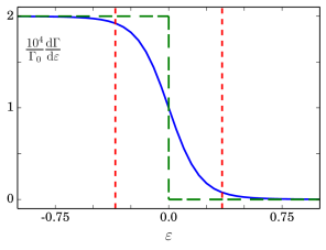
Figure 3: Endpoint region of the muonium decay. Electron energy is parametrized in terms of $\varepsilon$, such that $\varepsilon=10^{4}\frac{E_{e}-E_{\text{max}}}{E_{\text{max}}}$, $E_{\text{max}}=\frac{m_{\mu}^{2}+m_{e}^{2}}{2m_{\mu}}$. Dashed (solid) line shows the free-muon (muonium) spectrum. Vertical dotted lines emphasize the size of the region that is smeared due to binding effects.

Note that the free-muon decay, denoted with the dashed line, resembles a step function. This is an artefact of the very narrow width of the region shown in this figure. In fact, the free-decay spectrum varies with $\varepsilon$ to the left of the step and vanishes to the right of it.

V Conclusions

We have derived an analytical formula for the shape function and used it to calculate the muonium decay spectrum. Shape function moments were analyzed and compared with appropriate expressions in HQEFT. Our analytical formula may also have a limited application to describe nonrelativistic QCD systems. For now, the analytical expression for the shape function has improved our understanding of the approximations used in the derivation of the muon DIO spectrum.