Star Streams in Triaxial Isochrone Potentials with Sub-Halos

Abstract

The velocity, position, and action variable evolution of a tidal stream drawn out of a star cluster in a triaxial isochrone potential containing a sub-halo population reproduces many of the orbital effects of more general cosmological halos but allows easy calculation of orbital actions. We employ a spherical shell code which we show accurately reproduces the results of a tree gravity code for a collisionless star cluster. Streams from clusters on high eccentricity orbits, $e\gtrsim 0.6$, can spread out so much that the amount of material at high enough surface density to stand out on the sky may be only a few percent of the stream’s total mass. Low eccentricity streams remain more spatially coherent, but sub-halos both broaden the stream and displace the centerline with details depending on the orbits allowed within the potential. Overall, the majority of stream particles have changes in their total actions of only 1-2%, leaving the mean stream relatively undisturbed. A halo with 1% of the mass in sub-halos typically spreads the velocity distribution about a factor of two wider than would be expected for a smooth halo. Strong density variations, “gaps”, along with mean velocity offsets, are clearly detected in low eccentricity streams for even a 0.2% sub-halo mass fraction. Around one hundred velocity measurements per kiloparsec of stream will enable tests for the presence of a local sub-halo density as small as 0.2-0.5% of the local mass density, with about 1% predicted for 30 kiloparsec orbital radii streams.

1. INTRODUCTION

Tidal star streams pulled out from star clusters have been extensively studied in simulations where the galaxy is modeled as an analytic potential, often taken to be spherically or axially symmetric for simplicity (McGlynn, 1990; Johnston et al., 1996; Dehnen et al., 2004; Küpper et al., 2008; Varghese et al., 2011; Küpper et al., 2012; Amorisco, 2014; Fardal et al., 2014; Ngan & Carlberg, 2014; Carlberg, 2015; Hozumi & Burkert, 2015). These simulations have described how tidal heating ejects stars into a stream. There is a good analytic understanding of how sub-halos interact with thin streams in angular momentum conserving potentials to create velocity perturbations which open up to gaps in a stream (Yoon, Johnston & Hogg, 2011; Carlberg, 2012; Erkal & Belokurov, 2015). Simulations that begin with a cosmological halo show considerably more orbit diffusion than smooth analytic potentials (Bonaca et al., 2014; Pearson et al., 2015; Ngan et al., 2015a, b) which is not yet well understood. However, the increased orbital freedom is certainly related to the rich orbit structure in static triaxial potentials (de Zeeuw, 1985; Binney & Tremaine, 2008) which is bound to play a role in the aspherical and non-stationary cosmological galactic halos in which tidal streams develop.

In principle, kinematic measurements along a stream can tightly constrain the full phase space parameters of the highly redundant orbits of the stream particles and can serve as a precision probe of a galactic potential (Johnston et al., 1999; Binney, 2008; Bovy, 2014). The initial velocities of streams of stars that are tidally stripped from star clusters are calculated for a given orbit and potential with collisionless n-body codes. The stars emerge with highly correlated orbital velocity substructure (Carlberg, 2015). The stream width scales with the tidal radius and the length of scales with the tidal radius and the age of the stream (Johnston, 1998). In a spherical potential angular momentum and radial action are always conserved, but tidal mass loss features blur out with orbital overlap down the stream. However as stars move away from the progenitor on slightly different orbits in which the gravitational field has variations due to aspherical structure in the halo the streams can disperse relative to to a simple smooth potential model (Bonaca et al., 2014; Ngan et al., 2015b). Relative to a spherical potential the streams are almost everywhere increased in width, with some portions greatly blurred. However, a few segments of high or even enhanced density can remain (Ngan et al., 2015b). The view of the stream in the dynamical action variables, which are adiabatically conserved quantities of a potential, can provide insight into what is causing the stream to change its appearance (Ibata et al., 2002).

The purpose of this paper is to quantitatively analyze the dynamical behavior of tidal streams in moderately aspherical potentials that also contain a sub-halo population. The analysis will be done within a simplified potential which is able to reproduce many of the features of a cosmological halo but allows the calculation of action-angle variables at the beginning and end of the simulation. A simplified n-body code that reproduces the tidal stream from a standard n-body code is used to speed up the simulations. The changes in angular momentum and the radial action along a stream as a function of the halo shape and sub-halo content appear as changes to the stream in position and velocity space. These results will be useful to advance the understanding of the mass structure and contents of galactic halos as more and better kinematic data become available and serve as a guide to more realistic simulations.

2. Orbits in Triaxial Isochrone Potentials

We want to analyze the orbit changes of a stellar stream in a galactic halo with sub-halos. Action variables, as conserved quantities, provide direct insight into what has changed. Henon’s isochrone potential has simple algebraic expression for the actions (Henon, 1959a, b) and provides a reasonable match to a galactic rotation curve over the range of radii where we want to study stream dynamics. One fairly standard way to create a triaxial potential is to apply a linear scaling to the Cartesian coordinates of a spherical potential to create a triaxial potential. The simplicity of the axis scaling comes at the cost of losing the analytic properties of the orbits in the spherical potential. A number of axisymmetric potentials with good analytic properties have been developed (Eyre & Binney, 2011; Binney, 2014) but these still do not have the triaxiality, or more generally, the asphericity, of cosmological halos.

With the goal of allowing the rich orbital structure of a triaxial potential yet retaining some of the analytic properties of the isochrone, we introduce a time dependent potential, which for cosmological halos should be a reasonable approximation. The potential starts as a spherical isochrone, makes a smooth transition to a triaxial form, then remains as a triaxial for a relatively long interval, then reverses to become spherical again. The scale radius and the mass remain constant, the shape being only thing that changes. We will leave the $x$ axis unaltered, but compress the $y-z$ axes, which alters the density profile, increasing the density in the central region and generally leading to negative densities at large radius on the most compressed axis. We will also smoothly turn on and off a small fraction of the mass in an identically distributed sub-halo population.

The potential’s spherical initial and final form is a device to allow the analytic actions to be calculated and is not intended to be realistic. The action variables of the spherical isochrone will be valid quantities to calculate at the beginning and end of the simulation, although they are not conserved quantities over the simulation. We expect that there will be smooth changes in the action variables associated with the turn-on and turn-off of the triaxiality, and local changes as a result of sub-halo encounters, the two being sufficiently different that it might be possible to untangle the effects. Based on these considerations the triaxial isochrone potential used here is,

$$\Phi(x,y,z,t)={-GM(t)\over{b+\sqrt{b^{2}+x^{2}+y^{2}q_{y}^{-2}(t)+z^{2}q_{z}^{-2}(t)}}}.$$ (1)

The $q_{y}(t)$ and $q_{z}(t)$ are dimensionless functions which begin and end at unity, at which time the potential is spherically symmetric. We largely focus on compressions where the $q$ values are less than one, but cosmological halos also undergo small expansions during mergers with other halos as they. Our standard compression has $q_{y}=0.9$ and $q_{z}=0.95$ which leads to small negative densities on the $y$ axis beyond $y=6.51$, with a negative peak at $y=8.83$ with about $10^{-4}$ of the central density. The negative densities occur outside of the orbits that will be studied. The gravitational force is always inward directed.

2.1. Time Variation of Potential Shape

The potential asphericity turn-on takes place over a time $t_{r}$, after which it remains on for a time $t_{f}$, using the arbritrary function,

$$A(t)= 2(t/t_{r})^{2} 0\leq t\leq t_{r}/2,$$

$$= 1-2(1-t/t_{r})^{2} t_{r}/2<t\leq t_{r},$$

$$= 1 t_{r}<t<t_{f}+t_{r}.$$ (2)

For $t>t_{f}+t_{r}$ the rising function is reversed and $A(t)$ returns smoothly back to zero. The rise time, $t_{r}$, is chosen to reasonably slow, typically about 3 radial orbits, which is neither in the impulsive regime nor truly in the adiabatic regime. The time spent as a constant triaxial potential, $t_{f}$, is typically about 15 radial orbits, comparable to the time over which thin streams have been developing in the Milky Way halo.

All calculations here use units with $GM=1$ and $b=1$. We usually start the calculation with a cluster placed at an $x$ position of 4 units. We characterize the starting conditions with the angular momentum, $L$, relative to the angular momentum of a circular orbit in the spherical potential, $L_{c}$. Orbits with $L/L_{c}$ of 0.4 and 0.7 have radial orbital periods are 29.2 and 35.3, respectively, in the spherical potential when started at $r=4$. For the time variation function $A(t)$ we select $t_{r}=80$ and $t_{f}=440$, so that the potential becomes spherical again at time 600 and the simulation terminates.

The co-ordinate distortions are evaluated as $q_{y}(t)=1+a_{y}A(t)$ and $q_{z}(t)=1+a_{z}A(t)$. Positive $a_{y},a_{z}$ correspond to an expansion of the potential, that is, reduced gravitational attraction at locations off the $x$ axis and negative values correspond to a compression. Both expansion and compression are possible in cosmological situations, although compression likely dominates and is relatively small, since accreted mass spends little time in the central region and largely deposits mass near the current virial radius of the halo. Cosmological halos also can have a rotation of the potential shape, which we will ignore at this time. Louis & Gerhard (1988) studied radial perturbations to the isochrone potential finding that higher order resonances quickly appeared along with complex orbits, leading us to expect behavior of that sort.

2.2. Orbiting Sub-Halos

Sub-halos are present in large numbers in the dark matter halos created in cosmological simulations (Klypin et al., 1999; Moore et al., 1999; Diemand, Kuhlen & Madau, 2007; Springel et al., 2008; Stadel et al., 2009). The differential mass distribution is $m\,dN/dm\propto m^{-0.9}$ hence has nearly a constant mass per decade of mass, $m^{2}\,dN/dm\propto m^{0.1}$. The mass fraction of sub-halos varies steeply with radius relative to the local dark matter density in cosmological halos (Springel et al., 2008). For the radial range around 30 kpc where the few known thin streams have been found the models predict about 1% of the mass is in sub-halos, with the sub-halo mass fraction dropping to about 0.1% at a nominal solar radius of 8 kpc.

For the interests of this paper the practical issue is to have a well defined sub-halo population over the radial range of the star cluster orbit. Conceptually our approach is to convert a small fraction, $f_{sh}$, of the mass of the fixed isochrone potential into a set of sub-halos with the same collective massive distribution as the isochrone. The sub-halos are free to orbit within the isochrone potential as test particles, which requires that they be randomly drawn from a distribution function which generates the isochrone potential. Conveniently analytic forms are available for the isochrone’s mass and energy distribution functions (Hénon, 1960; Binney, 2014). Therefore on the average there is no change in the summed sub-halo plus diminished external potential, and, on the average, the global and local sub-halo fractions are equal everywhere for the initial spherical potential. Although the density distribution of the isochrone extends to infinity, 59% of the mass is within the $r=4$ orbit where we start the star clusters. Hence, little computational effort is wasted on the relatively few sub-clusters at larger radii which do not have orbital pericenters within the range of radii that the star cluster explores. The sub-halos respond to the undiminished triaxial isochrone potential but not each other. The stars of the cluster and the tidal streams feel gravitational forces from all other stars, plus the isochrone reduced by $(1-f_{sh}A(t))$ plus the sum of the forces from all the sub-halos which vary as $f_{sh}A(t)$. where the $A(t)$ factor, Equation 2, which rises from zero and returns to zero at the end of the simulation.

All the sub-halos are given identical masses, thereby allowing us to examine mass dependent effects. That is, once a number, $N_{sh}$, of sub-halos is chosen, the sub-halo all have mass, $m_{sh}=f_{sh}/N_{sh}$. Each sub-halo is modeled as a Herquist potential,$-Gm/(r+a)$, (Hernquist, 1990), with a scale radius $a_{sh}=\sqrt[3]{m_{sh}}$, as expected for cosmological sub-halos of constant scale density. The dependence of the results on the scale radius of the sub-halos are visible in the simplified analytic analysis (Carlberg, 2015; Erkal & Belokurov, 2015), where there is little change beyond the scale radius, but the induced velocities increase for stars that have encounters that take them within the scale radius of a sub-halo.

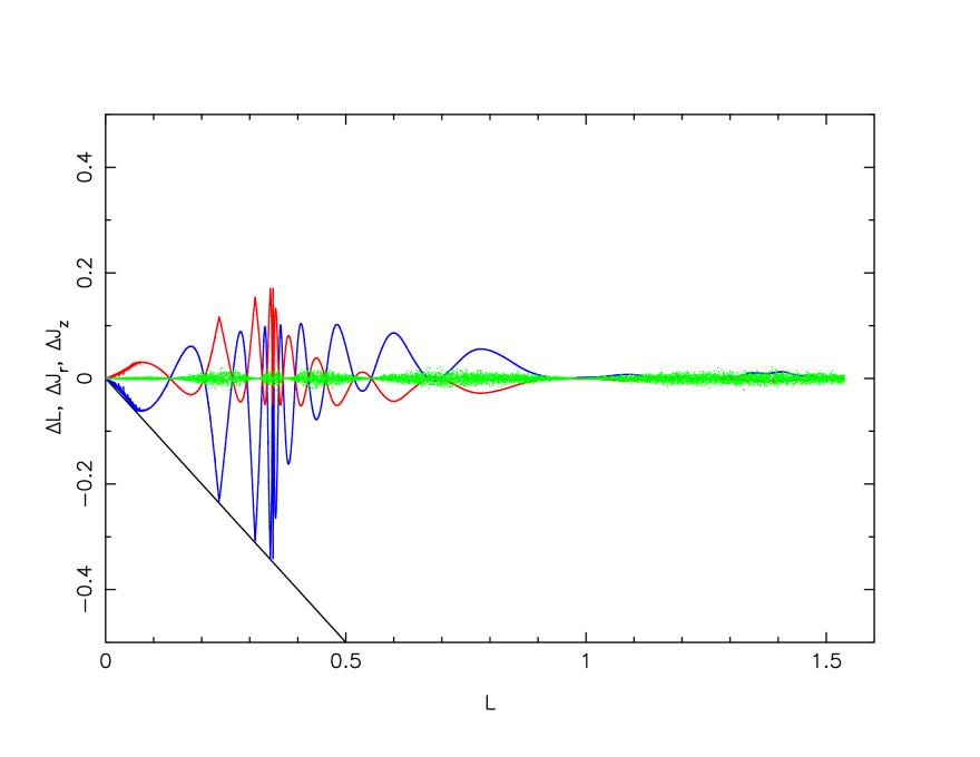
Figure 1.— The changes between beginning and end of the simulation in the particle’s total angular momentum, $L$ (blue), radial action $J_{r}$ (red) and angular momentum about the axis perpendicular to the initial orbital plane, $J_{z}$ (green), as a function of the initial $L$ in a potential with $a_{y}=-0.05$ and $a_{z}=-0.10$. The particles are started at $r=4$ with a uniform angular momentum distribution between 0 and the circular value. All orbits are started in the plane with an initial vertical and radial velocity dispersion of 0.002 units. A point below the downward sloping line drawn from the origin would have had its orbital direction reversed.

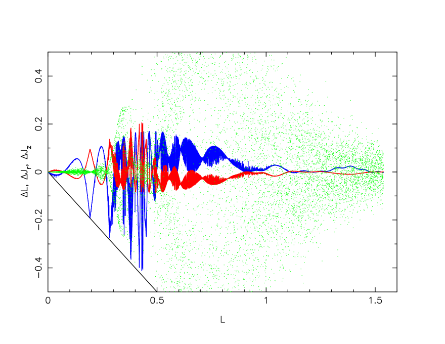
Figure 2.— Same as Fig. 1 but for $a_{y}=-0.10$ and $a_{z}=-0.05$.

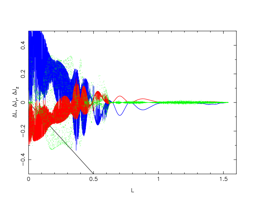
Figure 3.— Same as Fig. 1 but for $a_{y}=0.05$ and $a_{z}=0.10$.

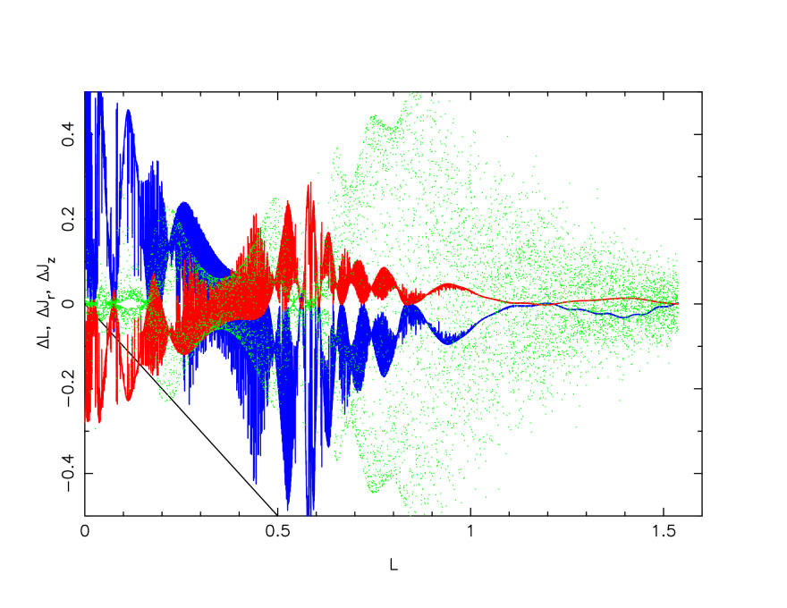
Figure 4.— Same as Fig. 1 but for $a_{y}=0.10$ and $a_{z}=0.05$.

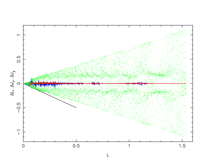
Figure 5.— Same as Fig. 2, with an increased vertical axis, but for $t_{r}=2400$, which is 30 times slower than the standard rate of potential change. The green dots are the changes in $J_{z}$.

2.3. Test Particle Orbits Without Sub-halos

Simple orbit integrations in the model potentials illustrate some of the potential’s basic properties. We start a set of 10,000 particles with no self-gravity at $x=4$, $y=z=0$ with a uniform distribution in $v_{y}$ between zero and the circular value at the chosen starting radius. The value of $x=4$ is chosen to help avoid the core region where there is little effective tidal force. The particle $v_{x}$ and $v_{z}$ velocities are given a small Gaussian random value, 0.002 units, about 0.5% of the circular velocity, to allow the particles to explore mildly off plane orbits. The orbits are integrated with a leapfrog integrator with step sizes of 0.004 units, which is nearly $10^{4}$ steps per orbit, conserving the actions to better than one part in $10^{6}$.

Orbits are evolved in four different versions of the triaxial isochrone, with $a_{y},a_{z}$ values of $\pm 0.05$ and $\pm 0.1$. The differences of the actions of the particles calculated at the start and end of the orbit integrations are plotted as a function of the initial orbital angular momentum in Figures 1, 2, 3 and 4. Figure 1 shows changes roughly as one might expect as a function of the orbital angular momentum (green points). That is, the range of initial orbital angular momentum means that particles have different orbital phasing relative to the changing axes. Some particles experience a net positive torque and others where the torques lead to a net loss. At high $L$, hence low eccentricity, the torques largely cancel out, leaving little net change.

In contrast to the simple behavior of Figure 1, Figures 2, 3 and 4 show nearly chaotic behavior over a range of orbits (Siegal-Gaskins & Valluri, 2008). The change in potential axis length remains the same as in Figure 1, but with the $yz$ axes switched, Fig. 2, or, made positive, hence allowed to expand, Figs. 3 and 4. The figures show that nearby orbits have dramatic differences in the changes to their action variables for higher eccentricity orbits. Low eccentricity orbits at high angular momentum are generally much less affected, although the vertical action can still be dramatically affected. This behavior is often seen for orbits that have higher order resonances between orbits and the rate of potential shape change.

If the potential changes are made very slowly we expect that the action changes for regular orbits will become adiabatic and become exponentially small (Binney & Tremaine, 2008). In Figure 5, the $\Delta L$ and $\Delta J_{r}$ actions diminish as expected but the changes in the $\Delta J_{z}$ values remain large. Overall, the rich range of orbital behavior of the triaxial isochrone makes it a simplified, but interesting, stand-in for a cosmological galactic halo potential that can capture realistic star stream behavior beyond a spherical halo.

2.4. Test Particle Orbits With Sub-halos

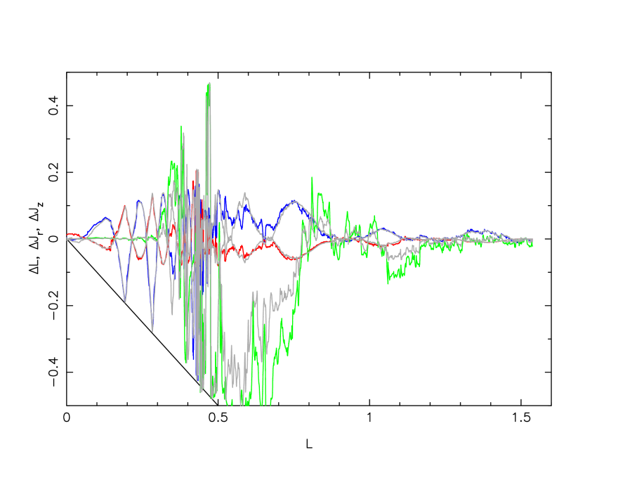
Figure 6.— Orbit integrations for the potential of Fig. 2 with 1000 sub-halos that total to 1% of the halo mass. The grey lines show the same simulation with the sub-halos reduced in mass by two. Here the particles are initiated with no additional random velocities. The inset shows the same simulation with no sub-halos.

The effects of adding sub-halos to the simple orbit integrations of Figure 2, are shown in Figure 6, where 1% of the halo mass transfers to 1000 identical mass sub-halos. That is, each sub-halo has a mass $10^{-5}$ of the host halo. The test particles are initiated with no additional random velocities to avoid the confusion of orbit diffusion. The outcome with no sub-halos is shown as the inset in Figure 6.

The sub-halo interactions occur on the scale of the radius of the sub-halos, which is approximately 0.02 units for the case studied. The sub-halos act to create fairly abrupt changes in the action variables, spread out over the orbits in accord with the density profile of the halo. Reducing the mass of each sub-halo by a factor of two, which reduces their scale radius by $\sqrt[3]{2}$, we find that the sharp changes in $J_{z}$ for $L\gtrsim 0.8$ are one half the height of the higher mass sub-halo results, indicating that single sub-halo encounters dominate for test particle orbits in this range over the duration of the simulation. For $L\lesssim 0.8$ the particles encounter sub-halos multiple times leading to much larger $J_{z}$ changes. The highest eccentricity orbits, those with $L\lesssim 0.3$ are largely unperturbed by sub-halos, likely because of their high velocities through the central regions. Overall the amplitude of the changes in the actions due to sub-halos are comparable to the changes due to the triaxial potential. We can foresee that disentangling sub-halo effects from potential effects will not be straightforward as might be hoped.

3. Simulation of a Small Star Cluster

Figure 7.— The mass in the cluster as a function of time on an $L/L_{c}=0.4$ orbit evolved with an $m=10^{-7}$ with a full n-body code (solid line) and with a shell code (dashed line).

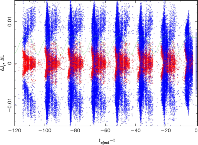
Figure 8.— The angular momentum (blue) and radial action (red) relative to the cluster center, $\Delta L,\Delta J_{r}$, respectively of particles as a function of their ejection time for the cluster evolved in the Gadget2 n-body code.

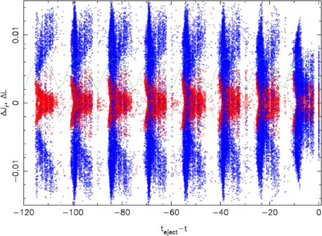
Figure 9.— The same model as Fig. 8 but evolved with the shell code.

We create a small, self-gravitating satellite of mass of $m\ll 1$ ($m\sim 10^{-8}$, where the host halo has $M_{I}=1$) from a King model distribution function (King, 1966). The cluster is created with its own dimensionless units of velocity and position, then scaled down in size to fit its zero density radius within the estimated tidal radius. The velocities are scaled to the desired mass and new size. Our standard star cluster model has a central potential, $\psi(0)$, relative to the central velocity dispersion, $\sigma$, of $-\psi(0)/\sigma^{2}=4$. Increasing $-\psi(0)/\sigma^{2}$ decreases the core radius relative to the radius where the model density goes to zero. The outer density profile has a slope nearly independent of the core radius, so the mass loss into the tidal stream has a weak dependence on the concentration of the model star cluster. Consequently the star cluster’s core radius only begins to have a significant effect on the tidal stream when mass loss is so large that the core is eroded.

The outer radius of the star cluster model is scaled to be equal to the tidal radius, $r[m/(3M_{I}(r))]^{1/3}$, where $r$ is the starting radius of the orbit. The small adjustment to the tidal radius for a distributed mass potential (Binney & Tremaine, 2008) is not included, nor is any allowance for a non-circular orbit, which leads to some modest internal changes of the star cluster model in response to the tidal field in its first orbit.

The standard model uses $10^{5}$ particles in the initial star cluster. The star particles in the model star clusters are subject to gravitational forces from other star particles, the host galaxy gravitational potential, and any orbiting sub-halos that may be present. The rate of mass ejection varies around the orbit and leads to complex, strongly correlated, velocity differences (or action variable offsets) between the stream and the star cluster (Carlberg, 2015). The mass loss in the systems of interest is driven by tidal heating and is well modeled with a collisionless n-body code. As a reference, we use the gravitational and orbital evolution components of the well known and characterized Gadget2 code (Springel, 2005).

3.1. An n-body shell code

The precise description of the evolution of a star cluster in the tidal field of a host galaxy remains an important research problem as a generalization of the dynamics of an isolated star cluster. Current work allows for a realistic range of star masses, their mass evolution and their remnants, the presence of binaries and higher multiplicity systems. The evolution of collisional star clusters in tidal fields generally either use some form of gravitational calculation splitting to handle the dynamics on different time scales (Fujii et al., 2007) or interactions via statistical approximations (Sollima & Mastrobuono Battisti, 2014; Brockamp et al., 2014). Fukushige & Heggie (2000) demonstrate the complexity of star cluster orbits near the tidal radius that exists for cluster in a circular orbit.

Two well known thin star streams are Pal 5, which emanates from an exceptionally low concentration cluster (Odenkirchen et al., 2001) and GD-1, which has no known progenitor (Grillmair & Dionatos, 2006). Given the complexity and high computational costs of studying a collisional star cluster, and, the observational fact that the importance of star-star encounters in the progenitor clusters is either relatively low, or, unknown, it is currently conventional to study tidal streams as emanating from tidally heated collisionless star clusters (Dehnen et al., 2004). Given that our interest is in the subsequent dynamics of the star streams the assumption is appropriate for the time being, but it will eventually be important to incorporate a more complete dynamical description of the originating star cluster.

The evolution of a very low mass, collisionless, satellite orbiting in an external potential in which dynamical friction is not a factor is well handled with multipole expansion codes. The relatively low cost and good accuracy of multipole n-body codes has a rich history as the first codes that could handle large numbers of self-gravitating collisionless particles (Aarseth, 1967; van Albada & van Gorkom, 1977; Fry & Peebles, 1980; Villumsen, 1982; White, 1983; McGlynn, 1984). Multipole methods remain popular for moderately distorted spheres with arbitrary density profiles for which there are now efficient parallel processing algorithms (Meiron et al., 2014) and have been generalized to the powerful self-consistent field method (Hernquist & Ostriker, 1992). A multipole field provides substantial smoothing of the gravitational field and completely suppresses the complex astrophysics of the two and more body interactions in a dense globular cluster. If desired, star-star collisional physics can be added using a Monte Carlo method (Giersz, 2006) although none is included here.

After testing potentials calculated with up to fourth order multipole expansions we found that a simple shell code, which only calculates the spherical part of the gravitational field, gave results that were essentially indistinguishable, with the shell code being less subject to the problem of defining the center. This is not unexpected in the situation we are modeling since much of the mass of the satellite is in the central regions where the tidal field is weak. On the other hand, the degree of quantitative accuracy needs to be verified. The shell code calculates the radial gravitational acceleration of a particle at radius, $r$ with a mildly softened gravity, $-GM(<r)r/(r^{2}+s^{2})^{3/2}$ where $M(<r)$ is simply the total mass interior to $r$ relative to a central point. The softening $s$ is set at 20% of the core radius of the King model cluster we wish to simulate and is needed for the case where two particles are near the coordinate center. Making a good choice for the central point of the potential is important, since a poor choice can lead to undesirable oscillations and even an unstable cluster. For the situations of interest here the simple approach of integrating the orbit of a fictitious particle placed at the position of the coordinate center of the cluster works extremely well and shows no signs of instability.

The calculation sorts particles in order of ascending radii and then calculates the gravitational field at each successive particle, simply as the mass interior to its radius. The sub-halo gravity is calculated with a direct sum. Our shell code has fixed time steps, $\Delta t=0.004$, that accurately capture the tidal heating in the star cluster and the interactions with sub-halos down the tidal stream. For many of our simulations about half of the particles remain in the cluster so increasing the time step size for particles outside the cluster would not necessarily give rise to a large speed increase. The code was parallelized with a parallel quicksort and MPI routines to reduce the execution time. Other than the quicksort the algorithm is essentially trivially parallel.

3.2. Comparison of n-body and shell code results

As tests of the accuracy of the shell code, Figure 7 shows the mass as a function of time in Gadget2 and the shell code for a cluster started at $r=2.2$ in a spherical isochrone. Note that difference between the full n-body code and the shell code is almost entirely one of slightly different orbital periods, not of mass lost per orbit. The shell code uses the high accuracy orbit of the center of the star cluster. The angular momentum and the radial action calculated at the end of the simulation when the potential is again spherical are measured relative to the star cluster as a function of their time of ejection from the cluster. The resulting distributions are shown for the n-body simulation in Figure 8 and for the shell code in Figure 9. The two are essentially identical, other than the slight difference in the orbital period, with the shell code having the correct period. We conclude that the shell code gives accurate results for the range of satellites, orbits and potentials of interest here.

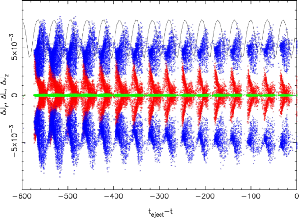
Figure 10.— The changes of the actions of particles of a stream from a cluster started with $L/L_{c}=0.7$ in a smooth triaxial with $[a_{y},a_{z}]=[-0.1,-0.05]$ (top) and $[-0.05,-0.1]$ (bottom) The actions are measured at the end of the simulation in the spherical potential relative to the cluster center values. The differences are plotted as a function of the time since the particle was ejected from the cluster. The action variables are red for $\Delta J_{r}$, blue for angular momentum, $\Delta L$ and green for $\Delta J_{z}$ whose values are scaled downward by a factor of 30 in this plot.

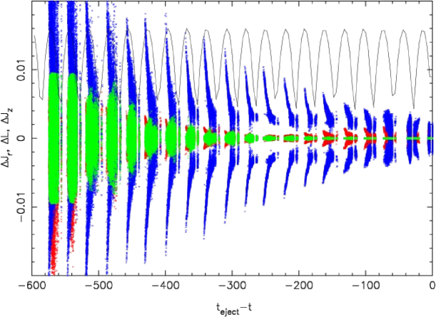
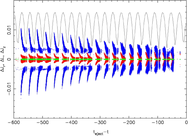
Figure 11.— Same as Figure 10 but with a cluster started with $L/L_{c}=0.4$. Note that the vertical scale is reduced relative to Fig. 10.

3.3. Streams in Triaxial Potentials without Sub-Halos

Clusters were started at $x=4$ with $L/L_{c}=0.7$ and $0.4$ in spherical and $[a_{y},a_{z}]=[-0.1,-0.05]$ triaxial isochrones with no sub-halos. A cluster in a low eccentricity orbit initiated with $L/L_{c}=0.7$ loses 39% of their mass over the interval to time 600 nearly independent of triaxiality. The cluster undertakes approximately 17 radial orbits in the spherical potential. Over the same time a cluster on a high eccentricity orbit loses 99.7% of its mass in the the triaxial potential and 94% in the spherical potential (21 radial orbits). Although the difference is easily measurable, when considered as a rate the differences with potential shape are small compared to the dependence on orbital eccentricity. The mass loss does depend on the location of the surface used to measure contained mass. We use 0.03 units, approximately three times the initial tidal radius.

Figures 10 and 11 show the action variables relative to the star cluster of the particles in the stream as function of their ejection age for two triaxial potentials. Two clear features are that the two tidal tails remain almost completely symmetric, largely a consequence of the small size of the cluster, which has a tidal radius of 0.007 units, about 0.3% of the orbital radius. Consequently, the tidal field is essentially symmetric across the cluster and the two tails are nearly the same, although moving away from the cluster in opposite directions. The second feature is that the radial action and angular momentum of the stars relative to the satellite vary slowly and smoothly over the duration which particles in the stream. The change of the angular momentum in the initial orbital plane, $\Delta J_{z}$, is largely a measure of the subsequent tilt of the orbits. $\Delta J_{z}$ rises exponentially with time, the doubling time being approximately 4 radial orbits. The exponential growth of the orbit tipping is an important new feature that the triaxial potential brings into play for the tidal stream relative to an orbit started with the same velocities in a spherical or axisymmetric potential. As the lower panels of Figures 10 and 11 show the same triaxility on different axes relative to the orbital plane does not show the exponential growth. Hence, orbital structure will depend on the details of the potential and the initial orbits of particles in the potential.

4. Streams in Triaxial Potentials with Sub-Halos

Two star clusters started with the same velocites in the $a_{y}=-0.1$, $a_{z}=-0.05$ halo of Figures 11 and 10, but now with 1000 sub-halos containing 0.5% of the mass of the halo, is shown in projection (both at two times) onto the orbital plane in Figure 12. The addition of the sub-halos leads to gaps in the stream and helps to push the progenitor and stream onto a somewhat different orbits relative to the same potential without sub-halos.

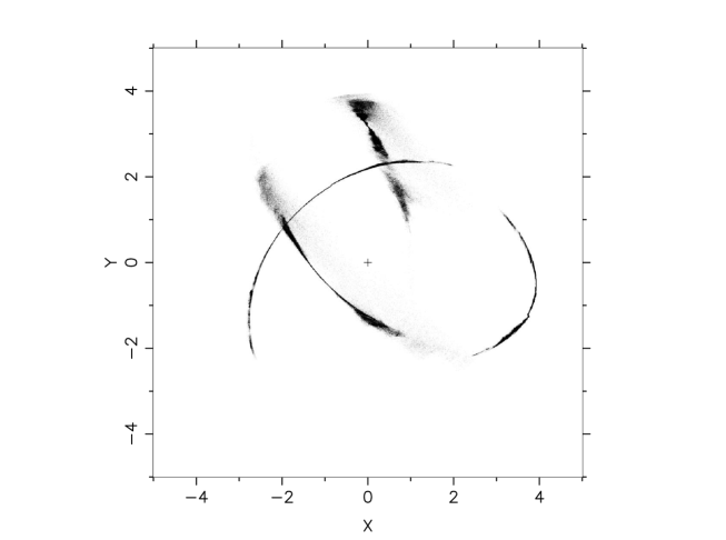
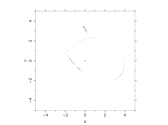
Figure 12.— Snapshots at times 580 and 600 of a low and high eccentricity stream. In the top panel the low eccentricity stream is the two blurry structures that come near the center, whereas the high eccentricity stream is the thinner structures that cross them and nearly connect. The contrast scale goes from 0 to 10 particles per 0.01 unit square pixel in the top panel and from 20 to 100 particles per pixel in the bottom.

4.1. Stream Visibilities

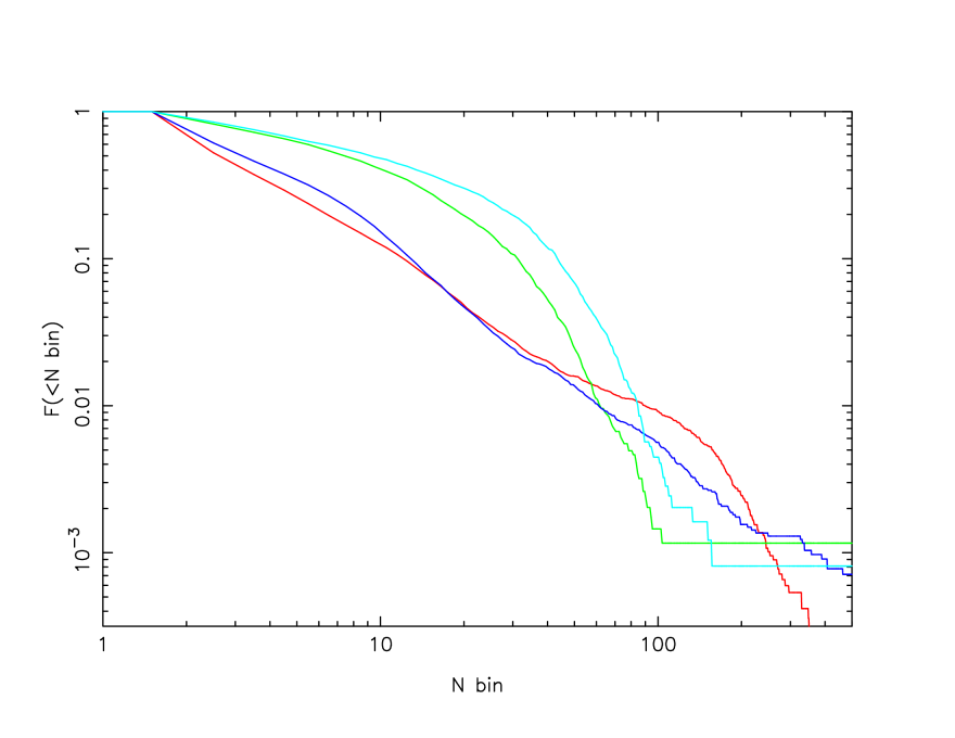
Figure 13.— The cumulative distribution, normalized to the total, of surface densities in the low eccentricity stream (green and turquoise lines) and the high eccentricity stream at times 580 and 600 (red and blue lines) in the $[-0.1,-0.05]$ halo shown in Fig 12.

A star cluster on a high eccentricity orbit is subject to stronger tidal fields at pericenter than a low eccentricity cluster with the same apocenter. The high eccentricity orbit also takes the stream into regions where there are more sub-halos, therefore we expect high eccentricity streams to have more orbital spreading than low eccentricity streams. To examine this idea we compare the streams from clusters on $L/L_{c}=0.4$ and 0.7 orbits in Figure 12. A cluster started with $L/L_{c}=0.4$ loses mass at more than twice the rate of a cluster started with $L/L_{c}=0.7$. Over the somewhat arbitrary simulation duration here the high eccentricity mass cluster is reduced to a few percent of its initial mass and it is only a coincidence of timing that the final moment is caught. Figure 12 shows the projected view of the two streams at two snapshot times. The upper panel shows the location of all particles, showing that the high eccentricity stream has many stars scattered well away from the stream. In currently available observational data, once match filtered to identify streams, it usually is difficult to identify stream locations where the local surface density is less than about a factor of 5 in density below the peak values (Carlberg & Grillmair, 2013).

Figure 13 shows that the surface density distribution of high and low eccentricity streams have a different character, with low eccentricity streams having relatively more paricles at higher surface densities. The distribution is not strongly orbital phase dependent. The peak values are similar, with about 100 particles per pixel (each pixel is 0.01 units square) for both low and high eccentricity stream, although we do note that the high eccentricity stream has somewhat higher peak densities. At a factor of 5 down from peak, 20 particles per pixel, about 25% of the low eccentricity stream is visible but only 5% of the high eccentricity stream. The lower panel of Figure 12 shows the regions with surface densities above 20 particles per pixel. More quantitatively, from Figure 13 we see that 95% of the high eccentricity stream is below the 20% of peak surface brightness level, nearly independent of the orbital phase. Similar behavior is seen in the more general simulations of Ngan et al. (2015b), the results here clarifying the combined roles of sub-halos and triaxiality in allowing much of the stream to disperse to low densities.

The visible segment of the Ophiuchus stream has a luminosity of $1.4\pm 0.6\times 10^{3}{\rm\,L_{\odot}}$ (Bernard et al., 2014) and is estimated to be on an $e=0.67$ orbit (Sesar et al., 2015). If the visible section of Ophiuchus has a similar threshold for visibility as the high eccentricity stream here, then the total luminosity of the entire Ophiuchus stream could be 20 times higher, a total of $3\times 10^{4}{\rm\,L_{\odot}}$ These exploratory ideas mainly point to a scenario to understand the very short and low luminosity Ophiuchus stream which needs to be developed into a model to test its viability.

5. Stream Action Variables

Action variables are constants of the motion in a stationary potential. If the actions have the same distribution of values along the length of a stream, then they can be used along with the stream shape and any available velocities to put strong constraints on the mass and shape of the galactic dark matter potential. The actions of stars ejected into a stream have pulses which vary systematically around an orbit, but these details average together in position space a few orbital cycles further down the stream (Carlberg, 2015). As seen in Figures 10 and 11 a time variable triaxial potential induces smooth systematic changes in the potential which are symmetric relative to the satellite. Although such a smooth variation will complicate modeling the constraining power of streams remains.

An important issue is how dark matter sub-halos affect stream actions. The effects of a modest sub-halo fraction is shown in Figures 14 and 15 where 0.5% of the halo mass of the same model potentials as in Figures 10 and 10 is converted to 1000 equal mass sub-halos. The addition of sub-halos largely leaves the local character of the action distribution in place, a consequence of the probability of a sub-halo hitting the stream just as it emerges being fairly low. However, with increasing distance down the stream the cumulative action of the sub-halos is to create sharp offsets in the actions that can be up to a factor of two changes relative to the satellite values. However, the absolute size of the changes are typically only 1% of the underlying value so within a variation of about 1% the action variables along the stream can be considered approximately constant.

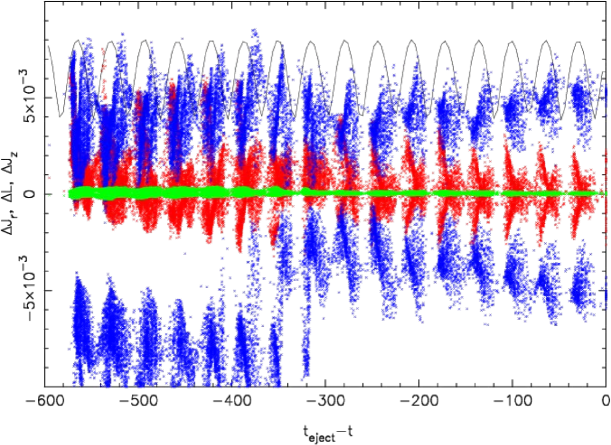
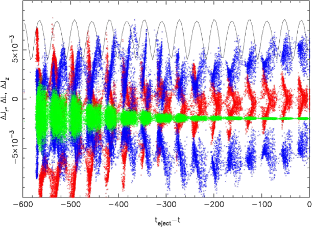
Figure 14.— The actions of stream particles relative to the satellite center for the $L/L_{c}=0.7$ satellite shown in Fig. 12, as a function of ejection time. The triaxial potentials $[a_{y},a_{z}]=[-0.05,-0.1]$ (top) and $[-0.1,-0.05]$ (bottom) contain 1000 sub-halos with 0.5% of the mass. The $\Delta J_{z}$ values are scaled down a factor of 30 to fit on the plot.

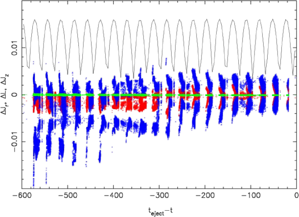
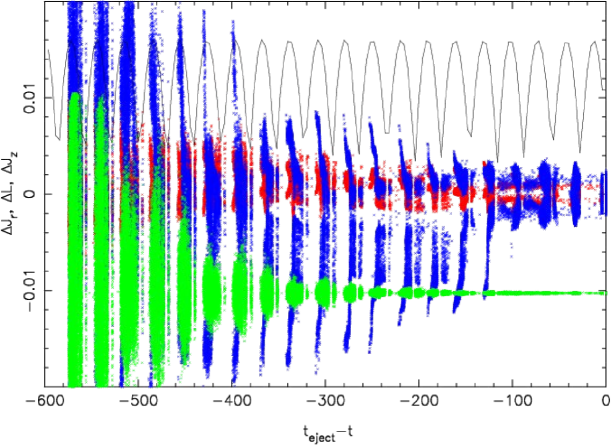
Figure 15.— Same as Figure 14 but for satellites initiated on $L/L_{c}=0.4$ orbits. Note that the vertical scale is a factor of two larger. The cluster essentially dissolves by the end of the simulation so the tidal radius is reduced for more recently lost star particles.

6. Low Eccentricity Stream Kinematics

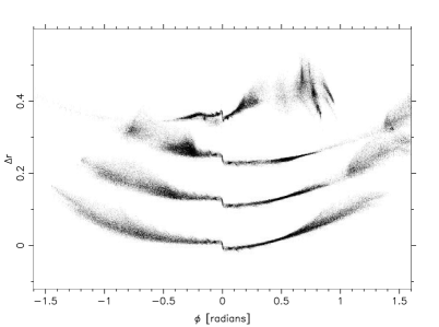
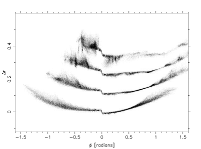
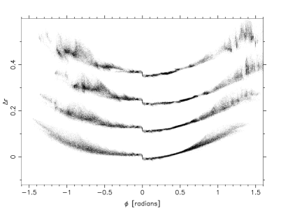
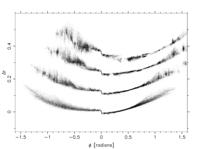
Figure 16.— The stream locations relative to radius of the orbit of the satellite, $\Delta r$ relative to the angular location of the satellite, $\phi$. The particles from satellites on $L/L_{c}=0.7$ orbits with 100, 300, 1000 and 3000 sub-halos. The mass in subhalos in each panel is 0 at the bottom then 0.2%, 0.5%, and 1% (top).

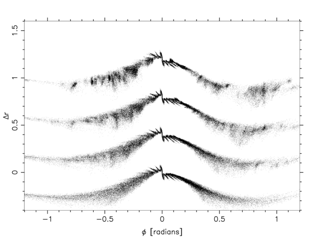
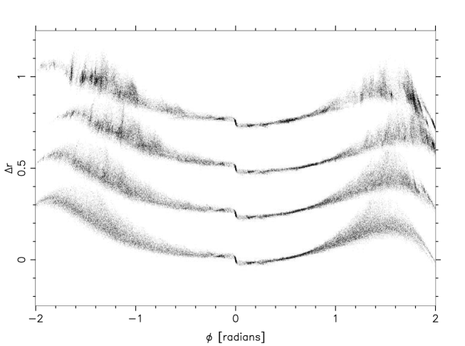
Figure 17.— The $\Delta r-\phi$ plot for a satellite ten times as massive as in Figure 16, $m=10^{-7}$ with no sub-halos at the bottom, then 1000 sub-halos with 0.2%, 0.5%, and 1% (top) of the halo mass, for time 580 (top) and 600 (bottom) to illustrate the dependence on orbital phase with a time near apocenter at the top and near pericenter at the bottom. The bottom panel is comparable to the second from the bottom panel of Figure 16 although the scales are different.

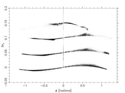
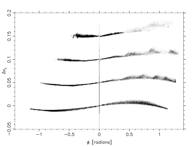
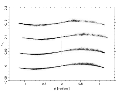
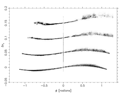
Figure 18.— Same points as Figure 16 except with the radial velocities relative to the orbital radial velocity at that angle.

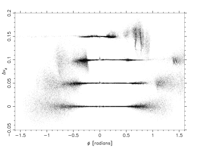
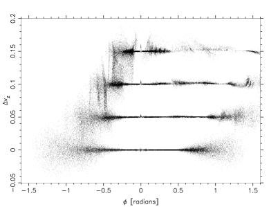
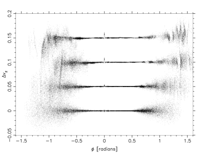
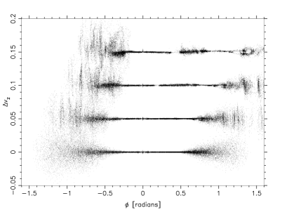
Figure 19.— Same points as Figure 16 except with the vertical velocities relative to the orbital vertical velocity at that angle.

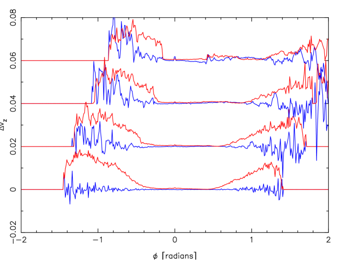
Figure 20.— The mean (blue) and dispersion (red) in vertical velocities along the stream of Figure 19 for 1000 sub-halos, with the sub-halo mass fraction rising from 0 at the bottom to 0.2, 0.5 and 1% at the top.

Low eccentricity streams have less differential shear and less morphological change with orbital phase than high eccentricity streams (Carlberg, 2015) making them better suited than high eccentricity streams as indicators of the sub-halo population of the galactic halo. Tidal streams started with $L/L_{c}=0.7$ in an $a_{y}=-0.1$, $a_{z}=-0.05$ halo with an increasing mass fraction in a varying number of sub-halos, ranging from 100 to 3000, along with zero for reference, are shown in Figures 16. The plots show the radial position of the particles relative to radius of the orbit of the center of the star cluster at that azimuthal angle. The reference orbit is calculated in the spherical isochrone potential at the end of the simulation. The figures show that the sub-halos are sufficiently numerous and massive to have significant encounters with the streams. At a 1% sub-halo mass fraction the stream is becoming so badly contorted for any of the sub-halo numbers that 1% becomes an approximate upper limit to the sub-halo fraction that can be tolerated for thin streams, although this is consistent with the predicted local fraction. With the mass entirely in 100 or 300 sub-halos the stream encounters are rarer, but have a larger effect leading to large gaps. As the sub-halos become more numerous and less massive the stream is able to large retain its basic shape, with the sub-halos producing gaps in the stream, as is most clearly seen for the 3000 sub-halo case.

The 1000 sub-halo case is repeated for a star cluster of mass $m=10^{-7}$ in Figure 17 which is ten times the cluster mass of Figure 16. The stream width and length scale with the tidal radius so are a factor of 2.15 times larger. Two snapshots are shown to illustrate the variation with orbital phase. The lower panel of Figure 17 can be compared to the second panel from the bottom of Figure 16, but note that the axes are not the same. Although the sub-halo effects remain constant, the figure also shows that sub-halo induced gaps remain visible in this slightly more than twice as wide stream from a ten times more massive progenitor cluster. Figure 17 also shows that the tidal “spurs” on the stream are much more evident particularly near apocenter as a consequence of the orbital phase dependence of the mass ejection from the satellite being initiated at pericenter with the particles drifting away at apocenter as is the case for Pal 5 (Dehnen et al., 2004).

The radial and vertical velocities of the streams emanating from the $m=10^{-8}$ cluster of Figure 16 are shown in Figures 18 and 19. The effects of increasing mass fraction in sub-halos, $f_{sh}$, over a range of $N_{sh}$ are clearly visible in the velocities of 18 and 19. In all cases the amplitude of the perturbations grows significantly with increasing $f_{sh}$ which gives a better defined “gap” along the stream. The radial velocities mix together the velocities of the tidal features and have considerable orbital phase dependence, whereas the velocities perpendicular to the orbital plane have little orbital phase dependence. The mean vertical velocity and its dispersion about the mean are shown in Figure 20. Along the stream the dispersion rises as the orbits spread out in the aspherical potential (Helmi & White, 1999; Siegal-Gaskins & Valluri, 2008; Ngan et al., 2015b). Further down the stream the stream has been out of the cluster for a longer time and has been subject to more sub-halo strikes. The mean velocity is knocked away from zero and there are local increases in the velocity dispersion. on a length scale comparable to the scale size of the dark matter halo. The Hernquist radius of the sub-halos is $0.017\sqrt[3]{(f_{sh}/0.005)(1000/N_{sh})}$. For an orbital apocenter of 30 kpc, the sub-halo radius scales to 0.13 kpc. Kinematic detection of sub-halo crossings requires enough velocity measurements per kiloparsec to be able to detect the expected velocity changes. The numbers can be worked out from simulations matched to a stream of interest, but it will be of order one hundred measurements of stream velocity per kiloparsec to be able to get started. For 0.5% of the halo mass in sub-halos, excursions around the mean velocities reach 0.02 units which is 5% of the circular velocity of 0.4 units. Or, if scaled to a circular velocity of 220  km s^-1 means that values of 11  km s^-1 are expected in the largest excursions from the mean. For 0.2% mass in sub-halos the velocity excursions are proportionally smaller. The velocity dispersion in the thin parts of the streams, which are most readily identified, is about 0.002 units, which scales to about 1 km s^-1, so these excursions should be readily detectable given enough velocities along the stream.

7. Discussion and Conclusions

We have developed a framework which is able to reproduce a large range of properties of tidal streams as are seen in galactic halos extracted from cosmological simulations. Basing the potential on the isochrone puts these simulations into a well studied regime and allows easy dynamical insight into the orbital mechanics at play. A central element of tidal stream analysis is that the distribution of star velocities in the stream can be accurately calculated, here with a spherical shell n-body code. Once free of the satellite potential, stars orbit freely, responding to in the overall potential around the orbit and the presence of sub-halos orbiting within the host potential. A question of interest is how much do the orbital actions of stream stars change relative to their initial values as a result of the asphericity of the potential and any sub-halos. If the changes are large it would diminish the value of streams as probes of the potential shape. We find that for realistic local sub-halo mass fractions of 1% or less that the orbital actions changes are about 1-2% over approximately 15-20 radial orbits. The stars most distant from the progenitor cluster are the most affected, but the changes are small enough that streams can be approximated, to this precision, as having invariant orbital actions. The outcome is a desirable situation in which sub-halos should have easily measurable local effects in velocity space, but the mean stream motions are not greatly disturbed.

Tidal streams in spherical halo models are much thinner and simpler than those seen in more realistic cosmological halos, whether there are sub-halos or not (Ngan et al., 2015b). The underlying cause is that aspherical potentials have orbits that are not present in a spherical potential, opening up more ways for the stream to spread. Near the progenitor the stream is sufficiently young that the number of sub-halo encounters is low and the stream dynamics mainly reflect the change in tidal field around the orbit. Further down the stream, where the stream has been orbiting freely longer, the cumulative effect of sub-halos and potential asphericity builds up. In the case of a high ellipticity, $e\gtrsim 0.6$, star cluster progenitor, the stream orbit spreading can be so large that the majority of the stream would be hard to identify as a high density region on they sky. However, the dense segments of high eccentricity streams certainly are visible, even though they may represent only a few percent of the entire stream, leaving the rest as a ghost. It is therefore possible that a short stream segment like Ophiuchus could be the high density region of a stream with a total luminosity a factor of ten or more larger.

Velocity measurements are the key to making progress with stream dynamics as indicators of both the shape of the halo and the substructure in the halo. It is now straightforward to reliably predict the velocity distribution of the particles newly injected into the stream, provided that the mass loss is predominantly driven by galactic tides. The presence of sub-halos leads to patches along a stream comparable in size to the characteristic radius of a sub-halo, typically 0.1-0.3 kpc, with an enhanced velocity dispersion and velocity offsets from the mean value for the stream, as shown in Figure 20. It will likely be easier to detect the mean velocity offsets along the stream, rather than local velocity dispersion increases. The large scale shape of the galactic potential leads to smooth variations along the stream. Although there already is considerable incentive to acquire spectroscopy of stars in stellar streams for abundances and orbital analysis, these simulations show that once large numbers of precision velocities are available for stream stars they will provide definitive tests for the presence of sub-halos.

This paper has concentrated on how sub-halos and triaxial potentials effect action variables, orbits and velocities and left aside an examination of gaps in streams (Yoon, Johnston & Hogg, 2011; Carlberg, 2012; Carlberg & Grillmair, 2013; Erkal & Belokurov, 2015) as indicators of the sub-halo population. Gaps will be most useful as indicators in low eccentricity streams, being blurred out fairly quickly in high eccentricity streams (Carlberg, 2015). An analysis of gaps and velocity offsets in these streams as sub-halo indicators will be presented elsewhere.

References

- Aarseth (1967) Aarseth, S. 1967, Les Nouvelles Méthodes de la Dynamique Stellaire, 47
- Amorisco (2014) Amorisco, N. C. 2015, MNRAS, 450, 575
- Bernard et al. (2014) Bernard, E. J., Ferguson, A. M. N., Schlafly, E. F., et al. 2014, MNRAS, 443, L84
- Binney (2008) Binney, J. 2008, MNRAS, 386, L47
- Binney & Tremaine (2008) Binney, J., & Tremaine, S. 2008, Galactic Dynamics: Second Edition, Princeton University Press
- Binney (2014) Binney, J. 2014, MNRAS, 440, 787
- Bonaca et al. (2014) Bonaca, A., Geha, M., Kuepper, A. H. W., et al. 2014, arXiv:1406.6063
- Bovy (2014) Bovy, J. 2014, ApJ, 795, 95
- Brockamp et al. (2014) Brockamp, M., Küpper, A. H. W., Thies, I., Baumgardt, H., & Kroupa, P. 2014, MNRAS, 441, 150
- Carlberg (2012) Carlberg, R. G. 2012, ApJ, 748, 20
- Carlberg & Grillmair (2013) Carlberg, R. G., & Grillmair, C. J. 2013, ApJ, 768, 171
- Carlberg (2015) Carlberg, R. G. 2015, ApJ, 800, 133
- Dehnen et al. (2004) Dehnen, W., Odenkirchen, M., Grebel, E. K., & Rix, H.-W. 2004, AJ, 127, 2753
- Diemand, Kuhlen & Madau (2007) Diemand J., Kuhlen M., Madau P., 2007, ApJ, 667, 859
- de Zeeuw (1985) de Zeeuw, T. 1985, MNRAS, 216, 273
- Erkal & Belokurov (2015) Erkal, D., & Belokurov, V. 2015, MNRAS, 450, 1136
- Eyre & Binney (2011) Eyre, A., & Binney, J. 2011, MNRAS, 413, 1852
- Fardal et al. (2014) Fardal, M. A., Huang, S., & Weinberg, M. D. 2014, arXiv:1410.1861
- Fry & Peebles (1980) Fry, J. N., & Peebles, P. J. E. 1980, ApJ, 236, 343
- Fujii et al. (2007) Fujii, M., Iwasawa, M., Funato, Y., & Makino, J. 2007, PASJ, 59, 1095
- Fukushige & Heggie (2000) Fukushige, T., & Heggie, D. C. 2000, MNRAS, 318, 753
- Giersz (2006) Giersz, M. 2006, MNRAS, 371, 484
- Grillmair & Dionatos (2006) Grillmair, C. J., & Dionatos, O. 2006, ApJ, 643, L17
- Helmi & White (1999) Helmi, A., & White, S. D. M. 1999, MNRAS, 307, 495
- Henon (1959a) Henon, M. 1959, Annales d’Astrophysique, 22, 126
- Henon (1959b) Henon, M. 1959, Annales d’Astrophysique, 22, 491
- Hénon (1960) Hénon, M. 1960, Annales d’Astrophysique, 23, 474
- Hernquist (1990) Hernquist, L. 1990, ApJ, 356, 359
- Hernquist & Ostriker (1992) Hernquist, L., & Ostriker, J. P. 1992, ApJ, 386, 375
- Hozumi & Burkert (2015) Hozumi, S., & Burkert, A. 2015, MNRAS, 446, 3100
- Ibata et al. (2002) Ibata, R. A., Lewis, G. F., Irwin, M. J., & Quinn, T. 2002, MNRAS, 332, 915
- Johnston et al. (1996) Johnston, K. V., Hernquist, L., & Bolte, M. 1996, ApJ, 465, 278
- Johnston (1998) Johnston, K. V. 1998, ApJ, 495, 297
- Johnston et al. (1999) Johnston, K. V., Zhao, H., Spergel, D. N., & Hernquist, L. 1999, ApJ, 512, L109
- King (1966) King, I. R. 1966, AJ, 71, 64
- Klypin et al. (1999) Klypin, A., Kravtsov, A. V., Valenzuela, O., & Prada, F. 1999, ApJ, 522, 82
- Küpper et al. (2008) Küpper, A. H. W., MacLeod, A., & Heggie, D. C. 2008, MNRAS, 387, 1248
- Küpper et al. (2012) Küpper, A. H. W., Lane, R. R., & Heggie, D. C. 2012, MNRAS, 420, 2700
- Louis & Gerhard (1988) Louis, P. D., & Gerhard, O. E. 1988, MNRAS, 233, 337
- Meiron et al. (2014) Meiron, Y., Li, B., Holley-Bockelmann, K., & Spurzem, R. 2014, ApJ, 792, 98
- McGlynn (1984) McGlynn, T. A. 1984, ApJ, 281, 13
- McGlynn (1990) McGlynn, T. A. 1990, ApJ, 348, 515
- Moore et al. (1999) Moore B., Ghigna S., Governato F., et al., 1999a, ApJL, 524, L19
- Ngan & Carlberg (2014) Ngan, W. H. W., & Carlberg, R. G. 2014, ApJ, 788, 181
- Ngan et al. (2015a) Ngan, W., Bozek, B., Carlberg, R. G., et al. 2015, ApJ, 803, 75
- Ngan et al. (2015b) Ngan, W., Carlberg, R. G., Bozek, B. et al. 2015, in preparation
- Odenkirchen et al. (2001) Odenkirchen, M., Grebel, E. K., Rockosi, C. M., et al. 2001, ApJ, 548, L165
- Pearson et al. (2015) Pearson, S., Küpper, A. H. W., Johnston, K. V., & Price-Whelan, A. M. 2015, ApJ, 799, 28
- Sesar et al. (2015) Sesar, B., Bovy, J., Bernard, E. J., et al. 2015, arXiv:1501.00581
- Siegal-Gaskins & Valluri (2008) Siegal-Gaskins, J. M., & Valluri, M. 2008, ApJ, 681, 40
- Springel (2005) Springel, V. 2005, MNRAS, 364, 1105
- Springel et al. (2008) Springel, V. et al. 2008, MNRAS, 391, 1685
- Sollima & Mastrobuono Battisti (2014) Sollima, A., & Mastrobuono Battisti, A. 2014, MNRAS, 443, 3513
- Stadel et al. (2009) Stadel, J., Potter, D., Moore, B., et al. 2009, MNRAS, 398, L21
- Varghese et al. (2011) Varghese, A., Ibata, R., & Lewis, G. F. 2011, MNRAS, 417, 198
- van Albada & van Gorkom (1977) van Albada, T. S., & van Gorkom, J. H. 1977, A&A, 54, 121
- Villumsen (1982) Villumsen, J. V. 1982, MNRAS, 199, 493
- White (1983) White, S. D. M. 1983, ApJ, 274, 53
- Yoon, Johnston & Hogg (2011) Yoon, J. H., Johnston, K. V., & Hogg, D. W. 2010, ApJ, 731, 58