Stochastic amplification of weak signals in an RF SQUID with ScS contact

Abstract

The paper presents results of a numerical simulation of the stochastic dynamics of magnetic flux in an RF SQUID loop with a Josephson point (ScS) contact driven by a mix of band-limited Gaussian noise and low-frequency small-amplitude sine signal, at finite temperatures $0<T<T_{c}$. A change in the gain of the stochastically amplified weak signal with the temperature rise is shown to be due to smearing of the energy barrier between adjacent metastable current states of the loop. A comparison to an RF SQUID with a tunnel (SIS) junction is done.

I Introduction

The magnetometers based on Superconducting Quantum Interference Devices (SQUIDs) are widely used in physical experiments, medicine (magnetocardiographs and magnetoencephalographs), geophysics (underground radars), electronic manufacturing (SQUID microscopes). The sensitivity of SQUIDs and their quantum analogues, SQUBIDs, has practically reached the quantum limitation 1Ketchen ; 2Shnyrkov ; 3Shnyrkov . However, with increase of the quantizing loop inductance up to $L\sim 10^{-9}-10^{-10}\;H$ , the thermodynamic fluctuations lead to expressed degradation of the energy resolution.

As shown earlier 4Rouse ; 5Hibbs ; 6Turutanov ; 7Glukhov , the sensitivity of the magnetometers can be considerably enhanced in this case by using the stochastic resonance (SR) effect. The SR phenomenon discovered in the early 1980s 8Benzi ; 9Nicolis manifests itself in a non-monotonic rise of a nonlinear (often bi-stable) system response to a weak periodic signal which peaks at a certain intensity of the noise added (or inherent) to the system.

Owing to extensive studies during the last two decades, the stochastic resonance effect has been revealed in a variety of natural and artificial systems, both classical and quantum ones. Analytical approaches and quantifying criteria for estimation of the noise-induced ordering were determined and then summarized in the reviews 10Gammaitoni ; 11Anishchenko . For example, the gain of 40 dB was experimentally demonstrated 4Rouse for a weak harmonic signal due to SR in a SQUID with the tunnel (SIS) Josephson junction. For an under-optimal noise intensity, the signal gain in SR SQUIDs can be nevertheless maximized with the stochastic-parametric resonance (SPR) effect 12Turutanov emerging when the system is affected by the weak signal, the noise and an additional high-frequency electromagnetic field simultaneously.

Not so long ago, researchers paid their attention to clean small-sized superconducting contacts of ”constriction” (ScS) type called the ”atomic-size contacts”, ASCs 13Agrait . They have only a few quantum conductive channels in their cross section so they often referred to as the ”quantum point contacts”, QPCs 14Beenakker . The critical current $I_{c}$ of such contacts may take discrete values. The interest to the QPCs is roused by studies of the channel quantum conductivity and building superconducting qubits with large energy level splitting $\Delta E/h\sim 30\;GHz$ 2Shnyrkov . The current-phase relation (the supercurrent $I_{s}$ as a function of the order parameter phase difference $\varphi$ ) in the clean ScS contacts with ballistic electron transit at low temperatures ( $T\to 0$ ) 14Beenakker ; 15Kulik substantially differs from the classical Josephson current-phase relation for a SIS junction $I_{s}^{SIS}(\varphi)=I_{c}\sin\varphi$ and features a ”saw-like” shape with discontinuities at $\varphi=n\pi$.

The coupling energies for SIS and ScS obtained by integrating the current-phase relations therefore differ, too. If the SIS junction is incorporated into a superconducting loop and an external magnetic flux $\Phi_{e}=\Phi_{0}/2$ is applied ( $\Phi_{0}=h/2e\approx 2.07\cdot 10^{-15}\;Wb$ is the magnetic flux quantum), its current-phase relation forms the symmetric two-well potential of the loop, which is needed for SR, only at sufficiently large loop inductances and/or the junction critical current, namely, when $\beta_{L}=2\pi LI_{c}/\Phi_{0}>1$ . Unlikely, the potential energy $U^{ScS}(\Phi)$ of the superconducting loop with a QPC has a ”sharp” barrier with the singularity in its top separated two metastable current-carrying states of the loop with different intrinsic magnetic flux $\Phi$ for any $\beta_{L}$ including $\beta_{L}<<1$.

In classical case for the zero-temperature limit, the stochastic dynamics of the magnetic flux in a superconducting loop with the Josephson ScS contact (ScS SQUID) substantially differs from that for SIS SQUID studied earlier 4Rouse ; 5Hibbs ; 7Glukhov . Taking into account the quantum fluctuations at finite temperatures $0<T<T_{c}$ changes the current-phase relation for the ScS contact and smoothes the potential barrier in the loop with ScS contact 17Khlus . In this work we analyze the stochastic amplification of weak low-frequency harmonic signals in a superconducting loop interrupted by Josephson ScS contact, at finite temperatures and various $\beta_{L}$. The results are compared with the stochastic dynamics of a SIS SQUID.

II Model

The stochastic dynamics of the magnetic flux inside an RF SQUID loop (inset in Fig. 1) is studied by numerical solving the motion equation (Langevin equation) in the model of resistively shunted junction (RSJ model):

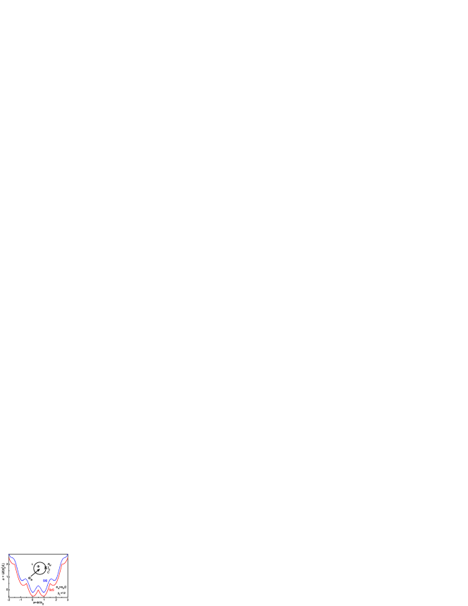
Figure 1: The potential energy of RF SQUID loop with ScS contact (solid line) and SIS junction (dotted line) as a function of reduced magnetic flux in the loop. The non-linearity parameter $\beta_{L}=12$, fixed external magnetic flux $\Phi_{e}=\Phi_{0}/2$. The inset shows schematically the RF SQUID loop with a Josephson junction, the designations are described in the text.

$$LC\frac{d^{2}\Phi(t)}{dt^{2}}+\frac{L}{R_{N}}\frac{d\Phi(t)}{dt}+L\frac{dU(\Phi)}{d\Phi}=\Phi_{e}(t),$$ (1)

where $C$ is the capacitance, $R_{N}$ and $I_{c}$ are the normal shunt resistance and the critical current of the Josephson junction, respectively, $\Phi(t)$ is the magnetic flux inside loop, $U(\Phi,\Phi_{e})$ is the loop potential energy of the which is the sum of the loop magnetic energy $U_{M}$ and the Josephson junction coupling energy $U_{J}$. The time-dependent external magnetic flux $\Phi_{e}(t)$ applied to the loop contains the fixed and the varying components including the noise one. The junction coupling energy $U_{J}$ is type-determined (for SIS, ScS, SNS, etc.). The potential energy of a loop with the ”traditional” tunnel (SIS) junction is equal to 18Barone

$$U^{SIS}(\Phi,\Phi_{e})=\frac{(\Phi-\Phi_{e})^{2}}{2L}-E_{J}^{SIS}\cos\frac{2\pi\Phi}{\Phi_{0}},$$ (2)

where $E_{J}^{SIS}=I_{c}\Phi_{0}/2\pi$ is maximal coupling energy of the tunnel Josephson junction.

We consider the dynamics of the magnetic flux in the RF SQUID loop incorporating the clean ScS contact with ballistic electron transit 15Kulik .

For classical 15Kulik and quantum 14Beenakker ScS contacts with the critical current $I_{c}$ the current-phase relation in the zero-temperature limit $T=0$

$$I_{S}^{ScS}(\varphi)=I_{c}(\sin\frac{\varphi}{2})\,sgn\,(\cos\frac{\varphi}{2})$$ (3)

has the ”saw-like” shape with discontinuities at $\varphi=n\pi$. Correspondingly, the potential energy of the superconducting loop with ScS contact is

$$U^{ScS}(\Phi,\Phi_{e})=\frac{(\Phi-\Phi_{e})^{2}}{2L}-E_{J}^{ScS}\left|\cos\frac{\pi\Phi}{\Phi_{0}}\right|,$$ (4)

where $E_{J}^{ScS}=I_{c}\Phi_{0}/\pi$ is the maximal coupling energy of the Josephson ScS contact. $U^{ScS}(\Phi,\Phi_{e})$ has singularities in tops of the barriers separating the adjacent local minima which correspond to the loop metastable current states.

Introducing the dimensionless parameter of non-linearity

$$\beta_{L}=2\pi LI_{c}/\Phi_{0},$$ (5)

and reducing the fluxes by the flux quantum $\Phi_{0}$: $x=\Phi/\Phi_{0}$ , $x_{e}=\Phi_{e}/\Phi_{0}$, and the potential energy by $\Phi_{0}^{2}/2L$, expressions (2) and (4) can be rewritten, correspondingly, as

$$u^{SIS}(x,x_{e})=\frac{(x-x_{e})^{2}}{2}-\frac{\beta_{L}}{4\pi^{2}}\cos 2\pi x$$ (6)

and

$$u^{ScS}(x,x_{e})=\frac{(x-x_{e})^{2}}{2}-\frac{\beta_{L}}{2\pi^{2}}\left|\cos\pi x\right|.$$ (7)

The potential energy $u^{SIS}(x,x_{e})$ of the loop with a tunnel junction has two or more local minima only at $\beta_{L}>1$. It can be symmetrized by applying fixed magnetic field $\Phi_{e}=\Phi_{0}/2\;\;(x_{e}=1/2)$ . Fig. 1 shows potential energy of the loops with SIS and ScS contacts as a function of internal magnetic field at large $\beta_{L}=12$ for better visibility. The distinctive feature of the potential energy $u^{ScS}(x,x_{e})$ of an RF SQUID loop with the ScS contact is the finite height of the ”sharp” barrier between adjacent states for any vanishingly small $\beta_{L}$, i.e. $L$ and/or $I_{c}$ (at zero temperature). Fig. 2 displays potential energies of the RF SQUIDs with SIS or ScS contact at several small $\beta_{L}$. It is obvious from Fig. 2 that the barrier separating the two metastable current-carrying states vanishes at $\beta_{L}=1$ in the SIS SQUID while stays finite in the ScS SQUID.

Figure 2: The potential energy of the ScS (solid line) and SIS (dashed line) SQUIDs as a function of internal reduced magnetic flux for several $\beta_{L}$ . The fixed external flux $\Phi_{e}=\Phi_{0}/2$ . The barrier height $\Delta U$ and the inter-minima spacing $\Delta x$ are shown in the curves for $\beta_{L}=1.5$ .

The noise of thermal or any other origin causes switching between the metastable states corresponding to the minima of $U(\Phi)$ . The switching rate for the white Gaussian noise with intensity (variance) $D$ for parabolic wells and $\Delta U/D>>1$ is given by the Kramers’ formula 19Kramers :

$$r_{K}=r_{0}\exp(-\Delta U/D).$$ (8)

In the case of thermal noise for $T=0$ , $D=2k_{B}T$. In this work we do not focus on any specific nature of the noise. The only requirement imposed to ensure the adiabatic mode of the SQUID switching is the limitation of the noise frequency band by a frequency not exceeding the reciprocal relaxation time for the internal flux in the SQUID loop $1/\tau_{L}=R/L$. Although the pre-exponential factor $r_{0}$ is different for the ”smooth” potential of the SIS SQUID and ”sharp” potential of the ScS SQUID (details can be found in 16Turutanov ), the exponent factor dominates anyway. Adding a small periodic signal with frequency $f_{s}$ to the external flux $\Phi_{e}$ results in the stochastic-resonance system motion in the noise-driven bistable potential at

$$r_{K}\approx 2f_{s}.$$ (9)

Taking typical experimental figures $L=3\cdot 10^{-10}\;H$, $C=3\cdot 10^{-15}\;F$, $R_{N}=1...10^{2}\;\Omega$, $I_{c}=10^{-5}...10^{-6}\;A$, we found the McCamber parameter describing the effect of capacitance $\beta_{C}=2\pi R^{2}I_{c}C/\Phi_{0}<1$. This case corresponds to the viscous, non-oscillatory, motion and therefore the term with the second derivative in Eq. (1) can be neglected. Low signal frequency $f_{s}=10\;Hz<<1/\tau_{L}$ and noise cut-off frequency $f_{c}\sim 10^{4}\;Hz<<1/\tau_{L}$ makes the problem adiabatic. This allows us the time dependence of the external flux consider as the time-dependent potential energy thus writing the motion equation in the form

$$\tau_{L}\frac{dx}{dt}+\frac{\partial u(x,t)}{\partial x}=0.$$ (10)

With (6) for the SIS junction, the Eq. (10) reads as

$$\frac{dx}{dt}=\frac{1}{\tau_{L}}[x_{e}(t)-x+\frac{\beta_{L}}{4\pi}\sin 2\pi x],$$ (11)

and with (7) for the ScS contact, as

$$\frac{dx}{dt}=\frac{1}{\tau_{L}}[x_{e}(t)-x+\frac{\beta_{L}}{2\pi}(\sin\pi x)\,sgn\,(cos\pi x)].$$ (12)

The external flux $x_{e}(t)$ is the sum of the fixed bias flux $x_{dc}=0.5$, the useful signal $x_{ac}=a\sin 2\pi f_{s}t$ and the noise flux $x_{N}$. In the theory, the noise is often treated as the $\delta$-correlated white, Gaussian-distributed noise: $x_{N}=\xi(t)$, $\left\langle\xi(t)\cdot\xi(t-t^{\prime})\right\rangle=2D\delta(t-t^{\prime})$. During the numerical simulation, it is modeled by the quasi-random number generator giving Gaussian-distributed values with variance $D=\sigma^{2}$ and the repetition period of about $2^{90}$. The sampling rate is $2^{16}$ when solving the equation by finite differences technique that corresponds to the equivalent noise frequency band 32 kHz. So, the noise can be considered as quasi-white for the stochastic amplification of the signal with frequency $f_{s}=10\;Hz$.

Eqs. (11) and (12) were solved by the Heun method modified for the stochastic equations 20Garcia . Each run gave an 8-s-long time series with its individual noise realization and then were subjected to fast Fourier transform (FFT). The obtained output spectral densities $S_{\Phi}(\omega)$ of the internal flux were averaged over 30 runs. The spectral amplitude gain of the weak periodic signal was determined as the ration of spectral densities of the input (external) and output (internal) magnetic fluxes:

$$k(\omega)=S_{\Phi\;out}^{1/2}(\omega)/S_{\Phi\;in}^{1/2}(\omega).$$ (13)

III Results and discussion

The current-phase relation for the ScS contact at a non-zero temperature $T$ 14Beenakker ; 15Kulik

$$I_{s}^{ScS}(\varphi)=I_{c}\sin\frac{\varphi}{2}\tanh\frac{\Delta(T)\cos\frac{\varphi}{2}}{2k_{B}T},$$ (14)

where $I_{s}^{ScS}(\varphi)$ is the contact supercurrent, $I_{c}=\frac{\pi\Delta(T)}{eR_{N}}$ is the contact critical current, $\Delta(T)$ is the superconductor energy gap (order parameter), $\varphi$ is the order parameter phase difference over the contact, $k_{B}$ is the Boltzmann constant, $e$ is the electron charge, $R_{N}$ is the contact normal resistance, smoothes, tending, as approaching the superconductor critical temperature $T_{c}$, to the sine law that describes the SIS junction. Consequently, the (reduced) potential energy of the loop with ScS contact

$$u_{T}^{ScS}=\frac{(x-x_{e})^{2}}{2}-\frac{\beta_{L}}{\pi^{2}}t\ln\left(2\cosh\frac{\cos\pi x}{2t}\right),$$ (15)

where $t=\frac{T/T_{c}}{1.76\sqrt{1-(T/T_{c})^{4}}}$, also becomes closer in its shape to the SIS SQUID potential energy. The singularity in the barrier top disappears, while the barrier height decreases with the temperature rise. Fig. 3 illustrates the temperature evolution of ScS SQUID potential energy. The SIS SQUID potential energy is also given in the Figure for the comparison sake. In contrary to the zero-temperature case, the potential barrier vanishes at a certain reduced temperature even for $\beta_{L}>1$ (at $T/T_{c}=0.5$ for the chosen $\beta=1.2$) The inter-minima spacing decreases, too. The barrier heights for the ScS- and SIS-SQUIDs become equal at a certain temperature (at $T/T_{c}=0.375$ for the given case).

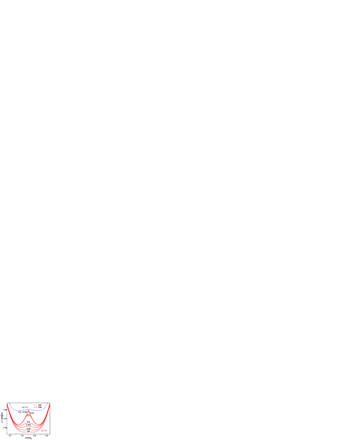
Figure 3: The potential energy of ScS SQUID as a function of the magnetic flux in the loop at various reduced temperatures. Similar function for the SIS SQUID at the same $\beta_{L}$ is shown for comparison.

By substituting (15) in(10), we get the motion equation for the reduced flux in ScS SQUID at finite temperatures $T$ , $0<T<T_{c}$ , similar to Eq. (11) for the case $T=0$. The solution of this equation at various noise intensities with further FFT as described above gives the spectral gain of a weak signal as a function of the noise intensity, i.e. the SR curves.

Fig. 4 shows the SR curves in the ScS SQUID calculated for several reduced temperatures and $\beta_{L}=1.21$. Strictly saying, $\beta_{L}$ parameter is indicated for $T=0$, since it renormalizes as the temperature rises. For the comparison, the SR curve in a SIS SQUID loop is displayed in the figure for the same $\beta_{L}$. One can see that, with the temperature rise, the maximal gain in ScS SQUID increases due to lowering of the barrier. This is much like a SIS SQUID behavior when $\beta_{L}$ reduces down to the unity 16Turutanov , so we consider the situation as a ”renormalization” of $\beta_{L}$ in ScS SQUIDs.

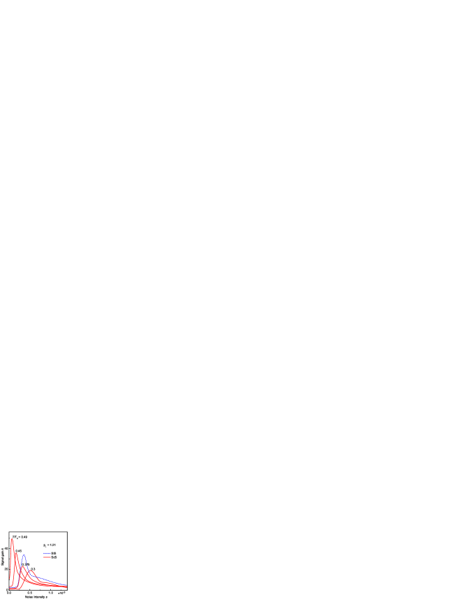
Figure 4: The weak harmonic signal gain as a function the noise intensity in SIS and ScS SQUIDs at various reduced temperatures. The signal amplitude is 0.001, frequency 10 Hz.

When the barriers in the ScS and SIS SQUIDs are of the same height ($T/T_{c}=0.375$, see Fig. 3), the maximal gain is observed at equal noise intensities for both SQUIDs while the maximal gain values are different because of difference in the potential shapes and inter-minima spacings $\Delta x$ 16Turutanov .

According to the two-state theory for linear response 21McNamara which does not accounts for inter-well dynamics, the weak-signal gain is determined by the spacing $\Delta x$ between the adjacent local minima of the system potential energy. Taking the SR curves in Fig. 4 for ScS and SIS SQUIDs with almost equal maximal gain ( $T/T_{c}=0.45$ for ScS SQUID) and looking up corresponding potential energies in Fig. 4, we can see that $\Delta x$ values are somewhat different. This implies that the exact shapes of the potential profile should be involved in accurate theoretical calculation. Nevertheless, it can be generally stated that the stochastic amplification of an informational signal in ScS SQUIDs with small $\beta_{L}$ will reveal its specific features at ultra-low temperatures. The calculation shows the potential barrier in ScS SQUID with $\beta_{L}=0.1$ vanishes at $T/T_{c}=0.045$ , that for niobium with its critical temperature $T_{c}=9.25\;K$ corresponds to a millikelvin temperature range. At such low temperatures, quantum effects will give a dominant contribution in switching rate 22Grifoni . Moreover, the ”sharp” potential of a superconducting loop with ScS contact makes quantum tunneling between separated wells much faster as compared to a ”common” SIS circuit. This feature allowed authors of 2Shnyrkov to propose a superconducting qutrit-detector with tunneling rate of 20-30 GHz (which was important there for large energy level splitting). Thus, an interesting situation could emerge in ScS SQUIDs at ultra-low temperatures when two characteristic time scales would occur in the context of stochastic resonance, one for classical hops over the barrier and other for quantum tunneling through it.

IV Conclusion

The calculation of amplification of a weak harmonic signal on a noisy background due to the stochastic resonance in an RF SQUID loop with a clean ScS contact in the zero-temperature limit shows that the SR in ScS SQUID is possible at any vanishingly small $\beta_{L}<1$ because of unusual ”sharp” potential barrier between metastable states whose height is always finite at $T=0$.

With the ScS SQUID temperature rise, the top of the barrier smoothes, its height gradually vanishes to zero, and the potential of the ScS SQUID becomes much like that of ”common” SIS SQUID. Thus, the substantial difference in classic stochastic dynamics of magnetic flux of ScS and SIS SQUIDs emerge at ultra-low temperatures. The difference will become more distinctive if quantum tunneling contribution is taken into account. These distinctions should be considered, as useful or ”parasitic” effect, in designing deep-cooled devices involving superconducting loops with incorporated Josephson junctions, such as SQUIDs and qubits.

References

- (1) M.B. Ketchen, J.M. Jaycox, Appl. Phys. Lett. 40, 736 (1982).
- (2) V.I. Shnyrkov, A.A. Soroka, and O.G. Turutanov, Phys. Rev. B85, 224512 (2012).
- (3) V.I. Shnyrkov, A.A. Soroka, A.M. Korolev, O.G. Turutanov, J. Low Temp. Phys. 38, 301 (2012).
- (4) R.Rouse, Siyuan Han, J.E. Lukens, Appl. Phys. Lett. 66, 108 (1995).
- (5) A.D. Hibbs, A.L. Singsaas, E.W. Jacobs, A.R. Bulsara, J.J. Bekkedahl et al., J. Appl. Phys. 77, 2582 (1995).
- (6) O.G. Turutanov, A.N. Omelyanchouk, V.I. Shnyrkov, Yu.P. Bliokh, Physica C 372-376, 237-239 (2002).
- (7) A.M. Glukhov, O.G. Turutanov, V.I. Shnyrkov, A.N. Omelyanchouk, J. Low Temp. Phys. 32 (2006) 1123.
- (8) R. Benzi, A. Sutera, A. Vulpiani, J. Phys. A14, L453 (1981).
- (9) C. Nicolis, G. Nicolis, Tellus 33, 225 (1981).
- (10) L. Gammaitoni, P. Hänggi, P. Jung, F. Marchesoni, Rev. Mod. Phys. 70, 223 (1998).
- (11) V.S. Anishchenko, A.B. Neiman, F. Moss, L. Schimansky-Geier, Phys. -Usp. 42 (1999) 7.
- (12) O.G. Turutanov, V.I. Shnyrkov, A.M. Glukhov, J. Low Temp. Phys. 34 (2008) 37.
- (13) N. Agraït, A. L. Yeyati, and J. M. van Ruitenbeek, Phys. Rep.377, 81 (2003).
- (14) C.W. J. Beenakker, H. van Houten, Phys. Rev. Lett. 66, 3056 (1991); in Nanostructures and Mesoscopic Systems, ed. by W.P. Kirk and M.A. Reed, Academic, New York, 1992, p. 481; arXiv:cond-mat/0512610.
- (15) I.O. Kulik, A.N. Omelyanchouk, Sov. J. Low Temp. Phys. 3, 459 (1977).
- (16) O.G. Turutanov, V.A. Golovanevskiy, V.Yu. Lyakhno, V.I. Shnyrkov, Physica A 396, 1 (2014)
- (17) V.A. Khlus, Sov. J. Low Temp. Phys. 12 (1986) 14
- (18) A. Barone, G. Paterno, Physics and Applications of the Josephson Effect, Wiley, New York, 1982.
- (19) H.A. Kramers, Physica 7, 284 (1940).
- (20) J. L. Garcia-Palacios, Introduction to the theory of stochastic processes and Brownian motion problems, cond-mat/0701242 (January 2007); Peter E. Kloeden, Eckhard Platen, Numerical Solution of Stochastic Differential Equations, 632 pp., Springer (1992).
- (21) B. McNamara, K. Wiesenfeld, Phys.Rev. A 39, 4854 (1989).
- (22) M. Grifoni, L. Hartmann, S. Berchtold, P. Hanggi, Phys. Rev. E 53 (1996) 5890.