Triangular Fully Packed Loop Configurations of Excess 2

Abstract.

Triangular fully packed loop configurations (TFPLs) came up in the study of fully packed loop configurations on a square (FPLs) corresponding to link patterns with a large number of nested arches. To a TFPL is assigned a triple $(u,v;w)$ of $01$-words encoding its boundary conditions which must necessarily satisfy that $d(u)+d(v)\leq d(w)$, where $d(u)$ denotes the number of inversions in $u$. Wieland gyration, on the other hand, was invented to show the rotational invariance of the numbers $A_{\pi}$ of FPLs corresponding to a given link pattern $\pi$. Later, Wieland drift – a map on TFPLs that is based on Wieland gyration – was defined. The main contribution of this article is a linear expression for the number of TFPLs with boundary $(u,v;w)$ where $d(w)-d(u)-d(v)=2$ in terms of numbers of stable TFPLs, that is, TFPLs invariant under Wieland drift. This linear expression is consistent with already existing enumeration results for TFPLs with boundary $(u,v;w)$ where $d(w)-d(u)-d(v)=0,1$.

1. Introduction

The basis for this article is the fully packed loop model that has its origin in the six-vertex model (which is also called square ice model) of statistical mechanics; a fully packed loop configuration (FPL) of size $n$ is a subgraph $F$ of the $n\times n$-square grid together with $2n$ external edges such that each of the $n^{2}$ vertices is of degree $2$ in $F$ and every other external edge is occupied by $F$ starting with the topmost horizontal external edge on the left side. See Figure 1 for an example.

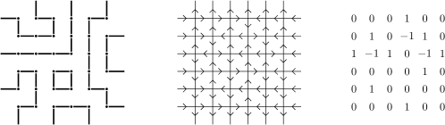
Figure 1. An FPL, a six vertex configuration and an ASM.

FPLs are significant to algebraic combinatorics due to their one-to-one correspondence to alternating sign matrices (ASMs). This is why FPLs of size $n$ are enumerated by the famous formula for the number of ASMs of size $n$ proved in [13].

In contrast to alternating sign matrices, FPLs allow a refined study in dependency on the connectivity of the occupied external edges (these connections are encoded as a link pattern). The study of FPLs having a link pattern with nested arches is an example of one such refined study; it was conjectured in [14] and later proved in [4] that the number of FPLs having a fixed link pattern $\pi\cup m$ consisting of a link pattern $\pi$ of size $n$ and $m$ nested arches is polynomial in $m$. In the course of the proof of this conjecture triangular fully packed loop configurations (TFPLs) came up. To be more precise, the following expression for the number $A_{\pi}(m)$ of FPLs having link pattern $\pi\cup m$ including numbers $t_{u,v}^{w}$ of TFPLs satisfying certain boundary conditions encoded by a triple $(u,v;w)$ of $01$-words was shown:

(1.1) $$A_{\pi}(m)=\sum\limits_{u,v\in\mathcal{D}_{n}}P_{\lambda(u)}(n)t_{u^{\prime},v^{\prime}}^{\textbf{w}(\pi)}P_{\lambda(v)^{\prime}}(m-2n+1),$$

where the sum runs over all Dyck words $u,v$ of length $2n$, $u^{\prime}$ denotes the $01$ word obtained from a Dyck word $u$ by deleting the first $0$ and the last $1$, $\textbf{w}(\pi)$ denotes the Dyck word corresponding to the link pattern $\pi$, $\lambda(u)$ denotes the Young diagram associated with a $01$ word $u$, $\lambda^{\prime}$ denotes the conjugate of a Young diagram $\lambda$ and

$$P_{\lambda}(x)=\prod\limits_{\mathfrak{C}\in\lambda}\frac{x+c(\mathfrak{C})}{h(\mathfrak{C})}$$

with $c(\mathfrak{C})$ being the content of the cell $\mathfrak{C}$ and $h(\mathfrak{C})$ the hook length of $\mathfrak{C}$. Apperantly, Equation (1.1) motivates the study of TFPLs and the numbers $t_{u,v}^{w}$. Another motivation for their study comes from the many nice properties of TFPLs which have been discovered since the emergence of TFPLs, see [11], [8] and [5]. An example of one such property is that the boundary $(u,v;w)$ of a TFPL has to fulfill that $d(u)+d(v)\leq d(w)$, where $d(\omega)$ denotes the number of inversions in a word $\omega$; the integer

$$\operatorname{exc}(u,v;w)=d(w)-d(u)-d(v)$$

is said to be the excess of $u,v,w$. To study TFPLs with respect to the excess of their boundary turned out to be fruitful; in [5] enumeration results for TFPLs with boundary $(u,v;w)$ where $exc(u,v;w)=0,1$ were proved.

Figure 2. A triangular fully packed loop configuration with boundary $(0000111,1010010;1100100)$.

Wieland gyration, on the other hand, is an operation on FPLs that was invented in [12] to prove the rotational invariance of the numbers $A_{\pi}$ of FPLs corresponding to given link patterns $\pi$. Later it was heavily used by Cantini and Sportiello [3] to prove the Razumov–Stroganov conjecture. In connection with TFPLs, Wieland gyration first appeared in [8] following work of [11], after which Wieland drift was introduced in [1] as the natural definition of Wieland gyration for TFPLs. In contrast to Wieland gyration, Wieland drift is not an involution. It was shown in [1] that Wieland drift is eventually periodic with period $1$.

This article will focus on TFPLs with boundary $(u,v;w)$ where $exc(u,v;w)=2$. The main contribution of this paper will be a linear expression for $t_{u,v}^{w}$ in terms of numbers of stable TFPLs, that is, TFPLs invariant under the application of Wieland drift. This linear expression is consistent with the already existing enumeration results for TFPLs with boundary $(u,v;w)$ where $exc(u,v;w)=0,1$.

To give the exact formulation of the main result of this article further notation is needed: let $\sigma$ and $\tau$ be two $01$-words of length $N$. Then

• $|\omega|_{i}$ will denote the number of occurrences of $i$ in $\sigma$;

• it will be written $\sigma\leq\tau$ if $|\sigma_{1}\cdots\sigma_{m}|_{1}\leq|\tau_{1}\cdots\tau_{m}|_{1}$ for all $1\leq m\leq N$;

• $\overleftarrow{\sigma}$ will denote the word $\sigma_{N}\cdots\sigma_{1}$, $\overline{\sigma}$ will denote the word $\overline{\sigma_{1}}\cdots\overline{\sigma_{n}}$ where $\overline{0}=1$ and $\overline{1}=0$ and $\sigma^{\ast}$ will denote the word $\overleftarrow{\overline{\sigma}}$.

Definition.

Let $\sigma$ and $\sigma^{+}$ be two $01$-words of the same length wich satisfy $\sigma\leq\sigma^{+}$ and $d(\sigma^{+})-d(\sigma)\leq 2$. Then set

$$g_{\sigma,\sigma^{+}}=\begin{cases}1&,if\,\sigma^{+}=\sigma;\\ |\sigma_{R}|_{1}+1&,if\,\,\sigma=\sigma_{L}01\sigma_{R}\,\,and\,\,\sigma^{+}=\sigma_{L}10\sigma_{R};\\ (|\sigma_{R}|_{1}+1)(|\sigma_{R}|_{1}+|\sigma_{M}|_{1}+1)&,if\,\,\sigma=\sigma_{L}01\sigma_{M}01\sigma_{R}\,\,and\,\,\sigma^{+}=\sigma_{L}10\sigma_{M}10\sigma_{R};\\ \frac{(|\sigma_{R}|_{1}+1)|\sigma_{R}|_{1}}{2}&,if\,\,\sigma=\sigma_{L}001\sigma_{R}\,\,and\,\,\sigma^{+}=\sigma_{L}100\sigma_{R};\\ \frac{(|\sigma_{R}|_{1}+2)(|\sigma_{R}|_{1}+1)}{2}&,if\,\,\sigma=\sigma_{L}011\sigma_{R}\,\,and\,\,\sigma^{+}=\sigma_{L}110\sigma_{R},\\ \end{cases}$$

where in each case $\sigma_{L}$, $\sigma_{M}$ and $\sigma_{R}$ are appropriate $01$-words.

In the following, denote by $s_{u^{+},v^{+}}^{w}$ the number of stable TFPLs with boundary $(u^{+},v^{+};w)$.

Theorem 1.

Let $u,v,w$ be words of the same length such that $d(w)-d(u)-d(v)=2$. Then

(1.2) $$t_{u,v}^{w}=\sum\limits_{\begin{subarray}{c}u^{+}\geq u,\,v^{+}\geq v:\\ \operatorname{exc}(u^{+},v^{+};w)\geq 0\end{subarray}}g_{u,u^{+}}\ g_{v^{\ast},(v^{+})^{\ast}}\ s_{u^{+},v^{+}}^{w}.$$

For example,

$$t_{0011,0110}^{1100}=3=\sum\limits_{\begin{subarray}{c}u^{+}\geq 0011,\,v^{+}\geq 0110:\\ \operatorname{exc}(u^{+},v^{+};w)\geq 0\end{subarray}}g_{0011,u^{+}}\ g_{1001,(v^{+})^{\ast}}\ s_{u^{+},v^{+}}^{1100}.$$

By a result in [5] it holds

(1.3) $$t_{u,v}^{w}=s_{u,v}^{w},$$

if $\operatorname{exc}(u,v;w)=0$. For that reason, the linear expression for the number of TFPLs with boundary $(u,v;w)$ where $\operatorname{exc}(u,v;w)=1$ in terms of TFPLs of excess $0$ proved in Theorem 6.16(5) in [5] can be written as follows:

(1.4) $$t_{u,v}^{w}=s_{u,v}^{w}+\sum\limits_{\begin{subarray}{c}u^{+}>u:\\ \operatorname{exc}(u^{+},v;w)=0\end{subarray}}g_{u,u^{+}}\ s_{u^{+},v}^{w}+\sum\limits_{\begin{subarray}{c}v^{+}>v:\\ \operatorname{exc}(u,v^{+};w)=0\end{subarray}}g_{v^{\ast},(v^{\ast})^{+}}\ s_{u,v^{+}}^{w}.$$

Summing up, the linear expression stated in Theorem 1 is consistent with the already existing enumeration results for TFPLs with boundary $(u,v;w)$ where $\operatorname{exc}(u,v;w)=0,1$. This suggests a study of TFPLs with boundary $(u,v;w)$ where $\operatorname{exc}(u,v;w)\geq 3$ based on the methods presented in this article in order to obtain expressions for the numbers $t_{u,v}^{w}$ in terms of stable TFPLs.

A poster about this work will be presented at FPSAC 2015.

2. Preliminaries

2.1. Words and Young diagrams

A word $\omega$ of length $N$ is a finite sequence $\omega=\omega_{1}\omega_{2}\cdots\omega_{N}$ where $\omega_{i}\in\{0,1\}$ for all $1\leq i\leq N$. Given a word $\omega$ the number of occurrences of 0 (resp. 1) in $\omega$ is denoted by $|\omega|_{0}$ (resp. $|\omega|_{1}$). Furthermore, it is said that two words $\omega,\sigma$ of length $N$ with the same number of occurrences of 1 satisfy $\omega\leq\sigma$ if $|\omega_{1}\cdots\omega_{n}|_{1}\leq|\sigma_{1}\cdots\sigma_{n}|_{1}$ holds for all $1\leq n\leq N$. Finally, the number of inversions of $\omega$ that is pairs $1\leq i<j\leq N$ satisfying $\omega_{i}=1$ and $\omega_{j}=0$ is denoted by $d(\omega)$.

Throughout this article, in a Young diagram empty columns and empty rows are allowed. With a word $\omega$ a Young diagram $\lambda(\omega)$ will be associated as follows: to a given word $\omega$ a path on the square lattice is constructed by drawing a $(0,1)$-step if $\omega_{i}=0$ and a $(1,0)$-step if $\omega_{i}=1$ for i from $1$ to $n$. Additionally, a vertical line through the path’s starting point and a horizontal line through its ending point are drawn. Then the region enclosed by the lattice path and the two lines is a Young diagram which shall be the image of $\omega$ under $\lambda$. In Figure 3, an example of a word and its corresponding Young diagram is given. For two words $\omega$ and $\sigma$ of length $N$ it then holds $\omega\leq\sigma$ if and only if $\lambda(\omega)$ is contained in $\lambda(\sigma)$. Furthermore, the number of cells of $\lambda(\omega)$ equals $d(\omega)$.

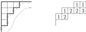
Figure 3. The Young diagram $\lambda(0100101011)$ and a semi-standard Young tableau of skew shape $\lambda(011011100)/\lambda(001011011)$.

There are skew shaped Young diagrams which play an important role in the context of Wieland drift: a skew shape is said to be a horizontal strip (resp. a vertical strip) if each of its columns (resp. rows) contains at most one cell. Consider two words $\omega$ and $\sigma$ satisfying $|\omega|_{1}=|\sigma|_{1}$, $|\omega|_{0}=|\sigma|_{0}$ and $\omega\leq\sigma$. Then the skew shape $\lambda(\sigma)/\lambda(\omega)$ is a horizontal strip (resp. a vertical strip) if and only if for each $j\in\{1,\dots,|\omega|_{1}\}$ (resp. for each $j\in\{1,2,\dots,|\omega|_{0}\}$) the following holds: If $\omega_{i}$ is the $j$-th one (resp. zero) in $\omega$ then $\sigma_{i-1}$ or $\sigma_{i}$ (resp. $\sigma_{i}$ or $\sigma_{i+1}$) is the $j$-th one (resp. zero) in $\sigma$. In the following, if the skew shaped Young diagram $\lambda(\sigma)/\lambda(\omega)$ is a horizontal strip (resp. a vertical strip) it will be written $\omega\stackrel{{\scriptstyle\mathrm{h}}}{{\longrightarrow}}\sigma$ (resp. $\omega\stackrel{{\scriptstyle\mathrm{v}}}{{\longrightarrow}}\sigma$).

Semi-standard Young tableaux of skew shape $\lambda(\sigma)/\lambda(\omega)$ with entries $1,2,\dots,m$ are in bijection with sequences of Young diagrams

$$\lambda(\omega)=\lambda(\tau^{0})\subseteq\lambda(\tau^{1})\subseteq\cdots\subseteq\lambda(\tau^{m-1})\subseteq\lambda(\tau^{m})=\lambda(\sigma),$$

such that $\tau^{i-1}\stackrel{{\scriptstyle\mathrm{h}}}{{\longrightarrow}}\tau^{i}$ for each $1\leq i\leq m$. To be more precise, the horizontal strip $\lambda(\tau^{i})/\lambda(\tau^{i-1})$ gives the cells of the semi-standard Young tableau of skew-shape $\lambda(\sigma)/\lambda(\omega)$ that have entry $i$ for $1\leq i\leq m$. For instance, the semi-standard Young tableau of skew shape $\lambda(011011100)/\lambda(001011011)$ in Figure 3 corresponds to the sequence

$$\lambda(001011011)\subseteq\lambda(010101110)\subseteq\lambda(011011010)\subseteq\lambda(011011100).$$

2.2. Triangular fully packed loop configurations

To give the definition of triangular fully packed loop configurations the following graph is needed:

Definition 2.1 (The graph $G^{N}$).

Let $N$ be a positive integer. The graph $G^{N}$ is defined as the induced subgraph of the square grid made up of $N$ consecutive centered rows of $3,5,\dots,2N+1$ vertices from top to bottom together with $2N+1$ vertical external edges incident to the $2N+1$ bottom vertices.

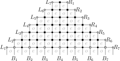
Figure 4. The graph $G^{7}$.

In Figure 4, the graph $G^{7}$ is depicted. From now on, the vertices of $G^{N}$ are partitioned into odd and even vertices in a chessboard manner where by convention the leftmost vertex of the top row of $G^{N}$ is odd. In the figures, odd vertices are represented by circles and even vertices by squares. There are vertices of $G^{N}$ that play a special role: let $\mathcal{L}^{N}=\{L_{1},L_{2},\dots,L_{N}\}$ (resp. $\mathcal{R}^{N}=\{R_{1},R_{2},\dots,R_{N}\}$) be the set made up of the vertices which are leftmost (resp. rightmost) in each of the $N$ rows of $G^{N}$ and let $\mathcal{B}^{N}=\{B_{1},B_{2},\dots,B_{N}\}$ be the set made up of the even vertices of the bottom row of $G^{N}$. The vertices are numbered from left to right. Furthermore, the $N(N+1)$ unit squares of $G^{N}$ including external unit squares that have three surrounding edges only are said to be the cells of $G^{N}$. They are partitioned into odd and even cells in a chessboard manner where by convention the top left cell of $G^{N}$ is odd.

Definition 2.2 (Triangular fully packed loop configuration).

Let $N$ be a positive integer. A triangular fully packed loop configuration (TFPL) of size $N$ is a subgraph $f$ of $G^{N}$ such that:

1. Precisely those external edges that are incident to a vertex in $\mathcal{B}^{N}$ are occupied by $f$.

2. The $2N$ vertices in $\mathcal{L}^{N}\cup\mathcal{R}^{N}$ have degree 0 or 1.

3. All other vertices of $G^{N}$ have degree 2.

4. A path in $f$ neither connects two vertices of $\mathcal{L}^{N}$ nor two vertices of $\mathcal{R}^{N}$.

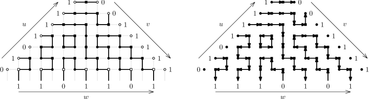
Figure 5. A TFPL of size $7$ and an oriented TFPL of size $7$.

An example of a TFPL is given in Figure 5. A cell of $f$ is a cell of $G^{N}$ together with those of its surrounding edges that are occupied by $f$. To each TFPL of size $N$ is assigned a triple of words of length $N$.

Definition 2.3.

Let $f$ be a TFPL of size $N$. The triple $(u,v;w)$ of words of length $N$ is assigned to $f$ as follows:

1. For $i=1,\dots,N$ set $u_{i}=1$ if the vertex $L_{i}\in\mathcal{L}^{N}$ has degree $1$ and $u_{i}=0$ otherwise.

2. For $i=1,\dots,N$ set $v_{i}=0$ if the vertex $R_{i}\in\mathcal{R}^{N}$ has degree $1$ and $v_{i}=1$ otherwise.

3. For $i=1,\dots,N$ set $w_{i}=1$ if in $f$ the vertex $B_{i}\in\mathcal{B}^{N}$ is connected with a vertex in $\mathcal{L}^{N}$ or with a vertex $B_{h}$ for an $h<i$ and $w_{i}=0$ otherwise.

The triple $(u,v;w)$ is said to be the boundary of $f$. Furthermore, the set of TFPLs with boundary $(u,v;w)$ is denoted by $T_{u,v}^{w}$ and its cardinality by $t_{u,v}^{w}$.

For example, the triple $(0101111,0011111;1101101)$ is the boundary of the TFPL depicted in Figure 5. The definitions of both a TFPL and its boundary contain global conditions. Those can be omitted when adding an orientation to each edge of a TFPL.

Definition 2.4 (Oriented triangular fully packed loop configuration).

An oriented TFPL of size $N$ is a TFPL of size $N$ together with an orientation of its edges such that the edges attached to $\mathcal{L}^{N}$ are outgoing, the edges attached to $\mathcal{R}^{N}$ are incoming and all other vertices of $G^{N}$ are incident to an incoming and an outgoing edge.

In Figure 5, an example of an oriented TFPL of size $7$ is given. In the underlying TFPL of an oriented TFPL condition (4) can be omitted because the required orientations of the edges attached to a vertex of the left or right boundary prevent paths from returning to the respective boundary.

Definition 2.5.

An oriented TFPL $f$ has boundary $(u,v;w)$ if the following hold:

1. If the vertex $L_{i}\in\mathcal{L}^{N}$ has out-degree $1$ then $u_{i}=1$. Otherwise, $u_{i}=0$.

2. If the vertex $R_{i}\in\mathcal{R}^{N}$ has in-degree $1$ then $v_{i}=0$. Otherwise, $v_{i}=1$.

3. If the external edge attached to the vertex $B_{i}\in\mathcal{B}^{N}$ is outgoing then $w_{i}=1$. Otherwise, $w_{i}=0$.

While $u$ and $v$ coincide with the respective boundary word in the underlying ordinary TFPL this is not the case for $w$. Instead of the connectivity of the paths $w$ encodes the local orientation of the edges. Only in the case when in an oriented TFPL all paths between two vertices $B_{i}$ and $B_{j}$ of $\mathcal{B}^{N}$ are oriented from $B_{i}$ to $B_{j}$ if $i<j$ the boundary word $w$ coincides with the respective boundary word of the underlying TFPL. Hence, the canonical orientation of a TFPL is defined as the orientation of the edges of the TFPL that satisfies the conditions in Definition 2.4 and in addition that each path between two vertices $B_{i},B_{j}\in\mathcal{B}^{N}$ is oriented from $B_{i}$ to $B_{j}$ if $i<j$ and that all closed paths are oriented clockwise.

A triple $(u,v;w)$ that is the boundary of an ordinary or an oriented TFPL has to fulfill the following conditions: $|u|_{0}=|v|_{0}=|w|_{0}$, $u\leq w$, $v\leq w$ and $d(w)-d(u)-d(v)\geq 0$. These conditions were proved in [4, 11, 5]. The last condition gives rise to the following definition:

Definition 2.6 ([5]).

Let $u,v,w$ be words of length $N$. Then the excess of $u,v,w$ is defined as

$$exc(u,v;w)=d(w)-d(u)-d(v).$$

If $exc(u,v;w)=k$ then both an ordinary and an oriented TFPL with boundary $(u,v;w)$ are said to be of excess $k$.

In [5], the following interpretation of the excess of $u,v,w$ in terms of numbers of occurrences of certain local configurations in an oriented TFPL with boundary $(u,v;w)$ is proved:

Proposition 2.7 ([5, Theorem 4.3]).

Let $f$ be an oriented TFPL with boundary $(u,v;w)$. Then

(2.1) $$\textnormal{exc}(u,v;w)=\vbox{\hbox{\includegraphics[width=4.77051pt]{Expose5}}}+\vbox{\hbox{\includegraphics[width=4.77051pt]{Expose6}}}+\vbox{\hbox{\includegraphics[width=35.7755pt]{Expose7}}}+\vbox{\hbox{\includegraphics[width=35.7755pt]{Expose8}}}+\vbox{\hbox{\includegraphics[width=20.273pt]{Expose9}}}+\vbox{\hbox{\includegraphics[width=20.273pt]{Expose10}}}+\vbox{\hbox{\includegraphics[width=20.273pt]{Expose11}}}+\vbox{\hbox{\includegraphics[width=20.273pt]{Expose12}}}$$

where by , , etc. the numbers of occurrences of the local configurations , , etc. in $f$ are denoted.

2.3. Blue-red path tangles

In this subsection an alternative representation of oriented TFPLs is introduced, namely blue-red path tangles. They came up in [5] and are crucial for the proofs given in this article. Throughout this subsection, let $u,v,w$ be words of length $N$ such that $|u|_{0}=|v|_{0}=|w|_{0}=N_{0}$, $|u|_{1}=|v|_{1}=|w|_{1}=N_{1}$, $u\leq w$, $v\leq w$ and $d(u)+d(v)\leq d(w)$.

A blue-red path tangle consists of an $N_{0}$-tuple of non-intersecting blue lattice paths and an $N_{1}$-tuple of non-intersecting red lattice paths. The blue lattice paths use steps $(-1,1)$, $(-1,-1)$ and $(-2,0)$, whereas the red lattice paths use steps $(1,1)$, $(1,-1)$ and $(2,0)$. Furthermore, neither a blue nor a red lattice path goes below the $x$-axis. The $k$-th blue lattice path of an $N_{0}$-tuple of non-intersecting blue lattice paths starts in a certain fixed vertex $D_{k}$ and ends in a certain fixed vertex $E_{k}$. The definitions of the vertices $D_{k}$ and $E_{k}$ solely depend on the positions of the $k$-th zeroes in $w$ and $u$ and are omitted here. Instead, the vertices $D_{1},\dots,D_{N_{0}}$ and $E_{1},\dots,E_{N_{0}}$ are indicated with an example in Figure 6. In the following, the set of $N_{0}$-tuples of non-intersecting blue lattice paths $(P_{1},P_{2},\dots,P_{N_{0}})$ where $P_{k}$ is a path from $D_{k}$ to $E_{k}$ is denoted by $\mathcal{P}(u,w)$. On the other hand, the $\ell$-th red path of an $N_{1}$-tuple of non-intersecting red lattice paths starts in a certain fixed vertex $D^{\prime}_{\ell}$ and ends in a certain fixed vertex $E^{\prime}_{\ell}$. The definitions of the vertices $D^{\prime}_{\ell}$ and $E^{\prime}_{\ell}$ solely depend on the positions of the $\ell$-th ones in $w$ and $v$ and are omitted here. Instead, $D^{\prime}_{\ell}$ and $E^{\prime}_{\ell}$ are indicated with and example in Figure 6. In the following, the set of $N_{1}$-tuples of non-intersecting red paths $(P^{\prime}_{1},P_{2}^{\prime},\dots,P_{N_{1}}^{\prime})$ where $P^{\prime}_{\ell}$ is a path from $D_{\ell}^{\prime}$ to $E_{\ell}^{\prime}$ is denoted by $\mathcal{P}^{\prime}(v,w)$.

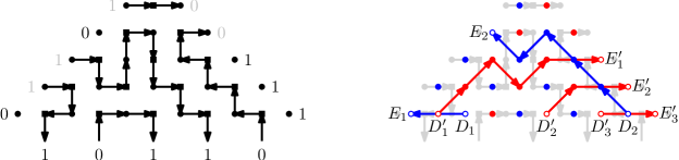
Figure 6. An oriented TFPL with boundary $(01101,00111;10110)$ and its corresponding blue-red path tangle with boundary $(01101,00111;10110)$.

Proposition 2.8 ([5, Theorem 4.1]).

The set of oriented TFPLs with boundary $(u,v;w)$ is in bijection with the set of pairs $(B,R)\in\mathcal{P}(u,w)\times\mathcal{P}^{\prime}(v,w)$ that satisfy the two following conditions:

1. No diagonal step of $R$ can cross a diagonal step of $B$.

2. Each middle point of a horizontal step in $B$ (resp. $R$) is used by a step in $R$ (resp. $B$).

The set of such configurations is denoted by BlueRed$(u,v;w)$ and a configuration in BlueRed$(u,v;w)$ is said to be a blue-red path tangle with boundary $(u,v;w)$.

An example of an oriented TFPL and its corresponding blue-red path tangle is given in Figure 6.

Proof.

Here the bijection in [5] is repeated: let $f$ be an oriented TFPL of size $N$ and with boundary $(u,v;w)$. As a start blue vertices are inserted in the middle of each horizontal edge of $G^{N}$ which has an odd vertex to its left and red vertices are inserted in the middle of each horizontal edge of $G^{N}$ which has an even vertex to its left. Next, blue edges are inserted as indicated in the left part of Figure 7 and red edges are inserted as indicated in the right part of Figure 7.

Figure 7. From oriented TFPLs to blue-red path tangles.

Then the blue vertices together with the blue edges give rise to an $N_{0}$-tuple of non-intersecting paths $B=(P_{1},P_{2},\dots,P_{N_{0}})$ in $\mathcal{P}(u,w)$ and the red vertices together with the red edges give rise to an $N_{1}$-tuple of non-intersecting paths $R=(P^{\prime}_{1},P_{2}^{\prime},\dots,P_{N_{1}}^{\prime})$ in $\mathcal{P}^{\prime}(v,w)$. The fact that no diagonal step of $R$ crosses a diagonal step of $B$ is equivalent to that there is a unique orientation of each vertical edge in $f$. On the other hand, the fact that each middle point of a horizontal step in $B$ (resp. $R$) is used by a step in $R$ (resp. $B$) is equivalent to that there is a unique orientation of each horizontal edge in $f$. Thus, $(B,R)\in\textnormal{BlueRed}(u,v;w)$. ∎

3. Wieland drift

The starting point of this section is the definition of Wieland gyration for fully packed loop configurations (FPLs) as introduced in [12]. Wieland gyration is composed of local operations on all active cells of an FPL: the active cells of an FPL can be chosen to be either all its odd cells or all its even cells. Given an active cell $c$ of an FPL two cases have to be distinguished, namely whether $c$ contains precisely two edges of the FPL on opposite sides or not. If this is the case, Wieland gyration $\operatorname{W}$ leaves $c$ invariant. Otherwise, the effect of $\operatorname{W}$ on $c$ is that edges and non-edges of the FPL are exchanged. In Figure 8, the action of $\operatorname{W}$ on an active cell is illustrated.

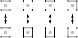
Figure 8. Up to rotation, the action of $\operatorname{W}$ on an active internal cell of an FPL.

Also left- and right-Wieland drift will be composed of local operations on all active cells of a TFPL. Similar to FPLs active cells of a TFPL are either chosen to be all its odd or all its even cells. Choosing all odd cells as active cells will lead to what will be defined as left-Wieland drift, whereas choosing all even cells as active cells will lead to what will be defined as right-Wieland drift. In the figures, the active cells of a TFPL will be indicated by gray circles.

Definition 3.1 (Left-Wieland drift).

Let $f$ be a TFPL with left boundary word $u$ and let $u^{-}$ be a word satisfying $u^{-}\stackrel{{\scriptstyle\mathrm{h}}}{{\longrightarrow}}u$. The image of $f$ under left-Wieland drift with respect to $u^{-}$ is determined as follows:

1. Insert a vertex $L^{\prime}_{i}$ to the left of $L_{i}$ for $1\leq i\leq N$. Then run through the occurrences of ones in $u^{-}$: Let $\{i_{1}<i_{2}<\ldots<i_{N_{1}}\}=\{i|u^{-}_{i}=1\}$.

   1. If $u_{i_{j}}$ is the $j$-th one in $u$, add a horizontal edge between $L^{\prime}_{i_{j}}$ and $L_{i_{j}}$.

   2. If $u_{i_{j}-1}$ is the $j$-th one in $u$, add a vertical edge between $L^{\prime}_{i_{j}}$ and $L_{{i_{j}}-1}$.

2. Apply Wieland gyration to each odd cell of $f$.

3. Delete all vertices in $\mathcal{R}^{N}$ and their incident edges.

After shifting the whole construction one unit to the right, one obtains the desired image $\operatorname{WL}_{u^{-}}(f)$. In the case $u^{-}=u$, simply write $\operatorname{WL}(f)$ and say the image of $f$ under left-Wieland drift.

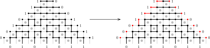
Figure 9. A TFPL and its image under left-Wieland drift with respect to $0001111$.

In Figure 9, an example for left-Wieland drift is given. The image of a TFPL with boundary $(u,v;w)$ under left-Wieland drift with respect to $u^{-}$ is again a TFPL and has boundary $(u^{-},v^{+};w)$, where $v^{+}$ is a word satisfying $v\stackrel{{\scriptstyle\mathrm{v}}}{{\longrightarrow}}v^{+}$, see [1, Proposition 2.2].

Right-Wieland drift depends on a word $v^{-}$ satisfying $v^{-}\stackrel{{\scriptstyle\mathrm{v}}}{{\longrightarrow}}v$ that encodes what happens along the right boundary of a TFPL with right boundary $v$ and is denoted by $\operatorname{WR}_{v^{-}}$ respectively $\operatorname{WR}$ if $v^{-}=v$. It is defined in an obvious way as the symmetric version of left-Wieland drift and it shall simply be illustrated with an example in Figure 10.

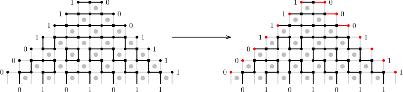
Figure 10. A TFPL and its image under right-Wieland drift with respect to $0001111$.

The image of a TFPL with boundary $(u,v;w)$ under right-Wieland drift with respect to $v^{-}$ is a TFPL with boundary $(u^{+},v^{-};w)$ where $u^{+}$ is a word satisfying $u\stackrel{{\scriptstyle\mathrm{h}}}{{\longrightarrow}}u^{+}$.

Given a TFPL with right boundary $v$ the effect of left-Wieland drift along the right boundary of the TFPL is inverted by right-Wieland drift with respect to $v$. On the other hand, given a TFPL with left boundary $u$ the effect of right-Wieland drift along the left boundary is inverted by left-Wieland drift with respect to $u$. Since Wieland gyration is an involution on each cell it follows:

Proposition 3.2 ([1, Theorem 2]).

1. Let $f$ be a TFPL with boundary $(u^{+},v;w)$ and $u$ be a word such that $u\stackrel{{\scriptstyle\mathrm{h}}}{{\longrightarrow}}u^{+}$. Then

   $$\operatorname{WR}_{v}(\operatorname{WL}_{u}(f))=f.$$

2. Let $f$ be a TFPL with boundary $(u,v^{+};w)$ and $v$ be a word such that $v\stackrel{{\scriptstyle\mathrm{v}}}{{\longrightarrow}}v^{+}$. Then

   $$\operatorname{WL}_{u}(\operatorname{WR}_{v}(f))=f.$$

By Proposition 3.2 a TFPL is invariant under left-Wieland drift if and only if it is invariant under right-Wieland drift. Hence, a TFPL is said to be stable if it is invariant under left-Wieland drift, whereas otherwise it is said to be instable. The set of stable TFPLs with boundary $(u,v;w)$ is denoted by $S_{u,v}^{w}$ and its cardinality by $s_{u,v}^{w}$. In [1] it is shown that stable TFPLs can be characterized as follows:

Proposition 3.3 ([1, Theorem 4]).

A TFPL is stable if and only if it contains no edge of the form . Such an edge is said to be a drifter.

Note that by Proposition 2.7 a TFPL of excess $k$ exhibits at most $k$ drifters.

Given a TFPL $f$ the sequence $(\operatorname{WL}^{m}(f))_{m\geq 0}$ is eventually periodic since there are only finitely many TFPLs of a fixed size. The length of its period is in fact always $1$.

Proposition 3.4 ([1, Theorem 3]).

Let $f$ be a TFPL of size $N$. Then $\operatorname{WL}^{2N-1}(f)$ is stable, so that the following holds for all $m\geq 2N-1$:

$$\operatorname{WL}^{m}(f)=\operatorname{WL}^{2N-1}(f).$$

The same holds for right-Wieland drift.

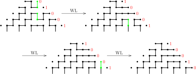
Figure 11. A TFPL and its images under left-Wieland drift.

In Figure 11 an example of a TFPL and its images under left-Wieland drift is given. There a stable TFPL is obtained after the third iteration of left-Wieland drift. From now on, for an instable TFPL $f$ denote by $L=L(f)$ the positive integer $L$ such that $\operatorname{WL}^{\ell}(f)$ is instable for each $0\leq\ell\leq L$ and $\operatorname{WL}^{L+1}(f)$ is stable and by $R=R(f)$ the positive integer such that $\operatorname{WR}^{r}(f)$ is instable for each $0\leq r\leq R$ and $\operatorname{WR}^{R+1}(f)$ is stable.

Definition 3.5 ($\operatorname{Path}(f)$, $\operatorname{Left}(f)$, $\operatorname{Right}(f)$).

Let $f$ be a TFPL. The path of $f$ – denoted by Path($f$) – is the sequence of all TFPLs that can be reached by an iterated application of left- respectively right-Wieland drift to $f$ that is

$$\operatorname{Path}(f)=\left(\operatorname{WR}^{R+1}(f),\dots,\operatorname{WR}(f),f,\operatorname{WL}(f),\dots,\operatorname{WL}^{L+1}(f)\right).$$

Furthermore, the stable TFPL $\operatorname{WR}^{R+1}(f)$ is denoted by $\operatorname{Right}(f)$ and the stable TFPL $\operatorname{WL}^{L+1}(f)$ by $\operatorname{Left}(f)$.

When $v^{\ell}$ denotes the right boundary of $\operatorname{WL}^{\ell}(f)$ for each $0\leq\ell\leq L+1$ and $\lambda^{\prime}$ denotes the conjugate of a Young diagram $\lambda$ then the sequence

(3.1) $$\lambda(v)^{\prime}=\lambda(v^{0})^{\prime}\subseteq\lambda(v^{1})^{\prime}\subseteq\cdots\subseteq\lambda(v^{L})^{\prime}\subseteq\lambda(v^{L+1})^{\prime}$$

gives rise to a semi-standard Young tableau of skew shape $\lambda(v^{L+1})/\lambda(v)^{\prime}$ with entries $1,2,\dots,L+1$. On the other hand, when $u^{r}$ denotes the left boundary of $\operatorname{WR}^{r}(f)$ for each $0\leq r\leq R+1$ then the sequence

(3.2) $$\lambda(u)=\lambda(u^{0})\subseteq\lambda(u^{1})\subseteq\cdots\subseteq\lambda(u^{R})\subseteq\lambda(u^{R+1}).$$

gives rise to a semi-standard Young tableau of skew shape $\lambda(u^{R+1})/\lambda(u)$.

It will be shown that for an instable TFPL $f$ with boundary $(u,v;w)$ of excess at most $2$ precisely one of the following cases applies:

1. the sequence in (3.1) corresponds to a semi-standard Young tableau in $G_{\lambda(v)^{\prime},\lambda(v^{+})^{\prime}}$;

2. the sequence in (3.2) corresponds to a semi-standard Young tableau in $G_{\lambda(u),\lambda(u^{+})}$;

3. neither the sequence in (3.1) corresponds to a semi-standard Young tableau in $G_{\lambda(v)^{\prime},\lambda(v^{+})^{\prime}}$ nor the sequence in (3.2) corresponds to a semi-standard Young tableau in $G_{\lambda(u),\lambda(u^{+})}$.

In the bijective proof of Theorem 1 an instable TFPL $f$ with boundary $(u,v;w)$ of excess at most $2$ will be associated with the triple consisting of the empty semi-standard Young tableau of skew shape $\lambda(u)/\lambda(u)$, the stable TFPL $\operatorname{Left}(f)$ and the semi-standard Young tableau corresponding to the sequence in (3.1) if the latter is an element of $G_{\lambda(v)^{\prime},\lambda(v^{+})^{\prime}}$. If the semi-standard Young tableau corresponding to the sequence in (3.2) is an element of $G_{\lambda(u),\lambda(u^{+})}$ then $f$ will be associated with the triple consisting of the semi-standard Young tableau in $G_{\lambda(u),\lambda(u^{R+1})}$ corresponding to the previous sequence, the stable TFPL $\operatorname{Right}(f)$ and the empty semi-standard Young tableau of skew shape $\lambda(v)^{\prime}/\lambda(v)^{\prime}$. Finally, if neither the sequence in (3.1) corresponds to a semi-standard Young tableau in $G_{\lambda(v)^{\prime},\lambda(v^{+})^{\prime}}$ nor the sequence in (3.2) corresponds to a semi-standard Young tableau in $G_{\lambda(u),\lambda(u^{+})}$ then to $f$ moves are applied which transform and ultimately turn it into a stable TFPL with boundary $(u^{+},v^{+};w)$ for a $u^{+}>u$ and a $v^{+}>v$. These moves will be extracted from the effect of Wieland drift on instable TFPLs of excess at most $2$. The triple which will be associated with $f$ then consists of this stable TFPL, a semi-standard Young tableau in $G_{\lambda(v)^{\prime},\lambda(v^{+})^{\prime}}$ and one in $G_{\lambda(u),\lambda(u^{+})}$.

In the next section, the effect of Wieland drift on instable TFPLs of excess at most $2$ is studied.

4. An alternative description of Wieland drift for TFPLs of excess at most 2

The main contribution of this section is a description of the effect of Wieland drift on TFPLs of excess at most $2$ as a composition of moves. In Figure 12, the moves which form the basis for that description are depicted. Recall that a TFPL of excess $k$ contains at most $k$ drifters.

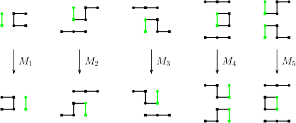
Figure 12. The moves performed by left-Wieland drift in an instable TFPL of excess at most $2$.

Proposition 4.1.

Let $f$ be an instable TFPL with boundary $(u,v;w)$ such that $\operatorname{exc}(u,v;w)\leq 2$. Furthermore, let $u^{-}$ be a word so that $u^{-}\stackrel{{\scriptstyle\mathrm{h}}}{{\longrightarrow}}u$. Then the image of $f$ under left-Wieland drift with respect to $u^{-}$ is determined as follows:

1. if $R_{i}$ in $\mathcal{R}^{N}$ is incident to a drifter delete that drifter and add a horizontal edge incident to $R_{i+1}$ for $i=1,2,\dots,N-1$; denote the so-obtained TFPL by $f^{\prime}$;

2. consider the columns of vertices of $G^{N}$ that contain a vertex, which is incident to a drifter in $f^{\prime}$: let $\mathcal{I}=\{\ 2\leq i\leq 2N:\,\,a\,\,vertex\,\,of\,\,the\,\,i-th\,\,column\,\ is\,\,incident\,\,to\,\,a\,\,drifter\,\,in\,\,f^{\prime}\}$, where the columns of $G^{N}$ are counted from left to right.

   1. If $\mathcal{I}=\{i<j\}$ apply a move in $\{M_{1},M_{2},M_{3}\}$ to the drifter incident to vertices of the $j$-th column and thereafter apply a move in $\{M_{1},M_{2},M_{3}\}$ to the drifter incident to vertices of the $i$-th column;

   2. If $\mathcal{I}=\{i\}$ perform a move in $\{M_{4},M_{5}\}$ or if this is not possible apply a move in $\{M_{1},M_{2},M_{3}\}$ to each of the drifters in $f^{\prime}$ in the following order (if there are two drifters in $f^{\prime}$): if the odd cell that contains the upper drifter is not of the form $\mathfrak{o}_{9}$ (see Figure 14) move the upper drifter first. Otherwise, move the lower drifter first.

3. run through the occurrences of one in $u^{-}$: let $\{i_{1}<i_{2}<\cdots<i_{N_{1}}\}=\{i:u_{i}^{-}=1\}$. If $u_{i_{j}-1}$ is the $j$-th one in $u$ delete the horizontal edge incident to $L_{i_{j}-1}$ and add a vertical edge incident to $L_{i_{j}}$ for $j=1,2,\dots,N_{1}$.

In Figure 13 a TFPL of excess $2$ with two drifters and its image under left-Wieland drift are depicted. The two drifters in the original TFPL have the same $x$-coordinate and the odd cell that contains the upper drifter is of the form $\mathfrak{o}_{9}$. Now, by left-Wieland drift the move $M_{1}$ is applied to the lower drifter before the move $M_{2}$ is applied to the other drifter. The rest of the TFPL is preserved.

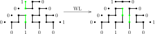
Figure 13. A TFPL of excess $2$ with two drifters and its image under left-Wieland drift.

In the proof of Proposition 4.1 the effect of left-Wieland drift will be checked cell by cell. From the set of cells that can occur in a TFPL of excess at most $2$ the following cells can be excluded:

Lemma 4.2.

In a TFPL of excess at most $2$, none of the following cells can occur:

Since the proofs in this section work by studying the cells of a TFPL it is convenient to fix notations for all the odd and even cells that can occur in a TFPL. In total, there are 16 different odd and 16 different even internal cells – that are cells which are not external – that can occur in a TFPL. By Lemma 4.2 fourteen of those odd and fourteen of those even internal cells that can occur in a TFPL of excess at most $2$. The odd respectively even cells that can occur in a TFPL of excess at most $2$ will be numbered by $1$ up to $14$ and are listed in Figure 14, whereas the two excluded odd respectively even internal cells will be numbered by $15$ and $16$ as indicated in Lemma 4.2.

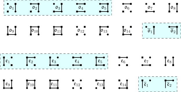
Figure 14. The cells of a TFPL of excess at most $2$ where the sets $\mathfrak{O}=\{\mathfrak{o}_{1},\mathfrak{o}_{2},\mathfrak{o}_{3},\mathfrak{o}_{4},\mathfrak{o}_{5},\overline{\mathfrak{o}}_{1},\overline{\mathfrak{o}}_{2}\}$ and $\mathfrak{E}=\{\mathfrak{e}_{1},\mathfrak{e}_{2},\mathfrak{e}_{3},\mathfrak{e}_{4},\mathfrak{e}_{5},\overline{\mathfrak{e}}_{1},\overline{\mathfrak{e}}_{2}\}$ are indicated.

Proof.

First, let $f$ be a TFPL that contains a cell $c$ that coincides with $\mathfrak{o}_{15}$. In $f$ together with its canonical orientation the oriented edges of $c$ then give rise to two configurations that are counted by the excess, see Proposition 2.7. Additionally, the right vertex of the horizontal edge of $c$ which is oriented from right to left either is adjacent to the vertex to its right or is incident to a drifter. Thus, the TFPL $f$ together with its canonical orientation contains at least three configurations that are counted by the excess. For the same reasons, a TFPL of excess at most $2$ cannot contain the third cell in the list.

Now, let $f$ be a TFPL that contains a cell $c$ that coincides with $\mathfrak{o}_{16}$. Then both the top and the bottom rightmost vertex of $c$ have to be incident to a drifter. Therefore, $f$ contains at least three drifters and therefore has to be of excess at least $3$. By the same argument, the fourth cell in the list cannot occur in a TFPL of excess at most $2$. ∎

In the following, to distinguish between the cells of a TFPL and the cells of its image under left-Wieland drift given a cell $c$ of $G^{N}$ it is written $c$ when it is referred to the cell $c$ of the TFPL and $c^{\prime}$ when it is referred to the cell $c$ of the image of the TFPL under left-Wieland drift. When the cells of a TFPL and of its image under left-Wieland drift are compared it has to be kept in mind that in the last step of left-Wieland drift the whole configuration is shifted one unit to the right. For that reason, for each odd cell $o$ of a TFPL and the even cell $e$ to the right of $o$ the following holds when disregarding the distinction between odd and even vertices:

$e^{\prime}=\operatorname{W}(o)$

The odd cells $\mathfrak{O}=\{\mathfrak{o}_{1},\mathfrak{o}_{2},\mathfrak{o}_{3},\mathfrak{o}_{4},\mathfrak{o}_{5},\overline{\mathfrak{o}}_{1},\overline{\mathfrak{o}}_{2}\}$ and the even cells $\mathfrak{E}=\{\mathfrak{e}_{1},\mathfrak{e}_{2},\mathfrak{e}_{3},\mathfrak{e}_{4},\mathfrak{e}_{5},\overline{\mathfrak{e}}_{1},\overline{\mathfrak{e}}_{2}\}$ play a special role in the context of Wieland drift.

Lemma 4.3 ([1]).

Let $f$ be a TFPL, $o$ an odd cell of $f$ and $e$ the even cell to the right of $o$. If no vertex of $o$ and $e$ is incident to a drifter, then

$$(o,e)\in\{(\mathfrak{o}_{1},\mathfrak{e}_{5}),(\mathfrak{o}_{2},\mathfrak{e}_{3}),(\mathfrak{o}_{3},\mathfrak{e}_{2}),(\mathfrak{o}_{4},\mathfrak{e}_{4}),(\mathfrak{o}_{5},\mathfrak{e}_{1}),(\overline{\mathfrak{o}}_{1},\overline{\mathfrak{e}}_{2}),(\overline{\mathfrak{o}}_{2},\overline{\mathfrak{e}}_{1})\}.$$

In particular, $e^{\prime}=e$ in that case.

To study the effect of left-Wieland drift on the whole TFPL it suffices to study its effect on the even cells of a TFPL. That is because edges of a TFPL that are not edges of an even cell have to be incident to a vertex in $\mathcal{L}^{N}$ and the effect of left-Wieland drift on these edges immediately follows from the definition of left-Wieland drift. To be more precise, in the image of a TFPL under left-Wieland drift all edges incident to a vertex in $\mathcal{L}^{N}$ have to be horizontal edges. By Lemma 4.3, to determine the effect of left-Wieland drift on a TFPL it suffices to determine its effect on the one hand on all even cells of the TFPL whereof a vertex is incident to a drifter and on the other hand on all even cells where the odd cells to their left contain a drifter.

Now, given a drifter $\mathfrak{d}$ in an instable TFPL there are at most three even cells whereof a vertex is incident to $\mathfrak{d}$ and there is at most one even cell such that the odd cell to its left contains $\mathfrak{d}$. In Figure 15, these four even cells together with the odd cells to their left are depicted. Note that all four such even cells exist if and only if $\mathfrak{d}$ is not incident to a vertex in $\mathcal{L}^{N}\cup\mathcal{R}^{N}$. From now on, these even cells and the odd cells to their left are denoted as indicated in Figure 15.

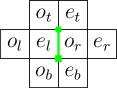
Figure 15. The even cells whereof a vertex is incident to a fixed drifter and the even cell such that the odd cell to its left contains the fixed drifter.

Given a drifter in a TFPL of excess at most $2$ the effect of left-Wieland drift on the cell $e_{t}$, $e_{l}$ respectively $e_{b}$ can be uniformly described as long as $o_{t}$, $o_{l}$ respectively $o_{b}$ does not contain a drifter and is not in $\{\mathfrak{o}_{6},\mathfrak{o}_{7},\mathfrak{o}_{12}\}$:

Lemma 4.4.

Let $f$ be an instable TFPL of excess at most $2$, $o$ an odd cell of $f$ and $e$ the even cell to the right of $o$. If $o$ does not contain a drifter, a vertex of $e$ is incident to a drifter and $o\notin\{\mathfrak{o}_{6}$, $\mathfrak{o}_{7}$, $\mathfrak{o}_{12}\}$, then $e^{\prime}$ and $e$ coincide with the following sole exceptions:

1. if in $e$ there is a drifter, then in $e^{\prime}$ there is none,

2. if the top left vertex of $e$ is incident to a drifter, then there is no horizontal edge between the two top vertices of $e$ but there is one between the two top vertices of $e^{\prime}$,

3. if the bottom left vertex of $e$ is incident to a drifter, then there is no horizontal edge between the two bottom vertices of $e$ but there is one between the two bottom vertices of $e^{\prime}$.

Proof.

If $o$ and $e$ are external cells such that a vertex of $e$ is incident to a drifter, then $o=\overline{\mathfrak{o}}_{1}$, $e=\overline{\mathfrak{e}}_{1}$ and $e^{\prime}=\overline{\mathfrak{e}}_{2}$. In that case, $e^{\prime}$ and $e$ coincide with the sole exception that there is no horizontal edge between the two top vertices of $e$ whereas there is one between the two top vertices of $e^{\prime}$. Suppose that $o$ and $e$ are internal cells such that $o$ does not contain a drifter, a vertex of $e$ is incident to a drifter and $o$ is not in $\{\mathfrak{o}_{6}$, $\mathfrak{o}_{7}$, $\mathfrak{o}_{12}\}$. Then $(o,e)$ can only occur as part of one of the following pairs:

Now, $e^{\prime}=\mathfrak{e}_{5}$ if $o=\mathfrak{o}_{1}$, $e^{\prime}=\mathfrak{e}_{3}$ if $o=\mathfrak{o}_{2}$, $e^{\prime}=\mathfrak{e}_{2}$ if $o=\mathfrak{o}_{3}$, $e^{\prime}=\mathfrak{e}_{4}$ if $o=\mathfrak{o}_{4}$ and $e^{\prime}=\mathfrak{e}_{1}$ if $o=\mathfrak{o}_{5}$. It can easily be checked that in any case $e^{\prime}$ and $e$ satisfy the assertions. ∎

In the following, separate proofs for each case in Proposition 4.1 will be given.

Proof of Proposition 4.1(1).

Let $f$ be an instable TFPL of excess at most $2$ that contains precisely one drifter $\mathfrak{d}$. First, the case when $\mathfrak{d}$ is incident to a vertex $R_{i}$ in $\mathcal{R}^{N}$ is considered. In that case the cells $o_{l}$, $e_{l}$, $o_{b}$ and $e_{b}$ exist. Furthermore, both $o_{l}$ and $o_{b}$ do not contain a drifter and are not in $\{\mathfrak{o}_{6},\mathfrak{o}_{7},\mathfrak{o}_{12}\}$ because in $f$ there is only one drifter. Thus, by Lemma 4.4 on the one hand $e^{\prime}_{l}$ and $e_{l}$ coincide with the sole exception that in $e^{\prime}_{l}$ there is no drifter whereas in $e_{l}$ there is one and on the other hand $e^{\prime}_{b}$ and $e_{b}$ coincide with the sole exception that in $e^{\prime}_{b}$ the two top vertices are adjacent whereas in $e_{b}$ they are not. By Lemma 4.3 the effect of left-Wieland drift on $f$ is that the drifter incident to $R_{i}$ is replaced by a horizontal edge incident to $R_{i+1}$ while the rest of $f$ is preserved.

It remains to consider the case when $\mathfrak{d}$ is not incident to a vertex in $\mathcal{R}^{N}$. In that case the cells $o_{r}$, $e_{r}$, $o_{b}$ and $e_{b}$ of $f$ have to exist. Since $f$ contains precisely one drifter $o_{r}\in\{\mathfrak{o}_{8},\mathfrak{o}_{9},\mathfrak{o}_{10},\mathfrak{o}_{11}\}$ by Lemma 4.2. It will be proceeded by treating each of the four possible cases for $o_{r}$ separately.

First, the case when $o_{r}=\mathfrak{o}_{8}$ is regarded. In that case, $e_{r}=\mathfrak{e}_{5}$ because $f$ contains precisely one drifter. Furthermore, $\operatorname{W}(\mathfrak{o}_{8})=\mathfrak{o}_{8}$ and therefore $e^{\prime}_{r}=\mathfrak{e}_{8}$. On the other hand, $e^{\prime}_{b}$ and $e_{b}$ coincide with the sole exception that the two top vertices in $e^{\prime}_{b}$ are adjacent whereas in $e_{b}$ they are not by Lemma 4.4. If the cells $o_{t}$, $e_{t}$, $o_{l}$ and $e_{l}$ exist, then both $o_{t}$ and $o_{l}$ cannot be in $\{\mathfrak{o}_{6},\mathfrak{o}_{7},\mathfrak{o}_{12}\}$ and for that reason $e^{\prime}_{t}$ and $e_{t}$ coincide with the sole exception that the two bottom vertices in $e^{\prime}_{t}$ are adjacent whereas in $e_{t}$ they are not and $e^{\prime}_{l}$ and $e_{l}$ coincide with the sole exception that in $e^{\prime}_{l}$ there is no drifter whereas in $e_{l}$ there is one by Lemma 4.4. By Lemma 4.3, the effect of left-Wieland drift on $f$ is that the move $M_{1}$ is applied to $\mathfrak{d}$ while the rest of $f$ is preserved.

Next, the case when $o_{r}=\mathfrak{o}_{9}$ is considered. In that case, $e_{r}=\mathfrak{e}_{2}$, $o_{b}=\mathfrak{o}_{7}$ and $e_{b}=\mathfrak{e}_{4}$. Furthermore, $\operatorname{W}(\mathfrak{o}_{9})=\mathfrak{o}_{6}$ that is $e^{\prime}_{r}=\mathfrak{e}_{6}$ and $\operatorname{W}(\mathfrak{o}_{7})=\mathfrak{o}_{10}$ that is $e^{\prime}_{b}=\mathfrak{e}_{10}$. If the cells $o_{l}$, $e_{l}$, $o_{t}$ and $e_{t}$ exist, then neither $o_{t}$ nor $o_{l}$ is in $\{\mathfrak{o}_{6},\mathfrak{o}_{7},\mathfrak{o}_{12}\}$. By Lemma 4.4 and Lemma 4.3 the effect of left-Wieland drift on $f$ is that the move $M_{2}$ is applied to $\mathfrak{d}$ while the rest of $f$ is preserved.

Next, the case when $o_{r}=\mathfrak{o}_{10}$ is regarded. In that case, $o_{t}$, $e_{t}$, $o_{l}$ and $e_{l}$ exist. Furthermore, $e_{r}=\mathfrak{e}_{3}$, $o_{t}=\mathfrak{o}_{6}$ and $e_{t}=\mathfrak{e}_{4}$. Therefore, $e^{\prime}_{r}=\mathfrak{e}_{7}$ and $e^{\prime}_{t}=\mathfrak{e}_{9}$. Since neither $o_{b}$ nor $o_{l}$ is in $\{\mathfrak{o}_{6},\mathfrak{o}_{7},\mathfrak{o}_{12}\}$ by Lemma 4.4 and Lemma 4.3 the effect of left-Wieland drift on $f$ is that the move $M_{3}$ is applied to $\mathfrak{d}$ while the rest of $f$ is preserved.

Finally, the case when $o_{r}=\mathfrak{o}_{11}$ is checked. In that case $o_{t}$, $e_{t}$, $o_{l}$ and $e_{l}$ exist. Furthermore, $e_{r}=\mathfrak{e}_{1}$, $o_{b}=\mathfrak{o}_{7}$, $e_{b}=\mathfrak{e}_{4}$, $o_{l}=\mathfrak{o}_{5}$, $e_{l}=\mathfrak{e}_{8}$, $o_{t}=\mathfrak{o}_{6}$ and $e_{t}=\mathfrak{e}_{4}$. Therefore, $e^{\prime}_{r}=\mathfrak{e}_{12}$, $e^{\prime}_{b}=\mathfrak{e}_{10}$, $e^{\prime}_{l}=\mathfrak{e}_{1}$ and $e^{\prime}_{t}=\mathfrak{e}_{9}$. By Lemma 4.3 the effect of left-Wieland drift on $f$ is that the move $M_{4}$ is applied to $\mathfrak{d}$ while the rest of $f$ is preserved. ∎

Proof of Proposition 4.1(2a).

Let $f$ be a TFPL of excess $2$ that contains two drifters which are both incident to a vertex in $\mathcal{R}^{N}$. In the following, denote the two drifter in $f$ by $\mathfrak{d}$ and $\mathfrak{d}^{\ast}$ and let $R_{i}$ and $R_{i^{\ast}}$ be the vertices in $\mathcal{R}^{N}$ to which $\mathfrak{d}$ and $\mathfrak{d}^{\ast}$ are incident. The cells $o_{l}$, $e_{l}$, $o_{b}$ and $e_{b}$ and the cells $o_{l}^{\ast}$, $e_{l}^{\ast}$, $o_{b}^{\ast}$ and $e_{b}^{\ast}$ exist. Furthermore, none of the cells $o_{l}$, $o_{b}$, $o_{l}^{\ast}$ and $o_{b}^{\ast}$ contains a drifter or is of the form $\mathfrak{o}_{6}$, $\mathfrak{o}_{7}$ or $\mathfrak{o}_{12}$. Therefore, by Lemma 4.4 and Lemma 4.3 the effect of left-Wieland drift on $f$ is that both drifters are replaced by horizontal edges incident to $R_{i+1}$ and $R_{i^{\ast}+1}$ while the rest of $f$ remains unchanged. ∎

Proof of Proposition 4.1(2b).

Let $f$ be a TFPL of excess $2$ that contains two drifters $\mathfrak{d}$ and $\mathfrak{d}^{\ast}$ whereof $\mathfrak{d}$ is incident to a vertex $R_{i}$ in $\mathcal{R}^{N}$ and $\mathfrak{d}^{\ast}$ is not incident to a vertex in $\mathcal{R}^{N}$. Note that $f$ contains neither a cell of type $\mathfrak{o}_{11}$ nor of type $\mathfrak{e}_{11}$. That is because when adding the canonical orientation to $f$ such a cell would give rise to two local configurations that are counted by the excess which would imply that $f$ is of excess greater than $2$. As a start, suppose that no vertex of $o_{l}$ and $o_{b}$ is incident to $\mathfrak{d}^{\ast}$. In that case $e^{\prime}_{l}$ and $e_{l}$ coincide with the sole exception that in $e^{\prime}_{l}$ there is no drifter and $e^{\prime}_{b}$ and $e_{b}$ coincide with the sole exception that in $e^{\prime}_{b}$ the two top vertices are adjacent whereas in $e_{b}$ they are not by Lemma 4.4. On the other hand, since $\mathfrak{d}^{\ast}$ is not incident to a vertex in $\mathcal{R}^{N}$ the cells $o_{r}^{\ast}$, $e_{r}^{\ast}$, $o_{b}^{\ast}$ and $e_{b}^{\ast}$ exist. Futhermore, no vertex of $o_{r}^{\ast}$, $e_{r}^{\ast}$, $o_{b}^{\ast}$ and $e_{b}^{\ast}$ is incident to $\mathfrak{d}$. If the cells $o_{l}^{\ast}$, $e_{l}^{\ast}$, $o_{t}^{\ast}$ and $e_{t}^{\ast}$ exist then also no vertex of these cells is incident to $\mathfrak{d}$. For those reasons, by analogous arguments as in the proof of Proposition 4.1(1) the effect of left-Wieland drift on $f$ is that $\mathfrak{d}$ is replaced by a horizontal edge incident to $R_{i+1}$ before a unique move of $\{M_{1},M_{2},M_{3}\}$ is applied to $\mathfrak{d}^{\ast}$. The rest of $f$ is preserved by left-Wieland drift.

Now, if the bottom right vertex of $o_{b}$ is incident to $\mathfrak{d}^{\ast}$, then $o_{r}^{\ast}\in\{\mathfrak{o}_{8},\mathfrak{o}_{9},\mathfrak{o}_{10}\}$. If $o_{r}^{\ast}=\mathfrak{o}_{8}$, then $e_{r}^{\ast}=\mathfrak{e}_{5}$. Furthermore, $o_{l}$, $o_{b}$, $o_{l}^{\ast}$ and $o_{b}^{\ast}$ do not contain a drifter and are not in $\{\mathfrak{o}_{6},\mathfrak{o}_{7},\mathfrak{o}_{12}\}$. Thus, the effect of left-Wieland drift is that $\mathfrak{d}$ is replaced by a horizontal edge incident to $R_{i+1}$ before the move $M_{1}$ is applied to $\mathfrak{d}^{\ast}$ while the rest of $f$ is preserved. If $o_{r}^{\ast}=\mathfrak{o}_{9}$, then $e_{r}^{\ast}=\mathfrak{e}_{2}$, $o_{b}^{\ast}=\mathfrak{o}_{7}$ and $e_{b}^{\ast}=\mathfrak{e}_{4}$. Additionally, $o_{l}$, $o_{b}$ and $o_{l}$ do not contain a drifter and are not in $\{\mathfrak{o}_{6},\mathfrak{o}_{7},\mathfrak{o}_{12}\}$. Therefore, the effect of left-Wieland drift is that $\mathfrak{d}$ is replaced by a horizontal edge incident to $R_{i+1}$ before the move $M_{2}$ is applied to $\mathfrak{d}^{\ast}$ while the rest of $f$ is preserved. Finally, if $o_{r}^{\ast}=\mathfrak{o}_{10}$, then $e_{r}^{\ast}=\mathfrak{e}_{3}$, $o_{b}=\mathfrak{o}_{6}$ and $e_{b}=\mathfrak{e}_{7}$. Furthermore, $o_{l}$, $o_{l}^{\ast}$ and $o_{b}^{\ast}$ do not contain a drifter and are not in $\{\mathfrak{o}_{6},\mathfrak{o}_{7},\mathfrak{o}_{12}\}$. For those reasons, the effect of left-Wieland drift is that $\mathfrak{d}$ is replaced by a horizontal edge incident to $R_{i+1}$ before the move $M_{3}$ is applied to $\mathfrak{d}^{\ast}$ while the rest of $f$ is preserved.

Next, if $o_{l}$ contains $\mathfrak{d}^{\ast}$, then $o_{l}=\mathfrak{o}_{10}$, $e_{l}=\mathfrak{e}_{9}$, $o_{t}^{\ast}=\mathfrak{o}_{6}$, $e_{t}^{\ast}=\mathfrak{e}_{4}$, $o_{b}=\mathfrak{o}_{4}$, $e_{b}=\mathfrak{e}_{7}$ and $o_{b}^{\ast}\notin\{\mathfrak{o}_{6},\mathfrak{o}_{7},\mathfrak{o}_{12}\}$. Therefore, $e^{\prime}_{l}=\mathfrak{e}_{7}$, $e^{\prime}_{t}=\mathfrak{e}_{9}$, $e^{\prime}_{b}=\mathfrak{e}_{4}$ and by Lemma 4.4 the cells $e^{\ast\prime}_{b}$ and $e_{b}^{\ast}$ coincide with the sole exception that in $e^{\ast\prime}_{b}$ there is an edge between the two top vertices whereas in $e_{b}^{\ast}$ there is none. For those reasons, the effect of left-Wieland drift on $f$ is that $\mathfrak{d}$ is replaced by a horizontal edge incident to $R_{i+1}$ before the move $M_{3}$ is applied to $\mathfrak{d}^{\ast}$ while the rest of $f$ is preserved.

Finally, if $o_{b}$ contains $\mathfrak{d}^{\ast}$, then $o_{b}\in\{\mathfrak{o}_{8},\mathfrak{o}_{9}\}$. If $o_{b}=\mathfrak{o}_{8}$, then $e_{b}=\mathfrak{e}_{3}$. Furthermore, none of the cells $o_{l}$, $o_{l}^{\ast}$ and $o_{b}^{\ast}$ is in $\{\mathfrak{o}_{6},\mathfrak{o}_{7},\mathfrak{o}_{12}\}$. Thus, the effect of left-Wieland drift on $f$ is that $\mathfrak{d}$ is replaced by a horizontal edge incident to $R_{i+1}$ before the move $M_{1}$ is applied to $\mathfrak{d}^{\ast}$ while the rest of $f$ is preserved. On the other hand, if $o_{b}=\mathfrak{o}_{9}$, then $e_{b}=\mathfrak{e}_{1}$, $o_{b}^{\ast}=\mathfrak{o}_{7}$ and $e_{b}^{\ast}=\mathfrak{e}_{4}$. Additionally, $o_{l}$ and $o_{l}^{\ast}$ do not contain a drifter and are not in $\{\mathfrak{o}_{6},\mathfrak{o}_{7},\mathfrak{o}_{12}\}$. Therefore, the effect of left-Wieland drift on $f$ is that $\mathfrak{d}$ is replaced by a horizontal edge incident to $R_{i+1}$ before the move $M_{2}$ is applied to $\mathfrak{d}^{\ast}$ while the rest of $f$ is preserved. ∎

Proof of Proposition 4.1(2c).

Let $f$ be a TFPL of excess $2$ that contains two drifters whereof none is incident to a vertex in $\mathcal{R}^{N}$. In that case the cells $o_{r}$, $e_{r}$, $o_{b}$, $e_{b}$ and the cells $o_{r}^{\ast}$, $e_{r}^{\ast}$, $o_{b}^{\ast}$, $e_{b}^{\ast}$ exist. Furthermore, both $o_{r}$ and $o_{r}^{\ast}$ have to be in $\{\mathfrak{o}_{8},\mathfrak{o}_{9},\mathfrak{o}_{10},\mathfrak{o}_{13},\mathfrak{o}_{14}\}$. It is started with the case when no vertex of the cells $o_{r}$, $e_{r}$, $o_{b}$, $e_{b}$ is incident to $\mathfrak{d}^{\ast}$ and no vertex of the cells $o_{r}^{\ast}$, $e_{r}^{\ast}$, $o_{b}^{\ast}$, $e_{b}^{\ast}$ is incident to $\mathfrak{d}$. This implies that if the cells $o_{l}$, $e_{l}$, $o_{t}$ and $e_{t}$ exist then none of their vertices is incident to $\mathfrak{d}^{\ast}$ and if the cells $o_{l}^{\ast}$, $e_{l}^{\ast}$, $o_{t}^{\ast}$ and $e_{t}^{\ast}$ exist then none of their vertices is incident to $\mathfrak{d}$. Therefore, by the same arguments as in the proof of Proposition 4.1(1) the effect of left-Wieland drift on $f$ is that simultaneously to each of the two drifters $\mathfrak{d}$ and $\mathfrak{d}^{\ast}$ a unique move in $\{M_{1},M_{2},M_{3}\}$ is applied while the rest of $f$ is conserved. Since the moves can be performed simultaneously they can be performed in the order stated in Proposition 4.1(2).

It remains to study the case when a vertex of $o_{r}$, $e_{r}$, $o_{b}$ or $e_{b}$ is incident to $\mathfrak{d}^{\ast}$ or a vertex of $o_{r}^{\ast}$, $e_{r}^{\ast}$, $o_{b}^{\ast}$ or $e_{b}^{\ast}$ is incident to $\mathfrak{d}$. Hence, without loss of generality assume that a vertex of the cells $o_{r}$, $e_{r}$, $o_{b}$, $e_{b}$ that is not the top right vertex of $o_{r}$ is incident to the drifter $\mathfrak{d}^{\ast}$. Then $o_{r}$ does not equal $\mathfrak{o}_{14}$ and $o_{r}^{\ast}$ does not equal $\mathfrak{o}_{13}$.

As a start, the case when the bottom right vertex of $o_{b}$ is incident to $\mathfrak{d}^{\ast}$ is considered. In that case $\mathfrak{d}$ and $\mathfrak{d}^{\ast}$ have the same $x$-coordinate and $\mathfrak{d}$ has the larger $y$-coordinates than $\mathfrak{d}^{\ast}$. If the cells $o_{t}$, $e_{t}$, $o_{l}$ and $e_{l}$ exist then $o_{t}$ neither equals $\mathfrak{o}_{7}$ nor $\mathfrak{o}_{12}$. Furthermore, if $o_{t}=\mathfrak{o}_{6}$ then $e_{t}=\mathfrak{e}_{4}$, $o_{r}=\mathfrak{o}_{10}$ and $e_{r}=\mathfrak{e}_{3}$. Thus, $e^{\prime}_{t}=\mathfrak{e}_{9}$ and $e^{\prime}_{r}=\mathfrak{e}_{7}$. On the other hand, if $o_{t}$ does not equal $\mathfrak{o}_{6}$ then $e^{\prime}_{t}$ and $e_{t}$ coincide with the sole exception that in $e^{\prime}_{t}$ there is a horizontal edge between its two bottom vertices whereas in $e_{t}$ there is none by Lemma 4.4. Since neither $o_{l}$ nor $o_{l}^{\ast}$ equals $\mathfrak{o}_{6}$, $\mathfrak{o}_{7}$ or $\mathfrak{o}_{12}$ the cells $e^{\prime}_{l}$ and $e_{l}$ (resp. $e^{\ast\prime}_{l}$ and $e_{l}^{\ast}$) coincide with the sole exception that in $e^{\prime}_{l}$ (resp. $e^{\ast\prime}_{l}$) there is no drifter by Lemma 4.4. Finally, $o_{b}^{\ast}$ does neither equal $\mathfrak{o}_{6}$ nor $\mathfrak{o}_{12}$ and if it equals $\mathfrak{o}_{7}$ then $e_{b}^{\ast}=\mathfrak{e}_{4}$, $o_{r}^{\ast}=\mathfrak{o}_{9}$, $e_{r}^{\ast}=\mathfrak{e}_{2}$, $e^{\ast\prime}_{b}=\mathfrak{e}_{10}$ and $e^{\ast\prime}_{r}=\mathfrak{e}_{3}$.

By Lemma 4.3, it remains to study the cells $o_{r}$, $e_{r}$, $o_{b}$, $e_{b}$, $o_{r}^{\ast}$, $e_{r}^{\ast}$, $e_{r}^{\prime}$, $e_{b}^{\prime}$ and $e_{r}^{\ast\prime}$. A list of all possible configurations in the cells $o_{r}$, $e_{r}$, $o_{b}$, $e_{b}$, $o_{r}^{\ast}$, $e_{r}^{\ast}$, $e_{r}^{\prime}$, $e_{b}^{\prime}$ and $e_{r}^{\ast\prime}$ is given in Table 1.

$o_{r}$

$\mathfrak{o}_{8}$

$\mathfrak{o}_{8}$

$\mathfrak{o}_{8}$

$\mathfrak{o}_{8}$

$\mathfrak{o}_{8}$

$\mathfrak{o}_{9}$

$\mathfrak{o}_{9}$

$\mathfrak{o}_{9}$

$\mathfrak{o}_{10}$

$\mathfrak{o}_{10}$

$\mathfrak{o}_{10}$

$\mathfrak{o}_{10}$

$e_{r}$

$\mathfrak{e}_{5}$

$\mathfrak{e}_{5}$

$\mathfrak{e}_{5}$

$\mathfrak{e}_{5}$

$\mathfrak{e}_{5}$

$\mathfrak{e}_{2}$

$\mathfrak{e}_{2}$

$\mathfrak{e}_{2}$

$\mathfrak{e}_{3}$

$\mathfrak{e}_{3}$

$\mathfrak{e}_{3}$

$\mathfrak{e}_{3}$

$o_{r}^{\ast}$

$\mathfrak{o}_{8}$

$\mathfrak{o}_{8}$

$\mathfrak{o}_{9}$

$\mathfrak{o}_{9}$

$\mathfrak{o}_{10}$

$\mathfrak{o}_{8}$

$\mathfrak{o}_{9}$

$\mathfrak{o}_{10}$

$\mathfrak{o}_{8}$

$\mathfrak{o}_{8}$

$\mathfrak{o}_{9}$

$\mathfrak{o}_{10}$

$e_{r}^{\ast}$

$\mathfrak{e}_{5}$

$\mathfrak{e}_{5}$

$\mathfrak{e}_{2}$

$\mathfrak{e}_{2}$

$\mathfrak{e}_{3}$

$\mathfrak{e}_{5}$

$\mathfrak{e}_{2}$

$\mathfrak{e}_{3}$

$\mathfrak{e}_{5}$

$\mathfrak{e}_{5}$

$\mathfrak{e}_{2}$

$\mathfrak{e}_{3}$

$o_{b}$

$\mathfrak{o}_{1}$

$\mathfrak{o}_{4}$

$\mathfrak{o}_{1}$

$\mathfrak{o}_{4}$

$\mathfrak{o}_{6}$

$\mathfrak{o}_{7}$

$\mathfrak{o}_{7}$

$\mathfrak{o}_{12}$

$\mathfrak{o}_{1}$

$\mathfrak{o}_{4}$

$\mathfrak{o}_{4}$

$\mathfrak{o}_{6}$

$e_{b}$

$\mathfrak{e}_{1}$

$\mathfrak{e}_{12}$

$\mathfrak{e}_{1}$

$\mathfrak{e}_{12}$

$\mathfrak{e}_{7}$

$\mathfrak{e}_{6}$

$\mathfrak{e}_{6}$

$\mathfrak{e}_{4}$

$\mathfrak{e}_{1}$

$\mathfrak{e}_{12}$

$\mathfrak{e}_{12}$

$\mathfrak{e}_{7}$

$e^{\prime}_{r}$

$\mathfrak{e}_{8}$

$\mathfrak{e}_{8}$

$\mathfrak{e}_{8}$

$\mathfrak{e}_{8}$

$\mathfrak{e}_{8}$

$\mathfrak{e}_{6}$

$\mathfrak{e}_{6}$

$\mathfrak{e}_{6}$

$\mathfrak{e}_{7}$

$\mathfrak{e}_{7}$

$\mathfrak{e}_{7}$

$\mathfrak{e}_{7}$

$e^{\ast\prime}_{r}$

$\mathfrak{e}_{8}$

$\mathfrak{e}_{8}$

$\mathfrak{e}_{6}$

$\mathfrak{e}_{6}$

$\mathfrak{e}_{7}$

$\mathfrak{e}_{8}$

$\mathfrak{e}_{6}$

$\mathfrak{e}_{7}$

$\mathfrak{e}_{8}$

$\mathfrak{e}_{8}$

$\mathfrak{e}_{6}$

$\mathfrak{e}_{7}$

$e^{\prime}_{b}$

$\mathfrak{e}_{15}$

$\mathfrak{e}_{4}$

$\mathfrak{e}_{15}$

$\mathfrak{e}_{4}$

$\mathfrak{e}_{9}$

$\mathfrak{e}_{10}$

$\mathfrak{e}_{10}$

$\mathfrak{e}_{11}$

$\mathfrak{e}_{15}$

$\mathfrak{e}_{4}$

$\mathfrak{e}_{4}$

$\mathfrak{e}_{9}$

Table 1. The cells $o_{r},e_{r},o_{r}^{\ast},e_{r}^{\ast},o_{b}$ and $e_{b}$ of $f$ and the cells $e^{\prime}_{r},e^{\ast\prime}_{r}$ and $e^{\prime}_{b}$ of $\operatorname{WL}(f)$ in the case when $\mathfrak{d}^{\ast}$ is incident to the bottom right vertex of $o_{b}$ in $f$.

In summary, left-Wieland drift has the following effect:

• The move $M_{5}$ is applied if $o_{r}=\mathfrak{o}_{9}$ and $o_{r}^{\ast}=\mathfrak{o}_{10}$.

• The move $M_{1}$/$M_{2}$ is applied to $\mathfrak{d}^{\ast}$ before the move $M_{2}$ is applied to $\mathfrak{d}$ if $o_{r}=\mathfrak{o}_{9}$ and $o_{r}^{\ast}=\mathfrak{o}_{8}/\mathfrak{o}_{9}$.

• The move $M_{1}$ is applied to $\mathfrak{d}$ before the move $M_{1}$/$M_{2}$/$M_{3}$ is applied to $\mathfrak{d}^{\ast}$ if $o_{r}=\mathfrak{o}_{8}$ and $o_{r}^{\ast}=\mathfrak{o}_{8}/\mathfrak{o}_{9}/\mathfrak{o}_{10}$.

• The move $M_{3}$ is applied to $\mathfrak{d}$ before the move $M_{1}$/$M_{2}$/$M_{3}$ is applied to $\mathfrak{d}^{\ast}$ if $o_{r}=\mathfrak{o}_{10}$ and $o_{r}^{\ast}=\mathfrak{o}_{8}/\mathfrak{o}_{9}/\mathfrak{o}_{10}$.

In all cases the rest of $f$ is preserved by left-Wieland drift.

Next, the case when the drifter $\mathfrak{d}^{\ast}$ is contained in $e_{r}$ is studied. In that case the $x$-coordinate of $\mathfrak{d}^{\ast}$ is larger than the one of $\mathfrak{d}$. Note that $(o_{r},e_{r})\in\{(\mathfrak{o}_{9},\mathfrak{e}_{10}),(\mathfrak{o}_{10},\mathfrak{e}_{9})\}$ since $f$ contains neither of the cells $\mathfrak{o}_{11}$ and $\mathfrak{e}_{11}$. Now, if $o_{r}=\mathfrak{o}_{9}$ then $o_{b}=\mathfrak{o}_{7}$, $e_{b}=\mathfrak{e}_{4}$, $o_{t}^{\ast}=\mathfrak{o}_{4}$, $e_{t}^{\ast}=\mathfrak{e}_{6}$ and $(o_{r}^{\ast},e_{r}^{\ast})\in\{(\mathfrak{o}_{8},\mathfrak{e}_{5}),(\mathfrak{o}_{9},\mathfrak{e}_{2})\}$. Furthermore, if $o_{r}^{\ast}=\mathfrak{o}_{9}$ then $o_{b}^{\ast}=\mathfrak{o}_{7}$ and $e_{b}^{\ast}=\mathfrak{e}_{4}$. Thus, $e^{\prime}_{r}=\mathfrak{e}_{6}$, $e^{\prime}_{b}=\mathfrak{e}_{10}$, $e^{\ast\prime}_{t}=\mathfrak{e}_{4}$ and if $o_{r}^{\ast}=\mathfrak{o}_{9}$ then $e^{\ast\prime}_{r}=\mathfrak{e}_{6}$ and $e^{\ast\prime}_{b}=\mathfrak{e}_{10}$. On the other hand, if $o_{r}=\mathfrak{o}_{10}$ then $o_{t}=\mathfrak{o}_{6}$, $e_{t}=\mathfrak{e}_{4}$, $o_{b}^{\ast}=\mathfrak{o}_{4}$, $e_{b}^{\ast}=\mathfrak{e}_{7}$ and $(o_{r}^{\ast},e_{r}^{\ast})\in\{(\mathfrak{o}_{8},\mathfrak{e}_{5}),(\mathfrak{o}_{10},\mathfrak{e}_{3})\}$. Furthermore, if $o_{r}^{\ast}=\mathfrak{o}_{10}$ then $o_{t}^{\ast}=\mathfrak{o}_{6}$ and $e_{t}^{\ast}=\mathfrak{e}_{4}$. Thus, $e^{\prime}_{r}=\mathfrak{e}_{7}$, $e^{\prime}_{t}=\mathfrak{e}_{9}$ and $e^{\ast\prime}_{b}=\mathfrak{e}_{4}$ and if $o_{r}^{\ast}=\mathfrak{o}_{10}$ then $e^{\ast\prime}_{r}=\mathfrak{e}_{7}$ and $e^{\ast\prime}_{t}=\mathfrak{e}_{9}$. By Lemma 4.3 and Lemma 4.4 the effect of left-Wieland drift is the following:

• The move $M_{1}$/$M_{2}$ is applied to $\mathfrak{d}^{\ast}$ before the move $M_{2}$ is applied to $\mathfrak{d}$ if $o_{r}=\mathfrak{o}_{9}$ and $o_{r}^{\ast}=\mathfrak{o}_{8}/\mathfrak{o}_{9}$.

• The move $M_{1}$/$M_{3}$ is applied to $\mathfrak{d}^{\ast}$ before the move $M_{3}$ is applied to $\mathfrak{d}$ if $o_{r}=\mathfrak{o}_{10}$ and $o_{r}^{\ast}=\mathfrak{o}_{8}/\mathfrak{o}_{10}$.

In both cases the rest of $f$ is preserved by left-Wieland drift.

Next, the case when $\mathfrak{d}^{\ast}$ is contained in $e_{b}$ is regarded. In that case the $x$-coordinate of $\mathfrak{d}^{\ast}$ is larger than the one of $\mathfrak{d}$. The cells $o_{l}$ and $o_{b}$ are both not contained in $\{\mathfrak{o}_{6},\mathfrak{o}_{7},\mathfrak{o}_{12}\}$. For instance, it is not possible that $o_{b}$ equals $\mathfrak{o}_{7}$ because then $e_{b}$ would have to equal $e_{15}$ or the bottom right vertex of $o_{b}$ would be incident to a drifter. As a start, if $o_{t}$ exists then it cannot be in $\{\mathfrak{o}_{7},\mathfrak{o}_{12}\}$. Furthermore, if $o_{t}=\mathfrak{o}_{6}$ then $e_{t}=\mathfrak{e}_{4}$, $o_{r}=\mathfrak{o}_{10}$, $e_{r}=\mathfrak{e}_{3}$, $e_{t}^{\prime}=\mathfrak{e}_{9}$ and $e_{r}^{\prime}=\mathfrak{e}_{7}$. On the other hand, $o_{b}^{\ast}$ cannot be in $\{\mathfrak{o}_{6},\mathfrak{o}_{12}\}$. Furthermore, if $o_{b}^{\ast}=\mathfrak{o}_{7}$ then $e_{b}^{\ast}=\mathfrak{e}_{4}$, $o_{r}^{\ast}=\mathfrak{o}_{9}$, $e_{r}^{\ast}=\mathfrak{e}_{2}$, $e_{b}^{\ast\prime}=\mathfrak{e}_{10}$ and $e_{r}^{\ast\prime}=\mathfrak{e}_{6}$. To determine the effect of left-Wieland drift on $f$ it remains to study the cells $o_{r}^{\ast}$, $e_{r}^{\ast}$, $o_{r}$, $e_{r}$, $e_{r}^{\ast\prime}$ and $e_{r}^{\prime}$. In Table 3 all possible configurations in these cells are listed.

$o_{r}^{\ast}$	$\mathfrak{o}_{8}$	$\mathfrak{o}_{8}$	$\mathfrak{o}_{9}$	$\mathfrak{o}_{9}$	$\mathfrak{o}_{10}$
$e_{r}^{\ast}$	$\mathfrak{e}_{5}$	$\mathfrak{e}_{5}$	$\mathfrak{e}_{2}$	$\mathfrak{e}_{2}$	$\mathfrak{e}_{3}$
$o_{r}$	$\mathfrak{o}_{8}$	$\mathfrak{o}_{10}$	$\mathfrak{o}_{8}$	$\mathfrak{o}_{10}$	$\mathfrak{o}_{13}$
$e_{r}$	$\mathfrak{e}_{2}$	$\mathfrak{e}_{1}$	$\mathfrak{e}_{2}$	$\mathfrak{e}_{1}$	$\mathfrak{e}_{4}$
$e_{r}^{\ast\prime}$	$\mathfrak{e}_{8}$	$\mathfrak{e}_{8}$	$\mathfrak{e}_{6}$	$\mathfrak{e}_{6}$	$\mathfrak{e}_{7}$
$e_{r}^{\prime}$	$\mathfrak{e}_{8}$	$\mathfrak{e}_{7}$	$\mathfrak{e}_{8}$	$\mathfrak{e}_{7}$	$\mathfrak{e}_{14}$

Table 2. The cells $o_{r}^{\ast}$, $e_{r}^{\ast}$, $o_{r}$ and $e_{r}$ of $f$ and the cells $e_{r}^{\ast\prime}$ and $e^{\prime}_{r}$ of $\operatorname{WL}(f)$ in the case when $\mathfrak{d}^{\ast}$ is contained in $e_{b}$.

In summary, the effect of left-Wieland drift on $f$ is the following:

• The move $M_{1}$ is applied to $\mathfrak{d}^{\ast}$ before the move $M_{1}$/$M_{3}$ is applied to $\mathfrak{d}$ if $o_{r}^{\ast}=\mathfrak{o}_{8}$ and $o_{r}=\mathfrak{o}_{8}/\mathfrak{o}_{10}$.

• The move $M_{2}$ is applied to $\mathfrak{d}^{\ast}$ before the move $M_{1}$/$M_{3}$ is applied to $\mathfrak{d}$ if $o_{r}^{\ast}=\mathfrak{o}_{9}$ and $o_{r}=\mathfrak{o}_{8}/\mathfrak{o}_{10}$.

• The move $M_{3}$ is applied to $\mathfrak{d}^{\ast}$ before it also is applied to $\mathfrak{d}$ if $o_{r}^{\ast}=\mathfrak{o}_{10}$ and $o_{r}=\mathfrak{o}_{13}$.

In all cases the rest of $f$ is preserved by left-Wieland drift.

The last case that is to be considered is the case when $\mathfrak{d}^{\ast}$ is contained in $o_{b}$. In that case the $x$-coordinate of $\mathfrak{d}$ is larger than the one of $\mathfrak{d}^{\ast}$. Furthermore, the cells $o_{l}$ and $o_{l}^{\ast}$ are not contained in $\{\mathfrak{o}_{6},\mathfrak{o}_{7},\mathfrak{o}_{1}2\}$, if $o_{t}$ exists then it cannot be in $\{\mathfrak{o}_{7},\mathfrak{o}_{12}\}$ and $o_{b}^{\ast}$ cannot be in $\{\mathfrak{o}_{6},\mathfrak{o}_{12}\}$. On the other hand, if $o_{t}=\mathfrak{o}_{6}$ then $e_{t}=\mathfrak{e}_{4}$, $o_{r}=\mathfrak{o}_{10}$, $e_{r}=\mathfrak{e}_{3}$, $e_{t}^{\prime}=\mathfrak{e}_{9}$ and $e_{r}^{\prime}=\mathfrak{e}_{7}$ and if $o_{b}^{\ast}=\mathfrak{o}_{7}$ then $e_{b}^{\ast}=\mathfrak{e}_{4}$, $o_{r}^{\ast}=\mathfrak{o}_{9}$, $e_{r}^{\ast}=\mathfrak{e}_{2}$, $e_{b}^{\ast\prime}=\mathfrak{e}_{10}$ and $e_{r}^{\ast\prime}=\mathfrak{e}_{6}$. To determine the effect of left-Wieland drift on $f$ it remains to study the cells $o_{r}^{\ast}$, $e_{r}^{\ast}$, $o_{r}$, $e_{r}$, $e_{r}^{\ast\prime}$ and $e_{r}^{\prime}$. In Table 3 all possible configurations in these cells are listed.

$o_{r}$	$\mathfrak{o}_{8}$	$\mathfrak{o}_{8}$	$\mathfrak{o}_{9}$	$\mathfrak{o}_{10}$	$\mathfrak{o}_{10}$
$e_{r}$	$\mathfrak{e}_{5}$	$\mathfrak{e}_{5}$	$\mathfrak{e}_{2}$	$\mathfrak{e}_{3}$	$\mathfrak{e}_{3}$
$o_{b}$	$\mathfrak{o}_{8}$	$\mathfrak{o}_{9}$	$\mathfrak{o}_{14}$	$\mathfrak{o}_{8}$	$\mathfrak{o}_{9}$
$e_{b}$	$\mathfrak{e}_{3}$	$\mathfrak{e}_{1}$	$\mathfrak{e}_{4}$	$\mathfrak{e}_{3}$	$\mathfrak{e}_{1}$
$e^{\prime}_{r}$	$\mathfrak{e}_{8}$	$\mathfrak{e}_{8}$	$\mathfrak{e}_{6}$	$\mathfrak{e}_{7}$	$\mathfrak{e}_{7}$
$e^{\prime}_{b}$	$\mathfrak{e}_{8}$	$\mathfrak{e}_{6}$	$\mathfrak{e}_{3}$	$\mathfrak{e}_{8}$	$\mathfrak{e}_{6}$

Table 3. The cells $o_{r}$, $e_{r}$, $o_{b}$ and $e_{b}$ of $f$ and the cells $e^{\prime}_{r}$ and $e^{\prime}_{b}$ of $\operatorname{WL}(f)$ in the case when $\mathfrak{d}^{\ast}$ is contained in $o_{b}$.

By Lemma 4.3 and Lemma 4.4 the effect of left-Wieland drift on $f$ is the following:

• The move $M_{1}$ is applied to $\mathfrak{d}$ before the move $M_{1}$/$M_{2}$ is applied to $\mathfrak{d}^{\ast}$ if $o_{r}=\mathfrak{o}_{8}$ and $o_{b}=\mathfrak{o}_{8}/\mathfrak{o}_{9}$.

• The move $M_{2}$ is first applied to $\mathfrak{d}$ and then to $\mathfrak{d}^{\ast}$ if $o_{r}=\mathfrak{o}_{9}$ and $o_{b}=\mathfrak{o}_{14}$.

• The move $M_{3}$ is applied to $\mathfrak{d}$ before the move $M_{1}$/$M_{2}$ is applied to $\mathfrak{d}^{\ast}$ if $o_{r}=\mathfrak{o}_{10}$ and $o_{b}=\mathfrak{o}_{8}/\mathfrak{o}_{9}$.

∎

The description of the effect of right-Wieland drift on an instable TFPL of excess at most $2$ follows from the description of the effect of left-Wieland drift on an instable TFPL of excess at most $2$ by vertical symmetry.

Proposition 4.5.

Let $f$ be an instable TFPL with boundary $(u,v;w)$ such that $\operatorname{exc}(u,v;w)\leq 2$. Furthermore, let $v^{-}$ be a word so that $v^{-}\stackrel{{\scriptstyle\mathrm{v}}}{{\longrightarrow}}v$. Then the image of $f$ under right-Wieland drift with respect to $v^{-}$ is determined as follows:

1. if $L_{i}$ in $\mathcal{L}^{N}$ is incident to a drifter delete that drifter and add a horizontal edge incident to $L_{i-1}$ for $i=2,3,\dots,N$; denote the so-obtained TFPL by $f^{\prime}$;

2. consider the columns of vertices of $G^{N}$ that contain a vertex, which is incident to a drifter in $f^{\prime}$: let $\mathcal{I}=\{\ 2\leq i\leq 2N:\,\,a\,\,vertex\,\,of\,\,the\,\,i-th\,\,column\,\ is\,\,incident\,\,to\,\,a\,\,drifter\,\,in\,\,f^{\prime}\}$, where the columns of $G^{N}$ are counted from left to right.

   1. If $\mathcal{I}=\{i<j\}$ apply a move in $\{M_{1}^{-1},M_{2}^{-1},M_{3}^{-1}\}$ to the drifter incident to vertices of the $i$-th column and thereafter apply a move in $\{M_{1}^{-1},M_{2}^{-1},M_{3}^{-1}\}$ to the drifter incident to vertices of the $j$-th column;

   2. If $\mathcal{I}=\{i\}$ perform a move in $\{M_{4}^{-1},M_{5}^{-1}\}$ or if this is not possible apply a move in $\{M_{1}^{-1},M_{2}^{-1},M_{3}^{-1}\}$ to each of the drifters in $f^{\prime}$ in the following order (if there are two drifters in $f^{\prime}$): if the even cell that contains the lower drifter is not of the form $\mathfrak{o}_{10}$ (see Figure 14) move the lower drifter first. Otherwise, move the upper drifter first.

3. run through the occurrences of zero in $v^{-}$: let $\{i_{1}<i_{2}<\cdots<i_{N_{0}}\}=\{i:v_{i}^{-}=0\}$. If $v_{i_{j}+1}$ is the $j$-th zero in $v$ delete the horizontal edge incident to $R_{i_{j}+1}$ and add a vertical edge incident to $R_{i_{j}}$ for $j=1,2,\dots,N_{0}$.

5. The path of a drifter under Wieland drift for TFPLs of excess at most $2$

The focus of this section is on how many iterations of left-Wieland drift (resp. right-Wieland drift) are needed to move a drifter in an instable TFPL of excess at most $2$ to the right (resp. left) boundary. The results of the previous section facilitate the study of the effect of Wieland drift on a drifter in an instable TFPL of excess at most $2$. When looking at the moves that describe the effect of Wieland drift on instable TFPLs of excess at most $2$ one immediately sees that in the preimage of the move $M_{4}$ there is one drifter whereas in its image there two and that in the preimage of the move $M_{5}$ there are two drifters whereas in its image there is one. Thus, in order to pursue a drifter one has to decide which drifter to pursue after applying the move $M_{4}^{-1}$ resp. $M_{5}$. Hence, fix a drifter in the image of the move $M_{5}^{-1}$ that is identified with the drifter in the preimage and fix a drifter in the image of the move $M_{4}$ that is identified with the drifter in the preimage. For all other moves, identify the drifter in the image with the drifter in the preimage.

Given an instable TFPL $f$ of excess at most $2$ and a drifter $\mathfrak{d}$ in $f$ there exists a unique non-negative integer $L(\mathfrak{d})$ so that $\mathfrak{d}$ is incident to a vertex in $\mathcal{L}^{N}$ in $\operatorname{WL}^{L(\mathfrak{d})}(f)$ and $\mathfrak{d}$ is contained in $\operatorname{WL}^{\ell}(f)$ for each $0\leq\ell\leq L(\mathfrak{d})$ by Proposition 4.1. On the other hand, there exists a unique non-negative integer $R(\mathfrak{d})$ so that $\mathfrak{d}$ is incident to a vertex in $\mathcal{R}^{N}$ in $\operatorname{WR}^{R(\mathfrak{d})}(f)$ and $\mathfrak{d}$ is contained in $\operatorname{WR}^{r}(f)$ for each $0\leq r\leq R(\mathfrak{d})$ by Proposition 4.5. The main result of this section will be an expression for the sum $L(\mathfrak{d})+R(\mathfrak{d})$ in terms of boundary words and will be stated in Corollary 5.4.

Definition 5.1 ($\operatorname{Path}(\mathfrak{d}),\operatorname{Left}(\mathfrak{d}),\operatorname{Right}(\mathfrak{d}),\operatorname{HeightL}(\mathfrak{d}),\operatorname{HeightR}(\mathfrak{d})$).

Let $f$ be an instable TFPL of excess at most $2$ and $\mathfrak{d}$ be a drifter in $f$. The path of $\mathfrak{d}$ – denoted by $\operatorname{Path}(\mathfrak{d})$ – is defined as the sequence of all instable TFPLs that contain $\mathfrak{d}$ and can be reached by an iterated application of left- or right-Wieland drift to $f$. That is

$$\operatorname{Path}(\mathfrak{d})=\left(\operatorname{WR}^{R(\mathfrak{d})}(f),\dots,\operatorname{WR}(f),f,\operatorname{WL}(f),\dots,\operatorname{WL}^{L(\mathfrak{d})}(f)\right).$$

Furthermore, $\operatorname{WR}^{R(\mathfrak{d})}(f)$ is denoted by $\operatorname{Right}(\mathfrak{d})$ and $\operatorname{WL}^{L(\mathfrak{d})}(f)$ is denoted by $\operatorname{Left}(\mathfrak{d})$. The unique positive integer $h$ with $\mathfrak{d}$ incident to $L_{h+1}$ in $\operatorname{Right}(\mathfrak{d})$ is denoted by $\operatorname{HeigthR}(\mathfrak{d})$ and the unique positive integer $h^{\prime}$ with $\mathfrak{d}$ incident to $R_{N-h^{\prime}}$ in $\operatorname{Left}(\mathfrak{d})$ is denoted by $\operatorname{HeightL}(\mathfrak{d})$.

By definition it holds $|\operatorname{Path}(\mathfrak{d})|=L(\mathfrak{d})+R(\mathfrak{d})+1$. For $i=1,2,3,4,5$ set

$$\#M_{i}(\mathfrak{d}) =|\{0\leq r\leq R(\mathfrak{d})-1:\text{ by $\operatorname{WR}$ the move $M_{i}^{-1}$ is applied to $\mathfrak{d}$ in $\operatorname{WR}^{r}(f)$}\}|$$

$$+|\{0\leq\ell\leq L(\mathfrak{d})-1:\text{ by $\operatorname{WL}$ the move $M_{i}$ is applied to $\mathfrak{d}$ in $\operatorname{WL}^{\ell}(f)$}\}|.$$

Thus, $|\operatorname{Path}(\mathfrak{d})|=\#M_{1}(\mathfrak{d})+\#M_{2}(\mathfrak{d})+\#M_{3}(\mathfrak{d})+\#M_{4}(\mathfrak{d})+\#M_{5}(\mathfrak{d})+1$ and in summary

$$L(\mathfrak{d})+R(\mathfrak{d})=\#M_{1}(\mathfrak{d})+\#M_{2}(\mathfrak{d})+\#M_{3}(\mathfrak{d})+\#M_{4}(\mathfrak{d})+\#M_{5}(\mathfrak{d}).$$

Definition 5.2 ($R_{i}(u^{R(\mathfrak{d})})$, $L_{i}(v^{L(\mathfrak{d})})$).

Let $f$ be an instable TFPL with boundary $(u,v;w)$ of excess at most $2$ and $\mathfrak{d}$ a drifter in $f$. When $u^{R(\mathfrak{d})}$ denotes the left boundary of $\operatorname{WR}^{R(\mathfrak{d})}(f)$ and $v^{L(\mathfrak{d})}$ denotes the right boundary of $\operatorname{WL}^{L(\mathfrak{d})}(f)$ then define $R_{i}(u^{R(\mathfrak{d})})$ as the number of occurrences of $i$ among the last $(N-1-\operatorname{HeightR}(\mathfrak{d}))$ letters of $u^{R(\mathfrak{d})}$ and $L_{i}(v^{L(\mathfrak{d})})$ as the number of occurrences of $i$ among the first $(N-1-\operatorname{HeightL}(\mathfrak{d}))$ letters of $v^{L(\mathfrak{d})}$ for $i=0,1$.

Proposition 5.3.

Let $f$ be an instable TFPL with boundary $(u,v;w)$ where $exc(u,v;w)\leq 2$, $\mathfrak{d}$ a drifter in $f$ and the notations as above. Then

$$\#M_{1}(\mathfrak{d})+\#M_{2}(\mathfrak{d})+\#M_{3}(\mathfrak{d})+\#M_{4}(\mathfrak{d})+\#M_{5}(\mathfrak{d})=R_{1}(u^{R(\mathfrak{d})})+L_{0}(v^{L(\mathfrak{d})})+1.$$

The proof of Proposition 5.3 will be the content of the rest of this section. The crucial idea is to regard TFPLs together with their canonical orientation. Before starting with the proof a crucial corollary of Proposition 5.3 is stated.

Corollary 5.4.

Let $f$ be an instable TFPL with boundary $(u,v;w)$ where $exc(u,v;w)\leq 2$, $\mathfrak{d}$ a drifter in $f$ and the notations as above. Then

(5.1) $$L(\mathfrak{d})+R(\mathfrak{d})=R_{1}(u^{R(\mathfrak{d})})+L_{0}(v^{L(\mathfrak{d})})+1.$$

In Figure 16 an instable TFPL of excess $2$ and the path of one of its drifters which shall in the following be denoted by $\mathfrak{d}$ are depicted. The drifter $\mathfrak{d}$ satisfies $R(\mathfrak{d})=2$, $\operatorname{HeightR}(\mathfrak{d})=1$, $u^{R(\mathfrak{d})}=01101$, $R_{1}(u^{R(\mathfrak{d})})=2$, $L(\mathfrak{d})=2$, $\operatorname{HeightL}(\mathfrak{d})=2$, $v^{L(\mathfrak{d})}=01011$ and $L_{0}(v^{L(\mathfrak{d})})=1$.

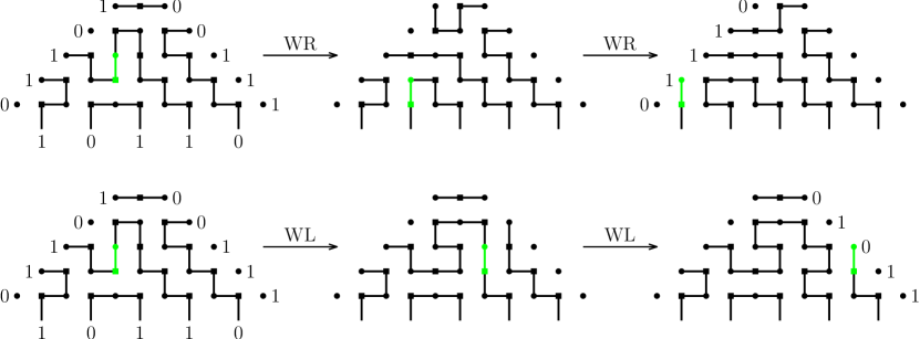
Figure 16. A TFPL with boundary $(01101,00111;10110)$ and the path of the drifter that is indicated in green.

The following lemma are immediate consequences of Proposition 2.7, Proposition 4.1 and Proposition 4.5 and describe the effect of Wieland drift on canonically oriented TFPLs of excess at most $2$. The moves that form the basis for this description derive from the moves in Figure 12 and are depicted in Figure 17. In particular, the moves $\overrightarrow{M}_{1,1}$, $\overrightarrow{M}_{1,2}$, $\overrightarrow{M}_{1,3}$, $\overrightarrow{M}_{1,4}$, $\overrightarrow{M}_{2,1}$ and $\overrightarrow{M}_{3,1}$ coincide with the moves $BB$, $BR$, $RR$, $RB$, $B$ and $R$ respectively invented in [5] for blue-red path tangles corresponding to instable oriented TFPLs of excess $1$.

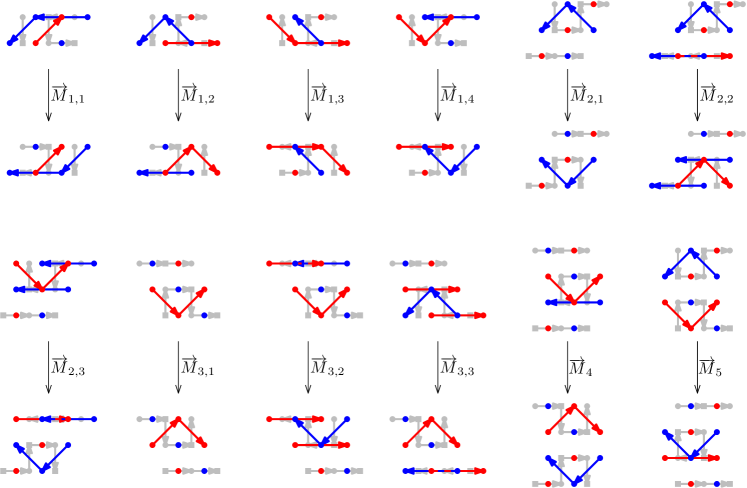
Figure 17. The moves describing the effect of Wieland drift on canonically oriented TFPLs of excess at most $2$. In addition, the moves are indicated in terms of blue-red path tangles.

Lemma 5.5.

Let $u,v,w$ be words of length $N$ such that $exc(u,v;w)\leq 2$ and $f$ an instable TFPL with boundary $(u,v;w)$ where not all drifters are incident to a vertex in $\mathcal{R}^{N}$. When $\overrightarrow{f}$ denotes $f$ together with the canonical orientation of its edges, then the effect of left-Wieland drift on $f$ translates into the following effect on $\overrightarrow{f}$:

1. If in $\overrightarrow{f}$ there is precisely one drifter then by left-Wieland drift a unique move in$\{\overrightarrow{M}_{1,1},\overrightarrow{M}_{1,2},\overrightarrow{M}_{1,3},\overrightarrow{M}_{1,4},\overrightarrow{M}_{2,1},\overrightarrow{M}_{2,2},\overrightarrow{M}_{2,3},\overrightarrow{M}_{3,1},\overrightarrow{M}_{3,2},\overrightarrow{M}_{3,3},\overrightarrow{M}_{4}\}$ is performed while the rest of $\overrightarrow{f}$ remains unchanged.

2. If in $\overrightarrow{f}$ there are two drifters and none of those drifters is incident to a vertex in $\mathcal{R}^{N}$ then by left-Wieland drift either $\overrightarrow{M}_{5}$ is performed or to each drifter a unique move in $\{\overrightarrow{M}_{1,1},\overrightarrow{M}_{1,2},\overrightarrow{M}_{1,3},\overrightarrow{M}_{1,4},\overrightarrow{M}_{2,1},\overrightarrow{M}_{3,1}\}$ is applied in the same order as in Proposition 4.1. The rest of $\overrightarrow{f}$ remains unchanged.

3. Finally, if in $\overrightarrow{f}$ there are two drifters whereof one is incident to a vertex in $\mathcal{R}^{N}$ then by left-Wieland drift the drifter incident to a vertex $R_{i}$ in $\mathcal{R}^{N}$ is replaced by a horizontal edge incident to $R_{i+1}$ before to the remaining drifter a unique move in $\{\overrightarrow{M}_{1,1},\overrightarrow{M}_{1,2},\overrightarrow{M}_{1,3},\overrightarrow{M}_{1,4},\overrightarrow{M}_{2,1},\overrightarrow{M}_{3,1}\}$ is applied. The rest of $\overrightarrow{f}$ remains unchanged by left-Wieland drift.

Lemma 5.6.

Let $u,v,w$ be words of length $N$ such that $exc(u,v;w)\leq 2$ and $f$ an instable TFPL with boundary $(u,v;w)$ where not all drifters are incident to a vertex in $\mathcal{L}^{N}$. Then the effect of right-Wieland drift on $f$ translates into the following effect on $\overrightarrow{f}$:

1. If in $\overrightarrow{f}$ there is precisely one drifter then by right-Wieland drift a unique move in $\{\overrightarrow{M}^{-1}_{1,1},\overrightarrow{M}^{-1}_{1,2},\overrightarrow{M}^{-1}_{1,3},\overrightarrow{M}^{-1}_{1,4},\overrightarrow{M}^{-1}_{2,1},\overrightarrow{M}^{-1}_{2,2},\overrightarrow{M}^{-1}_{2,3},\overrightarrow{M}^{-1}_{3,1},\overrightarrow{M}^{-1}_{3,2},\overrightarrow{M}^{-1}_{3,3},\overrightarrow{M}^{-1}_{5}\}$ is performed while the rest of $\overrightarrow{f}$ remains unchanged.

2. If in $\overrightarrow{f}$ there are two drifters and none of those drifters is incident to a vertex in $\mathcal{L}^{N}$ then by right-Wieland drift either $\overrightarrow{M}^{-1}_{4}$ is performed or to each drifter in $\overrightarrow{f}$ a unique move in $\{\overrightarrow{M}^{-1}_{1,1},\overrightarrow{M}^{-1}_{1,2},\overrightarrow{M}^{-1}_{1,3},\overrightarrow{M}^{-1}_{1,4},\overrightarrow{M}^{-1}_{2,1},\overrightarrow{M}^{-1}_{3,1}\}$ is applied in the same order as in Proposition 4.5. The rest of $\overrightarrow{f}$ remains unchanged.

3. Finally, if in $\overrightarrow{f}$ there are two drifters whereof one is incident to a vertex in $\mathcal{L}^{N}$ then by right-Wieland drift the drifter incident to a vertex $L_{j}$ in $\mathcal{L}^{N}$ is replaced by a horizontal edge incident to $L_{j-1}$ before a unique move in $\{\overrightarrow{M}^{-1}_{1,1},\overrightarrow{M}^{-1}_{1,2},\overrightarrow{M}^{-1}_{1,3},\overrightarrow{M}^{-1}_{1,4},\overrightarrow{M}^{-1}_{2,1},\overrightarrow{M}^{-1}_{3,1}\}$ is applied to the remaining drifter. The rest of $\overrightarrow{f}$ remains unchanged by right-Wieland drift.

In the following, for $(i,j)=(1,1),(1,2),(1,3),(1,4),(2,1),(2,2),(2,3),(3,1),(3,2),(3,3)$ set

$$\#\overrightarrow{M}_{i,j}(\mathfrak{d}) =|\{0\leq r\leq R(\mathfrak{d})-1:\text{ by $\operatorname{WR}$ the move $\overrightarrow{M}_{i,j}^{-1}$ is applied to $\mathfrak{d}$ in $\operatorname{WR}^{r}(\overrightarrow{f})$}\}|$$

$$+|\{0\leq\ell\leq L(\mathfrak{d})-1:\text{ by $\operatorname{WL}$ the move $\overrightarrow{M}_{i,j}$ is applied to $\mathfrak{d}$ in $\operatorname{WL}^{\ell}(\overrightarrow{f})$}\}|.$$

For the moves $\overrightarrow{M}_{4}^{-1}$ and $\overrightarrow{M}_{5}$ it has to be distinguished which of the two drifters in the respective image is identified with the one in the preimage. Hence, for $i=4,5$ set

$$\#\overrightarrow{M}_{i} =|\{0\leq r\leq R(\mathfrak{d})-1:\text{ by $\operatorname{WR}$ the move $\overrightarrow{M}_{i}^{-1}$ is applied to $\mathfrak{d}$ in $\operatorname{WR}^{r}(\overrightarrow{f})$}\}|$$

$$+|\{0\leq\ell\leq L(\mathfrak{d})-1:\text{ by $\operatorname{WL}$ the move $\overrightarrow{M}_{i}$ is applied to $\mathfrak{d}$ in $\operatorname{WL}^{\ell}(\overrightarrow{f})$}\}|.$$

and indicate by a $t$ or $b$ whether in the respective image the top or the bottom drifter is identified with the drifter in the respective preimage. In that way, one obtains the notation $\#\overrightarrow{M}_{i}^{b}$ respectively $\#\overrightarrow{M}_{i}^{t}$ for $i=4,5$.

Lemma 5.7.

Let $f$ be an instable TFPL with boundary $(u,v;w)$ where $exc(u,v;w)\leq 2$ and $\mathfrak{d}$ a drifter in $f$. When $\overrightarrow{f}$ denotes $f$ together with the canonical orientation of its edges, then the following hold:

1. $\sum\limits_{i=1}^{4}\#\overrightarrow{M}_{1,i}(\mathfrak{d})+\sum\limits_{j=1}^{3}\#\overrightarrow{M}_{3,j}(\mathfrak{d})+\#\overrightarrow{M}_{4}^{t}(\mathfrak{d})+\#\overrightarrow{M}_{5}^{b}(\mathfrak{d})=N-\operatorname{HeightR}(\mathfrak{d})$,

2. $\sum\limits_{i=1}^{4}\#\overrightarrow{M}_{1,i}(\mathfrak{d})+\sum\limits_{j=1}^{3}\#\overrightarrow{M}_{2,j}(\mathfrak{d})+\#\overrightarrow{M}_{4}^{b}(\mathfrak{d})+\#\overrightarrow{M}_{5}^{t}(\mathfrak{d})=N-\operatorname{HeightL}(\mathfrak{d})$,

3. $\#\overrightarrow{M}_{1,1}(\mathfrak{d})+\#\overrightarrow{M}_{1,4}(\mathfrak{d})+\#\overrightarrow{M}_{2,3}(\mathfrak{d})-\#\overrightarrow{M}_{3,3}(\mathfrak{d})+\#\overrightarrow{M}_{4}^{b}(\mathfrak{d})=L_{1}(v^{L(\mathfrak{d})})$,

4. $\#\overrightarrow{M}_{1,2}(\mathfrak{d})+\#\overrightarrow{M}_{1,3}(\mathfrak{d})-\#\overrightarrow{M}_{2,3}(\mathfrak{d})+\#\overrightarrow{M}_{3,3}(\mathfrak{d})-\#\overrightarrow{M}_{4}^{b}(\mathfrak{d})=R_{0}(u^{R(\mathfrak{d})})+1$.

The identities in Lemma 5.7 generalize the identities of Proposition 6.11 and of Proposition 6.12 in [5] for $\#BB$, $\#BR$, $\#RR$, $\#RB$, $\#B$ and $\#R$. The proof of Lemma 5.7 is given in terms of blue-red path tangles and uses analogous arguments as the proofs of Proposition 6.11 and Proposition 6.12 in [5].

Proof.

As to the first identity, observe that $\overrightarrow{M}_{1,1}$, $\overrightarrow{M}_{1,2}$, $\overrightarrow{M}_{1,3}$, $\overrightarrow{M}_{1,4}$, $\overrightarrow{M}_{3,1}$, $\overrightarrow{M}_{3,2}$, $\overrightarrow{M}_{3,3}$, $\overrightarrow{M}_{4}^{t}$ and $\overrightarrow{M}_{5}^{b}$ are the moves that shift the center of the down step in the blue-red path tangle corresponding to $\mathfrak{d}$ from one $\backslash$-diagonal of red vertices to the next on the right, while the center of the down step corresponding to $\mathfrak{d}$ stays on the same $\backslash$-diagonal if one of the other moves is performed. Now, the first identity follows since the center of the blue down step corresponding to $\mathfrak{d}$ in the blue-red path tangle corresponding to $\operatorname{Right}(\mathfrak{d})$ lies on the $\operatorname{HeightR}(\mathfrak{d})$-th $\backslash$-diagonal of red vertices when counted from the left whereas the center of the red down step corresponding to $\mathfrak{d}$ in the blue-red path tangle corresponding to $\operatorname{Left}(\mathfrak{d})$ lies on the $N$-th $\backslash$-diagonal of red vertices.

The second identity follows from the first by symmetry.

For the third identity, note that in the process of moving the down step corresponding to $\mathfrak{d}$ in $\operatorname{Right}(\mathfrak{d})$ to the right boundary by repeatedly applying left-Wieland drift it has to “jump over” a number of red paths. These are precisely the red paths in the blue-red path tangle corresponding to $\operatorname{Left}(\mathfrak{d})$ that end above the red path on which the down step corresponding to $\mathfrak{d}$ lies. Since endpoints of red paths are encoded by ones, the number of these red paths is given by $L_{1}(v^{L(\mathfrak{d})})$. Regarding the left-hand side of the third identity, note that a red paths is overcome by the down step corresponding to $\mathfrak{d}$ either by the move $\overrightarrow{M}_{1,1}$ or by one of the moves $\overrightarrow{M}_{1,4}$, $\overrightarrow{M}_{2,3}$, $\overrightarrow{M}_{4}^{b}$ where it is transformed from a red into a blue down step that lies in the area below the red path. On the other hand, by the move $\overrightarrow{M}_{3,3}$ the blue down step is transformed into a red down step that lies in the area above the blue path. For that reason, $\#\overrightarrow{M}_{3,3}(\mathfrak{d})$ has to be subtracted on the left-hand side of the third identity.

The last identity follows from the third by symmetry. ∎

Proof of Proposition 5.3.

By subtracting (4) from (1) in Lemma 5.7 one obtains

$$R_{1}(u^{R(\mathfrak{d})})=\#\overrightarrow{M}_{1,1}(\mathfrak{d})+\#\overrightarrow{M}_{1,4}(\mathfrak{d})+\#\overrightarrow{M}_{2,3}(\mathfrak{d})+\#\overrightarrow{M}_{3,1}(\mathfrak{d})+\#\overrightarrow{M}_{3,2}(\mathfrak{d})+\#\overrightarrow{M}_{4}^{b}(\mathfrak{d})+\#\overrightarrow{M}_{4}^{t}(\mathfrak{d})+\#\overrightarrow{M}_{5}^{b}(\mathfrak{d}).$$

On the other hand, by subtracting (3) from (2) in Lemma 5.7 one obtains

$$L_{0}(v^{L(\mathfrak{d})})+1=\#\overrightarrow{M}_{1,2}(\mathfrak{d})+\#\overrightarrow{M}_{1,3}(\mathfrak{d})+\#\overrightarrow{M}_{2,1}(\mathfrak{d})+\#\overrightarrow{M}_{2,2}(\mathfrak{d})+\#\overrightarrow{M}_{3,3}(\mathfrak{d})+\#\overrightarrow{M}_{5}^{t}(\mathfrak{d}).$$

Summing these two identities gives the assertion. ∎

6. Proof of Theorem 1

In this section, a bijective proof of Theorem 1 is given. By Proposition 5.3, precisely one of the inequalities

$L(\mathfrak{d})\leq L_{0}(v^{L(\mathfrak{d})})$ and $R(\mathfrak{d})\leq R_{1}(u^{R(\mathfrak{d})})$

is satisfied for each drifter $\mathfrak{d}$ in an instable TFPL $f$ of excess $2$. Depending on which of the two inequalities $\mathfrak{d}$ satisfies it is moved to the left or to the right boundary where it then is deleted: let $f$ be a TFPL with boundary $(u,v;w)$ where $\operatorname{exc}(u,v;w)=2$. A triple $(S(f),g(f),T(f))$ consisting of a semi-standard Young tableau $S(f)$ of skew shape $\lambda(u^{+})/\lambda(u)$, a stable TFPL $g(f)$ with boundary $(u^{+},v^{+};w)$ and a semi-standard Young tableau $T(f)$ of skew shape $\lambda(v^{+})/\lambda(v)$ is associated with $f$ as follows:

1. If $f$ is stable, then set $g(f)=f$, $S(f)$ the empty semi-standard Young tableau of skew shape $\lambda(u)/\lambda(u)$ and $T(f)$ the empty semi-standard Young tableau of skew shape $\lambda(v)^{\prime}/\lambda(v)^{\prime}$.

2. If in $f$ for each drifter $\mathfrak{d}$ it holds $R(\mathfrak{d})\leq R_{1}(u^{R(\mathfrak{d})})$, then $g(f)=\operatorname{Right}(f)=\operatorname{WR}^{R(f)+1}(f)$, where the boundary of $\operatorname{Right}(f)$ is $(u^{+},v;w)$ for a $u^{+}$ such that $\lambda(u)\subset\lambda(u^{+})$, $S(f)$ is the semi-standard Young tableau of skew shape $\lambda(u^{+})/\lambda(u)$ corresponding to the sequence

   $$\lambda(u)=\lambda(u^{0})\subseteq\lambda(u^{1})\subseteq\cdots\subseteq\lambda(u^{R(f)})\subseteq\lambda(u^{R(f)+1})=\lambda(u^{+}),$$

   where $u^{r}$ denotes the left boundary word of $\operatorname{WR}^{r}(f)$ for each $0\leq r\leq R(f)+1$, and $T(f)$ is the empty semi-standard Young tableau of skew shape $\lambda(v)^{\prime}/\lambda(v)^{\prime}$.

3. If in $f$ for each drifter $\mathfrak{d}$ it holds $L(\mathfrak{d})\leq L_{0}(v^{L(\mathfrak{d})})$, then set $g(f)=\operatorname{Left}(f)=\operatorname{WL}^{L(f)+1}(f)$, where the boundary of $\operatorname{Left}(f)$ is $(u,v^{+};w)$ for a $v^{+}$ such that $\lambda(v)\subset\lambda(v^{+})$, $S(f)$ is the empty semi-standard Young tableau of skew shape $\lambda(u)/\lambda(u)$ and $T(f)$ is the semi-standard Young tableau of skew shape $\lambda(v^{+})^{\prime}/\lambda(v)^{\prime}$ corresponding to the sequence

   $$\lambda(v)^{\prime}=\lambda(v^{0})^{\prime}\subseteq\lambda(v^{1})^{\prime}\subseteq\cdots\subseteq\lambda(v^{L(f)})^{\prime}\subseteq\lambda(v^{L(f)+1})^{\prime}=\lambda(v^{+})^{\prime},$$

   where $v^{\ell}$ denotes the right boundary word of $\operatorname{WL}^{\ell}(f)$ for each $0\leq\ell\leq L(f)+1$.

4. If in $f$ there are two drifters $\mathfrak{d}_{\mathfrak{r}}$ and $\mathfrak{d}_{\mathfrak{l}}$ such that $R(\mathfrak{d}_{\mathfrak{r}})\leq R_{1}(u^{R(\mathfrak{d}_{\mathfrak{r}})})$ and $L(\mathfrak{d}_{\mathfrak{l}})\leq L_{0}(v^{L(\mathfrak{d}_{\mathfrak{l}})})$, then $g(f)$ is the TFPL with boundary $(u^{+},v^{+};w)$ for a $u^{+}$ such that $\lambda(u)\subset\lambda(u^{+})$ and a $v^{+}$ such that $\lambda(v)\subset\lambda(v^{+})$ obtained from $f$ as follows: the drifter $\mathfrak{d}_{\mathfrak{r}}$ is moved to the left boundary using the moves $M_{1}^{-1}$, $M_{2}^{-1}$, $M_{3}^{-1}$ and there replaced by a horizontal edge and the drifter $\mathfrak{d}_{\mathfrak{l}}$ is moved to the right boundary using the moves $M_{1}$, $M_{2}$, $M_{3}$ and there replaced by a horizontal edge. Furthermore, $S(f)$ is the semi-standard Young tableau of skew shape $\lambda(u^{+})/\lambda(u)$ with entry $R(\mathfrak{d}_{\mathfrak{r}})+1$ and $T(f)$ is the semi-standard Young tableau of skew shape $\lambda(v^{+})^{\prime}/\lambda(v)^{\prime}$ with entry $L(\mathfrak{d}_{\mathfrak{l}})+1$.

In Figure 18, the TFPL of excess $2$ displayed in Figure 11 and the triple $(S,g,T)$ associated with it are depicted.

Figure 18. An instable TFPL with boundary $(01101,00111;10110)$ and the triple $(S,g,T)$ it is associated with.

In the following, denote by $G_{\lambda,\lambda^{+}}$ the set of semi-standard Young tableaux of skew shape $\lambda^{+}/\lambda$ with entries in the $i$-th column, if counted from right, restricted to $1,2,\dots,i$ for Young diagrams $\lambda\subseteq\lambda^{+}$ which may have empty columns or rows.

Theorem 2.

Let $u,v,w$ be words of the same length and with the same number of occurrences of one such that $exc(u,v;w)=2$. Then the map

$$\Phi:T_{u,v}^{w} \longrightarrow\bigcup\limits_{u^{+},v^{+}:u^{+}\geq u,v^{+}\geq v}G_{\lambda(u),\lambda(u^{+})}\times S_{u^{+},v^{+}}^{w}\times G_{\lambda(v)^{\prime},\lambda(v^{+})^{\prime}}$$

$$f \longmapsto(S(f),g(f),T(f))$$

is a bijection.

Corollary 6.1.

The assertion of Theorem 1 immediately follows from Theorem 2.

Proposition 6.2.

Let $f$ be an instable TFPL of excess $2$ that contains two drifters $\mathfrak{d}_{\mathfrak{r}}$ and $\mathfrak{d}_{\mathfrak{l}}$ such that $R(\mathfrak{d}_{\mathfrak{r}})\leq R_{1}(u^{R(\mathfrak{d}_{\mathfrak{r}})})$ and $L(\mathfrak{d}_{\mathfrak{l}})\leq L_{0}(v^{L(\mathfrak{d}_{\mathfrak{l}})})$. Then $\mathfrak{d}_{\mathfrak{r}}$ can be moved to the left boundary by the moves $M_{1}^{-1}$, $M_{2}^{-1}$ and $M_{3}^{-1}$ and $\mathfrak{d}_{\mathfrak{l}}$ can be moved to the right boundary by the moves $M_{1}$, $M_{2}$ and $M_{3}$.

Note that in a TFPL of excess at most $2$ that contains the preimage of the move $M_{5}$ (resp. $M_{4}^{-1}$) for both drifters $\mathfrak{d}$ and $\mathfrak{d}^{\ast}$ holds that $L(\mathfrak{d})=L(\mathfrak{d}^{\ast})$ (resp. $R(\mathfrak{d})=R(\mathfrak{d}^{\ast})$). Therefore, $\mathfrak{d}$ and $\mathfrak{d}^{\ast}$ have to satisfy the preconditions of either (1) or (2). The proof of Proposition 6.2 is based on the following two lemma.

Lemma 6.3.

Let $f$ be an instable TFPL of excess $2$ that contains two drifters $\mathfrak{d}$ and $\mathfrak{d}^{\ast}$ whereof at least $\mathfrak{d}$ is not incident to a vertex in $\mathcal{R}^{N}$ and that does not contain the preimage of the move $M_{5}$. If none of the moves $M_{1}$, $M_{2}$ or $M_{3}$ can be applied to $\mathfrak{d}$, then $f$ exhibits one of the following blockades:

Proof.

Since $\mathfrak{d}$ is not incident to a vertex in $\mathcal{R}^{N}$ it is contained in an odd cell $o$ of $f$. Furthermore, $o\in\{\mathfrak{o}_{8},\mathfrak{o}_{9},\mathfrak{o}_{10},\mathfrak{o}_{13},\mathfrak{o}_{14}\}$ because $f$ cannot contain the odd cell $\mathfrak{o}_{11}$ and two drifters at the same time by Proposition 2.7. Here, only the case when $o=\mathfrak{o}_{8}$ is considered. In that case, for the even cell $e$ to the right of $o$ it holds $e\in\{\mathfrak{e}_{2},\mathfrak{e}_{3},\mathfrak{e}_{5}\}$. The case $e=\mathfrak{e}_{5}$ is impossible since by assumption the move $M_{1}$ cannot be applied to $\mathfrak{d}$. Thus, $e=\mathfrak{e}_{2}$ or $e=\mathfrak{e}_{3}$ which give rise to the blockades $B_{1}$ and $B_{2}$ respectively. ∎

Lemma 6.4.

Let the assumptions be the same as in Lemma 6.3. Then

$$L(\mathfrak{d})-L(\mathfrak{d}^{\ast})=L_{0}(v^{L(\mathfrak{d})})-L_{0}(v^{L(\mathfrak{d}^{\ast})})+1.$$

The crucial idea for the proof of Lemma 6.4 is to consider TFPLs of excess at most $2$ together with their canonical orientation and then represent them in terms of blue-red path tangles. When doing so the blockades in Lemma 6.3 translate into the blockades depicted in Figure 19.

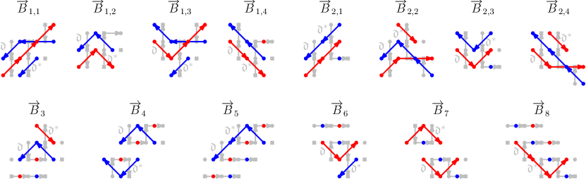
Figure 19. The blockades of Lemma 6.3 represented in terms of oriented TFPLs and in terms of blue-red path tangles.

Proof.

In the following, for $(i,j)=(1,1),(1,2),(1,3),(1,4),(2,1),(2,2),(2,3),(3,1),(3,2),(3,3)$ set

$$\#\overrightarrow{ML}_{i,j}(\mathfrak{d}) =|\{0\leq\ell\leq L(\mathfrak{d})-1:\textnormal{ by }\operatorname{WL}\textnormal{ the move }\overrightarrow{M}_{i,j}\textnormal{ is applied to }\mathfrak{d}\textnormal{ in }\operatorname{WL}^{\ell}(\overrightarrow{f})\}|.$$

The numbers $\#\overrightarrow{ML}_{4}^{b}(\mathfrak{d})$, $\#\overrightarrow{ML}_{4}^{t}(\mathfrak{d})$, $\#\overrightarrow{ML}_{5}^{b}(\mathfrak{d})$ and $\#\overrightarrow{ML}_{5}^{t}(\mathfrak{d})$ are defined analogously. Furthermore, set

$$\operatorname{D}_{NW}(\mathfrak{d},\mathfrak{d}^{\ast}) =\sum\limits_{i=1}^{4}\#\overrightarrow{ML}_{1,i}(\mathfrak{d})+\sum\limits_{j=1}^{3}\#\overrightarrow{ML}_{3,j}(\mathfrak{d})+\#\overrightarrow{ML}_{4}^{t}(\mathfrak{d})+\#\overrightarrow{ML}_{5}^{b}(\mathfrak{d})$$

$$-\sum\limits_{i=1}^{4}\#\overrightarrow{ML}_{1,i}(\mathfrak{d}^{\ast})-\sum\limits_{j=1}^{3}\#\overrightarrow{ML}_{3,j}(\mathfrak{d}^{\ast})-\#\overrightarrow{ML}_{4}^{t}(\mathfrak{d}^{\ast})-\#\overrightarrow{ML}_{5}^{b}(\mathfrak{d}^{\ast}),$$

$$\operatorname{D}_{NE}(\mathfrak{d},\mathfrak{d}^{\ast}) =N-\operatorname{HeightL}(\mathfrak{d})-\sum\limits_{i=1}^{4}\#\overrightarrow{ML}_{1,i}(\mathfrak{d})-\sum\limits_{j=1}^{3}\#\overrightarrow{ML}_{2,j}(\mathfrak{d})-\#\overrightarrow{ML}_{4}^{b}(\mathfrak{d})-\#\overrightarrow{ML}_{5}^{t}(\mathfrak{d})$$

$$-N+\operatorname{HeightL}(\mathfrak{d}^{\ast})+\sum\limits_{i=1}^{4}\#\overrightarrow{ML}_{1,i}(\mathfrak{d}^{\ast})+\sum\limits_{j=1}^{3}\#\overrightarrow{ML}_{2,j}(\mathfrak{d}^{\ast})+\#\overrightarrow{ML}_{4}^{b}(\mathfrak{d}^{\ast})+\#\overrightarrow{ML}_{5}^{t}(\mathfrak{d}^{\ast}),$$

$$\operatorname{Red}(\mathfrak{d},\mathfrak{d}^{\ast}) =L_{1}(v^{L(\mathfrak{d})})-\#\overrightarrow{ML}_{1,1}(\mathfrak{d})-\#\overrightarrow{ML}_{1,4}(\mathfrak{d})-\#\overrightarrow{ML}_{2,3}(\mathfrak{d})+\#\overrightarrow{ML}_{3,3}(\mathfrak{d})-\#\overrightarrow{ML}_{4}^{b}(\mathfrak{d})$$

$$-L_{1}(v^{L(\mathfrak{d}^{\ast})})+\#\overrightarrow{ML}_{1,1}(\mathfrak{d}^{\ast})+\#\overrightarrow{ML}_{1,4}(\mathfrak{d}^{\ast})+\#\overrightarrow{ML}_{2,3}(\mathfrak{d}^{\ast})-\#\overrightarrow{ML}_{3,3}(\mathfrak{d}^{\ast})+\#\overrightarrow{ML}_{4}^{b}(\mathfrak{d}^{\ast}),$$

$$\operatorname{Blue}(\mathfrak{d},\mathfrak{d}^{\ast}) =\#\overrightarrow{ML}_{1,2}(\mathfrak{d})+\#\overrightarrow{ML}_{1,3}(\mathfrak{d})-\#\overrightarrow{ML}_{2,3}(\mathfrak{d})+\#\overrightarrow{ML}_{3,3}(\mathfrak{d})-\#\overrightarrow{ML}_{4}^{b}(\mathfrak{d})$$

$$-\#\overrightarrow{ML}_{1,2}(\mathfrak{d}^{\ast})-\#\overrightarrow{ML}_{1,3}(\mathfrak{d}^{\ast})+\#\overrightarrow{ML}_{2,3}(\mathfrak{d}^{\ast})-\#\overrightarrow{ML}_{3,3}(\mathfrak{d}^{\ast})+\#\overrightarrow{ML}_{4}^{b}(\mathfrak{d}^{\ast}).$$

An easy computation shows that

$$\operatorname{D}_{NW}(\mathfrak{d},\mathfrak{d}^{\ast})-\operatorname{Blue}(\mathfrak{d},\mathfrak{d}^{\ast})-\operatorname{D}_{NE}(\mathfrak{d},\mathfrak{d}^{\ast})+\operatorname{Red}(\mathfrak{d},\mathfrak{d}^{\ast})=L(\mathfrak{d})-L(\mathfrak{d}^{\ast})-L_{0}(v^{L(\mathfrak{d})})+L_{0}(v^{L(\mathfrak{d}^{\ast})}).$$

It remains to show that the lefthand side of the above equation equals $1$. For that purpose, alternative interpretations of the integers $\operatorname{D}_{NW}(\mathfrak{d},\mathfrak{d}^{\ast})$, $\operatorname{D}_{NE}(\mathfrak{d},\mathfrak{d}^{\ast})$, $\operatorname{Red}(\mathfrak{d},\mathfrak{d}^{\ast})$ and $\operatorname{Blue}(\mathfrak{d},\mathfrak{d}^{\ast})$ are considered which derive from Lemma 5.7.

From now on, consider the blue-red path tangle associated with $\operatorname{WL}(\overrightarrow{f})$ for each $0\leq\ell\leq L(\mathfrak{d})$. As a start, $\operatorname{D}_{NW}(\mathfrak{d},\mathfrak{d}^{\ast})$ equals the difference of the number of $\backslash$-diagonals of red vertices to the right of the one whereon the center of the down step corresponding to $\mathfrak{d}$ lies and the number of $\backslash$-diagonals of red vertices to the right of the one whereon the center of the down step corresponding to $\mathfrak{d}^{\ast}$ lies by the same arguments as in the proof of Lemma 5.7(1).

Furthermore, $\operatorname{D}_{NE}(\mathfrak{d},\mathfrak{d}^{\ast})$ equals the number of $/$-diagonals of blue vertices to the left of the one whereon the center of the down step corresponding to $\mathfrak{d}$ lies and the number of $/$-diagonals of blue vertices to the left of the one whereon the center of the down step corresponding to $\mathfrak{d}^{\ast}$ lies by the same arguments as in the proof of Lemma 5.7.

Next, $\operatorname{Red}(\mathfrak{d},\mathfrak{d}^{\ast})$ equals the difference of the number of red paths $\mathfrak{d}$ ”jumps over” in the process of moving to the left boundary by repeatedly applying right-Wieland drift and the number of red paths $\mathfrak{d}^{\ast}$ ”jumps over” in the process of moving to the left boundary by the iterated application of right-Wieland drift by the same arguments as in the proof of Lemma 5.7(3). To be more precise, a blue down step “jumps over” a red path by the application of $\operatorname{WR}$ if before the application of $\operatorname{WR}$ it is in the area below the red path and after the application it is in the area above the red path. On the other hand, a red down step “jumps over” a red path if after the application of $\operatorname{WR}$ it is a blue down step that lies in the area above the red path.

Finally, $\operatorname{Blue}(\mathfrak{d},\mathfrak{d}^{\ast})$ is the difference of the number of blue paths $\mathfrak{d}$ ”jumps over” in the process of moving to the right boundary by repeatedly applying left-Wieland drift and the number of blue paths $\mathfrak{d}^{\ast}$ ”jumps over” in the process of moving to the right boundary by the iterated application of left-Wieland drift by the same arguments as in the proof of Lemma 5.7(4). To be more precise, a red down step “jumps over” a blue path by the application of $\operatorname{WL}$ if before the application of $\operatorname{WL}$ it lies in the area below the blue path and after the application it is in the area above the blue path. On the other hand, a blue down step “jumps over” a blue path if after the application of $\operatorname{WL}$ it is a red down step that lies in the area above the red path.

Thus, for each blockade the integers $\operatorname{D}_{NW}(\mathfrak{d},\mathfrak{d}^{\ast})$, $\operatorname{D}_{NE}(\mathfrak{d},\mathfrak{d}^{\ast})$, $\operatorname{Red}(\mathfrak{d},\mathfrak{d}^{\ast})$ and $\operatorname{Blue}(\mathfrak{d},\mathfrak{d}^{\ast})$ can be computed separately by looking at Figure 19. In Table 4, $\operatorname{D}_{NW}(\mathfrak{d},\mathfrak{d}^{\ast})$, $\operatorname{D}_{NE}(\mathfrak{d},\mathfrak{d}^{\ast})$, $\operatorname{Red}(\mathfrak{d},\mathfrak{d}^{\ast})$ and $\operatorname{Blue}(\mathfrak{d},\mathfrak{d}^{\ast})$ are listed.

	$\overrightarrow{B}_{1,1}$	$\overrightarrow{B}_{1,2}$	$\overrightarrow{B}_{1,3}$	$\overrightarrow{B}_{1,4}$	$\overrightarrow{B}_{2,1}$	$\overrightarrow{B}_{2,2}$	$\overrightarrow{B}_{2,3}$	$\overrightarrow{B}_{2,4}$	$\overrightarrow{B}_{3}$	$\overrightarrow{B}_{4}$	$\overrightarrow{B}_{5}$	$\overrightarrow{B}_{6}$	$\overrightarrow{B}_{7}$	$\overrightarrow{B}_{8}$
$\operatorname{D}_{NW}(\mathfrak{d},\mathfrak{d}^{\ast})$	$0$	$0$	$0$	$0$	$1$	$1$	$1$	$1$	$1$	$-1$	$1$	$0$	$1$	$0$
$\operatorname{D}_{NE}(\mathfrak{d},\mathfrak{d}^{\ast})$	$-1$	$-1$	$-1$	$-1$	$0$	$0$	$0$	$0$	$0$	$-1$	$0$	$-1$	$1$	$-1$
$\operatorname{Red}(\mathfrak{d},\mathfrak{d}^{\ast})$	$-1$	$0$	$-1$	$0$	$0$	$1$	$0$	$1$	$1$	$0$	$0$	$-1$	$1$	$0$
$\operatorname{Blue}(\mathfrak{d},\mathfrak{d}^{\ast})$	$-1$	$0$	$-1$	$0$	$0$	$1$	$0$	$1$	$1$	$-1$	$0$	$-1$	$0$	$0$

Table 4. The numbers $\operatorname{D}_{NW}(\mathfrak{d},\mathfrak{d}^{\ast})$, $\operatorname{D}_{NE}(\mathfrak{d},\mathfrak{d}^{\ast})$, $\operatorname{Red}(\mathfrak{d},\mathfrak{d}^{\ast})$ and $\operatorname{Blue}(\mathfrak{d},\mathfrak{d}^{\ast})$ computed separately for each type of blockade.

In summary, it follows that

$$\operatorname{D}_{NW}(\mathfrak{d},\mathfrak{d}^{\ast})-\operatorname{Blue}(\mathfrak{d},\mathfrak{d}^{\ast})-\operatorname{D}_{NE}(\mathfrak{d},\mathfrak{d}^{\ast})+\operatorname{Red}(\mathfrak{d},\mathfrak{d}^{\ast})=1.$$

Therefore, $L(\mathfrak{d})-L(\mathfrak{d}^{\ast})-L_{0}(v^{L(\mathfrak{d})})+L_{0}(v^{L(\mathfrak{d}^{\ast})})=1$. ∎

Proposition 6.2 follows immediately from Lemma 6.4.

Proof of Proposition 6.2.

Let $f$ be an instable TFPL of excess $2$ that contains two drifters $\mathfrak{d}_{\mathfrak{l}}$ and $\mathfrak{d}_{\mathfrak{r}}$ such that $R(\mathfrak{d}_{\mathfrak{r}})\leq R_{1}(u^{R(\mathfrak{d}_{\mathfrak{r}})})$ and $L(\mathfrak{d}_{\mathfrak{l}})\leq L_{0}(v^{L(\mathfrak{d}_{\mathfrak{l}})})$. Without loss of generality, suppose that $\mathfrak{d}_{\mathfrak{l}}$ cannot be moved to the right boundary using the moves $M_{1}$, $M_{2}$ and $M_{3}$. Then, by Lemma 6.4

$$L(\mathfrak{d}_{\mathfrak{l}})\geq L(\mathfrak{d}_{\mathfrak{r}})+L_{0}(v^{L(\mathfrak{d}_{\mathfrak{l}})})-L_{0}(v^{L(\mathfrak{d}_{\mathfrak{r}})})+1.$$

Thus, $L_{0}(v^{L(\mathfrak{d}_{\mathfrak{r}})})>L(\mathfrak{d}_{\mathfrak{r}})$ and equivalently $R(\mathfrak{d}_{\mathfrak{r}})>R_{1}(u^{R(\mathfrak{d}_{\mathfrak{r}})})+1$. That is a contradiction. Therefore, $\mathfrak{d}_{\mathfrak{r}}$ can be moved to the right boundary using the moves $M_{1}$, $M_{2}$ and $M_{3}$.

By vertical symmetry, $\mathfrak{d}_{\mathfrak{l}}$ can be moved to the left boundary by the moves $M_{1}^{-1}$, $M_{2}^{-1}$ or $M_{3}^{-1}$. ∎

In Figure 20, the instable TFPL of excess $2$ of Figure 16 and the triple $(S,g,T)$ associated with it are depicted.

Figure 20. The instable TFPL of Figure 16 and the triple $(S,g,T)$ it is associated with: $S$ is a semi-standard Young tableau of skew shape $\lambda(10110)/\lambda(01101)$, $g$ is a stable TFPL with boundary $(10110,00111;10110)$ and $T$ is the empty semi-standard Young tableau of skew shape $\lambda(00111)^{\prime}/\lambda(00111)^{\prime}$.

Proof of Theorem 1.

Let $u,v,w$ be words of length $N$ satisfying $exc(u,v;w)\leq 2$. Furthermore, let $f\in T_{u,v}^{w}$ be instable and denote by $(S,g,T)$ the image of $f$ under $\Phi$. As a start, $S\in G_{\lambda(u),\lambda(u^{+})}$ for the following reason: let $c$ be a cell of the Young diagram of skew shape $\lambda(u^{+})/\lambda(u)$ then its entry in $S$ has to be $R(\mathfrak{d})+1$ for a drifter $\mathfrak{d}$ in $f$ and it has to hold $R(\mathfrak{d})\leq R_{1}(u^{R(\mathfrak{d})})$ by the definition of $\Phi$. Since $R_{1}(u^{R(\mathfrak{d})})$ is the number of columns to the right of $c$ the entry of $c$ can at most be the number of columns to the right of $c$ plus one. By analogous arguments, $T\in G_{\lambda(v)^{\prime},\lambda(v^{+})^{\prime}}$.

Thus, it remains to show that $\Phi$ is a bijection. This is done by giving the inverse map: let $u^{+}\geq u$, $v^{+}\geq v$, $S\in G_{\lambda(u),\lambda(u^{+})}$, $g\in S_{u^{+},v^{+}}^{w}$ and $T\in G_{\lambda(v)^{\prime},\lambda(v^{+})^{\prime}}$ and consider the sequences

$$\lambda(u)=\lambda(u^{0})\subseteq\lambda(u^{1})\subseteq\cdots\subseteq\lambda(u^{R})\subseteq\lambda(u^{R+1})=\lambda(u^{+})$$

corresponding to $S$ so that $R+1$ is the largest entry of $S$ and

$$\lambda(v)^{\prime}=\lambda(v^{0})^{\prime}\subseteq\lambda(v^{1})^{\prime}\subseteq\cdots\subseteq\lambda(v^{L})^{\prime}\subseteq\lambda(v^{L+1})^{\prime}$$

corresponding to $T$ so that $L+1$ is the largest entry of $T$. Then associate $(S,g,T)$ with a TFPL $\Psi(S,g,T)$ in $T_{u,v}^{w}$ as follows:

1. If $u^{+}>u$ and $v^{+}=v$, then set $\Psi(S,g,T)=(\operatorname{WL}_{u^{0}}\circ\operatorname{WL}_{u^{1}}\circ\cdots\circ\operatorname{WL}_{u^{R-1}}\circ\operatorname{WL}_{u^{R}})(g)$.

2. If $u^{+}=u$ and $v^{+}>v$, then set $\Psi(S,g,T)=(\operatorname{WR}_{v^{0}}\circ\operatorname{WR}_{v^{1}}\circ\cdots\circ\operatorname{WR}_{v^{L-1}}\circ\operatorname{WR}_{v^{L}})(g)$.

3. If $u^{+}>u$ and $v^{+}>v$, then $\Psi(S,g,T)$ is the TFPL obtained from $g$ as follows: since $u^{+}>u$ and $v^{+}>v$ the skew shaped Young diagrams $\lambda(u^{+})/\lambda(u)$ and $\lambda(v^{+})^{\prime}/\lambda(v)^{\prime}$ both consist of precisely one cell. Hence, denote by $j-1$ the number of columns to the right of the one cell $\lambda(u^{+})/\lambda(u)$ contains and by $i_{j}$ the index of the $j$-th one in $u^{+}$. On the other hand, denote by $j^{\prime}-1$ the number of columns to the right of the one cell $\lambda(v^{+})^{\prime}/\lambda(v)^{\prime}$ contains and by $i_{j}^{\prime}$ the index of the $j^{\prime}$-th zero in $v^{+}$. Now, a drifter $\mathfrak{d}_{\mathfrak{l}}$ incident to $L_{i_{j}+1}$ in $g$ is inserted whereas the horizontal edge incident to $L_{i_{j}}$ is deleted, a drifter $\mathfrak{d}_{\mathfrak{r}}$ incident to $R_{i_{j}^{\prime}-1}$ in $g$ is inserted, whereas the horizontal edge incident to $R_{i_{j}^{\prime}}$ is deleted, $\mathfrak{d}_{\mathfrak{l}}$ is moved $L$ times by a move $M_{1}$, $M_{2}$ or $M_{3}$ and $\mathfrak{d}_{\mathfrak{r}}$ is moved $R$ times by a move $M_{1}^{-1}$, $M_{2}^{-1}$ or $M_{3}^{-1}$. The so-obtained TFPL is the image of $(S,g,T)$ under $\Psi$.

4. If $u^{+}=u$ and $v^{+}=v$, then $\Psi(S,g,T)=g$.

It can easily be seen that $\Psi$ is the inverse map of $\Phi$. ∎

References

- [1] S. Beil, I. Fischer and P. Nadeau. Wieland drift for triangular fully packed loop configurations, Elect. J. Comb., 22(1), 2015
- [2] A. Buch. A Littlewood-Richardson rule for the K-theory of Grassmannians. Acta Math., 189(1): 37–78, 2002.
- [3] L. Cantini and A. Sportiello. Proof of the Razumov–Stroganov conjecture, J. Combinanorial Theory Ser. A, 118(5):1549–1574, 2011.
- [4] F. Caselli, C. Krattenthaler, B. Lass and P. Nadeau. On the number of fully packed loop configurations with a fixed associated matching. Elect. J. Comb., 11(2), 2004.
- [5] I. Fischer, P. Nadeau. Fully Packed Loops in a triangle: matchings, paths and puzzles. J. Combinanorial Theory Ser. A, 130: 64–118, 2015.
- [6] A. Knutson. Modern developments in schubert calculus. Talk given at the North Carolina AMS conference in Winston-Salem, September 2011.
- [7] C. Lenart. Combinatorial Aspects of the K-Theory of Grassmannians. Annals of Combinatorics, 4(1): 67-82, 2000.
- [8] P. Nadeau. Fully Packed Loop Configurations in a Triangle. J. Combinanorial Theory Ser. A, 120(8):2164–2188, 2013.
- [9] P. Nadeau. Fully Packed Loop Configurations in a Triangle and Littlewood–Richardson coefficients. J. Combinanorial Theory Ser. A, 120(8):2137–2147, 2013.
- [10] J. Propp. The many faces of alternating–sign matrices. In Discrete models: combinatorics, computation, and geometry (Paris, 2001), Discrete Math. Theor. Comput. Sci. Proc., AA, pages 043–058 (electronic). Maison Inform. Math. Discrèt. (MIMD), Paris, 2001. 45:175–188, 2009.
- [11] J. Thapper. Refined counting of fully packed loop configurations. Séminaire Lotharingien de Combinatoire, 56:B56e:27, 2007.
- [12] B. Wieland. A large dihedral symmetry of the set of alternating sign matrices. Elect. J. Comb., 7(1–3), 2000.
- [13] D. Zeilberger. Proof of the alternating sign matrix conjecture. Elect. J. Comb., 3(2): Research paper 13, 1996.
- [14] J.–B. Zuber. On the counting of Fully Packed Loop Configurations: Some new conjectures. Elect. J. Comb., 11(1): Research paper 13, 15pp, 2004.