Localization in chaotic systems with a single-channel opening

Abstract

We introduce a single-channel opening in a random Hamiltonian and a quantized chaotic map: localization on the opening occurs as a sensible deviation of the wavefunction statistics from the predictions of random matrix theory, even in the semiclassical limit. Increasing the coupling to the open channel in the quantum model, we observe a similar picture to resonance trapping, made of few fast-decaying states, whose left (right) eigenfunctions are entirely localized on the (preimage of the) opening, and plentiful long-lived states, whose probability density is instead suppressed at the opening. For the latter we derive and test a linear relation between the wavefunction intensities and the decay rates, similar to Breit-Wigner law. We then analyze the statistics of the eigenfunctions of the corresponding (discretized) classical propagator, finding a similar behavior to the quantum system only in the weak-coupling regime.

I Introduction

One of the distinctive traits of all chaotic systems is their seemingly ‘random’ behavior EckRu . As a consequence, one usually assumes that the eigenfunctions of a quantized chaotic Hamiltonian have the same statistical properties (i.e. wavefunction intensity distribution) of a complete set of waves with random amplitudes and phases BerryTab ; stoeck , or equivalently, of the eigenvectors of a Hermitian matrix with random entries, according to random matrix theory (RMT) wigner ; Mehta . Due to a number of applications (quantum information theory Prosen ; GeorgShep ; Zurek , classical noeck ; Hentschel and quantum optics AcMiShi ; moore ; embran , quantum transport Benak ; Miao ), as well as to equally many theoretical issues (see for example diff ; Kap_opn ; weyl ), the quantum chaos community is nowadays largely focused on the behavior of open systems Petruccio .

In this paper we address one of the simplest theoretical questions: whether and how the wavefunction statistics deviates from the predictions of the random wave assumption as we perturb a chaotic system with a single-channel opening. As main result of our investigation, we numerically find that the overall wavefunction intensity distribution at the location of the opening does change from the RMT-expected $\chi^{2}-$shape to a longer-tailed curve, which is analytically described using perturbation theory. It physically implies that localization occurs at the opening. In our theory the opening can be an arbitrary state $|a\rangle$ in the Hilbert space, however, in most of our testing models we take it as a coherent state in the phase space. Deviations of the wavefunction statistics from RMT have been observed before in real space: for time- reversally symmetric systems, it was conjectured PniShap and then shown analytically and experimentally Sebaetal that the distribution of the wavefunctions at the leads smoothly crosses over from Porter-Thomas’ to Poisson’s with the coupling to the opening. Although there was no explicit mention of localization, the wavefunction distribution for a two-channel opening was found to be an inverse square-root, of much slower decay than the RMT prediction. In a later work Ishioetal , this behavior was related to the correlations between real and imaginary parts of the wavefunction, which in general may depend on the underlying classical dynamics.

On the other hand, real- and phase-space localization have been detected in closed systems in correspondence of the so-called scars Hel84 ; kap_hel . Within that framework, the distribution of the intensities on an unstable periodic orbit was found to decay slower than the RMT-expected kap_prl , due to a phenomenon of constructive interference. This is not our case: in order to rule out scarring, we place our probe states away from periodic orbits. Still, the localization found for weak coupling to the opening does hold in the semiclassical limit, which makes us think of a classical effect.

Successively, we follow the evolution of the wavefunction statistics of the quantum map for strong coupling to the opening. As a result, the intensity distribution becomes separated into several long-lived- and a few short-lived eigenstates. We show that their intensities are proportional to their decay rates, arguing that this quantum effect can be explained with the existing theories on resonance trapping rotter91 ; russky . In particular, the intensities of the long-lived states depend on the escape rates through a linear relation akin to Breit-Wigner law stoeck .

In the second part of the paper we perform analogous simulations on the classical cat map and, by looking at the statistics of the eigenfunctions of the classical propagator (Perron-Frobenius operator chaosbook ), we find the deviation from the closed system in all similar to the quantum case for weak coupling to the opening. This observation corroborates the hypothesis of a classical mechanism behind localization, in this regime. On the contrary, we show that a strongly-coupled opening does not result in resonance-trapping, which makes the classical setting substantially different from the quantum, in this regime.

The paper is organized as follows: in section II.1 we calculate the deviation of the wavefunction statistics from an exponential distribution due to a single-channel opening by using first-order perturbation theory. In section II.2 we verify the theoretical expectation using random Hamiltonians drawn from the Gaussian unitary ensemble (GUE) Mehta , and successively on the eigenfunctions of the quantized cat map creagh . Section II.3 deals with the strong-coupling regime: we analyze the proportionality between escape rates and intensities, while we account for the localization patterns of left and right fastest-decaying eigenfunctions in section II.4. In section III we introduce the Perron-Frobenius operator of the same test-map as a classical propagator, and numerically demonstrate an analogous deviation from RMT of its eigenfunction statistics for both weak and strong couplings to a small opening in the phase space. Summary and conclusions are given in section IV.

II Wavefunction intensity distribution

II.1 Theory

Suppose $H_{0}$ is a GUE Hamiltonian. Since its eigenfunctions are complex valued, their intensities $x=|\langle a|\psi_{0}\rangle|^{2}$ at a certain state $|a\rangle$ follow the exponential distribution stoeck

$$P(x)=e^{-x}.$$ (1)

Now we open the system at $|a\rangle$ Kap_opn

$$H=H_{0}-i\frac{\Gamma}{2}|a\rangle\langle a|,$$ (2)

and ask how the distribution of intensities $z=|\langle a|\psi\rangle|^{2}$ is changed with respect to the exponential, when $\Gamma$ is small enough. By using perturbation theory schomerus ; polietal ; polirap ; newrussky , we expand the amplitudes $\langle a|\psi\rangle$ in the first order as

$$\left<a|\psi_{n}\right>\simeq\left<a|\psi_{n}^{0}\right>-i\Gamma\left<a|\psi_{n}^{0}\right>\sum_{p\neq n}\frac{|\left<\psi_{p}^{0}|a\right>|^{2}}{2(E_{n}-E_{p})}.$$ (3)

Left and right eigenfunctions are in general distinct for the non-hermitian operator (2), but they are just the complex conjugate of each other in first-order perturbation regime. We recognize two uncorrelated quantities, $\xi\equiv\left<a|\psi^{0}_{n}\right>$ whose real and imaginary parts are Gaussian distributed , and $\eta\equiv\sum_{p\neq n}\frac{|\left<\psi_{p}^{0}|a\right>|^{2}}{2(E_{n}-E_{p})}$, following

$$P_{1}(\eta)\propto\left(\frac{1}{1+\gamma^{2}\eta^{2}}\right)^{2}$$ (4)

with $\gamma=\Delta E\pi^{-1}$, and $\Delta E$ average level spacing of $H_{0}$ (derivation in Appendix A and schomerus ). We seek the distribution of the variable $z\equiv|\langle a|\psi\rangle|^{2}=\xi^{2}+\Gamma^{2}\xi^{2}\eta^{2}$, namely

$$P(z) = \int d\xi d\eta\delta\left(z-\xi^{2}-\Gamma^{2}\xi^{2}\eta^{2}\right)P_{0}(\xi)P_{1}(\eta)$$ (5)

$$= \frac{2\gamma}{\pi}\int\frac{d\eta e^{-z/(1+\Gamma^{2}\eta^{2})}}{(1+\gamma^{2}\eta^{2})^{2}(1+\Gamma^{2}\eta^{2})},$$

where $P_{0}(\xi)\propto e^{-\xi^{2}}$. We immediately see that its expectation value

$$\langle z\rangle=\frac{\Gamma^{2}+\gamma^{2}}{\gamma^{2}}$$ (6)

always exceeds unity, meaning the opening produces a longer tail, and therefore a certain amount of localization of the probability density takes place.

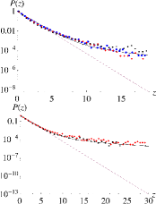
Figure 1: (a) Rescaled sample distributions of the overall wavefunction intensities $P\left(z=|\left<a|\psi\right>|^{2}\right)$ in log scale, obtained diagonalizing several realizations of a GUE Hamiltonian, for: $N=16384$ (dots, $8$ realizations), $N=4096$ (diamonds, $18$ realizations), $N=200$ (squares, $600$ realizations), and loss parameter $\Gamma=0.5$; solid and dashed lines are the theoretical expectation (5) and the exponential distribution (1), respectively. (b) The same analysis with the quantum cat map (14): $N=4096$ (diamonds, $28$ realizations), $N=200$ (squares, $600$ realizations), and $\Gamma=1$.

II.2 Numerical tests

We now verify the theoretical intensity distribution (5) first by diagonalizing multiple realizations of the non-Hermitian Hamiltonian (2), where both $H_{0}$ and the amplitudes $\left<a|\psi_{n}^{0}\right>$ are drawn from the Gaussian unitary ensemble (GUE). The resulting probability distribution for the wavefunction intensities $|\left<a|\psi\right>|^{2}$ in first-order perturbation regime agrees with the expression (5) as shown in the example of Fig. 1(a). The dimension of the Hilbert space chosen ranges from $N=200$ to $N=16384$, suggesting that the result holds in the semiclassical lmit. We will go back to this issue in sec. III.

Figure 1(b) shows that our prediction for a perturbed GUE Hamiltonian also fits the distribution of the wavefunction intensities of the quantized kicked cat map with a small opening. The classical evolution of the cat map reads creagh ; Cr_Lee

$$F_{\epsilon}=F_{0}\circ M_{\epsilon},$$ (7)

with

$$F_{0}:\left(\begin{array}[]{cc}q^{\prime}\\ p^{\prime}\end{array}\right)=\left(\begin{array}[]{cc}1&1\\ 1&2\end{array}\right)\left(\begin{array}[]{cc}q\\ p\end{array}\right)\hskip 8.5359pt\text{mod}1,$$ (8)

and

$$M_{\epsilon}:\left(\begin{array}[]{cc}q^{\prime}\\ p^{\prime}\end{array}\right)=\left(\begin{array}[]{cc}q-\epsilon\sin(2\pi p)\\ p\\ \end{array}\right)\hskip 8.5359pt\text{mod}1$$ (9)

The quantization of the map is given by creagh ; han_ber

$$U_{\epsilon}=U_{0}V_{\epsilon}$$ (10)

where

$$\left<q_{j}|U_{0}|q_{k}\right>=N^{-1/2}\text{e}^{i\pi/4}\text{e}^{2\pi Ni(q_{j}^{2}-q_{j}q_{k}+q_{k}^{2}/2)}$$ (11)

and

$$\left<q_{j}|V_{\epsilon}|q_{k}\right>=\sum_{p_{m}}\frac{1}{N}\text{e}^{Ni\left(-\epsilon\cos 2\pi p_{m}+2\pi(q_{j}-q_{k})p_{m}\right)}.$$ (12)

The quantization of the linear map (8) is known to possess pseudo-symmetries KeatMez that make the spectral statistics deviate from the Circular Unitary Ensemble (CUE), hence the use of the perturbation (9) to restore the RMT behavior. Here the opening is a minimum-uncertainty Gaussian wavepacket

$$\left<q|a\right>=\left(\frac{1}{\pi\hbar^{2}}\right)^{1/4}\text{e}^{-(q-q_{0})^{2}/2\hbar+ip_{0}(q-q_{0})/\hbar},$$ (13)

whose center $(q_{0},p_{0})$ is chosen at random on the unit torus (the scar at the origin Cr_Lee ; LRLK is carefully avoided). The non-unitary propagator is realized by replacing $U_{\epsilon}$ of (10) with Kap_opn ; LRLK

$$U=\left(1-\frac{\Gamma}{2}\left|a\right>\left<a\right|\right)U_{\epsilon}.$$ (14)

All the steps of the derivation of Eq. (5) would still hold in this case, except for Eq. (4), since the quasienergies of the cat map follow the statistics of the CUE, instead of the GUE’s. Still, both are asymptotically equivalent for $N\rightarrow\infty$ Mehta . In our simulations we alternatively set $N=200$ and $4096$, and produce an ensemble statistics of over $10^{5}$ states, by repeatedly diagonalizing the matrix (14) over different values of the kick strength $\epsilon$, chosen at random within the range $[0.1,0.2]$.

II.3 Strong coupling to the opening

When we further increase the coupling $\Gamma$ in the propagator (14), the curve (5) no longer fits the numerical data, as we leave the perturbation regime. A few short-lived left eigenstates are localized on the opening, while the rest are characterized by intensity suppression together with small decay rates. We will clarify the localization patterns of left and right eigenfunctions in section II.4, while we focus for the moment on the left ones. The overlaps between the open region and the eigenstates are presented as a function of the decay rate in Fig. 2(a), reminiscent of the so-called ‘resonance trapping’ effect rotter91 ; kleinrot ; russky ; rotlet ; RPPS ; per_rot ; isra ; rotteralone ; stockexp , whose main results we summarize as follows.

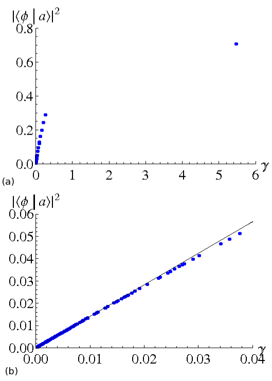
Figure 2: (a) Overlaps between the opening and the left eigenfunctions of the quantized cat map vs. decay rates $\gamma$, showing the resonance trapping effect. (b) The linear part of the data is well described by Eq. (18), here $\Gamma=2\sqrt{2}$.

Consider the complex eigenvalues of $H$, $E_{n}-i\gamma_{n}$, $\gamma_{n}$ being the decay rates. It has been observed and explained rotlet ; russky that when the overall loss $w=\sum_{n}\gamma_{n}$ is greater than the energy range $\Delta E$ where the levels are located, there exists one particularly short-lived state $|\psi_{1}\rangle$, having decay rate $\gamma_{1}=w-O\left(\Delta E/w\right)$, while the rest of the modes have $\gamma_{n\neq 1}=O\left(\Delta E/w\right)$, so that they are ‘trapped’ near the real axis, although still complex valued. We will now use this property together with a $P-Q$ projection formalism to explain the linear dependence of the intensities $|\langle\phi_{n\neq 1}|a\rangle|^{2}$ on the decay rates in this regime. Let $PHP$ be the projection of the Hamiltonian onto the fast-decaying state, $P=|\psi_{1}\rangle\langle\phi_{1}|$, and $QHQ$ the projection on the remaining states, $Q=\sum_{n\neq 1}|\psi_{n}\rangle\langle\phi_{n}|$. We first write an eigenvalue of $QHQ$ as

$$(E_{j}-i\gamma_{j}) = \langle\phi_{j}|QHQ|\psi_{j}\rangle$$ (15)

$$= \langle\phi_{j}|QH_{0}Q|\psi_{j}\rangle-i\frac{\Gamma}{2}\langle\phi_{j}|Q|a\rangle\langle a|Q|\psi_{j}\rangle.$$

On the other hand, we know that $QHQ$ is almost hermitian, so that, to a very good approximation,

$$\left(Q|\psi_{j}\rangle\right)^{\dagger}=\langle\phi_{j}|Q.$$ (16)

We can now recognize the eigenvalues as

$$E_{j}-i\gamma_{j}\simeq\langle\phi_{j}|H_{0}|\phi_{j}\rangle-i\frac{\Gamma}{2}|\langle a|\phi_{j}\rangle|^{2},$$ (17)

where the first term is the expectation value of a hermitian operator, hence a real number, and therefore

$$\gamma_{j}=\frac{\Gamma}{2}|\langle a|\phi_{j}\rangle|^{2},$$ (18)

so that we ‘return’ to a Breit-Wigner kind-of law, as verified in Fig. 2(b) for the simulations of the cat map.

II.4 Left and right eigenfunctions

We notice that in the strong-coupling regime the left and right eigenfunctions of the propagator (14) are well distinct. In particular, we show in Fig. 3 the Husimi distributions of the fastest-decaying eigenstates, whose left eigenfunctions only are supported on the opening. This is explained as follows.

The discrete-time evolution operator (14) is indeed split into unitary evolution $U_{0}$, and a projection describing the opening, $P_{o}=1-|a\rangle\langle a|$, so that $U=P_{o}U_{0}$. Given the eigenvalue $\lambda_{j}$ and its eigenfunctions $\langle\phi_{j}|$ and $|\psi_{j}\rangle$,

$$\langle\phi_{j}|P_{o}U_{0}|x\rangle = \lambda_{j}^{*}\langle\phi_{j}|x\rangle$$

$$\langle x|P_{o}U_{0}|\psi_{j}\rangle = \lambda_{j}\langle x|\psi_{j}\rangle,$$ (19)

the projection $P_{o}$ acts first on the left eigenfunction, so that in order for the loss to be maximal the amplitudes $\langle\phi_{j}|x\rangle$ should be supported on the opening, in our case the coherent state $|a\rangle$. On the other hand, the unitary propagator $U_{0}$ acts first on the right eigenfunction $|\psi_{j}\rangle$: in one time step we approximate the quantum evolution with the classical map $F(x)$, and

$$|\langle x|U_{0}|\psi_{j}\rangle|^{2}\simeq|F(\psi_{j}(x))|^{2},$$ (20)

so that loss/decay rate are highest if $|\psi_{j}\rangle$ is supported on the classical preimage of the opening, $F^{-1}(o)$ Schom_Tword ; LRLK (Fig. 3). The localization patterns of left and right eigenfunctions will differ most when they occur where the system is more sensitive to initial conditions, typically away from fixed points or stable/unstable manifolds of the classical map.

In general the outcomes depend on how the propagation and the loss are arranged, which is usually $U=P_{o}U_{0}$ as in our model, but can be inverted sometimes fyod_somm .

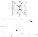
Figure 3: (Top) Husimi distribution of the fastest decaying eigenstate of the quantized cat map, and (bottom) the left and right eigenfunctions the same mode, when the map is open with loss parameter $\Gamma=2\sqrt{2}$. The opening is placed exactly at the position where the Husimi distribution of the left eigenfunction is localized.

III Classical system

In this section we consider a classical chaotic map with a small opening, again looking for deviations from RMT of the sample distributions of the wavefunction intensities, properly defined. The idea is to fit the numerical data with analytic formulae obtained equivalently to (5) in perturbation regime, to then extend the analysis to a strongly-coupled opening, as done in the quantum setting.

Using the density operator $\hat{\rho}$, the wavefunction intensities in the quantum regime can be written as

$$|\langle a|\psi\rangle|^{2}=\langle a|\hat{\rho}|a\rangle.$$ (21)

Here $\hat{\rho}$ obeys the Liouville-von Neumann equation Sakurai

$$i\hbar\partial_{t}\hat{\rho}=[H,\hat{\rho}],$$ (22)

whose classical analog is goldie

$$\partial_{t}\rho=\{H,\rho\}.$$ (23)

The classical Liouville propagator can be written as

$$U^{t}_{cl}=e^{i\hat{L}t},$$ (24)

where $\hat{L}=\{H,\cdot\}$ is the Liouville differential operator. In the Hamiltonian case $\hat{L}^{\dagger}=-\hat{L}$, and therefore the evolution (24) is unitary. The classical evolution operator is supported on a space of generalized functions, and its the spectrum has a discrete and a continuous part (Stone’s theorem); all the eigenfrequencies lie on the unit circle. In particular, ergodic and mixing systems only have one isolated eigenvalue, $e^{i\omega_{0}}=1$, while the rest of the spectrum is continuous Gaspard .

In reality every system experiences noise, coming for example from uncertainties or roundoff errors. However small, noise breaks unitarity and changes the spectrum of the Liouville propagator, from continuous to discrete gasp95 . The (‘leading’) unit eigenvalue is still there, but the rest of the spectrum moves inside the unit circle. In a closed system, the ground-state eigenfunction of eigenvalue equal to unity (natural measure) is real and positive definite, the density to which all initial conditions asymptotically converge. The other eigenfunctions are in general complex and called ‘relaxation modes’, as they are associated with the decay of correlations chaosbook :

$$\langle g|{\cal L}|f\rangle=\sum e^{-\gamma_{n}}\langle g|\rho_{n}\rangle\langle\tilde{\rho}_{n}|f\rangle$$ (25)

The classical-to-quantum correspondence was studied by Fishman and coworkers fish ; fish_clique , who found that the formal solution to the classical Liouville equation, called Perron-Frobenius operator [here $x=(q,p)$]

$$\left({{\cal L}}^{t}\circ\rho\right)(x)={\int_{\cal M}{\!d{x_{0}}}\>}\delta\negthinspace\left({x-{f^{t}({x_{0}})}}\right)\rho({x_{0}},0),$$ (26)

when discretized, effectively behaves like the weakly noisy operator, and has the same spectrum as the quantum propagator of the Wigner function in the classical limit (a similar result was shown in PaLuSr ).

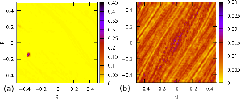
Figure 4: Absolute values of (a) a fast- and (b) a slow-decaying eigenfunctions of the evolution operator (26) for the open cat map (7), with the hole located in the square $[-0.4,-0.3]\times[-0.2,-0.1]$, obtained diagonalizing a $10^{4}\times 10^{4}$ discretization (29). The manifold structure of the cat map is shown in (b).

Based on that, we can say that the noise introduced by the discretization washes out the fine details of the chaotic dynamics, and makes the random-wave assumption hold for the eigenfunctions of (26). These are complex valued (in the phase space), and therefore their squared magnitudes (‘intensities’) $|\rho_{n}(x)|^{2}$ follow a $\chi^{2}$ distribution. Ideally, the classical limit of the minimum-uncertainty wave packet would correspond to just one cell of the phase-space discretization. Here we want to repeat the analysis carried in the quantum setting, and appreciate the difference in the statistics of the eigenfunctions from the closed to the open system. We believe this is done most effectively by taking the sum of the square magnitudes over a small phase-space interval, as

$$\xi_{n}=\int_{{\cal M}_{o}}dx_{0}\int dx|\rho_{n}(x)|^{2}\delta(x-x_{0}),$$ (27)

that is the overlap of $|\rho_{n}(x)|^{2}$ with a delta function [classical limit of the coherent state $|a\rangle$ of Eq. (13)] supported on the probing region ${\cal M}_{o}$. The quantum analog of Eq. (27) would be $\sum_{a^{\prime}}|\langle a^{\prime}|\psi\rangle|^{2}$, over a number of probe states. In that case, the probability density $P\left(\sum_{a^{\prime}}|\langle a^{\prime}|\psi\rangle|^{2}\right)$ for the unperturbed system is a $\chi^{2}-$distribution with $M$ degrees of freedom,

$$P_{M}(\xi)=\frac{\xi^{M/2-1}e^{-\xi/2}}{\Gamma\left(\frac{1}{2}M\right)2^{M/2}},$$ (28)

which becomes a Gaussian as $M\rightarrow\infty$.

We then perform numerical simulations on the classical cat map (7): the Perron-Frobenius operator is discretized with Ulam method ulam

$$[{\cal L}]_{ij}\,=\,\frac{1}{|{\cal M}_{i}|}\int_{{\cal M}_{i}}\!dx\int_{{\cal M}_{j}}\!dy\,\delta(y-f(x))\,.$$ (29)

The entries $[{\cal L}]_{ij}$ are estimated using a straightforward Monte Carlo technique ErmShep , based on counting how many trajectories starting from each ${\cal M}_{j}$ land in ${\cal M}_{i}$. A partial opening is realized by randomly decreasing the number of trajectories that start from the hole, which overall covers a tiny $1\%$ of the available phase space. The $10^{4}\times 10^{4}$ matrix (29) is then diagonalized. Fig. 4(a) shows a fast-decaying eigenfunction peaked in correspondence of the hole, as an extreme case of density enhancement at the opening. We then measure the statistics of the intensities (27) in both the closed and open systems (Fig. 5): while the sample taken from the closed system agrees with the law (28) ($M$ is fitted from the data), the ‘intensities’ on the opening exhibit a longer tail, like in the quantum regime. We qualitatively account for this observation by performing the convolution (5) on the unperturbed distribution (28), this time in $M$ degrees of freedom,

$$P(z)\propto\int r^{M-1}drd\eta\delta\left(z-r^{2}-\tilde{\Gamma}^{2}r^{2}\eta^{2}\right)e^{-r^{2}/2}P_{M}(\eta),$$ (30)

where $r^{2}=\sum_{x}|\rho_{n}(x)|^{2}$ (here $x$ is discretized by our grid), while the perturbation $\eta$ follows schomerus

$$P_{M}(\eta)\propto\left(\frac{1}{1+\gamma^{2}\eta^{2}}\right)^{1+M/2}.$$ (31)

The outcome is

$$P_{M}(z)=C_{M}\int d\eta\frac{z^{M/2-1}e^{-z/2(1+\tilde{\Gamma}^{2}\eta^{2})}}{(1+\tilde{\Gamma}^{2}\eta^{2})^{M/2}(1+\gamma^{2}\eta^{2})^{1+M/2}}$$ (32)

where $\gamma=\pi^{-1}$, $C_{M}=\frac{2^{-1-M/2}M}{\pi^{3/2}\Gamma\left(\frac{1+M}{2}\right)}$, while $\tilde{\Gamma}$ is fitted from the sample distribution.

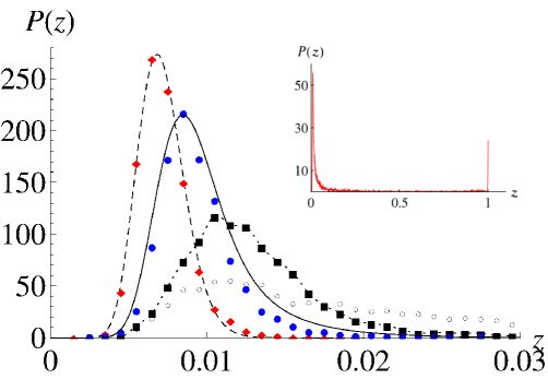
Figure 5: Sample distributions of the intensities $\xi$ [given by Eq. (27)] of the eigenfunctions of the Perron-Frobenius operator for the cat map (7): (diamonds) closed system; (filled dots) $25\%$ partial opening; (squares) $50\%$ partial opening; (empty dots) $75\%$ partial opening; (dashed curve) Eq. (28) rescaled to the data set, where the number of degrees of freedom has been fitted from the data to $M=46$; (solid curve) Eq. (32) with $M=46$, while $\tilde{\Gamma}=1$ is fitted from the data. Inset: total opening at the same location; the peak at the tail represents the instantaneous-decay states.

Fig. 5 also shows two sample distributions of the intensities obtained for stronger couplings to the opening, away from the perturbation regime: importantly, the trend of a flatter curve with a longer tail stays qualitatively the same, indicating an increasing number of fast-decaying states. A total opening introduces a number of instantaneous-decay states Schom_Tword that completely localize on the hole. That generates a peak at the very tail of the sample distribution, whose shape remains otherwise qualitatively the same as for the partial openings (inset of Fig. 5, note the scale). As seen, the quantum system in the same regime behaves differently, as the states that do not decay instantaneously are instead long-lived, and the overall intensity distribution is consistent with the resonance-trapping picture.

We may now give an interpretation of our findings. An open system, be it classical or quantum, must allow for some fast-decaying initial conditions, among the others. Densities and wave functions must be expressible in terms of the eigenstates of the linear operators we are using. As a consequence, some of these eigenstates also decay fast and are more concentrated on the opening and its preimages Schom_Tword . For weak coupling, both classical and quantum simulations fit this physical picture, and behave likewise. Moreover, the calculated deviations of the intensity distributions from the RMT results all rely on perturbation theory, which can be applied to any linear operator with a discrete, non-degenerate spectrum. That is the case for both the quantum Hamiltonian/propagator and the discretized classical evolution operator.

On the other hand, classical and quantum systems behave differently when strongly coupled to the opening, the latter only displaying resonance trapping, while the former not showing any signatures of mode interaction.

IV Summary

We have shown that:

$i)$ The overall wavefunction intensity distribution of a random (GUE) Hamiltonian and a quantized chaotic map deviates from the predictions of RMT, when a weakly-coupled, single-channel opening is introduced. The result holds in the semiclassical limit.

$ii)$ By further increasing the coupling to the open channel in our model, few states localize on the opening particularly strongly and decay fast, while the rest show the opposite behavior: slow decay together with intensity suppression at the opening. Using well-known results in the context of the resonance trapping effect, we derived a linear relation between the intensities of the long-lived states and their decay rates, similar to Breit-Wigner law. In this framework, we also showed that the difference in the localization patterns between fast-decaying left and right eigenfunctions can be recognized as an artifact, inherent of the construction of open quantum maps.

$iii)$ Analogous simulations of the discretized classical evolution operator result in a deviation of the intensity distribution from the RMT expectations akin to what is observed in the quantum setting, when the coupling to the opening is weak enough for perturbation theory to be valid. A stronger coupling to the opening increases the number of fast-decaying states, so as to obtain a longer-tailed intensity distribution, very different from the resonance trapping observed in the quantum simulations.

V Acknowledgements

This research was supported by Basic Science Research Program through the National Research Foundation of Korea (NRF) funded by the Ministery of Science, ICT and future Planning (2013R1A1A2011438). DL acknowledges support from the National Science Foundation of China (NSFC), International Young Scientists (11450110057-041323001).

Appendix A Derivation of Eq. (4)

We start from the joint probability distribution schomerus of $\eta=\sum_{p\neq n}\frac{|\xi|^{2}}{E_{n}-E_{p}}$ and $\zeta=\sum_{p\neq n}\frac{|\xi|^{2}}{(E_{n}-E_{p})^{2}}$,

$$P(\eta,\zeta)\propto\frac{(1+\gamma^{2}\eta^{2})^{M}}{\zeta^{2+3M/2}}e^{-\frac{M\pi}{2\gamma\zeta}\left(1+\gamma^{2}\eta^{2}\right)},$$ (33)

with $M$ number of degrees of freedom. We simply integrate over $\zeta$ to obtain the distribution of $\eta$, in one [Eq. (4)] or $M$ [Eq. (31)] degrees of freedom.

References

- (1) J. P. Eckmann and D. Ruelle, Rev. Mod. Phys. 57, 617 (1985).
- (2) M.V. Berry and M. Tabor, Proc. Roy. Soc. London A 356, 375, 1977.
- (3) H. J. Stöckmann, Quantum Chaos: an Introduction, Cambridge University Press, 1999.
- (4) E. P. Wigner,Group Theory and its Application to the Quantum Mechanics of the Atomic Spectra, (Academic, 1959).
- (5) M. L. Mehta, Random Matrices, Elsevier, 2006.
- (6) T. Prosen, T. H. Seligman, M. Žnidarič, Prog. Theor. Phys. Supp. 150, 200 (2003). T. Prosen, M. Žnidarič, J. Phys. A 34, L681 (2001).
- (7) B. Georgeot, D. L. Shepeliansky, Phys. Rev. Lett. 86, 2890 (2001).
- (8) W. H. Zurek, Rev. Mod. Phys. 75, 715 (2003).
- (9) J. U. Nöckel and A. D. Stone, Nature 385, 45 (1997).
- (10) M. Hentschel and K. Richter, Phys. Rev. E 66, 056207 (2002).
- (11) J. R. Ackerhalt, P. W. Milonni, and M.-L. Shih, Phys. Rep. 128, 205 (1985)
- (12) C. Emary and T. Brandes, Phys. Rev. Lett. 90, 044101 (2003).
- (13) F. L. Moore, J. C. Robinson, C. Bharucha, P. E. Williams, and M. G. Raizen, Phys. Rev. Lett. 73, 2974 (1994). F. L. Moore, J. C. Robinson, C. Bharucha, Bala Sundaram, and M. G. Raizen, ibidem 75, 4598 (1995).
- (14) C. W. J. Beenakker, Rev. Mod. Phys. 69, 731 (1997).
- (15) F. Miao, S. Wijeratne, Y. Zhang, U. C. Coskun, W. Bao, and C. N. Lau, Science 317, 1530 (2007).
- (16) T. A. Brun, I. C. Percival, and R. Schack, J. Phys. A 29, 2077 (1996).
- (17) S. Nonnenmacher, Nonlinearity 24, R123 (2011).
- (18) L. Kaplan, Phys. Rev. E 59, 5325 (1999).
- (19) H. P. Breuer, F. Petruccione, The Theory of Open Quantum Systems, Oxford University Press, 2002.
- (20) R. Pnini and B. Shapiro, Phys. Rev. E 54, R1032 (1996).
- (21) P. Seba, F. Haake, M. Kus, M. Barth, U. Kuhl, and H.-J. Stöckmann, Phys. Rev. E 56, 2680 (1997).
- (22) H. Ishio, A. I. Saichev, A. F. Sadreev, and K.-F. Berggren, Phys. Rev. E 64, 056208 (2001).
- (23) E. Heller, Phys. Rev. Lett. 53, 1515 (1984).
- (24) L. Kaplan, E. J. Heller, Ann. Phys. 264, 171 (1998).
- (25) L. Kaplan, Phys. Rev. Lett. 80 (1998), 2582.
- (26) I. Rotter, Rep. Prog. Phys. 54, 635 (1991).
- (27) V.V. Sokolov and V.G. Zelevinsky, Nucl. Phys. A 504, 562 (1989).
- (28) P. Cvitanović, R. Artuso, R. Mainieri, G. Tanner and G. Vattay, Chaos: Classical and Quantum,ChaosBook.org (Niels Bohr Institute, Copenhagen 2009)
- (29) S.C. Creagh, Chaos 5, 477 (1995).
- (30) H. Schomerus, K. M. Frahm, M. Patra, and C. W. J. Beennakker , Physica A 278, 469 (2000).
- (31) C. Poli, D.V. Savin, O. Legrand, and F. Mortessagne, Phys. Rev. E 80, 46203 (2009).
- (32) C. Poli, O. Legrand, and F. Mortessagne, Phys. Rev. E 82, 055201R (2010).
- (33) Y. V. Fyodorov and D. V. Savin, Phys. Rev. Lett. 108, 184101 (2012).
- (34) S.C. Creagh, S.Y. Lee, and N.D. Whelan, Ann. Phys. 295, 194 (2002).
- (35) J.H. Hannay and M.V. Berry, Physica D 1, 267 (1980).
- (36) J. P. Keating and F. Mezzadri, Nonlinearity 13, 747 (2000).
- (37) D. Lippolis, J.-W. Ryu, S.-Y. Lee, and S. W. Kim, Phys. Rev E 86, 066213 (2012).
- (38) P. Kleinwächter and I. Rotter, Phys. Rev. C 32, 1742 (1985).
- (39) F.-M. Dittes, H. L. Harney, and I. Rotter, Phys. Lett. A 153, 451 (1991).
- (40) I. Rotter, E. Persson, K. Pichugin, and P. Seba, Phys. Rev. E 62, 450 (2000).
- (41) E. Persson and I. Rotter, Phys. Rev. C 59, 164 (1999).
- (42) F. M. Izrailev, D. Saher, and V. V. Sokolov, Phys. Rev. E 49, 130 (1994).
- (43) I. Rotter, Phys. Rev. E 64, 036213 (2001).
- (44) H.-J. Stöckmann et al., Phys. Rev. E 65, 066211 (2002).
- (45) H. Schomerus and J. Tworzydlo, Phys. Rev. Lett. 93, 154102 (2004).
- (46) Y. V. Fyodorov and H.-J. Sommers, JETP Lett. 72, 422 (2000).
- (47) J. J. Sakurai, Modern Quantum Mechanics, Addison-Wesley, 2011.
- (48) H. Goldstein, C. Poole , J. Safko, Classical Mechanics, Addison-Wesley, 2002.
- (49) P. Gaspard, Chaos, Scattering, and Statistical Mechanics, Cambridge University Press, 1999.
- (50) P. Gaspard, G. Nicolis, A. Provata, and S. Tasaki, Phys. Rev. E 51, 74 (1995).
- (51) S. Fishman, in ‘Supersymmetry and Trace Formulae: Chaos and Disorder’, p. 193 (Plenum, 1999).
- (52) M. Khodas, S. Fishman, and O. Agam, Phys. Rev. E 62, 4769 (2000).
- (53) K. Pance, W. Lu, and S. Sridhar, Phys. Rev. Lett. 85, 2737 (2000).
- (54) S.M. Ulam, A Collection of Mathematical Problems, Interscience Publishers, New York 1960.
- (55) L. Ermann and D. L. Shepeliansky, Eur. Phys. J. B 75, 299 (2010).