Compressive Sensing with Prior Support Quality Information and Application to Massive MIMO Channel Estimation with Temporal Correlation

Abstract

In this paper, we consider the problem of compressive sensing (CS) recovery with a prior support and the prior support quality information available. Different from classical works which exploit prior support blindly, we shall propose novel CS recovery algorithms to exploit the prior support adaptively based on the quality information. We analyze the distortion bound of the recovered signal from the proposed algorithm and we show that a better quality prior support can lead to better CS recovery performance. We also show that the proposed algorithm would converge in $\mathcal{O}\left(\log\mbox{SNR}\right)$ steps. To tolerate possible model mismatch, we further propose some robustness designs to combat incorrect prior support quality information. Finally, we apply the proposed framework to sparse channel estimation in massive MIMO systems with temporal correlation to further reduce the required pilot training overhead.

I Introduction

The problem of recovering a sparse signal from a number of compressed measurements has been drawing a lot of attention in the research community [1]. Specifically, consider the following compressive sensing (CS) model:

$$\mathbf{y}=\mathbf{\Phi}\mathbf{x}$$ (1)

where $\mathbf{x}\in\mathbb{C}^{N\times 1}$ is the unknown sparse signal ($||\mathbf{x}||_{0}\ll N$), $\Phi\in\mathbb{C}^{M\times N}$ is the measurement matrix with $M\ll N$ , and $\mathbf{y}\in\mathbb{C}^{M\times 1}$ are the measurements, where the goal is to recover $\mathbf{x}$ based on $\mathbf{y}$ and $\mathbf{\Phi}$. Since $M\ll N$, (1) is in fact an under-determined system and hence there are infinite solutions of $\mathbf{x}$ to satisfy (1) in general. However, utilizing the fact that $\mathbf{x}$ is sparse ($||\mathbf{x}||_{0}\ll N$), it is possible recover $\mathbf{x}$ exactly via the following formulation [1]:

$$\min_{\hat{\mathbf{x}}}||\hat{\mathbf{x}}||_{0}\quad\mbox{s.t.}\,\mathbf{y}=\mathbf{\Phi}\hat{\mathbf{x}}.$$ (2)

Unfortunately, problem (2) is combinatorial and has prohibitive complexity [2]. To have feasible solutions, researchers have designed many methods to approximately solve (2). For instance, the convex approximation approach via $l_{1}$-norm minimization (basis pursuit) is proposed in [2]. Greedy-based algorithms which focus on iteratively identifying the signal support (i.e.,$\mathcal{T}=\{i:\mathbf{x}(i)\neq 0\}$) or approximating the signal coefficients are proposed in [3, 4, 5, 6] (e.g., the orthogonal matching pursuit (OMP) in [3], iterative hard thresholding (IHT) in [4], compressive sampling matching pursuit (CoSaMP) in [5], and subspace pursuit (SP) in [6]). By using the tools of the restricted isometry property (RIP) [2], these CS recovery algorithms [3, 4, 5, 6, 2] are shown to achieve efficient recovery with substantially fewer measurements compared with the signal dimension (i.e., $M\ll N$). Besides, there are also works that deploy the approximate message passing technique to achieve efficient CS recovery [7, 8, 9]. However, they [3, 4, 5, 6, 2, 8, 7, 9] consider one-time static CS recovery and do not exploit the prior information of the signal support.

In practice, we usually encounter the problem of recovering a sequence of sparse signals and the sparse patterns of the signals are usually correlated across time. For instance, consecutive real time video signals [10, 11] usually have strong dependencies. In spectrum sensing, the index set of the occupied frequency band usually varies slowly [12]. In sparse channel estimation, consecutive frames tend to share some multi-paths due to the slowly varying propagation environment between base stations and users [13, 14]. As such, there is huge potential to exploit previously estimated signal support to enhance the CS recovery performance at the present time. In the literature, some works [15, 16, 17, 11, 18] have already considered CS problems with a prior signal support $\mathcal{T}_{0}$ available and modified CS algorithms [15, 16, 17, 11, 18] are proposed to exploit the prior $\mathcal{T}_{0}$ to enhance the performance. For instance, in [15, 16, 17], modified basis pursuit designs are proposed to utilize $\mathcal{T}_{0}$ by minimizing the $l_{1}$-norm of the subvector $\hat{\mathbf{x}}_{\mathcal{T}_{0}^{c}}$ formed by excluding the elements of $\mathbf{x}$ in $\mathcal{T}_{0}$, $\mathcal{T}_{0}^{c}=\{1,...,N\}\backslash\mathcal{T}_{0}$. Based on this, [11, 18] have further considered a weighted $l_{1}$-norm minimization approach to exploit $\mathcal{T}_{0}$. However, these designs [15, 16, 17, 11, 18] do not take the quality of the prior support information $\mathcal{T}_{0}$ into consideration in the problem formulation and fail to exploit $\mathcal{T}_{0}$ adaptively based on the quality of $\mathcal{T}_{0}$. In practice, the prior signal support $\mathcal{T}_{0}$ may contain only part of correct indices for the present time (e.g., practical signal support is temporarily correlated but is also dynamic across time). In cases when only a small part of the indices in $\mathcal{T}_{0}$ is correct, using the modified basis pursuit design in [15, 16, 17, 11] (which fully exploits $\mathcal{T}_{0}$), would lead to a even worse performance [11]. As such, it is desirable to exploit $\mathcal{T}_{0}$ adaptively based on how good $\mathcal{T}_{0}$ is for the present time.

In this paper, we propose a more complete model regarding the prior signal support information. Aside from the prior support $\mathcal{T}_{0}$, we assume that there is a metric to further indicate the quality of $\mathcal{T}_{0}$. Based on this, we design novel algorithms to exploit $\mathcal{T}_{0}$ adaptively based on the quality indicator to achieve better signal recovery performance. Different from previous works [15, 16, 17, 11, 18] with convex relaxation approaches, we shall propose a greedy pursuit approach to achieve our target. To cover more application scenarios, we shall consider a framework with a general signal model which incorporates conventional block sparsity [19, 20] and multiple measurement vector (MMV) joint sparsity models [21, 22, 23]. There are several technical challenges to tackle in this work:

• Algorithm Design to Adaptively Exploit the Prior Support: Note that classical CS works [15, 16, 17, 11, 18] exploit prior support information $\mathcal{T}_{0}$ blindly. To further enhance the recovery performance, we shall design a novel CS algorithm to exploit the prior support $\mathcal{T}_{0}$ adaptively based on the metric information indicating how good $\mathcal{T}_{0}$ is. On the other hand, the proposed CS algorithm should also take the general signal sparsity model into consideration.

• Performance Analysis of the Proposed Algorithm: Besides the algorithm design, it is also important to quantify the performance of the proposed novel CS recovery algorithms. For instance, it is desirable to analyze the distortion bound of the recovered signal and it is desirable to characterize the associated convergence speed of the proposed algorithm.

• Robust Designs to Combat Model mismatch: In practice, there might be occasions with mismatch in the prior support information model (e.g., incorrect information of the prior support quality). For robustness, it it is also desirable to have some alternative robust designs to make sure that the proposed scheme works efficiently even with model mismatch.

In this paper, we shall address the above challenges. In Section II, we introduce the CS problem setup with a general signal sparsity model. We then present a prior support information model and introduce the metric to quantify the quality of the the prior support $\mathcal{T}_{0}$. In Section III, we present the proposed CS algorithm to adaptively exploit the prior support based on the quality indicator. After that, in Section IV, we analyze the recovery performance of the proposed algorithm, and in Section V, we further propose some robust designs to tolerate model mismatch with incorrect prior support quality information. Based on these results, in Section VI, we apply the proposed scheme to sparse channel estimation in massive MIMO systems with temporal correlation, to demonstrate the usefulness of the proposed framework. Numerical results in Section VII demonstrate the performance advantages of the the proposed scheme over the existing state-of-the-art algorithms.

Notations: Uppercase and lowercase boldface letters denote matrices and vectors, respectively. The operators $(\cdot)^{T}$, $(\cdot)^{*}$, $(\cdot)^{H}$, $(\cdot)^{\dagger}$, $|\cdot|$, and $O(\cdot)$ are the transpose, conjugate, conjugate transpose, Moore-Penrose pseudoinverse, cardinality, and big-O notation operator, respectively; $\textrm{supp}(\mathbf{h})$ is the index set of the non-zero entries of vector $\mathbf{h}$; $||\mathbf{A}||_{F}$, $||\mathbf{A}||$ and $||\mathbf{a}||$ denote the Frobenius norm, spectrum norm of $\mathbf{A}$ and Euclidean norm of vector $\mathbf{a}$, respectively.

II System Model

II-A Compressive Sensing Model

Suppose we have compressed measurements $\mathbf{Y}\in\mathbb{C}^{M\times L}$ of an unknown sparse signal matrix $\mathbf{X}\in\mathbb{C}^{N\times L}$ given by

$$\mathbf{Y}=\Phi\mathbf{X}+\mathbf{N}$$ (3)

where $\Phi\in\mathbb{C}^{M\times N}$ ($M\ll N$) is the measurement matrix and $\mathbf{N}\in\mathbb{C}^{N\times L}$ is the measurement noise. Our target is to recover $\mathbf{X}$ based on $\mathbf{Y}$ and $\Phi$. Before we elaborate the recovery algorithm, we first elaborate the considered signal sparsity model and the prior support information for $\mathbf{X}$ in the following sections.

II-B Signal Sparsity Model

Many works have considered CS problems with joint sparsity structures in the literature. For instance, block sparsity is considered in [19, 20] in which the target sparse vector (i.e., $L=1$ in (1)) has simultaneously zero or non-zero blocks with block size $d$. On the other hand, the MMV problem is discussed in [21, 22, 23] where the target sparse matrix ($L>1$) has simultaneously zero or non-zero rows. By exploiting the joint sparsity structures, better recovery performance can be achieved compared with conventional CS algorithms [19, 20, 21, 22, 23]. Motivated by these works, we shall consider a general sparsity model for $\mathbf{X}$ in (3) so that conventional block sparsity or MMV sparsity structure can be incorporated. Suppose the sparse matrix $\mathbf{X}\in\mathbb{C}^{N\times L}$ ($N=Kd$ ) is a concatenation of $K$ chunks where each chunk is of size $d\times L$ and has simultaneously zero or non-zero entries. Denote $\mathbf{X}[k]\in\mathbb{C}^{d\times L}$ as its $k$-th chunk of $\mathbf{X}$ as in Figure 1, i.e.,

$$\mathbf{X}\triangleq\left[\begin{array}[]{cc}\mathbf{X}[1]&\in\mathbb{C}^{d\times L}\\ \mathbf{X}[2]&\in\mathbb{C}^{d\times L}\\ \vdots&\vdots\\ \mathbf{X}[K]&\in\mathbb{C}^{d\times L}\end{array}\right]\in\mathbb{C}^{N\times L},$$ (4)

Define the chunk support $\mathcal{T}$ (with chunk size $d\times L$—assumed throughout the paper) of $\mathbf{X}$ as

$$\mathcal{T}\triangleq\left\{n:\;\left\|\mathbf{X}[n]\right\|_{F}>0,1\leq n\leq K\right\}.$$ (5)

We formally have the following definition of chunk-sparse matrices.

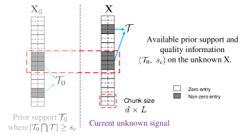
Figure 1: Illustration of the available prior support and quality information $(\mathcal{T}_{0},s_{c})$ for $\mathbf{X}$. Note that $\mathcal{T}_{0}$ (available) and $\mathcal{T}$ (unknown) denote the prior support information and the current signal support, respectively. Our target is to exploit the side information of $(\mathcal{T}_{0},s_{c})$ to improve the CS recovery performance of $\mathbf{X}$ from its compressed measurements $\mathbf{Y}$.

Definition 1 (Chunk Sparsity Level)

Matrix $\mathbf{X}\in\mathbb{C}^{N\times L}$ is said to have $s$-th chunk sparsity level (CSL) if the chunk support $\mathcal{T}$ of $\mathbf{X}$ as in (5) satisfies $|\mathcal{T}|=s\ll K$. ∎

Note that when $d=1$ and $L>1$, the considered signal model is reduced to the MMV joint sparsity models [21, 22, 23]; when $L=1$, the considered signal model is reduced to the block sparsity scenarios [19, 20]; and when both $d=1$ and $L=1$, the considered model degenerates to the classical signal sparsity model without structures [1]. As such, the considered sparse signal model incorporates conventional sparse signal models [21, 22, 23, 19, 20] and potentially covers more application scenarios. Note that practical signals $\mathbf{X}$ may have some joint sparsity (e.g., due to physical collocation [24] or specific application features such as Magnetic resonance imaging [25]) and using a proper signal model enables us to exploit the joint sparsity to enhance the signal recovery performance (as demonstrated in [21, 22, 23, 19, 20]). In this paper, we assume that the CSL of the target signal $\mathbf{X}\in\mathbb{C}^{N\times L}$ is upper bounded by $\bar{s}$, i.e., $|\mathcal{T}|\leq\bar{s}$ and $\bar{s}$ is available, as in classical CS works [5, 6].

II-C Prior Support Information

We consider the following prior support information of $\mathbf{X}$ is available.

Definition 2 (Prior Support Information)

The prior support information regarding the information $\mathbf{X}$ is characterized by a tuple $(\mathcal{T}_{0},s_{c})$, where $s_{c}\leq\left|\mathcal{T}_{0}\right|\leq\bar{s}$, $\left|\mathcal{T}_{0}\bigcap\mathcal{T}\right|\geq s_{c}\geq 0$. ∎

Remark 1 (Interpretation of Definition 2)

Note that $\mathcal{T}_{0}$ denotes the prior signal support and parameter $s_{c}$ is a metric to indicate the quality of the prior support $\mathcal{T}_{0}$. Specifically, a larger $s_{c}$ means that a larger number of indices in $\mathcal{T}_{0}$ is correct and hence means a better quality of $\mathcal{T}_{0}$. Compared with conventional works [15, 16, 17, 11, 18] which exploit $\mathcal{T}_{0}$ blindly, we further consider some uncertainty information about the prior support $\mathcal{T}_{0}$ (quantified by $s_{c}$) and such information allows us to exploit $\mathcal{T}_{0}$ adaptively based on $s_{c}$. Note that $s_{c}$ refers to the number of correct indices but not the specific indices in $\mathcal{T}_{0}\bigcap\mathcal{T}$.

We then summarize the challenge we face in the following and we propose a novel CS algorithm to handle the challenge in the next Section.

Challenge 1: Recover the chunk-sparse matrix $\mathbf{X}$ from $\mathbf{Y}$ in (3) exploiting the prior support information $(\mathcal{T}_{0},\,s_{c})$.

III Algorithm Design to Exploit the Prior Support and Quality Information

In this section, we shall propose a novel CS recovery algorithm to solve Challenge 1 by extending conventional greedy pursuit algorithms with exploitation of $(\mathcal{T}_{0},\,s_{c})$ and adaptation to the chunk sparsity structure of $\mathbf{X}$. Specifically, we select to design from SP [6] from the set of greedy-based CS recovery algorithms, because SP [6] possesses many good properties such as uniform recovery guarantee [6], relatively smaller required RIP constant compared with other schemes of CoSaMP [5] or IHT [4] (based on the so far best known RIP constants for these schemes [26, 27]), and closed-form characterizations on the number of iteration steps [6]. Hence, designing from SP [6] might enable us to obtain similar good properties. Moreover, the manipulations of the support identification in SP [6] provide us an easy interface to incorporate the prior support information $(\mathcal{T}_{0},\,s_{c})$. The detailed algorithm designs are presented in the following.

III-A Algorithm Design

$\mathbf{x}^{\mathcal{T}}$	subvector formed by collecting the
	entries of $\mathbf{x}$ indexed by $\mathcal{T}$.
$\mathbf{X}^{[\mathcal{T}]}$	submatrix formed by collecting the
	chunks of $\mathbf{X}$ indexed by $\mathcal{T}$.
$\Phi_{\mathcal{T}}$	submatrix formed by collecting the
	columns of $\Phi$ indexed by $\mathcal{T}$.
$\Phi_{[\mathcal{T}]}$	submatrices formed by collecting columns
	of $\Phi$ indexed by $\{(k-1)d+1,..,kd:\forall k\in\mathcal{T}\}$.

Table I: Notations.

In [6], a subspace pursuit (SP) algorithm is proposed to solve conventional CS problems. The basic idea of the SP is to keep identifying the signal support based on the maximum correlation criterion [6] and by doing so, the SP algorithm achieves efficient CS recovery with robustness to measurement noises. In this section, we propose a modified subspace pursuit (M-SP) algorithm to solve Challenge 1 with exploitation of $(\mathcal{T}_{0},\,s_{c})$ and adaptation to the chunk sparsity model. To facilitate our presentations, we first define a set of notation rules as in Table I. The details of the proposed M-SP algorithm are presented in Algorithm 1.

Input: $\mathbf{Y}$, $\Phi$, $\bar{s}$, $(\mathcal{T}_{0},s_{c})$, $\gamma$, $d$.

Output: Estimated $\hat{\mathcal{T}}$ and $\hat{\mathbf{X}}$.

Step 1 (Initialization): Initialize the iteration index $l=0$, chunk support$\hat{\mathcal{T}}_{l}=\emptyset$, and the residue matrix $\mathbf{R}_{(l)}=\mathbf{Y}$.

Step 2 (Iteration): Repeat the following steps until stop.

• A (Support Merge): Set $\mathcal{T}_{a}=\hat{\mathcal{T}}_{l}\bigcup\left(\mathcal{T}_{b}\bigcup\mathcal{T}_{c}\right)$, where

  $$\mathcal{T}_{b}=\arg\max_{|\mathcal{T}_{1}|=s_{c},\mathcal{T}_{1}\subseteq\mathcal{T}_{0}}\left\|\left(\Phi^{H}\mathbf{R}_{(l)}\right)^{[\mathcal{T}_{1}]}\right\|_{F}$$ (6)

  $$\mathcal{T}_{c}=\arg\max_{|\mathcal{T}_{2}|=\bar{s}-s_{c},\mathcal{T}_{2}\subseteq\{1,..,K\}\backslash\mathcal{T}_{b}}\left\|\left(\Phi^{H}\mathbf{R}_{(l)}\right)^{[\mathcal{T}_{2}]}\right\|_{F}$$ (7)

• B (LS Estimation): Set $\mathbf{Z}^{[\mathcal{T}_{a}]}=\Phi_{[\mathcal{T}_{a}]}^{\dagger}\mathbf{Y}$ and $\mathbf{Z}^{[\{1,...,K\}\backslash\mathcal{T}_{a}]}=\mathbf{0}$ .

• C (Support Refinement): Select $\hat{\mathcal{T}}_{l+1}$ as follows:

  $$\hat{\mathcal{T}}_{l+1} =\left\{\arg\max_{|\mathcal{T}_{1}|=s_{c},\mathcal{T}_{1}\subseteq\mathcal{T}_{0}}\left\|\mathbf{Z}^{[\mathcal{T}_{1}]}\right\|_{F}\right\}$$

  $$\bigcup\left\{\arg\max_{|\mathcal{T}_{2}|=\bar{s}-s_{c},\mathcal{T}_{2}\subseteq\{1,..,K\}\backslash\mathcal{T}_{1}}\left\|\mathbf{Z}^{[\mathcal{T}_{2}]}\right\|_{F}\right\}$$ (8)

• D (Signal Estimation): Set $\hat{\mathbf{X}}_{(l+1)}^{\left[\hat{\mathcal{T}}_{l+1}\right]}=\Phi_{\left[\hat{\mathcal{T}}_{l+1}\right]}^{\dagger}\mathbf{Y}$ and $\hat{\mathbf{X}}_{(l+1)}^{[\{1,...,K\}\backslash\hat{\mathcal{T}}]}=\mathbf{0}$.

• E (Residue): Compute $\mathbf{R}_{(l+1)}=\mathbf{Y}-\Phi_{\left[\hat{\mathcal{T}}_{l+1}\right]}\hat{\mathbf{X}}_{(l+1)}^{\left[\hat{\mathcal{T}}_{l+1}\right]}$.

• F (Stopping Condition and Output): If $\left\|\mathbf{R}_{(l+1)}\right\|_{F}\leq\gamma$, stop and output $\hat{\mathcal{T}}=\hat{\mathcal{T}}_{l+1}$ and $\hat{\mathbf{X}}=\hat{\mathbf{X}}_{(l+1)}$; Else if $\left\|\mathbf{R}_{(l+1)}\right\|_{F}\geq\left\|\mathbf{R}_{(l)}\right\|_{F}$, stop and output $\hat{\mathcal{T}}=\hat{\mathcal{T}}_{l}$ and $\hat{\mathbf{X}}=\hat{\mathbf{X}}_{(l)}$; Else, set $l=l+1$ and go to Step 2 A.

Algorithm 1 Modified-SP to Solve Challenge 1.

Remark 2 (Interpretation of Algorithm 1)

In the proposed M-SP algorithm (Algorithm 1), $\gamma$ is a threshold parameter, $\hat{\mathcal{T}}_{l}$ and $\hat{\mathbf{X}}_{(l)}$ denote the estimated chunk support and the estimated signal for $\mathbf{X}$ in the $l$-th iteration, respectively. Note that when $d=1$, $L=1$ and $s_{c}=0$, Algorithm 1 will degenerate to conventional SP [6] (except that the M-SP has a different stopping criterion. Table II illustrates the comparison between conventional SP and the proposed M-SP. The following explains how the proposed M-SP exploits the prior support information $(\mathcal{T}_{0},s_{c})$ and adapts to the chunk sparsity model:

• Exploitation of Prior Support Information $(\mathcal{T}_{0},s_{c})$ : Note that the information $(\mathcal{T}_{0},s_{c})$ is utilized in Step 2 A and C of Algorithm 1. As can be seen in Step 2 A, the newly added support (i.e., $\mathcal{T}_{b}\bigcup\mathcal{T}_{c}$) contains two parts, namely $\mathcal{T}_{b}$ and $\mathcal{T}_{c}$, where $\mathcal{T}_{b}$ with size $s_{c}$ is selected from prior support $\mathcal{T}_{0}$, $\mathcal{T}_{c}$ with size $\bar{s}-s_{c}$ is selected from $\{1,..,K\}\backslash\mathcal{T}_{b}$. This design utilizes the fact that prior support $\mathcal{T}_{0}$ contains at least $s_{c}$ correct indices. Similarly, in Step 2 C, the refined signal support $\hat{\mathcal{T}}_{l+1}$ contains two parts, i.e., $s_{c}$ indices from $\mathcal{T}_{0}$ and another $\bar{s}-s_{c}$ from the others. This is in contrast to conventional SP [6] in which the newly added/updated signal support are blindly selected over the entire signal index set $\{1,..,K\}$. Using the proposed support identification criterion, the prior support information $\mathcal{T}_{0}$ is utilized adaptively based on the quality information $s_{c}$, and hence better recovery performance may be achieved.

• Adaptation to the General Sparsity Model: Note that we have considered a general sparsity model in which the signal matrix $\mathbf{X}$ has simultaneous zero or non-zero entries within each chunk (with size $d\times L$). Therefore, instead of identifying each single element in $\mathbf{X}$ separately (as in the conventional SP [6]), we identify each non-zero chunk as a atomic unit based on the aggregate correlation effects between the measurement matrix $\Phi$ and the residue matrix $\mathbf{R}_{(l)}$. For instance, in (6)-(7), we identify a new chunk based on the Frobenius norm of $\left(\Phi^{H}\mathbf{R}_{(l)}\right)^{[\{k\}]}$ which corresponds to an aggregate correlation effect due to the $k$-th chunk. This design adapts to the joint sparsity structure in $\mathbf{X}$ and may achieve better recovery performance [21, 22, 23, 19, 20].

After giving the details of the proposed M-SP algorithm above, it is also important for us to characterize the associated recovery performance. Specifically, we are interested in characterizing the distortion bound of the estimated signal as well as the convergence speed of the proposed M-SP algorithm. We shall discuss these issues in the next Section.

Comparison ($s_{c}=0$, $d=1$, $L=1$)		SP [6, 27]	M-SP
	Performance	covered	covered
no noise	i.e., $\mathbf{x}=\hat{\mathbf{x}}$
$\mathbf{y}=\Phi\mathbf{x}$	Convergence
	# iterations $n_{co}$
	Performance, i.e.,	covered
noisy	$||\mathbf{x}-\hat{\mathbf{x}}||\leq\mathcal{O}\left(||\mathbf{n}||\right)$
$\mathbf{y}=\Phi\mathbf{x}+\mathbf{n}$	Convergence	not covered
	# iterations $n_{co}$

Table II: Comparison of the proposed M-SP and SP [6, 27, 26].

IV Performance Analysis of the Proposed M-SP

In this Section, we analyze the performance of the proposed M-SP algorithm by deploying the tools of restricted isometry property (RIP) [2, 20]. Specifically, we are interested in both the estimation distortion (e.g., $\left\|\mathbf{X}-\hat{\mathbf{X}}\right\|_{F}$) and the convergence speed of Algorithm 1. Based on the results, we further derive some simple insights regarding how the prior support quality $s_{c}$ affects the recovery performance.

Challenge 2: Analyze the distortion of the estimated signal $\hat{\mathbf{X}}$ and the associated convergence speed for Algorithm 1.

IV-A Preliminaries

In the literature, the RIP [2] is commonly adopted to facilitate the performance of CS recovery algorithms. However, the conventional RIP [2] only serves to handle general sparse signal vectors without sparsity structures. To deal with the CS problems with block sparsity structures, the authors in [20] further propose the notion of block-RIP by extending the conventional RIP [2]. This block RIP [20] can also be deployed to facilitate the performance analysis in our scenario. We first review the notion of the block-RIP [20] as follows:

Definition 3 (Block Restricted Isometry Property [20])

Matrix $\Phi\in\mathbb{C}^{M\times N}$ satisfies the $k$-th order block-RIP with block size $d$ ($d\mid N$, $K\triangleq\frac{N}{d}$) and block-RIP constant $\delta_{k|d}$, if $0\leq\delta_{k|d}<1$ and

$$\delta_{k|d}\triangleq \min\left\{\delta:\;(1-\delta)\left\|\mathbf{x}\right\|_{2}^{2}\leq\left\|\Phi\mathbf{x}\right\|_{2}^{2}\right.$$

$$\left.\leq(1+\delta)\left\|\mathbf{x}\right\|_{2}^{2},\;|\textrm{supp}_{d}(\mathbf{x})|\leq k\right\}$$

where $\textrm{supp}_{d}(\mathbf{x})=\left\{n:||\mathbf{x}[n]||>0,1\leq n\leq K\right\}$ with $\mathbf{x}[n]$ denoting the $n$-th block of $\mathbf{x}$ (with block size $d\times 1$) [20]. ∎

Note that when $d=1$, the block-RIP will be reduced to the conventional RIP [2]. In the following analysis, we assume that the measurement matrix $\Phi$ has block-RIP properties with $\delta_{k|d}$ denoting the $k$-th order block-RIP constant of $\Phi$. We first introduce the following inequalities over the block-RIP by extending conventional results [5, 6, 27].

Lemma 1 (Inequalities over the block-RIP)

The following inequalities are satisfied:

1) If $k_{1}\leq k_{2}$, then $\delta_{k_{1}|d}\leq\delta_{k_{2}|d}$.

2) For support $\mathcal{T}$ with $\left|\mathcal{T}\right|\leq k$, we have

$$1-\delta_{k|d} \leq \sigma_{\min}\left(\Phi_{[\mathcal{T}]}^{H}\Phi_{[\mathcal{T}]}\right)$$

$$\leq\sigma_{\max}\left(\Phi_{[\mathcal{T}]}^{H}\Phi_{[\mathcal{T}]}\right)\leq 1+\delta_{k|d},$$

$$\sigma_{\max}\left(\Phi_{[\mathcal{T}]}^{\dagger}\right)\leq\frac{1}{\sqrt{1-\delta_{k|d}}}.$$ (10)

3) For two disjoint supports $\mathcal{T}_{1}$, $\mathcal{T}_{2}$, where $\left|\mathcal{T}_{1}\right|\leq k_{1}$, $\left|\mathcal{T}_{2}\right|\leq k_{2}$, $\mathcal{T}_{1}\bigcap\mathcal{T}_{2}=\emptyset$, we have

$$\sigma_{\max}\left(\Phi_{[\mathcal{T}_{1}]}^{H}\Phi_{[\mathcal{T}_{2}]}\right)\leq\delta_{k_{1}+k_{2}|d}.$$ (11)

4) Suppose the chunk support of $\mathbf{X}$ is $\mathcal{T}_{1}$. Suppose$\mathcal{T}_{1}$, $\mathcal{T}_{2}$ are two disjoint supports where $\left|\mathcal{T}_{1}\right|\leq k_{1}$, $\left|\mathcal{T}_{2}\right|\leq k_{2}$, $\mathcal{T}_{1}\bigcap\mathcal{T}_{2}=\emptyset$. Denote the projection matrix $\mathbf{P}_{(\mathcal{T}_{2})}$ as $\mathbf{P}_{(\mathcal{T}_{2})}\triangleq\Phi_{[\mathcal{T}_{2}]}\left(\Phi_{[\mathcal{T}_{2}]}^{H}\Phi_{[\mathcal{T}_{2}]}\right)^{-1}\Phi_{[\mathcal{T}_{2}]}^{H}$. Then,

$$\left\|\mathbf{P}_{(\mathcal{T}_{2})}\Phi\mathbf{X}\right\|_{F}\leq\delta_{k_{1}+k_{2}|d}\sqrt{1+\delta_{k_{1}+k_{2}|d}}\left\|\mathbf{X}\right\|_{F}.$$

Proof:

See Appendix -A. ∎

IV-B Performance Analysis of the Proposed M-SP

Using the properties in Lemma 1, we obtain the following property regarding the residue matrix $\mathbf{R}_{(l+1)}$ and estimated signal $\hat{\mathbf{X}}_{(l+1)}$ in the $l$-th iteration of Algorithm 1.

Lemma 2 (Iteration Property in Algorithm 1)

In the $l$-th iteration $(l\geq 1)$ in Step 2 of Algorithm 1, the following inequalities are satisfied:

$$\left\|\mathbf{R}_{(l+1)}\right\|_{F}\leq C_{1}\left\|\mathbf{R}_{(l)}\right\|_{F}+C_{2}\eta$$ (12)

$$\left\|\mathbf{X}-\hat{\mathbf{X}}_{(l+1)}\right\|_{F}\leq(C_{1})^{l+1}\sqrt{\frac{1+\delta_{\bar{s}|d}}{1-\delta_{s_{1}|d}}}\left\|\mathbf{X}\right\|_{F}+C_{3}(l)\eta$$ (13)

where $\eta=\left\|\mathbf{N}\right\|_{F}$ is the noise magnitude, $C_{1}$, $C_{2}$ and $C_{3}(l)$ are expressed in Table III.

Proof:

See Appendix -B. ∎

$C_{1}$	$\frac{2\delta_{s_{2}|d}\sqrt{1+\delta_{s_{2}|d}}\sqrt{1-\delta_{s_{2}|d}+4\delta_{s_{2}|d}^{2}+4\delta_{s_{2}|d}^{3}}}{\left(1-\delta_{s_{2}|d}\right)^{2}}$
$C_{2}$	$2\sqrt{\frac{1+\delta_{\bar{s}|d}}{1-\delta_{s_{1}|d}}}+\sqrt{1+\delta_{\bar{s}|d}}\sqrt{1+\frac{4\delta_{s_{2}|d}^{2}(1+\delta_{s_{2}|d})}{1-\delta_{s_{1}|d}}}$
	$\times\left(\frac{2\delta_{s_{2}|d}}{\left(1-\delta_{\bar{s}|d}\right)\sqrt{1-\delta_{s_{1}|d}}}+\frac{2\sqrt{1+\delta_{\bar{s}|d}}}{1-\delta_{\bar{s}|d}}\right)+1$
$C_{3}(l)$	$\frac{(C_{1})^{l}\left(1-\frac{C_{2}}{1-C_{1}}\right)+\frac{C_{2}}{1-C_{1}}+1}{\sqrt{1-\delta_{s_{1}|d}}}$
$C_{4}$	$\frac{(1-C_{1}+C_{2})}{(1-C_{1})\sqrt{1-\delta_{s_{1}|d}}}$
where	$s_{1}\triangleq 2\bar{s}+\min\left(0,\,\left|\mathcal{T}_{0}\right|-2s_{c}\right)$
	$s_{2}\triangleq 3\bar{s}+\min\left(0,\,\left|\mathcal{T}_{0}\right|-3s_{c}\right)$

Table III: The detailed expressions for constants.

Note that equations (12)-(13) in Lemma 2 are very important to derive the distortion bound and the convergence speed in Theorem 1 and 2 respectively. For instance, if $C_{1}<1$, then the distortion (i.e., $\left\|\mathbf{X}-\hat{\mathbf{X}}_{(l)}\right\|_{F}$ in (13)) turns to decrease exponentially with ratio $C_{1}$ in the iterations of the proposed M-SP. Based on Lemma 2, we obtain the following recovery distortion bound for the proposed M-SP algorithm.

Theorem 1 (Recovery Distortion Bound)

Suppose the $s_{2}$-th block RIP constant $\delta_{s_{2}|d}$ satisfies $\delta_{s_{2}|d}<0.246$. The following properties are true regarding Algorithm 1:

(i) The final obtained solution $\mathbf{\hat{X}}$ satisfies

$$\left\|\mathbf{X}-\hat{\mathbf{X}}\right\|_{F}\leq\max\left(C_{4}\eta,\quad\frac{\gamma+\eta}{\sqrt{1-\delta_{s_{1}|d}}}\right).$$ (14)

(ii) If the signal $\mathbf{X}$ satisfies $\min_{k\in\mathcal{T}}\left\|\mathbf{X}[k]\right\|_{F}>\max\left(C_{4}\eta,\quad\frac{\gamma+\eta}{\sqrt{1-\delta_{s_{1}|d}}}\right)$, then final obtained solution $\mathbf{\hat{X}}$ further satisfies

$$\left\|\mathbf{X}-\hat{\mathbf{X}}\right\|_{F}\leq\frac{1}{\sqrt{1-\delta_{\bar{s}|d}}}\eta$$ (15)

where $\gamma$ is the threshold parameter in Algorithm 1, $s_{1}$, $s_{2}$ and $C_{4}$ are given in Table -B.

Proof:

See Appendix -F. ∎

Remark 3 (Interpretation of Theorem 1)

Note that $\delta_{s_{2}|d}<0.246$ is to ensure $C_{1}<1$ in (12)-(13). When there is no noise in the system, i.e., $\eta\triangleq\left\|\mathbf{N}\right\|_{F}=0$ and $\gamma$ is set to be $\gamma=0$ , then perfect signal recovery, i.e., $\mathbf{X}=\hat{\mathbf{X}}$, will be achieved from (14). Based on Theorem 1, we have the following discussion regarding the proposed M-SP algorithm:

• Backward Compatibility with Conventional SP [6, 27]: Note that when $d=1$, $L=1$ and $s_{c}=0$, the proposed M-SP will be reduced to the conventional SP [6] (except that we have more sophisticated stopping conditions as explained in footnote 4). In such a scenario, the requirement on the RIP constant in Theorem 1 becomes $\delta_{3\bar{s}}<0.246$, which is slightly better (a slightly weaker requirement) than the so-far best known bound ($\delta_{3\bar{s}}<0.2412$) derived for SP in Thm. 3.8 of [27] . This is because we have combined the techniques in these pioneering works [5, 27, 6], to derive Lemma 2 and Theorem 1 (please refer to Appendix -B for the details). A detailed comparison between the proposed M-SP and conventional SP [6] is given in Table II.

• How Prior Support Quality $s_{c}$ Affects Performance: From Theorem 1, a larger $s_{c}$ (a higher quality of the prior support $\mathcal{T}_{0}$) would achieve a better CS recovery performance. For instance, suppose $\Phi$ is a i.i.d. sub-Gaussian random matrix [20], from [20], the number of measurements $M$ to achieve the $s_{2}$-th order block-RIP with $\delta_{s_{2}}=\delta$, is given by $M=\mathcal{O}(s_{2}d\ln\delta^{-1}+\delta^{-1}s_{2}\log K)$. On the other hand, $s_{2}\triangleq 3\bar{s}+\min\left(0,\,\left|\mathcal{T}_{0}\right|-3s_{c}\right)$ is monotonically decreasing as $s_{c}$ increases when $\frac{\left|\mathcal{T}_{0}\right|}{3}\leq s_{c}\leq\left|\mathcal{T}_{0}\right|$. Therefore, a larger $s_{c}$ would lead to a weaker requirement on the number of measurements $M$ to achieve the desired performance in Theorem 1.

We further have the following result regarding the convergence speed of the proposed M-SP algorithm (Algorithm 1).

Theorem 2 (Convergence Speed)

Denote $\rho$ as the total signal energy, i.e., $\rho=\left\|\mathbf{X}\right\|_{F}^{2}$. Suppose $\rho>\left(\frac{C_{2}+C_{1}-1}{1-C_{1}}\eta\right)^{2}$ and $\gamma>\frac{C_{2}\eta}{1-C_{1}}$. If $\delta_{s_{2}|d}<0.246$, then Step 2 of Algorithm 1 will stop with no more than $n_{co}$ iterations where $n_{co}$ is given by

$$n_{co}=\log_{C_{1}}\left[\frac{\gamma-\frac{C_{2}\eta}{1-C_{1}}}{\sqrt{1+\delta_{\bar{s}|d}}\rho^{\frac{1}{2}}+\eta-\frac{C_{2}\eta}{1-C_{1}}}\right].$$ (16)

Proof:

See Appendix -G. ∎

Remark 4 (Interpretation of Theorem 2)

Theorem 2 gives an upper bound on the number of iterations in the proposed M-SP. Compared with the conventional SP [6], our derived convergence result further cover the cases with measurement noise, which is not discussed by conventional SP [6] (see Table II for the detailed comparison). On the other hand, from Theorem 2, we obtain that Algorithm 1 will converge in $\mathcal{O}\left(\log\mbox{SNR}\right)$ steps in the high SNR (i.e., $\mbox{SNR}\triangleq\frac{\rho}{\eta^{2}}\rightarrow\infty$) regimes.

V Robustness to Model Mismatch

In Section III, we have proposed an M-SP algorithm to exploit the prior support $\mathcal{T}_{0}$ adaptively based on the support quality information $s_{c}$. However, in practice, there may be cases with incorrect statistical information $s_{c}$, i.e., $|\mathcal{T}_{0}\bigcap\mathcal{T}|<s_{c}$. In such scenarios, the proposed M-SP may perform badly. We use the example below to illustrate this fact.

Example 1 (Algorithm 1 with Model Mismatch)

Consider quality information $s_{c}$ wrongly indicates the quality of the prior support $\mathcal{T}_{0}$, i.e., $\left|\mathcal{T}_{0}\bigcap\mathcal{T}\right|<s_{c}$, and $\left|\mathcal{T}\right|=\bar{s}$ (i.e., in $\mathcal{T}$, only less than $s_{c}$ indices are from $\mathcal{T}_{0}$). With the proposed M-SP algorithm, from Step 2C, there will always be $s_{c}$ indices selected from $\mathcal{T}_{0}$ while Algorithm 1 will select no more than $\bar{s}-s_{c}$ indices from $\{1,..,K\}\backslash\mathcal{T}_{0}$. Consequently, the final identified signal support $\hat{\mathcal{T}}$ will always be incorrect.

From the above example, the performance of the proposed M-SP is sensitive to model mismatch with incorrect $s_{c}$. In this section, we shall further propose a conservative M-SP approach which will be robust to scenarios with possible model mismatch.

Challenge 3: Robust algorithm design to combat model mismatch with incorrect prior support information $s_{c}$.

V-A Proposed Conservative M-SP Algorithm

$C_{5}$	$\frac{2\delta_{s_{3}|d}\sqrt{1+\delta_{s_{3}|d}}\sqrt{1-\delta_{s_{3}|d}+4\delta_{s_{3}|d}^{2}+4\delta_{s_{3}|d}^{3}}}{\left(1-\delta_{s_{3}|d}\right)^{2}}$
$C_{6}$	$2\sqrt{\frac{1+\delta_{\bar{s}|d}}{1-\delta_{2\bar{s}+s_{c}|d}}}+\sqrt{1+\delta_{\bar{s}|d}}\sqrt{1+\frac{4\delta_{3\bar{s}+s_{c}|d}^{2}(1+\delta_{3\bar{s}+s_{c}|d})}{1-\delta_{2\bar{s}+s_{c}|d}}}$
	$\times\left(\frac{2\delta_{3\bar{s}+s_{c}|d}}{\left(1-\delta_{\bar{s}|d}\right)\sqrt{1-\delta_{2\bar{s}|d}}}+\frac{2\sqrt{1+\delta_{\bar{s}|d}}}{1-\delta_{\bar{s}|d}}\right)+1$
$C_{7}$	$\frac{(1-C_{5}+C_{6})}{(1-C_{5})\sqrt{1-\delta_{2\bar{s}|d}}}$
where	$s_{3}\triangleq 3\bar{s}+s_{c}+\min\left(0,\left|\mathcal{T}_{0}\right|-\left|\mathcal{T}_{0}\bigcap\mathcal{T}\right|-s_{c}\right)$

Table IV: The detailed expressions for constants.

The conservative M-SP algorithm is obtained by redesigning two substeps in Step 2 of Algorithm 1. The details are given in Algorithm 2.

Obtained from Algorithm 1 with Step 2A, and Step 2C replaced by the following substeps, respectively:

• Step 2A (Support Merge): Set $\tilde{s}=s_{c}-\left|\hat{\mathcal{T}}_{l}\bigcap\mathcal{T}_{0}\right|$ and merge $\mathcal{T}_{a}=\hat{\mathcal{T}}_{l}\bigcup\mathcal{T}_{b}\bigcup\mathcal{T}_{c}$, where

  $$\mathcal{T}_{b}=\begin{cases}\arg\max_{|\mathcal{T}_{1}|=\tilde{s},\mathcal{T}_{1}\subseteq\mathcal{T}_{0}}\left\|\left(\Phi^{H}\mathbf{R}_{(l)}\right)^{[\mathcal{T}_{1}]}\right\|_{F}&\tilde{s}>0\\ \emptyset&\tilde{s}\leq 0\end{cases}.$$ (17)

  $$\mathcal{T}_{c}=\arg\max_{|\mathcal{T}_{2}|=\bar{s}}\left\|\left(\Phi^{H}\mathbf{R}_{(l)}\right)^{[\mathcal{T}_{2}]}\right\|_{F}.$$ (18)

• Step 2C (Support Refinement): Select $\hat{\mathcal{T}}_{l+1}=\arg\max_{|\mathcal{T}|=\bar{s}}\left\|\mathbf{Z}^{[\mathcal{T}]}\right\|$ .

Algorithm 2 Conservative M-SP to Solve Challenge 3.

Remark 5 (Interpretation of Algorithm 2)

Note that in Step 2A of the conservative M-SP, the newly added support contains two parts, $\mathcal{T}_{b}$ and $\mathcal{T}_{c}$, where $\mathcal{T}_{b}$ is selected from $\mathcal{T}_{0}$ with size $s_{c}-\left|\hat{\mathcal{T}}_{l}\bigcap\mathcal{T}_{0}\right|$ (compared with $s_{c}$ in M-SP), and $\mathcal{T}_{c}$ is selected from the entire index space $\{1,..,K\}$ with size $\bar{s}$ (compared with size $\bar{s}-s_{c}$ selected from $\{1,..,K\}\backslash\mathcal{T}_{0}$ in M-SP). These designs give us opportunities to further search for support outside $\mathcal{T}_{0}$ when the information of $s_{c}$ is incorrect (i.e., $|\mathcal{T}_{0}\bigcap\mathcal{T}|<s_{c}$). On the other hand, in Step 2C of the conservative M-SP, the updated support $\hat{\mathcal{T}}_{l+1}$ with size $\bar{s}$ is selected from the entire index set $\{1,..,K\}$ (compared with the two part structure in M-SP). Using this design, even if $s_{c}$ wrongly indicates the quality of $\mathcal{T}_{0}$, we still have chances to correctly identify the signal support. Note that the proposed conservative M-SP still exploits the prior support information but in a conservative way:

• Exploitation of Prior Support $(\mathcal{T}_{0},\,s_{c})$: For instance, in step 2A, equation (17) ensures the selected support candidate $\mathcal{T}_{a}$ contains at least $s_{c}$ indices from $\mathcal{T}_{0}$.

• Conservativeness in Exploiting $(\mathcal{T}_{0},\,s_{c})$: Compared with the original M-SP, the proposed Algorithm 2 exploits $(\mathcal{T}_{0},s_{c})$ in a much more conservative way. First, in $\mathcal{T}_{a}$ obtained in Step 2, although $\mathcal{T}_{0}$ has already contributed $s_{c}$ indices, another $\bar{s}$ indices are further selected from the entire index space $\{1,..,K\}$ in (18). Second, the refined support $\hat{\mathcal{T}}_{l+1}$ is obtained from the entire index space $\{1,..,K\}$ based the maximum correlation criterion as in Step 2C (instead of always selecting $s_{c}$ indices from $\mathcal{T}_{0}$ as in the original M-SP). These designs allow opportunities to search for the signal support outside $\mathcal{T}_{0}$. As a result, the proposed conservative M-SP does not utilize $(\mathcal{T}_{0},\,s_{c})$ wholeheartedly and hence, is exploiting $(\mathcal{T}_{0},\,s_{c})$ in a more conservatively way (compared with the M-SP).

Recall Example 1 with model mismatch (i.e., $|\mathcal{T}_{0}\bigcap\mathcal{T}|<s_{c}$). Using the conservative M-SP, both Step 2A and Step 2C would select $\bar{s}$ indices from the entire index space $\{1,..,K\}$ based on the maximum correlation criterion [6]. Therefore, the conservative M-SP has a chance to identify more than $\bar{s}-s_{c}$ indices from $\{1,..,K\}\backslash\mathcal{T}_{0}$ and it is still likely that the correct support $\mathcal{T}$ can be identified. Hence, the conservative M-SP is robust to model mismatch with incorrect $s_{c}$. We formally discuss this fact in the next Section.

V-B Performance Analysis of Conservative M-SP

In this Section, we shall analyze the recovery performance of the proposed conservative M-SP. Specifically, we give similar results as in Section IV except that the the derived results in this section do not require the assumption that the information $s_{c}$ is correct.

Theorem 3 (Distortion Bound of Conservative M-SP)

Suppose the $s_{3}$-th order block-RIP constant $\delta_{s_{3}|d}$ satisfies $\delta_{s_{3}|d}<0.246$. We obtain the following results regarding Algorithm 2:

(i) The obtained solution $\mathbf{\hat{X}}$ satisfies

$$\left\|\mathbf{X}-\hat{\mathbf{X}}\right\|_{F}\leq\max\left(C_{7}\eta,\quad\frac{\gamma+\eta}{\sqrt{1-\delta_{2\bar{s}|d}}}\right)$$ (19)

(ii) If $\mathbf{X}$ satisfies $\min_{k\in\mathcal{T}}\left\|\mathbf{X}[k]\right\|_{F}>\max\left(C_{7}\eta,\quad\frac{\gamma+\eta}{\sqrt{1-\delta_{s_{1}|d}}}\right)$, then $\mathbf{\hat{X}}$ further satisfies

$$\left\|\mathbf{X}-\hat{\mathbf{X}}\right\|_{F}\leq\frac{1}{\sqrt{1-\delta_{\bar{s}|d}}}\eta$$ (20)

where $s_{3}$, $C_{5}$, $C_{6}$, $C_{7}$ depends on the block-RIP constants and are given in Table IV.

Proof:

See Appendix -H. ∎

Theorem 4 (Convergence Speed of Conservative M-SP)

Denote $\rho$ as the signal energy, i.e, $\rho=\left\|\mathbf{X}\right\|_{F}^{2}$. Suppose $\rho>\left(\frac{C_{5}+C_{6}-1}{1-C_{5}}\eta\right)^{2}$ and $\gamma>\frac{C_{6}\eta}{1-C_{5}}$. If $\delta_{s_{3}|d}<0.246$, then in Algorithm 2, Step 2 will stop with no more than $n_{co}$ iterations where $n_{co}$ is given by

$$n_{co}=\log_{C_{5}}\left[\frac{\gamma-\frac{C_{6}}{1-C_{5}}\eta}{\sqrt{1+\delta_{\bar{s}|d}}\rho^{\frac{1}{2}}+\eta-\frac{C_{6}}{1-C_{5}}\eta}\right].$$ (21)

Proof:

(Sketch) The proof is similar to Appendix 2 and is therefore omitted to avoid duplication. ∎

Remark 6 (Interpretation of Theorem 3-4)

Different from the theoretical results derived for M-SP in Section IV, Theorem 3-4 for the proposed conservative M-SP (Algorithm 2) do not depend on the assumption of correct quality information $s_{c}$ (i.e., no matter whether $\left|\mathcal{T}_{0}\bigcap\mathcal{T}\right|\geq s_{c}$ is true or not). These results demonstrate the robustness of the proposed conservative M-SP towards model mismatch with incorrect $s_{c}$. Note that compared with the M-SP, there is an increase on the requirement of the block-RIP conditions as can be seen from the expression of $s_{3}$ in $\delta_{s_{3}|d}$ in Table IV (i.e., $s_{3}\geq s_{2}$). This is due to the conservative exploitation of $(\mathcal{T},\,s_{c})$ in Algorithm 2 such that in Step A, a larger support candidate is involved in the signal support identification.

VI Application to Sparse Channel Estimation in Massive MIMO

In this section, we shall apply the proposed framework of CS to the channel estimation problem in massive MIMO [28] with temporal correlation. One key challenge to implement massive MIMO is to efficiently obtain the channel state information at the transmitter (CSIT). Recently, it has been shown that the massive MIMO channel is sparse due to the limited local scatterers effect [29, 30] and hence CS techniques are deployed to reduce the CSI acquisition overhead by exploiting the channel sparsity. For instance, in [31], CS techniques are deployed to improve the channel feedback efficiency and in [32], a distributed CS framework is proposed to enhance both the channel estimation and feedback performance in downlink massive MIMO systems. Besides, works [33] and [34] further consider uplink massive MIMO systems, and a CS-based low-rank approximation scheme and a sparse Bayesian-learning algorithm respectively, are proposed to improve the channel recovery performance. However, these existing approaches [29, 30] only consider a one-time slot static scenario. In massive MIMO systems with temporarily correlated multipaths (as illustrated in Figure 3), it is desirable to exploit the channel temporal correlation to further reduce the required pilot overhead. In this section, we share achieve this goal by applying the proposed framework of CS recovery with prior support information.

VI-A System Model

Consider a flat block-fading FDD massive MIMO system with one BS and one UE, where the BS and UE have $M$ ($M$ is large) and $N$ antennas respectively. To estimate the downlink channel from the BS to the UE, the BS sends a sequence of $T$ training pilot symbols on its $M$ antennas. Denote the transmitted pilot training matrix as $\Theta\in\mathbb{C}^{M\times T}$ where $\textrm{tr}(\Theta\Theta^{H})=T$. The corresponding received signal at the UE $\mathbf{Z}\in\mathbb{C}^{N\times T}$ is

$$\mathbf{Z}=\sqrt{P}\mathbf{H}\Theta+\mathbf{W}$$ (22)

where $P$ denotes the transmitted SNR from the BS, $\mathbf{H}\in\mathbb{C}^{N\times M}$ is the quasi-static channel from the BS to the UE, $\mathbf{W}\in\mathbb{C}^{N\times T}$ is the channel noise whose elements are i.i.d. complex Gaussian variables with zero mean and unit variance. Our target is to estimate the channel matrix $\mathbf{H}$ based on the obtained channel observations $\mathbf{Z}$ at the UE. We first elaborate the considered channel model in the next subsection.

VI-B Channel Model

Consider a uniform linear array (ULA) model for the antennas installed at the BS and UE. The channel matrix $\mathbf{H}$ can be represented [35] as

$$\mathbf{H}=\mathbf{U}\mathbf{H}_{a}\mathbf{V}^{H}$$

where $\mathbf{U}\in\mathbb{C}^{N\times N}$ and $\mathbf{V}\in\mathbb{C}^{M\times M}$ denote the unitary matrices for the angular domain transformation at the UE and BS side respectively, $\mathbf{H}_{a}\in\mathbb{C}^{N\times M}$ is the angular domain channel matrix. In massive MIMO systems, due to the limited local scattering at the BS side, the angular domain channel $\mathbf{H}_{a}$ turns out to be sparse. Furthermore, as the UE has a relatively rich number of local scatterers compared with its number of antennas, the angular domain $\mathbf{H}_{a}$ has simultaneous zero or non-zero columns, as indicated in [30, 32] (illustrated in Figure 3). Figure 2 illustrates the simulated results of the angular domain channel using the ITU-R IMT-Advanced channel model [36]. Based on these features and similar to [30, 32], we consider the following channel model for our point-to-point massive MIMO system. Denote $\textrm{supp}(\mathbf{h})=\{i:\mathbf{h}(i)\neq 0\}$.

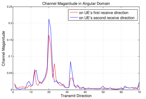
Figure 2: Illustration of angular domain channel with the ITU-R IMT-Advanced model in Urban Micro scenario [36]. The number of antennas at the BS and UE are 70 and 2, respectively. As can been seen, (i) the angular domain channel are sparse; (ii) the angular domain channel on different receive directions has simultaneous channel support.

Definition 4 (Massive MIMO Channel Model)

Let $\mathbf{h}_{j}\in\mathbb{C}^{N\times 1}$ be the $j$-th row vector of $\mathbf{H}_{a}\in\mathbb{C}^{N\times M}$. The channel matrix $\mathbf{H}_{a}$ satisfies: $\textrm{supp}(\mathbf{h}_{1})=\cdots\textrm{supp}(\mathbf{h}_{N})\triangleq\mathcal{T}$, where $\mathcal{T}$ is the channel support and $\left|\mathcal{T}\right|\leq\bar{s}$. Furthermore, the elements in $(\mathbf{H}_{a})_{\mathcal{T}}$ are i.i.d. complex Gaussian variables with zero mean and unit variance.

Note that $\bar{s}$ is a statistical upper bound on the number of spatial paths from the BS to the UE. In practice, the channel sparsity levels depend on the large scale properties of the scattering environment and changes slowly and hence information like $\bar{s}$ can be obtained at the UE from prior offline measurements. On the other hand, the channel paths are temporarily correlated so that consecutive frames would share some common channel paths. As a result, we can utilize the prior support information (Definition 2) in massive MIMO scenarios. Specifically, in the prior support information $(\mathcal{T}_{0},s_{c})$, $\mathcal{T}_{0}$ is the estimated channel support in the previous frame and $s_{c}$ characterizes the size of common channel paths between $\mathcal{T}_{0}$ and $\mathcal{T}$, i.e., $\left|\mathcal{T}_{0}\bigcap\mathcal{T}\right|\geq s_{c}$.

Remark 7 (Practical Considerations)

In practice, we usually need to estimate a sequence of channels $\mathbf{H}_{[1]}$, $\mathbf{H}_{[2]}$ … where $\mathbf{H}_{[i]}$ is the channel from the BS to the UE in the $i$-th frame [36]. At the very beginning, we don’t have prior channel estimations and hence we can set the prior channel support information $(\mathcal{T}_{0},s_{c})$ to be $\mathcal{T}_{0}=\emptyset$, $s_{c}=0$. At later stages when we have already obtained some prior channel estimations, the estimated channel support in the previous frame (e.g., $\mathbf{H}_{[i-1]}$) can act as the prior support $\mathcal{T}_{0}$ for the present time (e.g., $\mathbf{H}_{[i]}$). On the other hand, due to the slowly varying propagation environment between the BS and UE [13, 14] (as illustrated in Figure 3), it is likely that the size of the common support between consecutive channels, i.e., $\mathbf{H}_{[i-1]}$, $\mathbf{H}_{[i]}$, changes slowly so that we can gradually obtain a reliable statistical information as $s_{c}$. For instance, we can select $s_{c}$ to satisfy $\textrm{Pr}(\left|\mathcal{T}_{i-1}\bigcap\mathcal{T}_{i}\right|\geq s_{c})\geq 1-\epsilon$ for some small $\epsilon$, $0<\epsilon<1$ from prior channel measurements based on long term stochastic learning and estimation [37]. Note that a larger $s_{c}$ indicates a stronger temporal correlation between channels of consecutive frames. ∎

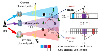
Figure 3: Illustration of point-to-point massive MIMO system in which the previous and current frames share some common spatial channel paths $\mathcal{T}_{0}\bigcap\mathcal{T}$ due to the slowly varying scattering environment. As such, the estimated channel support $\mathcal{T}_{0}$ in the previous frame can be utilized to enhance the CSIT estimation performance in the current frame.

VI-C Channel Recovery with the Proposed CS Framework

In this subsection, we talk about how to apply the proposed CS framework to conduct the recovery of $\mathbf{H}$ based on $\mathbf{Y}$.

Challenge 4: Apply the proposed framework of CS with prior support information in Section II, to conduct the recovery of $\mathbf{H}$ from (22).

First, equation (22) can be re-written as

$$\underset{\mathbf{Y}}{\underbrace{(\mathbf{\mathbf{Z}}^{H}\mathbf{U})}}=\underset{\Phi}{\underbrace{\sqrt{\frac{M}{T}}(\mathbf{V}\Theta)^{H}}}\underset{\mathbf{X}}{\underbrace{\sqrt{\frac{PT}{M}}(\mathbf{H}_{a})^{H}}}+\underset{\mathbf{N}}{\underbrace{\mathbf{W}^{H}\mathbf{U}}}.$$ (23)

Then (23) matches the CS measurement model in (3), where $(\mathbf{\mathbf{Z}}^{H}\mathbf{U})$ are measurements (role of $\mathbf{Y}$ in (3)), $\sqrt{\frac{M}{T}}(\mathbf{V}\Theta)^{H}$ is the measurement matrix ($\Phi$ in (3)), $\mathbf{W}^{H}\mathbf{U}$ is the noise ($\mathbf{N}$ in (3)) and $\sqrt{\frac{PT}{M}}(\mathbf{H}_{a})^{H}$ is the unknown signal source ($\mathbf{X}$ in (3)). Furthermore, $\sqrt{\frac{PT}{M}}(\mathbf{H}_{a})^{H}$ satisfies the general sparsity model in Section II-B with chunk size $1\times N$ ($d=1$, $L=N$ as in Definition 1). As such, the channel recovery problem is transformed the CS problem we consider in Section II.

Second, based on the transformed CS equation (23), we apply the proposed M-SP (Algorithm 1) to conduct the channel recovery by replacing the input parameter $\mathbf{Y}$ with $(\mathbf{\mathbf{Z}}^{H}\mathbf{U})$, $\Phi$ with $(\mathbf{V}\Theta)^{H}$, with $d$ set to be $d=1$. Denote the obtained algorithm output as $\hat{\mathbf{X}}$. Then the recovered channel $\hat{\mathbf{H}}$ for $\mathbf{H}$ is given by

$$\hat{\mathbf{H}}=\sqrt{\frac{M}{PT}}\mathbf{U}(\hat{\mathbf{X}})^{H}\mathbf{V}^{H}.$$ (24)

Third, we deploy the analytical results in Section IV to derive some performance results for $\hat{\mathbf{H}}$. Note that when $d=1$, the block-RIP is reduced to the conventional RIP [2]. Suppose that the pilot matrix $\sqrt{\frac{M}{T}}\Theta^{H}$ satisfies the RIP property and denote the corresponding $k$-th order RIP constants as $\delta_{k}$ (note that $\delta_{k}=\delta_{k|1}$ as $d=1$). Based on Theorem 1 and from the unitary invariance property of Frobenius norm, we obtain the following distortion bound.

Theorem 5 (Channel Recovery Performance)

If the $s_{2}$-th order RIP constant of $\Phi=\sqrt{\frac{M}{T}}\Theta^{H}$ satisfies $\delta_{s_{2}}\leq 0.246$, where $s_{2}=3\bar{s}+\min\left(0,\,\left|\mathcal{T}_{0}\right|-3s_{c}\right)$, then the average channel recovery distortion, i.e., $\mathbb{E}\left(\left\|\hat{\mathbf{H}}-\mathbf{H}\right\|_{F}\right)$ satisfies

$$\mathbb{E}\left(\left\|\hat{\mathbf{H}}-\mathbf{H}\right\|_{F}\right)$$

$$\leq \sqrt{\frac{M}{PT}}\left(\left(C_{4}+\frac{1}{\sqrt{1-\delta_{s_{2}}}}\right)\frac{\Gamma\left(NT+\frac{1}{2}\right)}{\Gamma(NT)}+\frac{\gamma}{\sqrt{1-\delta_{s_{2}}}}\right)$$ (25)

where $\gamma$ is threshold parameter in Algorithm 1, $\Gamma(\cdot)$ is the gamma function, $C_{4}$ is a constant given in Table III.

Proof:

From Theorem 1, equation (24), $\delta_{s_{2}}\leq 0.246$ and $s_{1}\leq s_{2}$, we derive $\left\|\hat{\mathbf{H}}-\mathbf{H}\right\|_{F}\leq\sqrt{\frac{M}{PT}}\left(C_{4}\eta+\frac{\gamma+\eta}{\sqrt{1-\delta_{s_{2}}}}\right)$. From this and $\mathbb{E}\left(\eta\right)=\mathbb{E}\left(\left\|\mathbf{W}\right\|_{F}\right)=\frac{\Gamma\left(NT+\frac{1}{2}\right)}{\Gamma(NT)}$, equation (25) is derived. ∎

From Theorem 5, as the transmit SNR $P\rightarrow\infty$, the average recovery distortion $\mathbb{E}\left(\left\|\hat{\mathbf{H}}-\mathbf{H}\right\|_{F}\right)\rightarrow 0$ and perfect channel recovery will be achieved. On the other hand, from the expression of $s_{2}\triangleq 3\bar{s}+\min\left(0,\,\left|\mathcal{T}_{0}\right|-3s_{c}\right)$, $s_{2}$ decreases as $s_{c}$ increases when $s_{c}\geq\frac{1}{3}\left|\mathcal{T}_{0}\right|$. In other words, a weaker RIP condition on the measurement matrix $\sqrt{\frac{M}{T}}\Theta^{H}$ is required as $s_{c}$ increases (e.g., we need $\delta_{3\bar{s}}\leq 0.246$ for $s_{c}=0$ and $\delta_{\bar{s}}\leq 0.246$ for $s_{c}=\left|\mathcal{T}_{0}\right|=\bar{s}$). This leads to a smaller requirement on the number of training pilot $T$ [2]. From this, we conclude that a larger strength of temporal correlation on the channel support (i.e., larger $s_{c}$) can enjoy a better reduction on the number of training pilots in massive MIMO systems. On the other hand, if we apply the conservative M-SP (Algorithm 2) instead of M-SP (Algorithm 1) to conduct the channel recovery, we can obtained a similar recovery performance result as in Theorem 5 by deploying Theorem 3 (details are omitted to avoid duplication).

VI-D Discussion on the Pilot Matrix $\Theta$

Note that we have not discussed the design of the pilot matrix $\Theta$ so that the aggregate measurement matrix $\Phi=\sqrt{\frac{M}{T}}\Theta^{H}$ in (23) can satisfy the RIP condition in Theorem 5. In the CS literature, matrices randomly generated from sub-Gaussian distribution [1] can satisfy the RIP with overwhelming probability and this randomized generation method has also been widely used. Following this convention, the elements of the pilot matrix $\Theta\in\mathbb{C}^{M\times T}$ can be generated from i.i.d. sub-Gaussian distribution (e.g., $\{\sqrt{\frac{1}{M}},-\sqrt{\frac{1}{M}}\}$ with equal probability). Using this method, from [2], when the length $T$ of the training pilot satisfies $T\geq c_{1}k\log M$, the probability that the CS measurement matrix $\Phi=\sqrt{\frac{M}{T}}\Theta^{H}$ in (23) satisfies a prescribed $k$-th order RIP condition $\delta_{k}\triangleq\delta$ will be no less than $1-\mathcal{O}\left(\textrm{exp}(-c_{2}T)\right)$, where $c_{1}$ and $c_{2}$ are some positive constants depending on $\delta$ [2].

VI-E Discussion of Other Possible Applications

In fact, the proposed framework can potentially be applied to many other areas, including wireless sensor networks (WSN) [38] and magnetic resonance imaging (MRI) [39] in which the target sparse signals usually demonstrate strong temporal correlations. To apply the proposed scheme, one can learn the statistical information $s_{c}$ (which characterizes the size of the shared common support between two consecutive signals) using the tools of stochastic learning and estimation [37]. In this work, we have proposed two algorithms, namely the M-SP and the conservative M-SP to conduct the signal recovery. For a specific application scenario, if the uncertainty on $s_{c}$ is small, then one should use the M-SP algorithm for better performance. On the other hand, if the underlying uncertainty on model parameter of $s_{c}$ is large, then one would prefer conservative M-SP for robustness. The robustness of conservative M-SP with respect to model mismatch on $s_{c}$ is illustrated in Figure 7 (will be elaborated in Section VII.D).

VII Numerical Results

In this Section, we consider the scenario of sparse channel estimation in massive MIMO systems as in Section VI to verify the effectiveness of the proposed framework. Specifically, we compare the performance of the proposed M-SP and conservative M-SP with the following baselines:

• Baseline 1 (SP): Deploy conventional SP [6] to recover the massive MIMO channel.

• Baseline 2 (Basis Pursuit): Deploy conventional basis pursuit [6] to recover the channel.

• Baseline 3 (modified Basis Pursuit): Deploy the modified basis pursuit proposed in [15] to recover the channel with blind exploitation of the prior support information.

• Baseline 4 (MMV-SP): Deploy an improved version of the SP [6] (corresponds the proposed M-SP with $s_{c}=0$) to adapt to the general sparsity model but without exploitation of the prior support information.

• Baseline 5 (AMP-MMV): Deploy the approximate message passing for multiple measurement vector problems (AMP-MMV) to conduct the channel recovery [9].

• Baseline 6 (Genie-aided LS): This serves as a performance upper bound scenario, in which the channel support $\mathcal{T}$ is assumed to be known and we directly use least square to recover the channel coefficients on $\mathcal{T}$.

We consider a narrow band (flat fading) point-to-point massive MIMO system with one BS and one UE, where the BS and UE have $M=200$ and $N=2$ antennas, respectively. Denote the average transmit SNR at the BS as $P$. We use the 3GPP spatial channel model (SCM) [36] to generate the channel coefficients and we consider that the UE has a rich local scattering environment as in [40]. Denote the channel to be estimated in the $i$-th frame as $\mathbf{H}_{i}$ and denote its corresponding channel support as $\mathcal{T}_{i}$. Suppose that the number of spatial paths from the BS broadside (corresponding to $|\mathcal{T}_{i}|$) are randomly generated as $|\mathcal{T}_{i}|\sim\mathcal{U}\left(\bar{s}-2,\bar{s}\right)$, $\forall i$, where $\mathcal{U}(a,b)$ denotes discrete uniform distribution over the set of integers $\{a,a+1,...,b\}$. Consider a slowly varying scattering scenario so that consecutive frames (i.e., $\mathcal{T}_{i}$, $\mathcal{T}_{i+1}$) share some spatial channel paths with size $|\mathcal{T}_{i}\bigcap\mathcal{T}_{i+1}|\sim\mathcal{U}\left(s_{c},s_{c}+2\right)$. The threshold parameter $\gamma$ in the proposed M-SP and conservative M-SP are given by $\gamma=\sqrt{2NT}$, where $T$ is the length of the training pilots. In baseline 2 [2] and baseline 3 [15], the threshold parameters in the constraint of the $l_{1}$-norm minimization are also set to be $\sqrt{2NT}$. In the following, we compare the normalized mean squared error (NMSE) [41] of the estimated channel with $G=1000$ channel realizations.

VII-A Channel Estimation Performance Versus Overhead $T$

In Figure 4, we compare the normalized mean squared error (NMSE) [41] of the estimated channel versus the length of the training pilot $T$, under transmit SNR $P=25$ dB, channel sparsity parameter $\bar{s}=18$, and prior channel quality parameter $s_{c}=10$. From this figure, we observe that the channel estimation performance increases as $T$ increases, and the proposed M-SP algorithm achieves a substantial performance gain over the Baseline 1-4. This is because the proposed M-SP adaptively exploits the prior channel support based on its quality parameter $s_{c}$ and it also adapts to the joint channel sparsity structure as illustrated in Section VI. Specifically, the performance gain of the M-SP over MMV-SP demonstrates the advantage of adaptively exploiting the prior channel support, and the performance gain of MMV-SP over SP indicates the benefits of adapting to the joint sparsity structures. On the other hand, note that the proposed conservative MSP has a smaller performance gain compared with the proposed M-SP. This is because the conservative M-SP utilizes the prior channel support in a more conservative manner and hence achieves less exploitation gain.

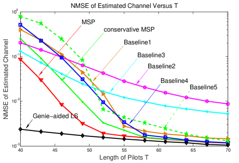
Figure 4: NMSE of estimated channel versus the pilot training length $T$ under $\bar{s}=18$, $s_{c}=10$ and transmit SNR $P=25$ dB.

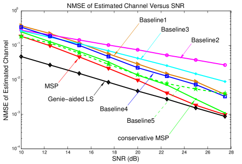
Figure 5: NMSE of estimated channel versus transmit SNR under $T=52$ and $\bar{s}=18$, $s_{c}=10$.

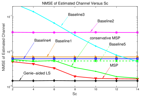
Figure 6: NMSE of estimated channel versus prior channel support quality parameter $s_{c}$ under transmit SNR $P=$25 dB, $T=52$ and $\bar{s}=18$.

VII-B Channel Estimation Performance Versus Transmit SNR $P$

In Figure 5, we compare the NMSE of the estimated channel versus the transmit SNR $P$ under $T=52$, $\bar{s}=18$ and $s_{c}=10$. From this figure, we observe that the proposed M-SP algorithm has substantial performance gain over the baselines and relatively a larger performance gain is achieved in higher SNR regions.

VII-C Channel Estimation Performance Versus Temporal Correlation Strength $s_{c}$

In Figure 6, we compare the NMSE of the estimated channel versus the prior support quality parameter $s_{c}$ (which indicates the strength of temporal correlation between channels of consecutive frames) under $T=52$, $\bar{s}=18$ and $P=25$ dB. From this figure, we observe that the channel estimation performance of the proposed M-SP and conservative M-SP gets better $s_{c}$ increases. This is because a larger $s_{c}$ means that a larger part of the prior channel support can be exploited. This simulation result also verifies the analysis in Section IV.

VII-D Channel Estimation Performance under Model mismatch

In this Section, we simulate the cases of model mismatch with incorrect information of $s_{c}$, i.e., $\left|\mathcal{T}_{0}\bigcap\mathcal{T}\right|<s_{c}$. Suppose that the size of shared channel support between consecutive frames is fixed to be $|\mathcal{T}_{i}\bigcap\mathcal{T}_{i+1}|=9$, $\forall i$, while the believed quality parameter $s_{c}$ varies from 8 to 13 (so that the believed prior support quality is incorrect when $s_{c}\in\{10,..,13\}$). Figure 7 illustrates the NMSE of the estimated channel versus believed quality parameter $s_{c}$ under transmit SNR $P=25$ dB and $\bar{s}=18$. From these figures, we observe that the performance of the M-SP degrades severely and a larger performance degradation is observed with a larger $s_{c}$ when $s_{c}\geq 10$ (i.e., a larger model mismatch). However, the conservative M-SP is stable and still enjoys performance gains over the baselines. These results demonstrate the robustness of the proposed conservative M-SP algorithm with model mismatches.

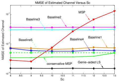
Figure 7: NMSE of estimated channel versus the believed $s_{c}$ under model mismatch with fixed $|\mathcal{T}_{i}\bigcap\mathcal{T}_{i+1}|=9$, $\forall i$. The other parameters are given by: transmit SNR $P=$25 dB, $T=52$ and $\bar{s}=18$.

VIII Conclusions and Future Works

In this paper, we consider CS problems with a prior support and the associated quality information available. Modified subspace pursuit recovery algorithms are designed to adaptively exploit the prior support information to enhance the signal recovery performance. By deploying the tools of block-RIP, we bound the recovery distortion and we show that the proposed algorithm converges with $\mathcal{O}\left(\log\mbox{SNR}\right)$ iterations. To tolerate possible model mismatch, we have further proposed a conservative design to have more robustness in cases of incorrect prior support information. Finally, we apply the proposed framework to channel estimation in massive MIMO systems with temporal correlation, to further reduce the length of the channel training pilots.

-A Proof of Lemma 1

The first two items directly follow from Definition 3. The following proves the third statement. First, we obtain $\sigma_{\max}\left(\Phi_{[\mathcal{T}_{1}\bigcup\mathcal{T}_{2}]}^{H}\Phi_{[\mathcal{T}_{1}\bigcup\mathcal{T}_{2}]}-\mathbf{I}\right)\leq\delta_{k_{1}+k_{2}|d}$ from Definition 3. Second, $\Phi_{[\mathcal{T}_{1}]}^{H}\Phi_{[\mathcal{T}_{2}]}$ is a submatrix of matrix $\Phi_{[\mathcal{T}_{1}\bigcup\mathcal{T}_{2}]]}^{H}\Phi_{[\mathcal{T}_{1}\bigcup\mathcal{T}_{2}]}-\mathbf{I}$. From the property that the spectral norm of a submatrix is always upper bounded by the spectral norm of the entire matrix, the third item is proved. The fourth inequality in Lemma 1 directly extends Lemma A.3 of [27].

-B Proof of Lemma 2

We first introduce the following equalities property:

$$(\mathbf{\Phi}^{H}\mathbf{R})^{[\mathcal{T}_{1}]}=\mathbf{\Phi}_{[\mathcal{T}_{1}]}^{H}\mathbf{R}$$ (26)

$$\mathbf{\Phi}_{[\mathcal{T}_{1}]}\mathbf{X}^{[\mathcal{T}_{1}]}=\mathbf{\Phi}_{[\mathcal{T}_{1}\backslash\mathcal{T}_{2}]}\mathbf{X}^{[\mathcal{T}_{1}\backslash\mathcal{T}_{2}]}+\mathbf{\Phi}_{[\mathcal{T}_{1}\bigcap\mathcal{T}_{2}]}\mathbf{X}^{[\mathcal{T}_{1}\bigcap\mathcal{T}_{2}]}$$ (27)

$$\mathbf{\Phi}_{[\mathcal{T}_{1}]}^{H}\left(\mathbf{I}-\mathbf{\Phi}_{[\mathcal{T}_{1}]}\mathbf{\Phi}_{[\mathcal{T}_{1}]}^{\dagger}\right) = \mathbf{0}$$ (28)

$$\left(\mathbf{I}-\mathbf{\Phi}_{[\mathcal{T}_{1}]}\mathbf{\Phi}_{[\mathcal{T}_{1}]}^{\dagger}\right)\mathbf{\Phi}_{[\mathcal{T}_{1}]} = \mathbf{0}$$

We first introduce the following inequalities property. Suppose $\sigma_{\min}\left(\mathbf{A}\right)$ and $\sigma_{\max}\left(\mathbf{A}\right)$ as the minimum and maximum singular values of $\mathbf{A}\in\mathbb{C}^{M\times S}$ ($M\geq S$), respectively, i.e., let $\mathbf{A}=U_{r}\varSigma U_{l}^{H}$, $\varSigma\in\mathbb{C}^{M\times S}$, be the singular decomposition of $\mathbf{A}$ , $\sigma_{\min}\left(\mathbf{A}\right)=\textrm{min}\left(\mbox{diag}\left(\varSigma\right)\right)$, $\sigma_{\max}\left(\mathbf{A}\right)=\max\left(\mbox{diag}\left(\varSigma\right)\right)$, we have

$$\sigma_{\max}\left(\mathbf{A}\mathbf{B}\right)\leq\sigma_{\max}\left(\mathbf{A}\right)\sigma_{\max}\left(\mathbf{B}\right).$$ (29)

$$\sigma_{\min}\left(\mathbf{A}\right)\left\|\mathbf{B}\right\|_{F}\leq\left\|\mathbf{A}\mathbf{B}\right\|_{F}\leq\sigma_{\max}\left(\mathbf{A}\right)\left\|\mathbf{B}\right\|_{F}.$$ (30)

Note that the above property (26)-(30) will be frequently used in the coming proof. Based on the selection criterion of $\mathcal{T}_{a}$, $\hat{\mathcal{T}}_{l}$, we obtain that (i) $\mathcal{T}_{a}\triangleq\left(\mathcal{T}_{b}\bigcup\mathcal{T}_{c}\right)\bigcup\hat{\mathcal{T}}_{l}$; (ii) $\left|\left(\mathcal{T}_{b}\bigcup\mathcal{T}_{c}\right)\right|\leq\bar{s}$, $\left|\hat{\mathcal{T}}_{l}\right|\leq\bar{s}$, $\left|\mathcal{T}\right|\leq\bar{s}$; (iii) Each of the three index set, i.e., $\left(\mathcal{T}_{b}\bigcup\mathcal{T}_{c}\right)$, $\hat{\mathcal{T}}_{l}$ and $\mathcal{T}$ contain at least $s_{c}$ elements from $\mathcal{T}_{0}$; Therefore,

$$\left|\mathcal{T}_{a}\right|\leq s_{1}\triangleq 2\bar{s}+\min\left(0,\,\left|\mathcal{T}_{0}\right|-2s_{c}\right).$$ (31)

$$|\mathcal{T}\bigcup\hat{\mathcal{T}}_{l}|\leq s_{1}\triangleq 2\bar{s}+\min\left(0,\,\left|\mathcal{T}_{0}\right|-2s_{c}\right).$$ (32)

$$|\mathcal{T}\bigcup\mathcal{T}_{a}|\leq s_{2}\triangleq 3\bar{s}+\min\left(0,\,\left|\mathcal{T}_{0}\right|-3s_{c}\right).$$ (33)

Based on (31)-(33), we obtain the following Lemma.

Lemma 3 (Iteration Property)

In the $l$-th iteration of Algorithm 1, the following three equations will be satisfied:

$$\left\|\mathbf{R}_{(l+1)}\right\|_{F} \leq\sqrt{1+\delta_{\bar{s}|d}}\left\|\mathbf{X}^{[\mathcal{T}\backslash\hat{\mathcal{T}}_{l+1}]}\right\|_{F}+\eta.$$ (34)

$$\left\|\mathbf{X}^{[\mathcal{T}\backslash\hat{\mathcal{T}}_{l+1}]}\right\|_{F} \leq\sqrt{1+\frac{4\delta_{s_{2}|d}^{2}\left(1+\delta_{s_{2}|d}\right)}{\left(1-\delta_{s_{1}|d}\right)}}\left\|\mathbf{X}^{[\mathcal{T}\backslash\mathcal{T}_{a}]}\right\|_{F}$$

$$+\frac{2}{\sqrt{1-\delta_{s_{1}|d}}}\eta.$$ (35)

$$\left\|\mathbf{X}^{[\mathcal{T}\backslash\mathcal{T}_{a}]}\right\|_{F} \leq\frac{2\delta_{s_{2}|d}}{\left(1-\delta_{\bar{s}|d}\right)\sqrt{1-\delta_{s_{1}|d}}}\left\|\mathbf{R}_{(l)}\right\|_{F}$$

$$+\left(\frac{2\delta_{s_{2}|d}}{\left(1-\delta_{\bar{s}|d}\right)\sqrt{1-\delta_{s_{1}|d}}}+\frac{2\sqrt{1+\delta_{\bar{s}|d}}}{1-\delta_{\bar{s}|d}}\right)\eta.$$ (36)

Proof:

The detailed proof for equations (34)-(36) are given in Appendix -C--E respectively. ∎

Combine equations (34)-(36), equation (12) in Lemma 2 is derived. Next, we prove equation (13) in Lemma 2. Based on (12), we obtain

$$\left\|\mathbf{R}_{(l)}\right\|_{F}\leq(C_{1})^{l}\left(\left\|\mathbf{R}_{(0)}\right\|_{F}-\frac{C_{2}\eta}{1-C_{1}}\right)+\frac{C_{2}\eta}{1-C_{1}}.$$ (37)

From $\left\|\mathbf{R}_{(0)}\right\|_{F}\leq\sqrt{1+\delta_{\bar{s}|d}}\left\|\mathbf{X}\right\|_{F}+\eta$ and the fact that

$$\left\|\mathbf{R}_{(l)}\right\|_{F} =\left\|\Phi(\mathbf{X}-\hat{\mathbf{X}}_{(l)})+\mathbf{N}\right\|_{F}$$

$$\geq\sqrt{1-\delta_{s_{1}|d}}\left\|\mathbf{X}-\hat{\mathbf{X}}_{(l)}\right\|_{F}-\eta,$$

equation (13) is derived.

-C Proof of equation (34)

From the expression of $\mathbf{R}_{(l+1)}$ in Step 2E of Algorithm 1, we obtain

$$\mathbf{R}_{(l+1)} =\left(\mathbf{I}-\Phi_{[\hat{\mathcal{T}}_{l+1}]}\Phi_{[\hat{\mathcal{T}}_{l+1}]}^{\dagger}\right)\left(\Phi_{[\mathcal{T}]}\mathbf{X}^{[\mathcal{T}]}+\mathbf{N}\right)$$

$$=\left(\mathbf{I}-\Phi_{[\hat{\mathcal{T}}_{l+1}]}\Phi_{[\hat{\mathcal{T}}_{l+1}]}^{\dagger}\right)\Phi_{[\mathcal{T}\backslash\hat{\mathcal{T}}_{l+1}]}\mathbf{X}^{[\mathcal{T}\backslash\hat{\mathcal{T}}_{l+1}]}$$

$$+\left(\mathbf{I}-\Phi_{[\hat{\mathcal{T}}_{l+1}]}\Phi_{[\hat{\mathcal{T}}_{l+1}]}^{\dagger}\right)\mathbf{N}$$ (38)

Note that $\mathbf{I}-\Phi_{[\hat{\mathcal{T}}_{l+1}]}\Phi_{[\hat{\mathcal{T}}_{l+1}]}^{\dagger}$ is a projection matrix hence $\sigma_{\max}\left(\mathbf{I}-\Phi_{[\hat{\mathcal{T}}_{l+1}]}\Phi_{[\hat{\mathcal{T}}_{l+1}]}^{\dagger}\right)\leq 1$. From (38), using properties in Lemma 1, equation (34) is proved.

-D Proof of equation (35)

From the selection criterion of Step 2.C in Algorithm 1, we obtain $\left\|\mathbf{Z}^{[\hat{\mathcal{T}}_{l+1}]}\right\|\geq\left\|\mathbf{Z}^{[\mathcal{T}]}\right\|$, which leads to

$$\left\|\mathbf{Z}^{[\mathcal{T}_{a}\backslash\mathcal{T}]}\right\|_{F}\geq\left\|\mathbf{Z}^{[\mathcal{T}_{a}\backslash\hat{\mathcal{T}}_{l+1}]}\right\|_{F}.$$ (39)

Denote $\mathbf{P}_{(\mathcal{T}_{a})}\triangleq\Phi_{[\mathcal{T}_{a}]}\left(\Phi_{[\mathcal{T}_{a}]}^{H}\Phi_{[\mathcal{T}_{a}]}\right)^{-1}\Phi_{[\mathcal{T}_{a}]}^{H}$. We further obtain

$$\mathbf{Z}^{[\mathcal{T}_{a}]}=\Phi_{[\mathcal{T}_{a}]}^{\dagger}\mathbf{Y}=\Phi_{[\mathcal{T}_{a}]}^{\dagger}\mathbf{P}_{(\mathcal{T}_{a})}\mathbf{Y}$$

$$= \Phi_{[\mathcal{T}_{a}]}^{\dagger}\mathbf{P}_{(\mathcal{T}_{a})}\left(\Phi_{[\mathcal{T}_{a}]}\mathbf{X}_{[\mathcal{T}_{a}]}+\Phi_{[\mathcal{T}\backslash\mathcal{T}_{a}]}\mathbf{X}_{[\mathcal{T}\backslash\mathcal{T}_{a}]}+\mathbf{N}\right)$$

$$\triangleq \mathbf{X}^{[\mathcal{T}_{a}]}+\mathbf{E}^{[\mathcal{T}_{a}]}+\Phi_{[\mathcal{T}_{a}]}^{\dagger}\mathbf{P}_{(\mathcal{T}_{a})}\mathbf{N}$$ (40)

where $\mathbf{E}\in\mathbb{C}^{N\times L}$ is given by $\mathbf{E}_{[\{1,...,K\}\backslash\mathcal{T}_{a}]}=\mathbf{0}$, $\mathbf{P}_{(\mathcal{T}_{a})}\Phi_{[\mathcal{T}\backslash\mathcal{T}_{a}]}\mathbf{X}_{[\mathcal{T}\backslash\mathcal{T}_{a}]}\triangleq\Phi_{[\mathcal{T}_{a}]}\mathbf{E}_{[\mathcal{T}_{a}]}$. From equation (40), we obtain

$$\left\|\mathbf{Z}^{[\mathcal{T}_{a}\backslash\mathcal{T}]}\right\|_{F}\leq\left\|\mathbf{E}^{[\mathcal{T}_{a}]}\right\|_{F}+\frac{1}{\sqrt{1-\delta_{s_{1}|d}}}\eta.$$ (41)

$$\left\|\mathbf{Z}^{[\mathcal{T}_{a}\backslash\hat{\mathcal{T}}_{l+1}]}\right\|_{F} \geq\sqrt{\left\|\mathbf{X}^{[\mathcal{T}\backslash\hat{\mathcal{T}}_{l+1}]}\right\|_{F}^{2}-\left\|\mathbf{X}^{[\mathcal{T}\backslash\mathcal{T}_{a}]}\right\|_{F}^{2}}$$

$$-\left\|\mathbf{E}^{[\mathcal{T}_{a}]}\right\|_{F}-\frac{1}{\sqrt{1-\delta_{s_{1}|d}}}\eta.$$ (42)

We further obtain

$$\sqrt{1-\delta_{s_{1}|d}}\left\|\mathbf{E}^{[\mathcal{T}_{a}]}\right\|_{F}\leq\left\|\Phi_{[\mathcal{T}_{a}]}\mathbf{E}^{[\mathcal{T}_{a}]}\right\|_{F}$$

$$= \left\|\mathbf{P}_{(\mathcal{T}_{a})}\Phi_{[\mathcal{T}\backslash\mathcal{T}_{a}]}\mathbf{X}^{[\mathcal{T}\backslash\mathcal{T}_{a}]}\right\|_{F}\overset{(a)}{\leq}\delta_{s_{2}|d}\sqrt{1+\delta_{s_{2}|d}}\left\|\mathbf{X}^{[\mathcal{T}\backslash\mathcal{T}_{a}]}\right\|_{F}$$ (43)

where $(a)$ comes from the fourth property in Lemma 1. Equation (43) leads to

$$\left\|\mathbf{E}^{[\mathcal{T}_{a}]}\right\|_{F}\leq\frac{\delta_{s_{2}|d}\sqrt{1+\delta_{s_{2}|d}}}{\sqrt{1-\delta_{s_{1}|d}}}\left\|\mathbf{X}^{[\mathcal{T}\backslash\mathcal{T}_{a}]}\right\|_{F}$$ (44)

Combining equation (39), (41), (42) and (44), we obtain equation (35).

-E Proof of equation (36)

At the beginning of the $l$-th iteration, the residue matrix $\mathbf{R}_{(l)}$ can be expressed as

$$\mathbf{R}_{(l)} =\left(\mathbf{I}-\Phi_{[\hat{\mathcal{T}}_{l}]}\Phi_{[\hat{\mathcal{T}}_{l}]}^{\dagger}\right)\left(\Phi_{[\mathcal{T}]}\mathbf{X}^{[\mathcal{T}]}+\mathbf{N}\right)$$

$$\triangleq\left[\begin{array}[t]{cc}\Phi_{[\mathcal{T}\backslash\hat{\mathcal{T}}_{l}]}&\Phi_{[\hat{\mathcal{T}}_{l}]}\end{array}\right]\tilde{\mathbf{X}}+\left(\mathbf{I}-\Phi_{[\hat{\mathcal{T}}_{l}]}\Phi_{[\hat{\mathcal{T}}_{l}]}^{\dagger}\right)\mathbf{N}$$ (46)

where $\tilde{\mathbf{X}}=\left[\begin{array}[t]{c}\begin{array}[]{c}\mathbf{X}^{[\mathcal{T}\backslash\hat{\mathcal{T}}_{l}]}\\ \mathbf{X}_{\triangle}\end{array}\end{array}\right]$ and $\mathbf{X}_{\triangle}=\mathbf{X}^{[\hat{\mathcal{T}}_{l}]}-\Phi_{[\hat{\mathcal{T}}_{l}]}^{\dagger}\Phi_{[\mathcal{T}]}\mathbf{X}^{[\mathcal{T}]}$. From the properties in Lemma 1, equation (46) and equation (32) we obtain

$$\left\|\mathbf{R}_{(l)}\right\|_{F}\geq\sqrt{1-\delta_{s_{1}|d}}\left\|\tilde{\mathbf{X}}\right\|_{F}-\eta$$ (47)

We further have the following equation

$$\left\|\mathbf{X}^{[\mathcal{T}\backslash\mathcal{T}_{a}]}\right\|_{F}\leq\frac{2\delta_{s_{2}|d}}{\left(1-\delta_{\bar{s}|d}\right)}\left\|\tilde{\mathbf{X}}\right\|_{F}+\frac{2\sqrt{1+\delta_{\bar{s}|d}}}{1-\delta_{\bar{s}|d}}\eta.$$ (48)

Note that equation (36) will be proved by combining equation (47) with (48). Therefore, we only need to prove (48) in the following. Since both $\left(\mathcal{T}_{c}\bigcup\mathcal{T}_{b}\right)$ and $\mathcal{T}$ contain $s_{c}$ chunks in $\mathcal{T}_{0}$, from the selection rule of Step 2. A, we have

$$\left\|\Phi_{[\mathcal{T}_{c}\bigcup\mathcal{T}_{b}]}^{H}\mathbf{R}_{(l)}\right\|_{F}\geq\left\|\Phi_{[\mathcal{T}]}^{H}\mathbf{R}_{(l)}\right\|_{F}$$ (49)

which derives $\left\|\Phi_{[(\mathcal{T}_{c}\bigcup\mathcal{T}_{b})\backslash\mathcal{T}]}^{H}\mathbf{R}_{(l)}\right\|_{F}\geq\left\|\Phi_{[\mathcal{T}\backslash(\mathcal{T}_{c}\bigcup\mathcal{T}_{b})]}^{H}\mathbf{R}_{(l)}\right\|_{F}$. From this and the fact that $\Phi_{[\hat{\mathcal{T}}_{l}]}^{H}\mathbf{R}_{(l)}=\mathbf{0}$, we further obtain

$$\left\|\Phi_{[(\mathcal{T}_{c}\bigcup\mathcal{T}_{b})\backslash(\mathcal{T}\bigcup\hat{\mathcal{T}}^{l})]}^{H}\mathbf{R}_{(l)}\right\|_{F}\geq\left\|\Phi_{[\mathcal{T}\backslash\mathcal{T}_{a}]}^{H}\mathbf{R}_{(l)}\right\|_{F}$$ (50)

The right hand side term in (50) is further bounded by

$$\left\|\Phi_{[(\mathcal{T}_{c}\bigcup\mathcal{T}_{b})\backslash(\mathcal{T}\bigcup\hat{\mathcal{T}}^{l})]}^{H}\mathbf{R}_{(l)}\right\|_{F}$$

$$= \left\|\Phi_{[(\mathcal{T}_{c}\bigcup\mathcal{T}_{b})\backslash(\mathcal{T}\bigcup\hat{\mathcal{T}}^{l})]}^{H}\times\vphantom{\left(\left[\begin{array}[t]{cc}\Phi_{[\mathcal{T}\backslash\hat{\mathcal{T}}^{l}]}&\Phi_{[\hat{\mathcal{T}}^{l}]}\end{array}\right]\tilde{\mathbf{X}}+\left(\mathbf{I}-\Phi_{[\hat{\mathcal{T}}^{l}]}\Phi_{[\hat{\mathcal{T}}^{l}]}^{\dagger}\right)\mathbf{N}\right)}\right.$$ (52)

$$\left.\left(\left[\begin{array}[t]{cc}\Phi_{[\mathcal{T}\backslash\hat{\mathcal{T}}_{l}]}&\Phi_{[\hat{\mathcal{T}}_{l}]}\end{array}\right]\tilde{\mathbf{X}}+\left(\mathbf{I}-\Phi_{[\hat{\mathcal{T}}_{l}]}\Phi_{[\hat{\mathcal{T}}_{l}]}^{\dagger}\right)\mathbf{N}\right)\right\|_{F}$$ (54)

$$\leq \delta_{s_{2}|d}\left\|\tilde{\mathbf{X}}\right\|_{F}+\sqrt{1+\delta_{\bar{s}|d}}\eta$$ (55)

The left hand side term in equation (50) is further bounded by

$$\left\|\Phi_{[\mathcal{T}\backslash\mathcal{T}_{a}]}^{H}\mathbf{R}_{(l)}\right\|_{F}$$

$$= \left\|\Phi_{[\mathcal{T}\backslash\mathcal{T}_{a}]}^{H}\times\vphantom{\left(\left[\begin{array}[t]{cc}\Phi_{[\mathcal{T}\backslash\hat{\mathcal{T}}^{l}]}&\Phi_{[\hat{\mathcal{T}}^{l}]}\end{array}\right]\tilde{\mathbf{X}}+\left(\mathbf{I}-\Phi_{[\hat{\mathcal{T}}^{l}]}\Phi_{[\hat{\mathcal{T}}^{l}]}^{\dagger}\right)\mathbf{N}\right)}\right.$$ (57)

$$= \left.\left(\left[\begin{array}[t]{cc}\Phi_{[\mathcal{T}\backslash\hat{\mathcal{T}}_{l}]}&\Phi_{[\hat{\mathcal{T}}_{l}]}\end{array}\right]\tilde{\mathbf{X}}+\left(\mathbf{I}-\Phi_{[\hat{\mathcal{T}}_{l}]}\Phi_{[\hat{\mathcal{T}}_{l}]}^{\dagger}\right)\mathbf{N}\right)\right\|_{F}$$ (59)

$$\geq \left\|\Phi_{[\mathcal{T}\backslash\mathcal{T}_{a}]}^{H}\left(\left[\begin{array}[t]{cc}\Phi_{[\mathcal{T}\backslash\mathcal{T}_{a}]}&\Phi_{[\mathcal{T}_{a}]}\end{array}\right]\right)\left[\begin{array}[t]{c}\begin{array}[]{c}\mathbf{X}^{[\mathcal{T}\backslash\mathcal{T}_{a}]}\\ \mathbf{X}_{\triangle}^{{}^{\prime}}\end{array}\end{array}\right]\right\|_{F}$$ (64)

$$-\sqrt{1+\delta_{\bar{s}|d}}\eta$$ (65)

where $\mathbf{X}_{\triangle}^{{}^{\prime}}$ is obtained by rewritten $\left[\begin{array}[t]{cc}\Phi_{[\mathcal{T}\backslash\hat{\mathcal{T}}_{l}]}&\Phi_{[\hat{\mathcal{T}}_{l}]}\end{array}\right]\tilde{\mathbf{X}}$ to be $\left(\left[\begin{array}[t]{cc}\Phi_{[\mathcal{T}\backslash\mathcal{T}_{a}]}&\Phi_{[\mathcal{T}_{a}]}\end{array}\right]\right)\left[\begin{array}[t]{c}\begin{array}[]{c}\mathbf{X}^{[\mathcal{T}\backslash\mathcal{T}_{a}]}\\ \mathbf{X}_{\triangle}^{{}^{\prime}}\end{array}\end{array}\right]$. Note that this $\mathbf{X}_{\triangle}^{{}^{\prime}}$ can always be found because $\hat{\mathcal{T}}_{l}\subseteq\mathcal{T}_{a}$. Furthermore $||\mathbf{X}_{\triangle}^{{}^{\prime}}||_{F}\leq\left\|\tilde{\mathbf{X}}\right\|_{F}$. Continuing the derivation in (65), we obtain

$$\left\|\Phi_{[\mathcal{T}\backslash\mathcal{T}_{a}]}^{H}\mathbf{R}_{(l)}\right\|_{F}$$

$$\geq \sigma_{\min}\left(\Phi_{[\mathcal{T}\backslash\mathcal{T}_{a}]}^{H}\Phi_{[\mathcal{T}\backslash\mathcal{T}_{a}]}\right)\left\|\mathbf{X}^{[\mathcal{T}\backslash\mathcal{T}_{a}]}\right\|_{F}$$

$$-\sigma_{\textrm{max}}\left(\Phi_{[\mathcal{T}\backslash\mathcal{T}_{a}]}^{H}\Phi_{[\mathcal{T}_{a}]}\right)\left\|\mathbf{X}_{\triangle}^{{}^{\prime}}\right\|_{F}-\sqrt{1+\delta_{\bar{s}|d}}\eta$$

$$\geq (1-\delta_{\bar{s}|d})\left\|\mathbf{X}^{[\mathcal{T}\backslash\mathcal{T}_{a}]}\right\|_{F}-\delta_{s_{2}|d}\left\|\tilde{\mathbf{X}}\right\|_{F}-\sqrt{1+\delta_{\bar{s}|d}}\eta.$$ (66)

Combine the results in equation (50), (55) and (66), we obtain

$$\delta_{s_{2}|d}\left\|\tilde{\mathbf{X}}\right\|_{F}+\sqrt{1+\delta_{\bar{s}|d}}\eta\geq$$

$$(1-\delta_{\bar{s}|d})\left\|\mathbf{X}^{[\mathcal{T}\backslash\mathcal{T}_{a}]}\right\|_{F}-\delta_{s_{2}|d}\left\|\tilde{\mathbf{X}}\right\|_{F}-\sqrt{1+\delta_{\bar{s}|d}}\eta$$

which further derives the desired equation (36).

-F Proof of Theorem 1

If Algorithm 1 stops from the condition of $\left\|\mathbf{R}_{(l+1)}\right\|_{F}\leq\gamma$, then the obtained solution $\mathbf{\hat{X}}=\hat{\mathbf{X}}_{(l+1)}$ and we obtain $\left\|\mathbf{X}-\hat{\mathbf{X}}\right\|_{F}\leq\frac{\gamma+\eta}{\sqrt{1-\delta_{s_{1}|d}}}$. If Algorithm 1 stops from the condition of $\left\|\mathbf{R}_{(l+1)}\right\|_{F}\geq\left\|\mathbf{R}_{(l)}\right\|_{F}$, then obtained solution $\mathbf{\hat{X}}=\hat{\mathbf{X}}_{(l)}$. From equation (12), we obtain

$$\left\|\mathbf{R}_{(l)}\right\|_{F}\leq\left\|\mathbf{R}_{(l+1)}\right\|_{F}\leq C_{1}\left\|\mathbf{R}_{(l)}\right\|_{F}+C_{2}\eta.$$

From $\delta_{s_{2}|d}<0.246$, we obtain $C_{1}<1$ and $\left\|\mathbf{R}_{(l)}\right\|_{F}\leq\frac{C_{2}\eta}{1-C_{1}}$. Further from $\mathbf{R}_{(l)}\geq\sqrt{1-\delta_{s_{1}|d}}\left\|\mathbf{X}-\hat{\mathbf{X}}\right\|_{F}-\eta$, we obtain $\left\|\mathbf{X}-\hat{\mathbf{X}}\right\|_{F}\leq C_{4}\eta$. Hence equation (14) is proved. Next, we prove (15). Note that when $\min_{k\in\mathcal{T}}\left\|\mathbf{X}[k]\right\|_{F}>\max\left(C_{4}\eta,\quad\frac{\gamma+\eta}{\sqrt{1-\delta_{s_{1}|d}}}\right)$, the identified signal support $\mathcal{\hat{T}}$ must be correct, i.e., $\mathcal{T}\subseteq\mathcal{\hat{T}}$. This can be proved via the contradiction method (i.e., $\exists i\in\mathcal{T}$, $i\notin\mathcal{\hat{T}}$. We obtain $\left\|\mathbf{X}-\hat{\mathbf{X}}\right\|_{F}\geq\left\|\mathbf{X}[i]\right\|_{F}>\max\left(C_{4}\eta,\quad\frac{\gamma+\eta}{\sqrt{1-\delta_{s_{1}|d}}}\right)$, which violates equation (14)). From $\mathcal{T}\subseteq\mathcal{\hat{T}}$, we obtain

$$\mathbf{X}-\hat{\mathbf{X}}=\mathbf{X}_{[\mathcal{\hat{T}}]}-\Phi_{[\mathcal{\hat{T}}]}^{\dagger}\left(\Phi_{[\mathcal{\hat{T}}]}^{\dagger}\mathbf{X}+\mathbf{N}\right)=-\Phi_{[\mathcal{\hat{T}}]}^{\dagger}\mathbf{N}$$

which further derives (15) from Lemma 1.

-G Proof of Theorem 2

First, $\left\|\mathbf{R}_{(0)}\right\|_{F}\leq\sqrt{1+\delta_{\bar{s}|d}}\rho^{\frac{1}{2}}+\eta$. Second, from (37), after $n$ iterations in Step 2 of Algorithm 1, the following inequality hold:

$$\left\|\mathbf{R}_{(n)}\right\|_{F} \leq\frac{C_{2}\eta}{1-C_{1}}+(C_{1})^{n}\left(\sqrt{1+\delta_{\bar{s}|d}}\rho^{\frac{1}{2}}+\eta-\frac{C_{2}\eta}{1-C_{1}}\right)$$ (67)

From (67), when $\gamma>\frac{C_{2}\eta}{1-C_{1}}$ , $n=n_{co}$, we must obtain $\left\|\mathbf{R}_{(n)}\right\|_{F}\leq\gamma$ and hence Step 2 of Algorithm 1 must have stopped after $n_{co}$ iterations, where $n_{co}$ is as given in Theorem 2).

-H Proof of Theorem 3

Note that for the conservative M-SP, we have (i) $\left|\mathcal{T}_{a}\right|\leq 2\bar{s}+s_{c}$, $\left|\mathcal{T}_{a}\bigcup\mathcal{T}\right|\leq s_{3}\triangleq 3\bar{s}+\min\left(s_{c},\left|\mathcal{T}_{0}\right|-\left|\mathcal{T}_{0}\bigcap\mathcal{T}\right|\right)$, $|\mathcal{T}\bigcup\hat{\mathcal{T}}_{l}|\leq 2\bar{s}$; (ii) equation (49), (39) for Step 2A and Step 2C, respectively, will hold no matter whether the quality information $s_{c}$ is correct or not. Following the proof of Appendix -B, we would obtain the following iteration property for the conservative M-SP,

$$\left\|\mathbf{R}_{(l+1)}\right\|_{F}\leq C_{5}\left\|\mathbf{R}_{(l)}\right\|_{F}+C_{6}\eta$$ (68)

where $C_{5}$, $C_{6}$ are modified correspondingly (compared with their counterpart $C_{1}$, $C_{2}$) and are given in Table IV. On the other hand, if Algorithm 1 stops from the condition of $\left\|\mathbf{R}_{(l+1)}\right\|_{F}\leq\gamma$, then the obtained solution $\mathbf{\hat{X}}=\hat{\mathbf{X}}_{(l+1)}$ satisfies $\left\|\mathbf{X}-\hat{\mathbf{X}}\right\|_{F}\leq\frac{\gamma+\eta}{\sqrt{1-\delta_{2\bar{s}|d}}}$ similar to Appendix -F. If Algorithm 1 stops from the condition of $\left\|\mathbf{R}_{(l+1)}\right\|_{F}\geq\left\|\mathbf{R}_{(l)}\right\|_{F}$, from (68), we obtain $\left\|\mathbf{R}_{(l)}\right\|_{F}\leq\frac{C_{6}\eta}{1-C_{5}}$. Furthermore, from $\mathbf{R}_{(l)}\geq\sqrt{1-\delta_{2\bar{s}|d}}\left\|\mathbf{X}-\hat{\mathbf{X}}\right\|_{F}-\eta$, we obtain $\left\|\mathbf{X}-\hat{\mathbf{X}}\right\|_{F}\leq C_{7}\eta$. Subsequently, equation (19) in Theorem 3 is proved. Based on (19), equation (20) can be obtained similar to (15).

References

- [1] S. Foucart and H. Rauhut, A mathematical introduction to compressive sensing. Springer, 2013.
- [2] E. Candes and T. Tao, “Decoding by linear programming,” IEEE Trans. Inf. Theory, vol. 51, no. 12, pp. 4203–4215, 2005.
- [3] J. A. Tropp and A. C. Gilbert, “Signal recovery from random measurements via orthogonal matching pursuit,” IEEE Trans. Inf. Theory, vol. 53, no. 12, pp. 4655–4666, 2007.
- [4] T. Blumensath and M. E. Davies, “Iterative hard thresholding for compressed sensing,” Applied and Computational Harmonic Analysis, vol. 27, no. 3, pp. 265–274, 2009.
- [5] D. Needell and J. A. Tropp, “CoSaMP: Iterative signal recovery from incomplete and inaccurate samples,” Applied and Computational Harmonic Analysis, vol. 26, no. 3, pp. 301–321, 2009.
- [6] W. Dai and O. Milenkovic, “Subspace pursuit for compressive sensing signal reconstruction,” IEEE Trans. Inf. Theory, vol. 55, no. 5, pp. 2230–2249, 2009.
- [7] J. Ziniel and P. Schniter, “Dynamic compressive sensing of time-varying signals via approximate message passing,” IEEE Trans. Signal Process., vol. 61, no. 21, pp. 5270–5284, 2013.
- [8] J. P. Vila and P. Schniter, “Expectation-maximization gaussian-mixture approximate message passing,” IEEE Trans. Signal Process., vol. 61, no. 19, pp. 4658–4672, 2013.
- [9] J. Ziniel and P. Schniter, “Efficient high-dimensional inference in the multiple measurement vector problem,” IEEE Trans. Signal Process., vol. 61, no. 2, pp. 340–354, 2013.
- [10] M. Wakin, J. Laska, M. Duarte, D. Baron, S. Sarvotham, D. Takhar, K. Kelly, and R. G. Baraniuk, “Compressive imaging for video representation and coding,” in Picture Coding Symposium, vol. 1, 2006.
- [11] M. P. Friedlander, H. Mansour, R. Saab, and Ö. Yilmaz, “Recovering compressively sampled signals using partial support information,” IEEE Trans. Inf. Theory, vol. 58, no. 2, pp. 1122–1134, 2012.
- [12] P. Ren, Y. Wang, Q. Du, and J. Xu, “A survey on dynamic spectrum access protocols for distributed cognitive wireless networks.” EURASIP J. Wireless Comm. and Networking, vol. 2012, p. 60, 2012.
- [13] K. Huang, R. W. Heath, and J. G. Andrews, “Limited feedback beamforming over temporally-correlated channels,” IEEE Trans. Signal Process., vol. 57, no. 5, pp. 1959–1975, 2009.
- [14] W. U. Bajwa, J. Haupt, A. M. Sayeed, and R. Nowak, “Compressed channel sensing: A new approach to estimating sparse multipath channels,” Proceedings of the IEEE, vol. 98, no. 6, pp. 1058–1076, 2010.
- [15] N. Vaswani and W. Lu, “Modified-CS: Modifying compressive sensing for problems with partially known support,” IEEE Trans. Signal Process., vol. 58, no. 9, pp. 4595–4607, 2010.
- [16] L. Jacques, “A short note on compressed sensing with partially known signal support,” Signal Processing, vol. 90, no. 12, pp. 3308–3312, 2010.
- [17] C. Herzet, C. Soussen, J. Idier, and R. Gribonval, “Exact recovery conditions for sparse representations with partial support information,” IEEE Trans. Inf. Theory, vol. 59, no. 11, pp. 7509–7524, Nov 2013.
- [18] R. Amel and A. Feuer, “Adaptive identification and recovery of jointly sparse vectors,” IEEE Trans. Signal Process., vol. 62, no. 2, pp. 354–362, Jan 2014.
- [19] Y. C. Eldar, P. Kuppinger, and H. Bolcskei, “Block-sparse signals: Uncertainty relations and efficient recovery,” IEEE Trans. Signal Process., vol. 58, no. 6, pp. 3042–3054, 2010.
- [20] Y. C. Eldar and M. Mishali, “Robust recovery of signals from a structured union of subspaces,” IEEE Trans. Inf. Theory, vol. 55, no. 11, pp. 5302–5316, 2009.
- [21] M. F. Duarte and Y. C. Eldar, “Structured compressed sensing: From theory to applications,” IEEE Trans. Signal Process., vol. 59, no. 9, pp. 4053–4085, 2011.
- [22] J. A. Tropp, A. C. Gilbert, and M. J. Strauss, “Algorithms for simultaneous sparse approximation. part I: Greedy pursuit,” Signal Processing, vol. 86, no. 3, pp. 572–588, 2006.
- [23] Y. C. Eldar and H. Rauhut, “Average case analysis of multichannel sparse recovery using convex relaxation,” IEEE Trans. Inf. Theory, vol. 56, no. 1, pp. 505–519, 2010.
- [24] Y. Barbotin, A. Hormati, S. Rangan, and M. Vetterli, “Estimation of sparse MIMO channels with common support,” IEEE Trans. Commun., vol. 60, no. 12, pp. 3705–3716, Dec. 2012.
- [25] C. Qiu, W. Lu, and N. Vaswani, “Real-time dynamic MR image reconstruction using kalman filtered compressed sensing,” in Proc. IEEE Int. Conf. Acoustics, Speech, Signal Processing (ICASSP). IEEE, 2009, pp. 393–396.
- [26] R. Giryes and M. Elad, “RIP-based near-oracle performance guarantees for SP, CoSaMP, and IHT,” IEEE Trans. Signal Process., vol. 60, no. 3, pp. 1465–1468, 2012.
- [27] L.-H. Chang and J.-Y. Wu, “An improved RIP-based performance guarantee for sparse signal recovery via orthogonal matching pursuit,” IEEE Trans. Inf. Theory, vol. 60, no. 9, pp. 5702–5715, Sept 2014.
- [28] E. G. Larsson, F. Tufvesson, O. Edfors, and T. L. Marzetta, “Massive MIMO for next generation wireless systems,” arXiv preprint arXiv:1304.6690, 2013. [Online]. Available: http://arxiv.org/abs/1304.6690
- [29] Y. Zhou, M. Herdin, A. M. Sayeed, and E. Bonek, “Experimental study of MIMO channel statistics and capacity via the virtual channel representation,” Univ. Wisconsin-Madison, Madison, Tech. Rep., Feb 2007.
- [30] P. Kyritsi, D. C. Cox, R. A. Valenzuela, and P. W. Wolniansky, “Correlation analysis based on MIMO channel measurements in an indoor environment,” IEEE J. Sel. Areas Commun., vol. 21, no. 5, pp. 713–720, 2003.
- [31] P.-H. Kuo, H. Kung, and P.-A. Ting, “Compressive sensing based channel feedback protocols for spatially-correlated massive antenna arrays,” in Proc. IEEE Wireless Commun. Networking Conf. (WCNC). IEEE, 2012, pp. 492–497.
- [32] X. Rao and V. Lau, “Distributed compressive CSIT estimation and feedback for FDD multi-user massive mimo systems,” IEEE Trans. Signal Process., vol. 62, no. 12, pp. 3261–3271, June 2014.
- [33] S. L. H. Nguyen and A. Ghrayeb, “Compressive sensing-based channel estimation for massive multiuser MIMO systems,” in Proc. IEEE Wireless Commun. Networking Conf. (WCNC). IEEE, 2013, pp. 2890–2895.
- [34] C.-K. Wen, S. Jin, K.-K. Wong, J.-C. Chen, and P. Ting, “Channel estimation for massive MIMO using gaussian-mixture bayesian learning,” IEEE Trans. Wireless Commun., vol. 14, no. 3, pp. 1356–1368, March 2015.
- [35] D. Tse and P. Viswanath, Fundamentals of wireless communication. Cambridge Univ Pr, 2005.
- [36] G. T. 25.996, “Universal mobile telecommunications system (UMTS); spacial channel model for multiple input multiple output (mimo) simulations,” 3GPP ETSI Release 9, Tech. Rep., 2010. [Online]. Available: http://www.3gpp.org/DynaReport/25996.htm
- [37] L. Bottou and N. Murata, “Stochastic approximations and efficient learning,” The Handbook of Brain Theory and Neural Networks, Second edition,. The MIT Press, Cambridge, MA, 2002.
- [38] R. Xie and X. Jia, “Transmission-efficient clustering method for wireless sensor networks using compressive sensing,” IEEE Trans. Parallel Distrib. Syst., vol. 25, no. 3, pp. 806–815, 2014.
- [39] S. Vasanawala, M. Alley, R. Barth, B. Hargreaves, J. Pauly, and M. Lustig, “Faster pediatric MRI via compressed sensing,” in Proc. Annual Meeting Soc. Pediatric Radiology (SPR), Carlsbad, CA, 2009.
- [40] M. Klessling, J. Speidel, and Y. Chen, “MIMO channel estimation in correlated fading environments,” in Proc. IEEE Vehicular Technology Conf. (VTC), vol. 2, 2003, pp. 1187–1191.
- [41] G. Sideratos and N. D. Hatziargyriou, “An advanced statistical method for wind power forecasting,” IEEE Trans. Power Systems, vol. 22, no. 1, pp. 258–265, 2007.